Reheating and dangerous relics
in pre-big bang string cosmology

Abstract

We discuss the mechanism of reheating in pre-big bang string cosmology and we calculate the amount of moduli and gravitinos produced gravitationally and in scattering processes of the thermal bath. We find that this abundance always exceeds the limits imposed by big-bang nucleosynthesis, and significant entropy production is required. The exact amount of entropy needed depends on the details of the high curvature phase between the dilaton-driven inflationary era and the radiation era. We show that the domination and decay of the zero-mode of a modulus field, which could well be the dilaton, or of axions, suffices to dilute moduli and gravitinos. In this context, baryogenesis can be accomodated in a simple way via the Affleck-Dine mechanism and in some cases the Affleck-Dine condensate could provide both the source of entropy and the baryon asymmetry.

UMN–TH–1906/00

TPI–MINN–00/26

GRP/00/541

hep-th/0006054

I Introduction

In the pre-big bang scenario (PBB) [1], the standard Friedman-Robertson-Walker (FRW) post-big bang picture emerges as the late-time history of a Universe which, in a prehistoric era (the so called pre-big bang era), underwent an inflationary expansion driven by the growth of the universal coupling of the theory. This latter phase is also referred to as dilaton driven inflation (DDI) as its super-inflationary dynamics are driven by the kinetic energy of the dilaton field. A crucial difference between the pre-big bang model and standard inflationary theories, is that in the PBB, the universe starts its evolution in a classical state, the most general perturbative solution of the tree-level low-energy string effective action. The analysis of this initial state, and its naturalness, has led to a debate, as to whether the initial conditions needed to solve the horizon and flatness problems can be deemed natural [2]. The problem of the graceful exit of the inflationary era is also an unsolved question. No-go theorems preventing the branch change from DDI to the dual solution of the FRW type have been demonstrated when either an axion field and a dilaton/axion potential or stringy fluid sources have been introduced in the tree-level effective action [3]. It is now recognized that if the branch change from DDI to FRW expansion is to occur, it should arise as a consequence of quantum loops effects and/or high curvature corrections, and encouraging progress has been made in this direction [4],[5]. Nevertheless, the PBB model remains an attractive variant to standard inflationary cosmology, notably since the initial state of the Universe lies in the weakly coupled regime of string theory, and its dynamics are thus well controled by the tree-level low-energy effective action. This is in contrast with standard inflationary theories which generically experience difficulties in extracting a well-suited Lagrangian for the inflaton field from a well-defined underlying fundamental theory, and in which the initial inflaton field values are usually of order the Planck scale.

In recent years, significant effort has been spent on understanding the physics of the pre-big bang initial state and its high curvature phase, and on extracting observational predictions for this scenario. In this respect, one should note the prediction of a stochastic background of gravitational waves [6], whose amplitude might be well above that predicted by models of standard inflation, as well as the amplification of quantum vacuum electromagnetic fluctuations  [7], due to the non-conformal coupling between the gravitational and the electromagnetic fields. More recently, it has been shown that the amplification of (universal) axion quantum fluctuations might provide adequate seeds for the formation of large-scale structures, and the resulting large and small angular scale anisotropies of the cosmic microwave background have been calculated [8, 9]. This provides a characteristic signal of non-Gaussian isocurvature perturbations. So far little attention has been paid to the phenomenology of the post-big bang FRW era, and notably on the mechanism of reheating. It has been proposed that reheating could proceed via gravitational particle production [11]. However, as we argue here, this predicts the presence of too many dangerous relics, much like non-oscillatory inflationary models [12], and notably an abundance of gravitationally interacting scalars (e.g. moduli) well in excess of the limits imposed by big bang nucleosynthesis (BBN) on the abundance of late decaying massive particles. On top of that one naively expects that in some PBB scenarios the FRW era starts at a high Hubble scale, of order the string scale $\sim 10^{17}\,{\rm GeV}$, and therefore gravitinos and moduli should also be produced copiously in scattering processes in the thermal bath.

These considerations warrant the present detailed study of the physics and phenomelogical problems of the PBB scenario in the post-pre-big bang era. We will find that indeed, for the variants of the PBB scenario hitherto proposed, there is inevitably need for significant entropy production. However, as we will argue, there exist various possible and natural sources of entropy production in pre-big bang models, notably the domination and decay of the zero-mode of a modulus, of the dilaton, or of axions, depending on the masses of these fields, which can dilute effectively moduli, gravitinos and monopoles. We will also show that this allows one to efficiently implement Affleck-Dine baryogenesis. In the following, we will thus focus on reheating, on the gravitino/moduli problem, and on the origin of the baryon asymmetry of the Universe. We will try to remain as general as possible, in particular with respect to the possible presence of an intermediate phase between DDI and FRW.

The outline of this paper is as follows. In Section II we review the dynamics of the PBB model, and some variants (as far as the intermediate phase is concerned) proposed in the literature. In Section III, we provide a book-keeping of the particle content of the Universe at the beginning of the FRW era, and explicitly show the need for entropy production. In Section IV we review the various possibilities for entropy production in the context of the PBB model when the transition from DDI to FRW occurs suddenly, and discuss baryogenesis. We defer the study of intermediate phases to Sections V and VI, since the consequences in that case are different but the logic of the argument is the same. We summarize our results in Section VII.

II The pre-big bang era

Let us first start by reviewing the different eras and dynamics envisaged in the PBB model. We shall restrict ourselves to the four-dimensional tree-level low-energy string effective action derived from heterotic string theory compactified on a six torus [13, 14], whose bosonic sector is described by: 

$$S_{\rm eff}=\frac{1}{2\lambda_{s}^{2}}\,\int d^{4}x\sqrt{-g}\,e^{-\varphi}\,\left[{\cal R}+g^{\mu\nu}\,\partial_{\mu}\varphi\,\partial_{\nu}\varphi-g^{\mu\nu}\,\partial_{\mu}\sigma_{a}\,\partial_{\nu}\sigma_{a}+{\cal L}_{\rm matter}\right]\,,$$ (1)

where $\lambda_{s}=\sqrt{\alpha^{\prime}}=\sqrt{8\pi}/M_{s}$ is the string-length parameter, $M_{s}$ denotes the string mass and the following relations hold:

$$\frac{e^{-\varphi}}{\lambda_{s}^{2}}=\frac{1}{l_{\rm pl}^{2}}=\frac{1}{8\pi\,G_{N}}\,,\quad\quad\alpha_{\rm GUT}(\lambda_{s}^{-1})=\frac{g^{2}}{4\pi}\,,\quad\quad g^{2}=e^{\varphi}\,.$$ (2)

Henceforth, we shall assume that at the present time $g_{0}\sim 0.01-0.1$. We restrict the internal compact space to a diagonal metric $g_{ab}=e^{2\sigma_{a}}\,\delta_{ab}$ with $a,b=4,\dots,9$, and we denote by $\varphi$ the effective four-dimensional dilaton field $\varphi=\phi_{10}-\sum_{a}\sigma_{a}$. The matter Lagrangian, ${\cal L}_{\rm matter}$, is composed of scalars, gauge fields and axions. We assume that the gauge and axion fields do not contribute to the cosmological background, i.e. we deal only with their quantum vacuum fluctuations. For the gauge fields, we consider the heterotic gauge field $A_{\mu}$ and the Kaluza-Klein gauge fields related to internal components of the metric and the three-form $H_{\mu\nu\rho}$, respectively $V_{\mu}^{\,\,a}$ and $W_{\mu}^{\,\,a}$ [13, 14]:

$${\cal L}_{\rm gauge\,fields}=\frac{1}{4}\,\alpha^{\prime}\,F_{\mu\nu}\,F^{\mu\nu}-\frac{1}{4}\,\alpha^{\prime}\,e^{2\sigma_{a}}\,V_{\mu\nu}^{\,\,\,\,a}\,V^{\mu\nu a}-\frac{1}{4}\,\alpha^{\prime}\,e^{-2\sigma_{a}}\,W_{\mu\nu a}\,W^{\mu\nu}_{\,\,\,\,\,a}\,,$$ (3)

where

$$F_{\mu\nu}=\partial_{\mu}A_{\nu}-\partial_{\nu}A_{\mu}\,,\quad\quad V_{\mu\nu}^{\,\,\,\,a}=\partial_{\mu}V_{\nu}^{\,\,a}-\partial_{\nu}V_{\mu}^{\,\,a}\,,\quad\quad W_{\mu\nu a}=\partial_{\mu}W_{\nu a}-\partial_{\nu}W_{\mu a}\,.$$ (4)

Finally, for the axion fields we have

$${\cal L}_{\rm axions}=-\frac{1}{2}\,e^{2\varphi}\,g^{\mu\nu}\,\partial_{\mu}A\,\partial_{\nu}A-\frac{1}{4}\,g^{\mu\nu}\,e^{-2\sigma_{b}}\,e^{-2\sigma_{c}}\,\partial_{\mu}B_{bc}\,\partial_{\nu}B_{bc}\,,$$ (5)

where $B_{ab}$ is the pseudo-scalar field associated to the compactified components of the anti-symmetric field living in ten dimensions, while $A$ is the axion related to the anti-symmetric tensor $H^{\mu\nu\rho}$ in four dimensions by the usual relation $H^{\mu\nu\rho}\equiv\epsilon^{\mu\nu\rho\sigma}\,e^{\varphi}\,\partial_{\sigma}A$ (where $\epsilon^{\mu\nu\rho\sigma}$ is the covariant full antisymmetric Levi-Civita tensor).

Let us consider first the simplest scenario in which the universe undergoes a super-inflationary evolution up to conformal time $\eta_{1}$, at Hubble scale $H_{1}\sim M_{s}$ and where the radiation dominated era is supposed to start, i.e. where the branch change from DDI to FRW occurs. The cosmological background during such DDI era is given, in conformal time, by

$$a(\eta)\sim(-\eta)^{\delta/(1-\delta)}\,,\quad\quad\varphi\sim\varphi_{1}+\frac{3\delta-1}{1-\delta}\,\log(-\eta)\,,$$ (6)

$$\sigma_{a}\sim\sigma_{a1}+\frac{\beta_{a}}{1-\delta}\,\log(-\eta)\,,\quad\quad\delta<0\,,\quad\quad\beta_{a}>0\,,$$ (7)

(note that with respect to the cosmological time $a(t)\sim(-t)^{\delta}$). A scalar field $\chi$ with canonical kinetic term evolves classically during DDI as:

$$\chi=\frac{1}{\sqrt{\alpha^{\prime}}}\,\frac{\beta_{\chi}}{1-\delta}\,\log(-\eta)\,,$$ (8)

where the parameters $\delta$, $\beta_{a}$, and $\beta_{\chi}$ satisfy the Kasner-type constraint:

$$1=3\,\delta^{2}+\sum_{a}\beta_{a}^{2}+\frac{1}{2}\,\beta_{\chi}^{2}\,.$$ (9)

This Kasner constraint can be rewritten as a relation between $\delta$ and an effective set of $\beta_{a}$ which parametrizes the evolution of other scalars, including internal moduli. We will thus neglect $\beta_{\chi}$ in the following. We have also assumed that the four-dimensional non-compact space-time expands isotropically, while the contraction of the six internal dimensions can be anisotropic. After the branch change has occurred, the metric is that of a spatially flat FRW space-time; at that point the kinetic energy of the dilaton has become negligible, and the dynamics are thus driven by radiation, so that $a(\eta>\eta_{1})\propto\eta$. The ulterior evolution of the dilaton is an unsolved question. We will assume that the dilaton is fixed in the radiation era [15], but we will also indicate explicitly the dependence on the string coupling $g_{1}$ (corresponding to the value of the coupling at the start of the radiation dominated phase) in our results. In particular, in the radiation era, the critical energy density $\rho_{c}$ as a function of the Hubble scale $H$ is: $\rho_{c}=(3/8\pi)g_{1}^{-2}H^{2}M_{s}^{2}$.

In some pre-big bang scenarios, the branch change from DDI to FRW is not instantaneous, and one considers an intermediate phase whose dynamics are obtained by taking into account higher order corrections to the low-energy effective action, such as finite size string effects and quantum string-loop effects. Unfortunately, a thorough knowledge of the dynamics and duration of this intermediate phase is still lacking. Cosmological solutions, which partially describe the high curvature phase, have nevertheless been proposed in the literature, most notably: (i) the “string” intermediate era, obtained by solving the equations of motion with only the first order corrections in $\alpha^{\prime}$ included [4], and (ii) the “dual-dilaton” intermediate phase [14] (see also [16] where this scenario was discussed in the more general framework of non-minimal models ), where one assumes that all $\alpha^{\prime}$ corrections are sufficient to provide by themselves (without including string-loop effects) a sudden branch-change from the DDI to another duality-related vacuum phase of the FRW type. In the “string” intermediate phase, the Hubble parameter is constant hence the dynamics is inflationary in the string frame, while in the “dual-dilaton” era, the Hubble parameter makes a bounce around its maximal value at the string mass. To simplify the discussion, we shall often assume in both cases that the internal dimensions have been stabilized in some way before the Universe enters the intermediate era. We fix at $\eta_{s}$ the time and $H_{s}$ the Hubble scale at which the Universe transits from the DDI era to the intermediate phase.

For the “string” intermediate phase, one obtains [4]:

$$a(\eta)\sim-\frac{1}{H_{s}\,\eta}\,,\quad\quad\varphi(\eta)\sim\varphi_{s}-2\zeta\,\log(-\eta)\,,\quad\quad\zeta\geq 0\,,$$ (10)

where $\zeta$ is an arbitrary parameter which governs the growing of the dilaton field, while with the “dual-dilaton” era [14]

$$a(\eta)\sim(-\eta)^{\theta/(1-\theta)}\,,\quad\quad\varphi\sim\varphi_{s}+\frac{3\theta-1}{1-\theta}\,\log(-\eta)\,,$$ (11)

and $\theta$ satisfies a Kasner constraint similar to Eq. (9).

III The post–pre-big bang era

In this section, we will consider the simplest version of the pre-big bang scenario with a sudden branch change from DDI to FRW, i.e. no intermediate phase of dynamics.

A Particle content due to gravitational production

The particles present at the very beginning of the radiation era result from gravitational particle production, in contrast to standard inflationary models, in which the post-inflationary era is dominated by inflaton condensates, which later decay into radiation in the reheating process. In fact, in the PBB scenario it is the kinetic energy of the dilaton, which drives the DDI phase, that is converted into gravitationally created particles, whose energy density will drive the FRW era. One can provide a simple estimate of the energy density contained in fields subject to gravitational particle creation, when no intermediate phase is present. If $a_{1}\equiv a(\eta_{1})$ is the scale factor at the branch change, then $\eta_{1}=(a_{1}H_{1})^{-1}$ (since $H\equiv a^{\prime}/a^{2}$), and $k_{1}=1/\eta_{1}$ represents a comoving wavenumber corresponding to the horizon size at the branch change. We also define $d\rho_{j}/d\ln k$ as the energy density spectrum in particle species $j$ as a function of wavenumber $k$. Then one obtains $d\rho_{j}/d\ln k\simeq 0$ for wavenumbers $k>k_{1}$, since those modes have remained within the horizon at all times, and could not be excited by the gravitational field. For fluctuations that exited the horizon during DDI and re-entered during FRW, i.e. those modes with wavenumber $k<k_{1}$, one generically obtains $d\rho_{j}/d\ln k\propto(k/k_{1})^{n_{j}^{\rm DDI}}$, and ${n_{j}^{\rm DDI}}$ is the spectral index acquired by species $j$ due to the dynamics of the DDI phase and transition into FRW. One imposes ${n_{j}^{\rm DDI}}>0$ so as to avoid infrared divergences, i.e. large-scale inhomogeneities (see also below) and the energy density in species $j$ is dominated by the energy density in the log interval around $k_{1}$, so that $\rho_{j}\sim(d\rho_{j}/d\ln k)_{|_{k_{1}}}$. Moreover, $k_{1}$ corresponds to the maximal amplified wavenumber: this mode has exited and re-entered the horizon at the same time, and roughly one particle has been produced in that mode. Gravitational particle production thus respects a democracy rule [11], namely all species share roughly the same energy density $\sim(a_{1}/a)^{4}H_{1}^{4}$, corresponding to one particle produced with momentum $H_{1}$ in phase space volume $\sim H_{1}^{3}$. Therefore, for all species $j$, $\rho_{j}\sim(a_{1}/a)^{4}H_{1}^{4}$ at times $\eta>\eta_{1}$, and consequently $\Omega_{j}\sim g_{1}^{2}(H_{1}/M_{s})^{2}$, where $\Omega_{j}$ denotes the density parameter in species $j$ and $g_{1}=e^{\varphi_{1}/2}$ is the value of the string coupling at the beginning of the radiation era [$M_{\rm Pl}(\eta_{1})=M_{s}/g_{1}$].

When more accurate calculations are performed, one finds that the above democracy rule is satisfied to within less than an order of magnitude between different species, and one obtains (with ${n_{j}^{\rm DDI}}\neq 0$)

$$\frac{d\rho_{j}}{d\log k}(\eta)\simeq\frac{{\cal N}_{j}}{2\pi^{2}}\,\left(\frac{a_{1}}{a}\right)^{4}H_{1}^{4}\,\left(\frac{k}{k_{1}}\right)^{n_{j}^{\rm DDI}}\quad\quad\eta>\eta_{1}\,,$$ (12)

and

$$\Omega_{j}(\eta)\simeq\frac{4\,{\cal N}_{j}}{3\pi}\,\left(\frac{H_{1}}{M_{s}}\right)^{2}\,g_{1}^{2}\,\left|1-\left(\frac{k_{\rm H}}{k_{1}}\right)^{n_{j}^{\rm DDI}}\right|\quad\quad\eta>\eta_{1}\,,$$ (13)

where ${\cal N}_{j}$ is the number of helicity states in species $j$. In Eq. (13), $k_{\rm H}$ is the wavenumber corresponding to the horizon size at time $\eta$, i.e. $k_{\rm H}\equiv 1/\eta$. In effect, only modes whose wavelength is smaller than the horizon size can be thought as propagating as particles, and can be included in the energy density. For modes whose wavelength is larger than the horizon size, the definition of an energy density becomes gauge-dependent. Nevertheless, since we impose $n_{j}^{\rm DDI}>0$ to avoid infra-red divergence problems, the contribution from the term in the absolute value in Eq. (13) is negligible for $\eta\gg\eta_{1}$, and the density parameter reduces to that deduced above by heuristic arguments, up to the fudge factor $4{\cal N}_{j}/3\pi$. At this point, one should note that some fields $j$, and notably the axion $A$, can actually have $n_{j}^{\rm DDI}<0$  (see Tab. I). Again, to avoid infra-red problems, we shall impose $n_{A}^{\rm DDI}>0$, that is $-1/3<\delta<0$ [19]. For the particular case of the PBB dynamics, it has been shown that the fields subject to particle production are those of spin 0, 1 and 2. One should mention that in Einstein gravity, abelian gauge fields are conformally invariant, and thus not gravitationally amplified; here, their conformal invariance is broken by the time evolution of the string coupling. Fermions (spin 1/2 and 3/2) are not produced [20] (see also Refs. [21, 22, 23, 24]), at least when effects of compactification are neglected (see below).

Particles	$n^{\rm DDI}$	$n$ (string phase)	$n$ (dual-dilaton phase)
moduli	$3$	$\left\{\begin{array}[]{ll}6-2\zeta&\zeta>\frac{3}{2}\\ 2\zeta&\zeta<\frac{3}{2}\end{array}\right.$	$4$
axion A	$-0.46\div 1$	$-2\zeta$	$-2.9\div-1.4$
axion $B_{ab}$	$-1\div 3$	$4-2\zeta$	$0\div 4$
Heterotic photons	$1\div 3$	$4-2\zeta$	$0.54\div 1.28$
KK photons	$1\div 3$	$4-2\zeta$	$-0.73\div 0.54$

TABLE I.: Spectral slopes for the particles which have been amplified gravitationally during the PBB phase assuming non-dynamical internal dimensions during the intermediate phases. The spectral indices in the three columns refer to fluctuations that exited the horizon during DDI, during the “string” phase, or re-entered during the “dual-dilaton” phase, respectively.

In Tab. I we summarize the values of the spectral slopes for all of the particles present in the model [14] assuming, for simplicity, non-dynamical internal dimensions during the intermediate phases. The range of values of $n^{\rm DDI}$ have been obtained varying $\delta$ and considering the possibility of having either one or six internal dynamical dimensions during DDI. Note that the spectral slope $n^{\rm DDI}$ for the moduli fields have been obtained while considering them as part of the background [19], while in the determination of $n$ with an intermediate phase, we neglect their presence in the background. Spectral slopes for other scalars depend in principle on their kinetic terms, and for simplicity we will assume that they have the same slopes as moduli fields, i.e. that they have canonical kinetic terms. The spectral slopes $n$ in the second and third columns correspond to the slopes for fluctuations that exited during the “string” phase and re-entered during FRW, or exited during DDI and re-entered during the “dual-dilaton” era, respectively, and will be discussed in Sections VI and V.

B Thermalization and reheating

In this section we analyse the thermalization and reheating process due to gravitational particle production. Let us start by considering the simple generic case with no intermediate phase. At Hubble scale $H_{1}$, all fields are produced with similar energy density (“democracy rule”). Let us denote by ${\cal N}_{r}$ the number of degrees of freedom in spin 0 and spin 1 fields charged under the gauge groups of the observable sector. Similarly, if ${\cal N}_{\rm tot}$ denotes the total number of degrees of freedom in spin 0, 1 and 2, i.e. that of the fields produced gravitationally, then the democracy rule implies that the fraction of energy density contained in radiation (in the observable sector) is $\Omega_{r}\simeq{\cal N}_{r}/{\cal N}_{\rm tot}$. If the number of particles charged under gauge group is much larger than the number of gauge singlets, we get $\Omega_{r}\sim 1$. However, in some string models, the number of gauge singlets may actually exceed the number of charged states, and in this case, one would generically expect $0.01\mathrel{\mathchoice{\lower 3.6pt\vbox{\halign{$\mathsurround=0pt\displaystyle\hfil#\hfil$\cr<\crcr\sim\crcr}}}{\lower 3.6pt\vbox{\halign{$\mathsurround=0pt\textstyle\hfil#\hfil$\cr<\crcr\sim\crcr}}}{\lower 3.6pt\vbox{\halign{$\mathsurround=0pt\scriptstyle\hfil#\hfil$\cr<\crcr\sim\crcr}}}{\lower 3.6pt\vbox{\halign{$\mathsurround=0pt\scriptscriptstyle\hfil#\hfil$\cr<\crcr\sim\crcr}}}}\Omega_{r}<1$. Henceforth, to keep the discussion generic we shall explicit the dependence on $\Omega_{r}$.

All fields carry typical energy $E\sim H_{1}(a_{1}/a)$, and the radiation number density $n_{r}\sim\Omega_{r}\rho_{c}/E$. Gauge non-singlets interact with cross-section $\sigma\sim\alpha^{2}/E^{2}$ and thus, thermalization occurs when the interaction rate $\Gamma_{r}\equiv n_{r}\sigma v\mathrel{\mathchoice{\lower 3.6pt\vbox{\halign{$\mathsurround=0pt\displaystyle\hfil#\hfil$\cr>\crcr\sim\crcr}}}{\lower 3.6pt\vbox{\halign{$\mathsurround=0pt\textstyle\hfil#\hfil$\cr>\crcr\sim\crcr}}}{\lower 3.6pt\vbox{\halign{$\mathsurround=0pt\scriptstyle\hfil#\hfil$\cr>\crcr\sim\crcr}}}{\lower 3.6pt\vbox{\halign{$\mathsurround=0pt\scriptscriptstyle\hfil#\hfil$\cr>\crcr\sim\crcr}}}}H$ ($v\sim 1$ is the relative velocity), i.e. at scale factor $a_{\rm th}$:

$$\frac{a_{\rm th}}{a_{1}}\simeq\,{\rm max}\left[1\,,\,8\Omega_{r}^{-1}g_{1}^{2}\alpha^{-2}\left(\frac{H_{1}}{M_{s}}\right)^{2}\right]\,.$$ (14)

For $\Omega_{r}\sim 1$, $g_{1}\sim 10^{-1}$, $\alpha=g_{1}^{2}/(4\pi)\sim 10^{-3}$ and $H_{1}\sim M_{s}$, thermalization occurs in $\simeq 9$ e-foldings of the scale factor at $H_{\rm th}\sim 10^{-8}\,H_{1}$. Let us observe that the value of $\alpha$ we have used differs from $\alpha_{\rm GUT}\sim 1/20$; this discrepancy, which is linked to the difference between the string scale $M_{s}$ and the GUT scale, is usually attributed to threshold effects. Note also that the various gauge fields $A_{\mu}$, $V_{\mu}^{a}$ and $W_{\mu}^{a}$ we introduced in the action, Eq. (3), can in principle have different gauge couplings depending on the compactification. For simplicity we assume a single coupling constant, $\alpha=g_{1}^{2}/4\pi$, which refers to the $A_{\mu}$ field.

Even before thermalization is achieved, one can define an effective entropy density $s=(4/3)\rho_{r}/T_{r}$, where $T_{r}=(30/\pi^{2})^{1/4}g_{\star}^{-1/4}\rho_{r}^{1/4}$ is an effective temperature, with $g_{\star}$ the number of degrees of freedom in the radiation after thermalization, i.e. including spin 1/2 fields that were not produced gravitationally but were re-created in scattering processes. This effective entropy will reduce to the standard entropy of the radiation once thermalization has been achieved, and $s\simeq 0.2g_{\star}^{1/4}\Omega_{r}^{3/4}(H_{1}M_{s}/g_{1})^{3/2}(a_{1}/a)^{3}$. Then, if $\Omega_{r}\simeq 1$, reheating is complete once radiation has thermalized. If $\Omega_{r}<1$, reheating would only be achieved once the fields that carry the remainder of the energy density have decayed to radiation. Such processes are constrained by big bang nucleosynthesis, which requires that at temperatures $T_{r}\mathrel{\mathchoice{\lower 3.6pt\vbox{\halign{$\mathsurround=0pt\displaystyle\hfil#\hfil$\cr<\crcr\sim\crcr}}}{\lower 3.6pt\vbox{\halign{$\mathsurround=0pt\textstyle\hfil#\hfil$\cr<\crcr\sim\crcr}}}{\lower 3.6pt\vbox{\halign{$\mathsurround=0pt\scriptstyle\hfil#\hfil$\cr<\crcr\sim\crcr}}}{\lower 3.6pt\vbox{\halign{$\mathsurround=0pt\scriptscriptstyle\hfil#\hfil$\cr<\crcr\sim\crcr}}}}1\,$MeV, $\Omega_{r}\simeq 1$ to within a few percent. Nevertheless, as we will argue in the following subsections, it will be necessary to release a vast amount of entropy to dilute the dangerous relics produced. This entropy production may be viewed as a period of secondary reheating.

C Dangerous relics

Using the above results, one can determine the number density of scalar fields with gravitational interactions present at the beginning of the radiation era and analyse their possible phenomenological consequences on BBN. In what follows, we will denote such scalar fields generically as moduli. Moduli are produced gravitationally as argued above, and one also expects them to be produced in scatterings of the thermal bath at time $\eta>\eta_{1}$. We will inspect each of these effects in turn, and discuss moduli and gravitinos.

1 Moduli

We adopt the generic notation $Y_{j}=n_{j}/s$ for the number-density $n_{j}$ to entropy-density $s$ ratio of species $j$; the entropy density in radiation can be written as before $s\simeq g_{\star}^{1/4}\rho_{r}^{3/4}$. Using Eq. (12) for $\rho_{r}$, one can rewrite $s\sim(2\pi^{2})^{-3/4}g_{\star}^{1/4}{\cal N}_{r}^{3/4}H_{1}^{3}(a_{1}/a)^{3}$. Note the dependence on ${\cal N}_{r}^{3/4}$ which counts the number of degrees of freedom produced gravitationally, namely those of spin 0 and 1. Due to supersymmetry, obviously ${\cal N}_{r}\sim g_{\star}/2$, since $g_{\star}$ accounts for these latter and their supersymmetric partners.

Similarly, the number density of moduli $n_{m}\simeq\rho_{m}/E_{m}$, with typical energy $E_{m}\simeq H_{1}(a_{1}/a)$, hence from Eq. (12) $n_{m}\simeq(1/2\pi^{2})H_{1}^{3}(a_{1}/a)^{3}$, and:

$$Y_{m}^{g}\simeq 0.3g_{\star}^{-1}\,,$$ (15)

where the superscript $g$ on $Y_{m}$ refers to gravitational production. For $g_{\star}\sim 10^{2}-10^{3}$, Eq. (15) gives $Y_{m}^{g}\sim 10^{-4}-10^{-3}$, which is well above the bounds imposed by BBN on the abundance of late decaying massive particles see e.g., [25]. Indeed, let us contrast these estimates with the upper limits on $Y_{m}$ imposed by big bang nucleosynthesis (BBN) from photon injection. When applied to the case of moduli and gravitinos whose lifetime $\sim\gamma^{-1}M_{\rm Pl}^{2}/m^{3}$, where $m\sim{\cal O}(100\,{\rm GeV})$ denotes the modulus/gravitino mass, and $\gamma$ is a fudge factor for the decay width ($\gamma\simeq 1/4$ in the case of the gravitino) these constraints become [26, 27]: $Y_{m}\mathrel{\mathchoice{\lower 3.6pt\vbox{\halign{$\mathsurround=0pt\displaystyle\hfil#\hfil$\cr<\crcr\sim\crcr}}}{\lower 3.6pt\vbox{\halign{$\mathsurround=0pt\textstyle\hfil#\hfil$\cr<\crcr\sim\crcr}}}{\lower 3.6pt\vbox{\halign{$\mathsurround=0pt\scriptstyle\hfil#\hfil$\cr<\crcr\sim\crcr}}}{\lower 3.6pt\vbox{\halign{$\mathsurround=0pt\scriptscriptstyle\hfil#\hfil$\cr<\crcr\sim\crcr}}}}10^{-15}$ for $m\simeq 100\,$GeV, $Y_{m}\mathrel{\mathchoice{\lower 3.6pt\vbox{\halign{$\mathsurround=0pt\displaystyle\hfil#\hfil$\cr<\crcr\sim\crcr}}}{\lower 3.6pt\vbox{\halign{$\mathsurround=0pt\textstyle\hfil#\hfil$\cr<\crcr\sim\crcr}}}{\lower 3.6pt\vbox{\halign{$\mathsurround=0pt\scriptstyle\hfil#\hfil$\cr<\crcr\sim\crcr}}}{\lower 3.6pt\vbox{\halign{$\mathsurround=0pt\scriptscriptstyle\hfil#\hfil$\cr<\crcr\sim\crcr}}}}10^{-14}$ for $m\simeq 300\,$GeV, and $Y_{m}\mathrel{\mathchoice{\lower 3.6pt\vbox{\halign{$\mathsurround=0pt\displaystyle\hfil#\hfil$\cr<\crcr\sim\crcr}}}{\lower 3.6pt\vbox{\halign{$\mathsurround=0pt\textstyle\hfil#\hfil$\cr<\crcr\sim\crcr}}}{\lower 3.6pt\vbox{\halign{$\mathsurround=0pt\scriptstyle\hfil#\hfil$\cr<\crcr\sim\crcr}}}{\lower 3.6pt\vbox{\halign{$\mathsurround=0pt\scriptscriptstyle\hfil#\hfil$\cr<\crcr\sim\crcr}}}}5\times 10^{-13}$ for $m\simeq 1\,$TeV . These bounds assume that the gravitino/modulus decays into photons with a branching ratio unity. Results weaker by $\sim 1-2$ orders of magnitude would be obtained if the modulus/gravitino decays only into neutrinos, since high energy neutrinos produce an electromagnetic shower by interacting with the cosmic neutrino background [28]. Moreover, stringent constraints in the high mass range $m\mathrel{\mathchoice{\lower 3.6pt\vbox{\halign{$\mathsurround=0pt\displaystyle\hfil#\hfil$\cr>\crcr\sim\crcr}}}{\lower 3.6pt\vbox{\halign{$\mathsurround=0pt\textstyle\hfil#\hfil$\cr>\crcr\sim\crcr}}}{\lower 3.6pt\vbox{\halign{$\mathsurround=0pt\scriptstyle\hfil#\hfil$\cr>\crcr\sim\crcr}}}{\lower 3.6pt\vbox{\halign{$\mathsurround=0pt\scriptscriptstyle\hfil#\hfil$\cr>\crcr\sim\crcr}}}}1\,$TeV would also be obtained if hadronic decay is allowed [29]. Thus a safe and generic limit is $Y_{m}\mathrel{\mathchoice{\lower 3.6pt\vbox{\halign{$\mathsurround=0pt\displaystyle\hfil#\hfil$\cr<\crcr\sim\crcr}}}{\lower 3.6pt\vbox{\halign{$\mathsurround=0pt\textstyle\hfil#\hfil$\cr<\crcr\sim\crcr}}}{\lower 3.6pt\vbox{\halign{$\mathsurround=0pt\scriptstyle\hfil#\hfil$\cr<\crcr\sim\crcr}}}{\lower 3.6pt\vbox{\halign{$\mathsurround=0pt\scriptscriptstyle\hfil#\hfil$\cr<\crcr\sim\crcr}}}}10^{-13}$, which corresponds to the celebrated limit on the reheating temperature $T_{\rm RH}\mathrel{\mathchoice{\lower 3.6pt\vbox{\halign{$\mathsurround=0pt\displaystyle\hfil#\hfil$\cr<\crcr\sim\crcr}}}{\lower 3.6pt\vbox{\halign{$\mathsurround=0pt\textstyle\hfil#\hfil$\cr<\crcr\sim\crcr}}}{\lower 3.6pt\vbox{\halign{$\mathsurround=0pt\scriptstyle\hfil#\hfil$\cr<\crcr\sim\crcr}}}{\lower 3.6pt\vbox{\halign{$\mathsurround=0pt\scriptscriptstyle\hfil#\hfil$\cr<\crcr\sim\crcr}}}}10^{9}\,$GeV in standard inflationary scenarios. When considering these limits and the above results for the PBB scenario, one realizes that entropy production to the level of at least $\sim 8-10$ orders of magnitude is required.

Moduli are also created in scattering processes of the thermal bath. The total amount of moduli present, at times $\eta\gg\eta_{1}$, can be obtained by solving the Boltzmann equation with adequate production and destruction terms, with $Y_{m}=Y^{g}_{m}$ as initial condition at $\eta=\eta_{1}$. This equation, when written as a function of radiation temperature $T$ reads:

$$\frac{dY^{s}_{m}}{dT}=-\left[\frac{1}{2}\,\sum_{a,b}\,Y_{a}\,Y_{b}\sigma_{a+b\to m+c}-\sum_{c}\,Y_{m}\,Y_{c}\,\sigma_{c+m\to a+b}\right]\,\frac{s}{HT}\,,$$ (16)

where the superscript $s$ on $Y_{m}$ refers to moduli produced by scattering processes. In the above equation, $Y_{a,b,c}$ denotes the number density to entropy density ratio of species $a,b,c$, and $\sigma_{a+b\to m+c}$ is the cross-section of the process $a+b\to m+c$. Generically, $a$ and $b$ are relativistic, in which case $Y_{a,b}\simeq 0.3/g_{\star}$ [note that the first sum in Eq. (16) is over degrees of freedom of $a$ and $b$]. Since we found previously $Y^{g}_{m}\sim 0.3/g_{\star}\sim Y_{a,b,c}$, which corresponds to equilibrium with radiation, the Boltzmann equation implies $dY_{m}^{s}/dT\sim 0$, i.e. the production/destruction of moduli in scattering processes is negligible as compared to $Y^{g}_{m}$, and the final $Y_{m}\sim Y^{g}_{m}$.

2 Gravitinos

It has been argued recently [20] that gravitinos should not be produced gravitationally in the PBB scenario, if the gravitino is effectively massless, i.e. if the superpotential $\langle W\rangle\sim 0$ in the DDI and FRW eras. During the DDI phase, one indeed expects $\langle W\rangle=0$ in a simple model. However, compactification of internal dimensions during DDI or non-perturbative effects to stabilize the dilaton in FRW should lead to the appearance of a superpotential, which would break the above condition, and result in gravitino production. Unfortunately, the magnitude of this mass term is very model-dependent and one cannot really determine the amount of gravitinos produced gravitationally. However, it should be noted that if one gravitino is produced per mode around the branch change frequency, corresponding to saturation of Fermi-Dirac statistics, one would find $Y^{g}_{3/2}\sim 0.3/g_{\star}$ per helicity state as in the case of moduli.

In any case, gravitinos are produced in scatterings of the thermal bath, in the same fashion as moduli and the Boltzmann equation (16) can be used substituting $m\to 3/2$ etc. If $Y^{g}_{3/2}\sim 0.3/g_{\star}$ per helicity state, corresponding to equilibrium, then as before $dY_{3/2}/dT\sim 0$. However if, as advocated in Ref. [18], gravitinos are not produced gravitationally in the PBB scenario, then $Y^{g}_{3/2}=0$, and an estimate of $Y_{3/2}$ is given by integrating the Boltzmann equation, neglecting annihilation and co-annihilation channels. This neglect is justified as long as the final value $Y_{3/2}\ll 1/g_{\star}$, i.e. as long as equilibrium is not reached. Thus one obtains, using the Boltzmann equation for gravitinos, the simple result [30, 31, 32]

$$Y_{3/2}^{s}\simeq{\Gamma\over H}\,Y_{a}$$ (17)

evaluated at the end of the PBB phase, where $\Gamma$ is the gravitino production rate and $Y_{a}$ denotes the number density to entropy density ratio in species a. For the particle content of the MSSM, the gravitino total production cross-section is $\Sigma_{\rm tot}\simeq 250\alpha/m_{\rm Pl}^{2}$ [33, 26] (see also [34] for finite-temperature contribution to the gravitino production cross-section), and therefore, integration of the Boltzmann equation (assuming radiation domination $a\propto\eta$) gives:

$$Y^{s}_{3/2}\simeq 100\alpha\,g_{\star}^{-7/4}\,g_{1}^{1/2}\,\Omega_{r}^{3/4}\,\left(\frac{H_{1}}{M_{s}}\right)^{1/2}.$$ (18)

For $g_{1}\sim 10^{-1}$, $\alpha=g_{1}^{2}/(4\pi)\sim 10^{-3}$, $\Omega_{r}\simeq 1$, $g_{\star}\sim 10^{2}-10^{3}$ and $H_{1}\sim M_{s}$, one thus finds $Y^{s}_{3/2}\sim 10^{-7}-10^{-5}$; this justifies our neglect of the annihilation channels in the Boltzmann equation. In any case, the destruction terms would ensure that $Y_{3/2}$ would never exceed its equilibrium value, so that $Y_{3/2}\sim{\rm min}\left[Y^{s}_{3/2}+Y^{g}_{3/2},1/g_{\star}\right]$ is a good approximation to the final abundance of gravitinos, independently of the value of $Y^{g}_{3/2}$.

It should be noted that Eq. (18) evaluates the number of gravitinos produced before radiation has thermalized [see Eq. (14)], at the Hubble scale $H_{1}$. Moreover, if fermions are not produced gravitationally, then the only charged non-singlets present at scale $H_{1}$ are those of spin 0 and 1, and the gravitino production cross-section should be smaller, since only channels $a+b\to\Psi_{3/2}+c$ involving $a,b$ of spin 0 or 1 should contribute. However, we do not expect this uncertainty to exceed an order of magnitude [30, 31, 32]. Furthermore, we used $\alpha\sim 10^{-3}$ as before, corresponding to $g_{1}\sim 0.1$, and we neglected the running of $\alpha$ between $M_{s}$ and $M_{\rm GUT}$. However, it is easy to check that calculating $Y_{3/2}$ with parameters corresponding to the GUT scale (Hubble scale $H_{\rm GUT}$, coupling $g_{1}$ and $\alpha_{\rm GUT}$), one would obtain the same result as above. This is because the higher cross-section at the GUT scale $\Sigma_{\rm tot}\propto\alpha_{\rm GUT}$, compensates for the smaller Hubble scale $H_{\rm GUT}$. Overall, we estimate the uncertainty in the calculation of $Y^{s}_{3/2}$ to be $\mathrel{\mathchoice{\lower 3.6pt\vbox{\halign{$\mathsurround=0pt\displaystyle\hfil#\hfil$\cr<\crcr\sim\crcr}}}{\lower 3.6pt\vbox{\halign{$\mathsurround=0pt\textstyle\hfil#\hfil$\cr<\crcr\sim\crcr}}}{\lower 3.6pt\vbox{\halign{$\mathsurround=0pt\scriptstyle\hfil#\hfil$\cr<\crcr\sim\crcr}}}{\lower 3.6pt\vbox{\halign{$\mathsurround=0pt\scriptscriptstyle\hfil#\hfil$\cr<\crcr\sim\crcr}}}}1$ order of magnitude, and the final $Y_{3/2}$ exceeds by far the bounds imposed by BBN, similarly to moduli.

3 Monopoles

Finally, it is important to mention that the PBB scenario also suffers from the usual monopole problem due to GUT symmetry breaking (see also Ref. [37]). Assuming that $p$ monopoles form per horizon volume $\sim(4\pi/3)H_{C}^{-3}$ at GUT symmetry breaking, one finds that the density parameter in monopoles today is

$$\Omega_{\rm M}h^{2}\sim 10^{11}\,p\,\left(\frac{m_{M}}{10^{16}\,{\rm GeV}}\right)\,\left(\frac{T_{C}}{10^{14}\,{\rm GeV}}\right)^{3}\,\Omega_{r}^{-1/2}\,,$$ (19)

where $T_{C}\sim 0.5\Omega_{r}^{1/4}H_{c}^{1/2}m_{\rm Pl}^{1/2}$ is the critical temperature of the phase transition, $m_{M}$ is the monopole mass, and $h$ denotes the Hubble constant today in units of 100km/s/Mpc. Naively, one expects $p\sim 1/8$ by counting the number of field orientations per horizon volume that would give rise to monopoles. However if the radius of nucleated bubbles at coalescence is much smaller than the horizon volume, one could actually obtain $p>1$ [38].

IV Entropy production and baryogenesis

The previous section indicated the need for a major source of entropy production in PBB models without an intermediate phase of dynamics. This is a stringent requirement, but, as we discuss below, sufficient entropy can be produced to solve the moduli/gravitino/monopole problems. Furthermore, as we argue in Section 4.B, this provides a natural framework for implementing baryogenesis in the PBB scenario.

A Sources of entropy and dilution of dangerous relics

The late decay of non-relativistic matter is a simple way to generate entropy. Consider in addition to the radiation background the presence of matter with an equation of state $p_{1}=w\rho_{1}$ and $w<1/3$. Let us denote the value of the scale factor at the time the energy density $\rho_{1}$ is equal to the radiation density, $\rho_{0}$, by $a_{\rm dom}$ corresponding to a Hubble scale $H_{\rm dom}$. For $a>a_{\rm dom}$, the Universe will be dominated by $\rho_{1}$ until its decay at $a_{\rm RH}$ corresponding to a Hubble scale $H_{\rm RH}$. To show the explicit dependence on the scale factor, let us write $\rho_{0}=g_{\star\rm dom}{\tilde{\rho}_{0}}/a^{4}$ where $g_{\star\rm dom}$ denotes the number of degrees of freedom at $a_{\rm dom}$ and $\rho_{1}={\tilde{\rho}_{1}}/a^{3(w+1)}$. Then at $a_{\rm dom}$ we have, $g_{\star\rm dom}{\tilde{\rho}_{0}}={\tilde{\rho}_{1}}a_{\rm dom}^{4-3(w+1)}$. Assuming instantaneous decay, we can denote the energy density of radiation produced in the decay by, $\rho_{2}=g_{\star\rm RH}{\tilde{\rho}_{2}}/a^{4}$ where $g_{\star\rm RH}$ denotes the number of degrees of freedom at reheating and $g_{\star\rm RH}{\tilde{\rho}_{2}}={\tilde{\rho}_{1}}a_{\rm RH}^{4-3(w+1)}$.

If we call $s_{0}$, the entropy density contained in $\rho_{0}$ at $a_{\rm RH}$, then $s_{0}={4\over 3}g_{\star\rm dom}{\tilde{\rho}_{0}}^{3/4}/a_{\rm RH}^{3}$. Similarly, the entropy in the radiation produced by the decay is $s_{1}={4\over 3}g_{\star\rm RH}{\tilde{\rho}_{2}}^{3/4}/a_{\rm RH}^{3}={4\over 3}g_{\star\rm RH}^{1/4}{\tilde{\rho}_{1}}^{3/4}a_{\rm RH}^{-9(w+1)/4}={4\over 3}g_{\star\rm RH}^{1/4}g_{\star\rm dom}^{3/4}{\tilde{\rho}_{0}}^{3/4}a_{\rm RH}^{-9(w+1)/4}/a_{\rm dom}^{[3-9(w+1)/4]}$. If we assume that the entropy release is large, we can write

$$\Delta s\equiv{s_{1}-s_{0}\over s_{0}}\simeq{s_{1}\over s_{0}}=\left({g_{\star\rm RH}\over g_{\star{\rm dom}}}\right)^{{1\over 4}}\left({a_{\rm RH}\over a_{\rm dom}}\right)^{[3-9(w+1)/4]}\Omega_{r}^{-3/4}$$ (20)

We can also express the entropy change in terms of the Hubble parameter using $(H_{\rm RH}/H_{\rm dom})^{2}=({a_{\rm dom}/a_{\rm RH}})^{3(w+1)}$ so that

$$\Delta s=\left(\frac{g_{\star\rm RH}}{g_{\star\rm dom}}\right)^{1/4}\,\left(\frac{H_{\rm dom}}{H_{\rm RH}}\right)^{[4-3(1+w)]/[2(1+w)]}\,\Omega_{r}^{-3/4}.$$ (21)

Note that we included explicitly in $s_{\rm dom}$ a factor of $\Omega_{r}^{3/4}$, which accounts for the fact that the FRW era may be driven by relativistic fields, but not by radiation (meaning gauge fields of the observable sector). We also assume that the dilaton is fixed to its present value, at the latest by the time of domination.

Depending on the equation of state, the exponent $[4-3(1+w)]/[2(1+w)]$ takes values from $1/2$ for $w=0$ (non-relativistic matter) to $\to+\infty$ for $w\to-1$ (cosmological constant), which is what effectively happens in standard inflation. Entropy can also be produced in first order phase transitions, albeit to a modest level, generally not more than $\sim 1$ order of magnitude [46].

In the following, we will be interested in the case of domination and decay of oscillations of a classical scalar field $\chi$ in its potential $V(\chi)$. In the present scenario we will assume that initially the field $\chi$ is displaced from its low-energy minimum by an amount $\chi_{0}\sim M_{\rm S}\sim m_{\rm Pl}$. This assumption is reasonable so long as the energy scales we are considering are much larger than the mass of the scalar field. If we stick with canonical kinetic terms for the moduli during the PBB phase and we appeal to no-scale supergravity models to describe the particle content at the beginning of the radiation era, the flat directions corresponding to the moduli are still preserved, at least at tree-level [47]. When supersymmetry breaking occurs the moduli will get a mass and we assume that the potential takes the simple form $V(\chi)\simeq m_{\chi}^{2}\,\chi^{2}/2$.

The dynamics of a scalar field in its potential in the expanding Universe are well-known: the field is overdamped, and remains frozen to its initial value $\chi_{0}$ as long as $H\mathrel{\mathchoice{\lower 3.6pt\vbox{\halign{$\mathsurround=0pt\displaystyle\hfil#\hfil$\cr>\crcr\sim\crcr}}}{\lower 3.6pt\vbox{\halign{$\mathsurround=0pt\textstyle\hfil#\hfil$\cr>\crcr\sim\crcr}}}{\lower 3.6pt\vbox{\halign{$\mathsurround=0pt\scriptstyle\hfil#\hfil$\cr>\crcr\sim\crcr}}}{\lower 3.6pt\vbox{\halign{$\mathsurround=0pt\scriptscriptstyle\hfil#\hfil$\cr>\crcr\sim\crcr}}}}m_{\chi}$. For $H\mathrel{\mathchoice{\lower 3.6pt\vbox{\halign{$\mathsurround=0pt\displaystyle\hfil#\hfil$\cr<\crcr\sim\crcr}}}{\lower 3.6pt\vbox{\halign{$\mathsurround=0pt\textstyle\hfil#\hfil$\cr<\crcr\sim\crcr}}}{\lower 3.6pt\vbox{\halign{$\mathsurround=0pt\scriptstyle\hfil#\hfil$\cr<\crcr\sim\crcr}}}{\lower 3.6pt\vbox{\halign{$\mathsurround=0pt\scriptscriptstyle\hfil#\hfil$\cr<\crcr\sim\crcr}}}}m_{\chi}$, the field oscillates with an amplitude $\propto a^{-3/2}$. Provided $\chi_{0}\mathrel{\mathchoice{\lower 3.6pt\vbox{\halign{$\mathsurround=0pt\displaystyle\hfil#\hfil$\cr<\crcr\sim\crcr}}}{\lower 3.6pt\vbox{\halign{$\mathsurround=0pt\textstyle\hfil#\hfil$\cr<\crcr\sim\crcr}}}{\lower 3.6pt\vbox{\halign{$\mathsurround=0pt\scriptstyle\hfil#\hfil$\cr<\crcr\sim\crcr}}}{\lower 3.6pt\vbox{\halign{$\mathsurround=0pt\scriptscriptstyle\hfil#\hfil$\cr<\crcr\sim\crcr}}}}m_{\rm Pl}$, the field comes to dominate the energy density after having started oscillating; if, as before, domination occurs at Hubble scale $H_{\rm dom}$, then for $H_{\rm dom}<H\mathrel{\mathchoice{\lower 3.6pt\vbox{\halign{$\mathsurround=0pt\displaystyle\hfil#\hfil$\cr<\crcr\sim\crcr}}}{\lower 3.6pt\vbox{\halign{$\mathsurround=0pt\textstyle\hfil#\hfil$\cr<\crcr\sim\crcr}}}{\lower 3.6pt\vbox{\halign{$\mathsurround=0pt\scriptstyle\hfil#\hfil$\cr<\crcr\sim\crcr}}}{\lower 3.6pt\vbox{\halign{$\mathsurround=0pt\scriptscriptstyle\hfil#\hfil$\cr<\crcr\sim\crcr}}}}m_{\chi}$, the amplitude of $\chi$ $\propto H^{3/4}$ since the Universe is still radiation dominated; for $H<H_{\rm dom}$, its amplitude $\propto H$. If we denote by $a_{\chi}$ the value of the scale factor when oscillations begin, then the oscillations dominate at $a_{\rm dom}=(m_{\rm Pl}/\chi_{0})^{2}a_{\chi}$. The field decays when $H\sim\Gamma_{\chi}$, where $\Gamma_{\chi}$ is the decay width of $\chi$; as before, we write $H_{\rm RH}=\Gamma_{\chi}$. Assuming that $\chi$ has gravitational interactions, $\Gamma_{\chi}\simeq\gamma_{\chi}m_{\chi}^{3}/M_{\rm Pl}^{2}$, where $\gamma_{\chi}$ is a fudge factor, we find that $\chi$’s decay at $a_{\rm RH}=\gamma_{\chi}^{-2/3}(\chi_{0}/m_{\rm Pl})^{2/3}(m_{\chi}/M_{\rm Pl})^{-4/3}a_{\chi}$. Inserting these expressions for $a_{\rm dom}$ and $a_{\rm RH}$ into Eq. (20) with $w=0$, we get

$$\Delta s\simeq 10^{12}\gamma_{\chi}^{-1/2}\left(\frac{m_{\chi}}{10^{6}\,{\rm GeV}}\right)^{-1}\left(\frac{\chi_{0}}{m_{\rm Pl}}\right)^{2}\Omega_{r}^{-3/4},$$ (22)

where we have set $g_{\star\rm dom}=200$, and $g_{\star\rm RH}=10$.

In the above, we chose to select a gravitational decay timescale for the $\chi$ field, as it represents the most efficient source of entropy, and $\chi$ is therefore the coherent mode of a hidden sector scalar or modulus. In principle it is possible to obtain more entropy production if $m_{\chi}\mathrel{\mathchoice{\lower 3.6pt\vbox{\halign{$\mathsurround=0pt\displaystyle\hfil#\hfil$\cr<\crcr\sim\crcr}}}{\lower 3.6pt\vbox{\halign{$\mathsurround=0pt\textstyle\hfil#\hfil$\cr<\crcr\sim\crcr}}}{\lower 3.6pt\vbox{\halign{$\mathsurround=0pt\scriptstyle\hfil#\hfil$\cr<\crcr\sim\crcr}}}{\lower 3.6pt\vbox{\halign{$\mathsurround=0pt\scriptscriptstyle\hfil#\hfil$\cr<\crcr\sim\crcr}}}}10^{6}\,$GeV. However the reheating temperature, given by

$$T_{\chi\rm RH}\simeq 0.6\,{\rm GeV}\,\gamma_{\chi}^{1/2}\,\left(\frac{g_{\star\rm RH}}{10}\right)^{-1/4}\,\left(\frac{m_{\chi}}{10^{6}\,{\rm GeV}}\right)^{3/2}\,,$$ (23)

should not be lower than $\simeq 10\,$MeV for BBN to proceed unaffected, which requires $m_{\chi}\mathrel{\mathchoice{\lower 3.6pt\vbox{\halign{$\mathsurround=0pt\displaystyle\hfil#\hfil$\cr>\crcr\sim\crcr}}}{\lower 3.6pt\vbox{\halign{$\mathsurround=0pt\textstyle\hfil#\hfil$\cr>\crcr\sim\crcr}}}{\lower 3.6pt\vbox{\halign{$\mathsurround=0pt\scriptstyle\hfil#\hfil$\cr>\crcr\sim\crcr}}}{\lower 3.6pt\vbox{\halign{$\mathsurround=0pt\scriptscriptstyle\hfil#\hfil$\cr>\crcr\sim\crcr}}}}6\times 10^{4}\,\gamma_{\chi}^{-1/3}$GeV [25]. Furthermore gravitinos are re-created in $\chi$ decay to the level of: $Y_{3/2}\simeq 10^{-13}(m_{3/2}/1\,{\rm TeV})^{2}(m_{\chi}/10^{6}\,{\rm GeV})^{-3/2}$, so that one should impose $m_{\chi}\mathrel{\mathchoice{\lower 3.6pt\vbox{\halign{$\mathsurround=0pt\displaystyle\hfil#\hfil$\cr>\crcr\sim\crcr}}}{\lower 3.6pt\vbox{\halign{$\mathsurround=0pt\textstyle\hfil#\hfil$\cr>\crcr\sim\crcr}}}{\lower 3.6pt\vbox{\halign{$\mathsurround=0pt\scriptstyle\hfil#\hfil$\cr>\crcr\sim\crcr}}}{\lower 3.6pt\vbox{\halign{$\mathsurround=0pt\scriptscriptstyle\hfil#\hfil$\cr>\crcr\sim\crcr}}}}10^{5}-10^{6}\,{\rm GeV}$ [35]. Finally, if $R-$parity holds, one needs to achieve $T_{\chi\rm RH}\mathrel{\mathchoice{\lower 3.6pt\vbox{\halign{$\mathsurround=0pt\displaystyle\hfil#\hfil$\cr>\crcr\sim\crcr}}}{\lower 3.6pt\vbox{\halign{$\mathsurround=0pt\textstyle\hfil#\hfil$\cr>\crcr\sim\crcr}}}{\lower 3.6pt\vbox{\halign{$\mathsurround=0pt\scriptstyle\hfil#\hfil$\cr>\crcr\sim\crcr}}}{\lower 3.6pt\vbox{\halign{$\mathsurround=0pt\scriptscriptstyle\hfil#\hfil$\cr>\crcr\sim\crcr}}}}1\,$GeV for annihilations of LSPs to take place efficiently enough to reduce its abundance to cosmologically acceptable levels [36]. Overall, it seems that $\Delta s\sim 10^{12}$ represents, within an order of magnitude, the largest entropy production that is compatible with cosmological bounds for a displaced oscillating modulus.

If at time $\eta_{1}$, $Y_{m}\sim 0.3g_{\star}^{-1}$, the final abundance of moduli is given by:

$$Y_{m}\sim 2\times 10^{-15}\gamma_{\chi}^{1/2}\left(\frac{m_{\chi}}{10^{6}\,{\rm GeV}}\right)\left(\frac{\chi_{0}}{m_{\rm Pl}}\right)^{-2}\Omega_{r}^{3/4}\,,$$ (24)

where we assumed, for simplicity, $g_{\star}\simeq 200$ for the number of degrees of freedom in the radiation bath at time $\eta_{1}$, and $\Omega_{r}$ represents as before the fraction of energy density stored in particles charged under gauge groups. For higher $g_{\star}$, the numerical prefactor is further reduced as $(g_{\star}/200)^{-1}$. We found in the previous section that the abundance of gravitinos produced gravitationally and in scattering processes does not exceed the abundance of moduli, and therefore the above estimate provides an upper limit to the final abundance of gravitinos. As for the monopole density parameter today, it is given by:

$$\Omega_{M}h^{2}\simeq 0.1p\,\gamma_{\chi}^{1/2}\,\left(\frac{m_{M}}{10^{16}\,{\rm GeV}}\right)\,\left(\frac{T_{C}}{10^{14}\,{\rm GeV}}\right)^{3}\,\left(\frac{m_{\chi}}{10^{6}\,{\rm GeV}}\right)\,\left(\frac{\chi_{0}}{m_{\rm Pl}}\right)^{-2}\,\Omega_{r}^{1/4}\,.$$ (25)

This result was already obtained in Ref. [37], which studied the dilution of the monopole abundance through moduli oscillations and decay.

Therefore, an initial value $\chi_{0}\sim m_{\rm Pl}$ appears sufficient to solve the moduli/gravitino problem of the PBB scenario, and marginally sufficient with regards to the monopole problem. If $\chi_{0}\sim 10^{17}\,$GeV, it is still possible to dilute the moduli and gravitinos down to acceptable levels $Y_{m}\sim 10^{-13}$, but not monopoles. It should be pointed out, however, that the number $p$ of monopoles produced per horizon volume is uncertain, and furthermore, that annihilations of monopoles with antimonopoles have been neglected in the above calculations. As a matter of fact, in various patterns of symmetry breaking, it appears that the monopoles are tied by cosmic strings, in which case annihilation of monopoles and antimonopoles would be highly efficient, leading to a scaling regime with one monopole per horizon volume at all times [38, 39]. In this latter case, there would be no monopole problem at all.

It should also be noted that we did not mention the possible moduli problem associated with the coherent mode of those moduli whose mass $\mathrel{\mathchoice{\lower 3.6pt\vbox{\halign{$\mathsurround=0pt\displaystyle\hfil#\hfil$\cr<\crcr\sim\crcr}}}{\lower 3.6pt\vbox{\halign{$\mathsurround=0pt\textstyle\hfil#\hfil$\cr<\crcr\sim\crcr}}}{\lower 3.6pt\vbox{\halign{$\mathsurround=0pt\scriptstyle\hfil#\hfil$\cr<\crcr\sim\crcr}}}{\lower 3.6pt\vbox{\halign{$\mathsurround=0pt\scriptscriptstyle\hfil#\hfil$\cr<\crcr\sim\crcr}}}}10\,$TeV, even though we considered entropy production due to one such coherent mode with mass $\sim 10^{6}\,$GeV. As is well-known, an initial displacement of order $m_{\rm Pl}$ from the low-energy minimum of these moduli potentials would lead to a cosmological catastrophe: a reheating temperature $\mathrel{\mathchoice{\lower 3.6pt\vbox{\halign{$\mathsurround=0pt\displaystyle\hfil#\hfil$\cr<\crcr\sim\crcr}}}{\lower 3.6pt\vbox{\halign{$\mathsurround=0pt\textstyle\hfil#\hfil$\cr<\crcr\sim\crcr}}}{\lower 3.6pt\vbox{\halign{$\mathsurround=0pt\scriptstyle\hfil#\hfil$\cr<\crcr\sim\crcr}}}{\lower 3.6pt\vbox{\halign{$\mathsurround=0pt\scriptscriptstyle\hfil#\hfil$\cr<\crcr\sim\crcr}}}}1\,$keV and an enormous post-BBN entropy production $\mathrel{\mathchoice{\lower 3.6pt\vbox{\halign{$\mathsurround=0pt\displaystyle\hfil#\hfil$\cr>\crcr\sim\crcr}}}{\lower 3.6pt\vbox{\halign{$\mathsurround=0pt\textstyle\hfil#\hfil$\cr>\crcr\sim\crcr}}}{\lower 3.6pt\vbox{\halign{$\mathsurround=0pt\scriptstyle\hfil#\hfil$\cr>\crcr\sim\crcr}}}{\lower 3.6pt\vbox{\halign{$\mathsurround=0pt\scriptscriptstyle\hfil#\hfil$\cr>\crcr\sim\crcr}}}}10^{16}$ [40]. Once the modulus starts oscillating, it behaves as a condensate of zero momentum particles with abundance $n_{m}/s\sim 10^{7}(m/100\,{\rm GeV})^{-1/2}(\chi_{0}/m_{\rm Pl})^{2}\Omega_{r}^{-3/4}$, where $m$, $\chi_{0}$, $\Omega_{r}$ and $s$ denote respectively the mass, initial vev and radiation fraction of energy density when the modulus starts its oscillations, and the entropy contained in radiation. Hence, the above source of entropy cannot reduce sufficiently the abundance of these moduli, unless $\chi_{0}\mathrel{\mathchoice{\lower 3.6pt\vbox{\halign{$\mathsurround=0pt\displaystyle\hfil#\hfil$\cr<\crcr\sim\crcr}}}{\lower 3.6pt\vbox{\halign{$\mathsurround=0pt\textstyle\hfil#\hfil$\cr<\crcr\sim\crcr}}}{\lower 3.6pt\vbox{\halign{$\mathsurround=0pt\scriptstyle\hfil#\hfil$\cr<\crcr\sim\crcr}}}{\lower 3.6pt\vbox{\halign{$\mathsurround=0pt\scriptscriptstyle\hfil#\hfil$\cr<\crcr\sim\crcr}}}}10^{-4}m_{\rm Pl}$. Unfortunately there is no well accepted reason why at high energy, i.e. after the branch change, these moduli should lie close to their low-energy minimum, and this problem affects all cosmological models, not only the PBB scenario. Nevertheless, if the string vacuum is a point of enhanced symmetry, one would indeed expect the moduli to lie close to their low-energy minima at high energy scales [41]. In this respect, there is an interesting difference between the PBB scenario and the standard inflationary models. In effect, in this latter class of models, even if the coherent mode is not displaced at the classical level, the generation of quantum fluctuations on large wavelengths will generate an effective zero-mode on the scale of the horizon at the end of inflation, displaced from its low-energy minimum: the so-called quantum version of the moduli problem  [43, 22]. In the PBB scenario, since the spectrum of the fluctuations of a scalar field is very steep at very large wavelengths (spectral slope $=3$), its amplitude is small enough not to regenerate, at a quantum level, the zero-mode moduli problem.

Enhanced symmetry on the ground state manifold would not apply to the dilaton [41], and in this respect one could wonder whether the dilaton could not play the role of the $\chi$ field above, while other moduli would be fixed to their low-energy minimum for the above reason. Since the dilaton drives the DDI phase with its kinetic energy, and since it is not expected to lie exactly at the minimum of its low-energy potential at the end of DDI, this possibility seems rather natural in the framework of the PBB scenario. Furthermore, it should be noted that indeed, in some realizations of gaugino condensation, the dilaton acquires a mass as high as $\sim 10^{6}\,$GeV [42].

Finally, another solution to the cosmological moduli problem involves thermal inflation [44], or more generally a secondary short stage of inflation at a low scale. Indeed if this period of inflation takes place at a scale $H\ll m_{3/2}$, the effective potential of the modulus during inflation will correspond to its low-energy potential (i.e in the vacuum of broken supersymmetry), and the modulus will be attracted exponentially fast to its minimum.

B Baryogenesis

The above source of entropy comes with a bonus, namely baryogenesis can be implemented in a natural way via the Affleck-Dine (AD) mechanism [45]. As already discussed above, the string model we are implementing has many flat directions. Generically, in these vacua, the scalar quarks and leptons have non-zero expectation values and can be associated with a baryon number and CP violating operators. Supersymmetry breaking lifts the flat directions providing a mass to the condensate made of squarks and sleptons, the so called AD condensate. When the expansion rate of the Universe is of the order of the mass of the AD field, this field starts to oscillate coherently along the flat directions carrying the baryon number. Finally, the subsequent decay of the AD condensate generates the baryon asymmetry.

As it will be useful for the subsequent discussion, we will briefly outline how this mechanism works. Let us denote by $\Phi$ the AD condensate, and $m_{\Phi}$ its mass. We assume that $\Phi$ is initially displaced by an amount $\Phi_{0}$ from its low-energy potential, for reasons similar to those previously discussed. The energy density stored in the condensate is simply $\rho_{\Phi}=m_{\Phi}^{2}\Phi^{2}$. $\Phi$’s begin to oscillate when $H\sim m_{\Phi}$ at $a=a_{\Phi}$ and come to dominate the expansion when $a=a_{\rm dom}=(m_{\rm Pl}/\Phi_{0})^{2}a_{\Phi}$. After oscillations begin the amplitude of the oscillations decreases as $a^{-3/2}$. The decay width of the condensate can be written as $\Gamma_{\Phi}\sim\gamma_{\Phi}m_{\Phi}^{3}/\Phi^{2}$, where $\Phi$ is the time-dependent amplitude of $\Phi$, and $\Phi\ll m_{\rm Pl}$ at decay; $\gamma_{\Phi}\sim\alpha^{2}/4\pi$ is a fudge factor. Thus the condensates decay when $a=a_{d\Phi}=(\Phi_{0}^{2/3}/m_{\rm Pl}^{2/9}\gamma_{\Phi}^{2/9}m_{\Phi}^{4/9})a_{\Phi}$. This is true so long as the Universe is dominated by $\Phi$ oscillations at the time of their decay, thus requiring that $\Phi_{0}>m_{\Phi}^{1/6}m_{\rm Pl}^{5/6}$.

The baryon number stored in the condensate oscillations is given by

$$n_{\rm B}\simeq\epsilon{\lambda_{\Phi}}\,{m_{\Phi}}^{-1}\,\Phi_{0}^{2}\,\Phi^{2}\,=\epsilon{\lambda_{\Phi}}\,{m_{\Phi}}^{-1}\,\Phi_{0}^{4}\left({a_{\Phi}\over a}\right)^{3}\,,$$ (26)

where $\lambda_{\Phi}$ is an effective B-violating quartic coupling. The entropy produced subsequent to the decay of the AD condensates is roughly $s\simeq g_{\star{\rm RH}}^{1/4}\rho_{\Phi}^{3/4}$, so that the produced baryon-to-entropy ratio is

$${n_{B}\over s}=g_{\star{\rm RH}}^{-1/4}{\epsilon\,\lambda_{\Phi}\,\Phi_{0}^{5/2}\over m_{\Phi}^{5/2}}\left({a_{\Phi}\over a_{d\Phi}}\right)^{3/4}=g_{\star{\rm RH}}^{-1/4}\epsilon\,\lambda_{\Phi}\,{\Phi_{0}^{2}\over m_{\Phi}^{2}}\left({\gamma_{\Phi}\,m_{\rm Pl}\over m_{\Phi}}\right)^{1/6}\,,$$ (27)

where $\epsilon$ is a CP-violating phase. As entropy is produced in the AD condensate decay, the abundance of moduli and gravitinos produced at the end of the PBB era will be diluted. Using Eq. (20) above, one can easily show that $\Delta s$ is given by

$$\Delta s=\left(\frac{g_{\star{\rm RH}}}{g_{\star{\rm dom}}}\right)^{1/4}\,\gamma_{\Phi}^{-1/6}\,\Omega_{r}^{-3/4}\,{\Phi_{0}^{2}\over m_{\Phi}^{1/3}\,m_{\rm Pl}^{5/3}}\,,$$ (28)

and is only ${\cal O}(10^{6})$ for $m_{\Phi}\sim 100$ GeV; the corresponding reheating temperature is

$$T_{\rm RH}\simeq 10^{5}\,{\rm GeV}\,g_{\star\rm RH}^{-1/4}\,\gamma_{\Phi}^{1/6}\,\left(\frac{m_{\Phi}}{100\,{\rm GeV}}\right)^{5/6}\,.$$ (29)

Thus we see that unfortunately, the entropy produced in the decay of the squark-slepton condensate cannot by itself produce the required source of entropy.

As one can easily see from Eq. (27), the Affleck-Dine scenario of baryogenesis tends to produce too large a baryon asymmetry, with $n_{\rm B}/s\sim{\cal O}(1)$ if the AD condensate dominates the evolution when it decays. One possibility to reduce the baryon asymmetry that is of interest in the present context, is the late entropy production, as pointed out in [46, 47, 48]. Moreover, it turns out that in the cosmological scenario envisaged here, the Affleck-Dine scenario seems to be the only model of baryogenesis capable of producing the required baryon asymmetry. Indeed, since $\Delta s\mathrel{\mathchoice{\lower 3.6pt\vbox{\halign{$\mathsurround=0pt\displaystyle\hfil#\hfil$\cr>\crcr\sim\crcr}}}{\lower 3.6pt\vbox{\halign{$\mathsurround=0pt\textstyle\hfil#\hfil$\cr>\crcr\sim\crcr}}}{\lower 3.6pt\vbox{\halign{$\mathsurround=0pt\scriptstyle\hfil#\hfil$\cr>\crcr\sim\crcr}}}{\lower 3.6pt\vbox{\halign{$\mathsurround=0pt\scriptscriptstyle\hfil#\hfil$\cr>\crcr\sim\crcr}}}}10^{10}$ is required, and since BBN indicates a baryon asymmetry $n_{\rm B}/s\sim 4-7\times 10^{-11}$, if baryogenesis takes place before entropy production, one needs to achieve $n_{\rm B}/s\sim{\cal O}(1)$ initially, and only the Affleck-Dine mechanism seems capable of such a feat.

Let us now consider the combined effect of an AD condensate and the late decay of a moduli field. Since $m_{\Phi}\sim{\cal O}(100\,{\rm GeV})$, the $\chi$ field above will start oscillating before $\Phi$. In the PBB scenario with no intermediate phase, the value of the Hubble parameter at the end of the PBB phase is $H_{1}\sim M_{s}$ at $a=a_{1}$ and it is much larger than the value of $H$ when $\chi$ would start to oscillate, which happens at $H\sim m_{\chi}\sim 10^{6}\,{\rm GeV}$. Hence, before $\chi$ starts to oscillate the Universe is in a radiation dominated era.

As before, one can determine the epoch of $\chi$ domination (at scale factor $a_{\rm dom}$) by setting $\rho_{r}=\rho_{\chi}$, using $(a_{\chi}/a_{1})^{2}=H_{1}/m_{\chi}$ ($a_{\chi}$ is the value of the scale factor when $\chi$’s begin to oscillate), giving: ${a_{1}/a_{\rm dom}}={m_{\chi}^{1/2}\chi_{0}^{2}/H_{1}^{1/2}m_{\rm Pl}^{2}}$. An analogous equation can be written for $\Phi$ and we see that provided $m_{\Phi}<10^{6}\,{\rm GeV}(m_{\chi}/10^{6}\,{\rm GeV})(\chi_{0}/\Phi_{0})^{4}$, $\chi$ will dominate the energy density before $\Phi$ ($a_{\rm dom}^{\Phi}>a_{\rm dom}^{\chi}$) and this condition is satisfied for most values of the parameters we are interested in. Moreover $\Phi$ decays before $\chi$. Therefore, since $\chi$ dominates the evolution before $\Phi$, and since $\chi$ decays after $\Phi$, the total entropy produced remains the same as in Eq. (22) above and is sufficient for solving the moduli and gravitino problems of the PBB scenario.

We will assume that the $\chi$ field dominates the energy density before $\Phi$ begins to oscillate at $a_{\Phi}$; we will relax this assumption further below. This condition is true as long as $m_{\Phi}<m_{\chi}(\chi_{0}/m_{\rm Pl})^{4}$, which for $m_{\Phi}\sim 10^{2}\,{\rm GeV}$ and $m_{\chi}\sim 10^{6}\,{\rm GeV}$, gives $\chi_{0}>10^{-1}\,m_{\rm Pl}$, which is quite reasonable in our context. Thus we can relate $a_{\chi}$ and $a_{\Phi}$ through $a_{\chi}/a_{\Phi}=(m_{\Phi}/m_{\chi})^{2/3}(\chi_{0}/m_{\rm Pl})^{-2/3}$. In this case, we can rewrite the baryon number stored in the condensate oscillations in terms of $a_{\chi}$ as

$$n_{\rm B}\simeq\epsilon{\lambda_{\Phi}}\,{m_{\Phi}}^{-1}\,\Phi_{0}^{4}\left({a_{\Phi}\over a}\right)^{3}=\epsilon{\lambda_{\Phi}}\,\Phi_{0}^{4}\,{m_{\chi}^{2}\,\chi_{0}^{2}\over{m_{\Phi}^{3}}m_{\rm Pl}^{2}}\,\left({a_{\chi}\over a}\right)^{3}\,,$$ (30)

As before, we will consider the gravitational decay of $\chi$ to proceed with a rate $\Gamma_{\chi}=\gamma_{\chi}m_{\chi}^{3}/M_{\rm Pl}^{2}$. $\chi$’s decay at $a_{\rm RH}$ when $H=\Gamma_{\chi}$ or when $(a_{\chi}/a_{\rm RH})^{3}=\gamma_{\chi}^{2}m_{\chi}^{4}\chi_{0}^{-2}m_{\rm Pl}^{-2}/(8\pi)^{2}$. Subsequent to decay, the Universe reheats to $g_{\star\rm RH}T_{\rm RH}^{4}=\rho_{\chi}(a_{\rm RH})=m_{\chi}^{2}\chi_{0}^{2}(a_{\chi}/a_{\rm RH})^{3}$ and the entropy density is just $(4/3)\rho_{\chi}/T_{\rm RH}$. Thus the baryon to entropy ratio is easily determined to be [47]

$$\frac{n_{\rm B}}{s}\simeq 0.1\epsilon\lambda_{\Phi}\,\gamma_{\chi}^{1/2}\,g_{\star\rm RH}^{-1/4}\,{\Phi_{0}^{4}\,m_{\chi}^{3/2}\,\over m_{\Phi}^{3}\,m_{\rm Pl}^{5/2}}\,,$$ (31)

For an effective quartic coupling $\lambda_{\Phi}\sim m_{\Phi}^{2}/(\Phi_{0}^{2}+M_{X}^{2})$, corresponding to superheavy gaugino exchange of mass $M_{X}$, one finds:

$$\frac{n_{\rm B}}{s}\simeq 3.\times 10^{-4}\epsilon\,\gamma_{\chi}^{1/2}\,\left(\frac{m_{\Phi}}{100\,{\rm GeV}}\right)^{-1}\,\left(\frac{\Phi_{0}}{m_{\rm Pl}}\right)^{2}\,\left(\frac{m_{\chi}}{10^{6}\,{\rm GeV}}\right)^{3/2}\,\frac{\Phi_{0}^{2}}{\Phi_{0}^{2}+M_{X}^{2}}\,,$$ (32)

and we assumed $g_{\star{\rm RH}}=10$ for simplicity.

If the $\Phi$ field starts to oscillate before the $\chi$ field dominates, i.e. if $\chi_{0}<10^{-1}\,m_{\rm Pl}$, then the r.h.s. of Eq. (32) should be multiplied by $(m_{\Phi}/m_{\chi})^{1/2}(\chi_{0}/m_{\rm Pl})^{-2}$. The baryon to entropy ratio in this case is:

$$\frac{n_{B}}{s}\simeq 2\times 10^{-5}\epsilon\,\gamma_{\chi}^{1/2}\,\left(\frac{g_{\star\rm RH}}{10}\right)^{-1/4}\,\left(\frac{m_{\chi}}{10^{6}\,{\rm GeV}}\right)\,\left(\frac{m_{\Phi}}{100\,{\rm GeV}}\right)^{-1/2}\,\left(\frac{\Phi_{0}}{m_{\rm Pl}}\right)^{2}\,\left(\frac{\chi_{0}}{m_{\rm Pl}}\right)^{-2}\,\frac{\Phi_{0}^{2}}{\Phi_{0}^{2}+M_{X}^{2}}.$$ (33)

Both values of $n_{\rm B}/s$ obtained, Eqs. (32) and (33), are too large, but as discussed in Ref. [47], it is likely to be reduced through various mechanisms. For instance, if baryon number violation is Planck suppressed, then $\lambda_{\Phi}\sim m_{\Phi}^{2}/m_{\rm Pl}^{2}$, which would reduce the above asymmetry if $\Phi_{0}\mathrel{\mathchoice{\lower 3.6pt\vbox{\halign{$\mathsurround=0pt\displaystyle\hfil#\hfil$\cr<\crcr\sim\crcr}}}{\lower 3.6pt\vbox{\halign{$\mathsurround=0pt\textstyle\hfil#\hfil$\cr<\crcr\sim\crcr}}}{\lower 3.6pt\vbox{\halign{$\mathsurround=0pt\scriptstyle\hfil#\hfil$\cr<\crcr\sim\crcr}}}{\lower 3.6pt\vbox{\halign{$\mathsurround=0pt\scriptscriptstyle\hfil#\hfil$\cr<\crcr\sim\crcr}}}}m_{\rm Pl}$. Furthermore, under certain conditions, non-renormalizable interactions may reduce the initial vev of the condensate down to possibly $M_{X}\sim 10^{16}\,$GeV, and the baryon asymmetry would be reduced by $\simeq 2-3$ orders of magnitude [47]. Finally sphaleron processing of the baryon asymmetry in the electroweak phase transition can also lead to reduction of $n_{\rm B}/s$, by as much as $\simeq 6$ orders of magnitude. Therefore, it seems reasonable to conclude that a baryon asymmetry of the right order of magnitude can be produced in the Affleck-Dine mechanism in this scenario.

Let us now discuss the implications of the presence of an intermediate phase between DDI and FRW on the above conclusions. As we shall see, one of the main features is that the “democracy rule” of gravitational particle production no longer necessarily applies in the presence of an intermediate phase, and the distribution of energy density among the various components may be drastically altered. In some cases, this will imply that gravitinos and moduli can be more easily diluted in entropy production.

V Dual-dilaton intermediate phase

The dual-dilaton era is characterized by two wavenumbers $k_{1}$ and $k_{s}$ that correspond to the horizon size at the branch change between the “dual-dilaton” intermediate phase and FRW, and between DDI and the “dual-dilaton” era, respectively. During the intermediate phase (IP), modes re-enter the horizon [since wavelengths $\propto a(\eta)$ do not increase as fast as the horizon size $H^{-1}=a^{2}/a^{\prime}$], and therefore $k_{1}<k_{s}$. As a consequence, one still expects to produce roughly one particle per mode at the highest wavenumber $k_{s}$, since it exited and re-entered simultaneously at time $\eta_{s}$. We will also assume $H_{s}\sim M_{s}$, since $H_{s}$ correspond to the maximal value of the Hubble scale. At times $\eta>\eta_{1}$, one finds an expression similar to Eq. (12) for the energy density of species $j$:

$$\frac{d\rho_{j}}{d\log k}(\eta) \simeq \frac{{\cal N}_{j}}{2\pi^{2}}\,H_{s}^{4}\,\left(\frac{a_{s}}{a}\right)^{4}\,\left(\frac{k}{k_{1}}\right)^{n_{j}^{\rm DDI}}\,\left(\frac{k_{1}}{k_{s}}\right)^{n_{j}^{\rm IP}}\quad k_{\rm H}\ll k\ll k_{1}$$ (34)

$$\simeq \frac{{\cal N}_{j}}{2\pi^{2}}\,H_{s}^{4}\,\left(\frac{a_{s}}{a}\right)^{4}\,\left(\frac{k}{k_{s}}\right)^{n_{j}^{\rm IP}}\quad k_{1}\ll k\ll k_{s}\,,$$ (35)

where $n_{j}^{\rm IP}$ is the spectral slope for fluctuations that exited the horizon during DDI and reentered during the “dual-dilaton“ intermediate era. We again imposed a low wavenumber cut-off $k_{\rm H}$ corresponding to the horizon size, but it will not play a role for $\eta>\eta_{1}$, since $n_{j}^{\rm DDI}>0$ as before for all fields. The integrated energy density can be written as:

$$\rho_{j}(\eta)\simeq\frac{{\cal N}_{j}}{2\pi^{2}}\,H_{s}^{4}\,\left(\frac{a_{s}}{a}\right)^{4}\,\left[1+\left(\frac{k_{s}}{k_{1}}\right)^{-n_{j}^{\rm IP}}\right]\quad\quad\eta>\eta_{1}\,.$$ (36)

A Particle content and reheating

From Eq. (36) we obtain that at times $\eta>\eta_{1}$, the energy density is dominated by the field with the most negative spectral slope $n_{j}^{\rm IP}$, and the democracy rule does not apply, unless all $n_{j}^{\rm IP}>0$. The spectral slopes of the various fields depend in a non-trivial way on the dynamics of the internal dimensions during DDI and during the “dual-dilaton” intermediate era (see Tab. I). Since details can be found in Ref. [14], we will simply restate the relevant results, but extend the analysis to the case with dynamical internal dimensions during the IP, i.e. $\theta\neq 1/\sqrt{3}$.

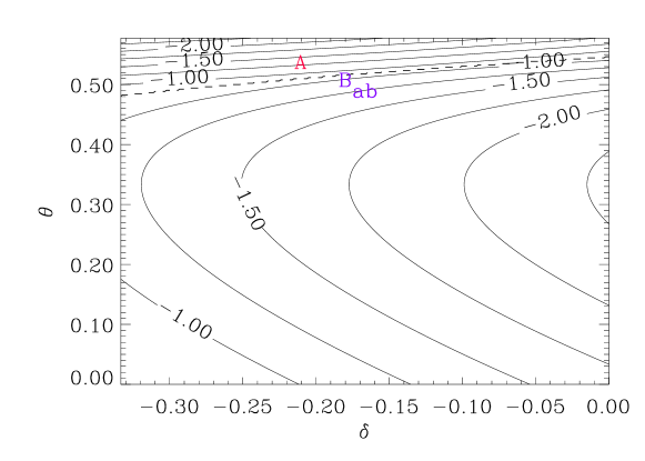
FIG. 1.: The contours delimit the values of the smallest spectral slope ${\rm min}_{j}(n_{j}^{\rm IP})$ as a function of the parameters $\delta$ and $\theta$, defined in Eqs. (8), (10). The dashed line separates the regions in which either the model-independent axion $A$ or the axion $B_{ab}$ dominates.

In Fig. 1, we show a contour plot of the smallest spectral slope ${\rm min}_{j}(n_{j}^{\rm IP})$ in the parameter space $\delta-\theta$; we recall that $\delta$ and $\theta$ characterize the evolution of external dimensions during DDI and the IP respectively [see Eqs. (8), (10)]. The dashed line separates the areas which refers to the model-independent axion $A$, and to the axion $B_{ab}$ associated to the internal components of $B_{\mu\nu}$. The spectral slope of these latter depend sensitively on the evolution of the 6 internal dimensions during DDI and IP, and in Fig. 1, we chose to show the case in which $2$ internal dimensions compactify isotropically. In the following, we will examine the various cases in which $a$ dimensions compactify isotropically, and the other $6-a$ are stabilized during DDI and IP. We find that the following two possiblities arise:

(1) if $|\delta|\sim 1/3$ and $\theta$ is close to its maximal value, which corresponds to saturation of the Kasner constraint Eq. (9), i.e. stabilized internal dimensions, then the smallest slope is negative, and is carried by $A$. In this case, the model-independent axion carries all the energy density at $\eta>\eta_{1}$. However, when one assumes that compactification is anisotropic, i.e. $a$ dimensions compactify isotropically and $6-a$ are stabilized during both DDI and IP one obtains a slightly different picture. In some cases, as the one shown in Fig. 1, the minimal slope is everywhere negative, and the bulk of the energy density is carried by either $A$ or $B_{ab}$ axions, depending on the value of $\delta$ and $\theta$.

(2) if the smallest spectral slope is positive, meaning $n_{j}^{\rm IP}>0$ for all $j$, then all fields roughly share the same energy density at time $\eta>\eta_{s}$. This case is therefore very similar to that envisaged in Section III, i.e. for a sudden branch change. Notably, one finds $Y_{m}\sim 0.3/g_{\star}$ as previously, and entropy production as before may be considered to eliminate this problem. We will thus ignore this case in the following, and rather concentrate on case (1), assuming that one of the axions dominate the energy density at time $\eta_{1}$.

In the following, we denote generically as ${\cal A}$ the axion field that carries the energy density at times $\eta>\eta_{1}$, and when necessary we will specify whether ${\cal A}$ is $A$ or $B_{ab}$. The fraction of energy density contained in species $j$ is:

$$\Omega_{j}\simeq{\cal N}_{j}\left|\frac{\eta_{1}}{\eta_{s}}\right|^{n_{\cal A}^{\rm IP}}\left[1+\left|\frac{\eta_{1}}{\eta_{s}}\right|^{-n_{j}^{\rm IP}}\right],\quad\quad\eta>\eta_{1}$$ (37)

where we used $k_{1}/k_{s}=\eta_{s}/\eta_{1}$. One can derive a relation between the duration of the “dual-dilaton” phase $|\eta_{1}/\eta_{s}|$ and the coupling constant $g_{1}$ at time $\eta_{1}$ from the criticality condition $\rho_{\cal A}\simeq\rho_{c}$, which gives:

$$\left|\frac{\eta_{1}}{\eta_{s}}\right|^{\epsilon_{\cal A}}\simeq g_{1},$$ (38)

where the exponent $\epsilon_{\cal A}=(2\theta-1)/(1-\theta)+n_{\cal A}^{\rm IP}/2$ and is negative in the region of the parameter space where $n_{\cal A}^{\rm IP}<0$. To derive Eq. (38) we used $a(\eta)\propto|\eta|^{\theta/1-\theta}$, $H\propto|\eta|^{-1/1-\theta}$ and $g\propto|\eta|^{(3\theta-1)/2(1-\theta)}$, Eq. (36), and $\rho_{c}=(3/8\pi)g_{1}^{-2}H_{1}^{2}M_{s}^{2}$ at $\eta=\eta_{1}$. If ${\cal A}$ is the model-independent axion $A$, $n_{\cal A}^{\rm IP}=4/(1-\delta)-4\theta/(1-\theta)$, while if ${\cal A}$ is a $B_{ab}$ axion, $n_{\cal A}^{\rm IP}=4-4|\beta_{a}/(1-\delta)-\xi_{a}/(1-\theta)|$, where $\beta_{a}$ and $\xi_{a}$ parametrize the evolution of the internal scale factor during DDI and the “dual-dilaton” phase, respectively; $\beta_{a}$ is tied to $\delta$ by the Kasner constraint Eq. (9) and similarly for $\xi_{a}$ as a function of $\theta$ (see Ref. [14]). Therefore Eq. (37) can be re-written as: $\Omega_{j}\simeq{\cal N}_{j}g_{1}^{n_{\cal A}^{\rm IP}/\epsilon_{\cal A}}[1+g_{1}^{-n_{j}^{\rm IP}/\epsilon_{\cal A}}]$. It is difficult to give quantitative estimates for the total fraction of energy density carried by radiation, since the various components of radiation have different spectral slopes, and some of them can be negative (see Tab. I). In the following, we thus assume that radiation can be considered, on average, as one species with number of degrees of freedom ${\cal N}_{r}\sim g_{\star}/2$ (as before), with a positive spectral slope, which implies

$$\Omega_{r}\simeq{\cal N}_{r}\,g_{1}^{n_{\cal A}^{\rm IP}/\epsilon_{\cal A}}\,.$$ (39)

Note that this number can actually be of order 1 if ${\cal N}_{r}$ is sufficiently large as compared to $g_{1}^{n_{\cal A}^{\rm IP}/\epsilon_{\cal A}}$; however, this case would be similar to a sudden branch change, since $g_{1}^{1/\epsilon_{\cal A}}\simeq|\eta_{1}/\eta_{s}|$ would be of order unity, and the results of previous sections apply. We thus assume $\Omega_{r}\ll 1$ in what follows. To be definite, let us take $g_{1}\simeq 10^{-1}$, $\theta=1/\sqrt{3}$ (corresponding to stabilized internal dimensions during IP) we find, varying $\delta$ in the range $(0,-1/3)$:

$$\frac{H_{1}}{M_{s}}\sim 10^{-7}-10^{-3}\,,\quad\quad\Omega_{r}\sim{\cal N}_{r}\,(10^{-4}-10^{-3})\,,$$ (40)

while posing $g_{1}\simeq 10^{-3}$ we get:

$$\frac{H_{1}}{M_{s}}\sim 10^{-20}-10^{-8}\,,\quad\quad\Omega_{r}\sim{\cal N}_{r}\,(10^{-12}-10^{-9})\,,$$ (41)

In contrast to the scenario with no intermediate phase, when a dual-dilaton intermediate era is present, reheating cannot be provided by gauge non-singlets, because at $\eta>\eta_{1}$ they generically carry a small amount of energy ($\Omega_{j}\ll 1$), as discussed above. Let us then investigate the possibility of reheating via the axion fields present in our PBB model. Reheating may proceed if the axion can recreate radiation by scattering or conversions with photons, that is through the processes ${\cal A}+{\cal A}\rightarrow\gamma+\gamma$ and ${\cal A}+\gamma\rightarrow{\cal A}+\gamma$. The interaction rate of the latter channel is strongly suppressed relative to the the rate of the former, since the radiation number density is small. The interaction term between ${\cal A}$ and the gauge fields is of the form $({\cal A}/M^{\prime}){\cal F}\widetilde{\cal F}$. The mass scale $M^{\prime}\simeq M_{\rm Pl}$ for the model-independent axion $A$, but $M^{\prime}$ can be different for the $B_{ab}$ axions, as it then depends on the compactification [49]. Indeed, as shown in the action Eq. (5), the coupling of $B_{ab}$ to $W\widetilde{W}$ or $V\widetilde{V}$, depends on the expectation values of the internal moduli.

The cross-section for ${\cal A}-{\cal A}$ scattering thus is of the form $\sigma\sim E_{\cal A}^{2}/M^{\prime 4}$, where the typical axion energy $E_{\cal A}\sim H_{1}(a_{1}/a)$, with $H_{1}$ possibly much smaller than $M_{s}$ for a dual-dilaton intermediate phase. Finally, the axion energy density is given by: $\rho_{\cal A}\simeq(3/8\pi)g_{1}^{-2}H_{1}^{2}M_{s}^{2}(a_{1}/a)^{4}$, so that the interaction rate for scattering gives:

$$\frac{\Gamma_{{\cal A}{\cal A}}}{H}\sim\frac{3}{8\pi}\,g_{1}^{2}\,\left(\frac{H_{1}}{M_{s}}\right)^{2}\,\left({M^{\prime}\over M_{\rm Pl}}\right)^{-4}\,\left(\frac{a_{1}}{a}\right)^{3}\,.$$ (42)

Therefore scattering by the model-independent axion cannot provide reheating, as one normally expects $H_{1}\ll M_{s}$. However, if $(M^{\prime}/M_{\rm Pl})\mathrel{\mathchoice{\lower 3.6pt\vbox{\halign{$\mathsurround=0pt\displaystyle\hfil#\hfil$\cr<\crcr\sim\crcr}}}{\lower 3.6pt\vbox{\halign{$\mathsurround=0pt\textstyle\hfil#\hfil$\cr<\crcr\sim\crcr}}}{\lower 3.6pt\vbox{\halign{$\mathsurround=0pt\scriptstyle\hfil#\hfil$\cr<\crcr\sim\crcr}}}{\lower 3.6pt\vbox{\halign{$\mathsurround=0pt\scriptscriptstyle\hfil#\hfil$\cr<\crcr\sim\crcr}}}}g_{1}^{1/2}(H_{1}/M_{s})^{1/2}$, then $B_{ab}-B_{ab}$ axion scattering will produce radiation and reheat the Universe.

If axion scattering is ineffective, reheating may still occur through axion decay, provided the axion mass is large enough to avoid problems associated with too low a reheating temperature. A typical axion lifetime is $\tau_{\cal A}\sim M^{\prime 2}/m_{\cal A}^{3}$, where $m_{\cal A}\sim\Lambda^{3}/M_{\rm Pl}M^{\prime}$ is the axion mass (neglecting fudge factors) [49], and $\Lambda$ denotes the highest scale at which gauge interactions to which ${\cal A}$ couples become strong. In particular, for $\Lambda\sim 10^{14}\,$GeV, corresponding to phenomenologically favoured scales of gaugino condensation in a hidden sector, $m_{\cal A}\sim 10^{6}(M^{\prime}/0.01M_{\rm Pl})^{-1}\,$GeV and $\tau_{\cal A}\sim 3\times 10^{-8}\,{\rm s}\,(M^{\prime}/0.01M_{\rm Pl})^{5}$, and the reheating temperature is $T_{\rm RH}\sim 10\,{\rm GeV}\,g_{\star{\rm RH}}^{-1/4}(M^{\prime}/0.01M_{\rm Pl})^{-5/2}$. In the following subsections, we will discuss the implications of this on the moduli and gravitino problems.

B Dangerous relics

The estimate of the abundance $Y_{m}$ of moduli produced gravitationally can be obtained using the same methods as for the no-intermediate phase case. One actually finds the same result $Y_{m}\sim 0.3/g_{\star}$. This is due to the fact that the spectral slope of the energy distribution of moduli and radiation is positive for all $k$ momenta (see Tab. I), and therefore the number density of moduli $n_{m}\sim(2\pi)^{-3/2}H_{s}^{3/2}(a/a_{s})^{-3}$, where we used Eq. (34), and $n_{m}\sim\rho_{m}/E_{m}$, with $E_{m}\sim H_{s}(a/a_{s})^{-1}$ the typical moduli energy. One can also express the entropy density $s\sim g_{\star}^{1/4}\rho_{r}^{3/4}$ in a similar way, and obtain the above result for $Y_{m}$.

Just as in the no-intermediate phase case, one does not expect gravitinos to be produced gravitationally in the dual-dilaton phase if they are effectively massless. However, even if radiation has not thermalized, they can be produced by scattering during the dual-dilaton phase. Since the string coupling (hence the production cross-section) evolves with time during dual-dilaton phase, it is more convenient to write the Boltzmann equation in terms of conformal time, which when disregarding annihilations channels gives:

$$\frac{dY_{3/2}^{s}}{d\eta}=\Sigma_{\rm tot}\,s\,a\,Y_{a}^{2}\,,\quad\quad\eta_{s}<\eta,$$ (43)

where we recall that the scale factor $a\propto|\eta|^{\theta/(1-\theta)}$ during the IP, $s\propto a^{-3}$, and $\Sigma_{\rm tot}\sim 500g^{4}/M_{s}^{2}$, and as before $Y_{a}\sim 0.3/g_{\star}$ denotes the ratio of number density to entropy density of radiation quanta per helicity state. Using $g^{2}\propto|\eta|^{(3\theta-1)/(1-\theta)}$ during the IP, one easily obtains as before $Y_{3/2}^{s}=Y_{a}\Gamma/H$, with $\Gamma\sim\Sigma_{\rm tot}Y_{a}s$ the gravitino production rate, and the right hand side should be evaluated at time $\eta_{1}$ if $\theta>1/3$, and at time $\eta_{s}$ if $\theta<1/3$.

Thus, using $(\Sigma_{\rm tot}s/H)_{\eta_{1}}\sim 70g_{1}^{5/2}\,g_{\star}^{1/4}\,\Omega_{r}^{3/4}(H_{1}/M_{s})^{1/2}$, and Eq. (39), one finally obtains:

$$Y_{3/2}\sim 6g_{\star}^{-1}\,g_{1}^{\kappa}\,\left(\frac{H_{s}}{M_{s}}\right)^{1/2}\,,$$ (44)

with:

$$\theta>1/3:\quad\kappa={5\over 2}-{1\over 2\epsilon_{\cal A}(1-\theta)}+{3n^{\rm IP}_{\cal A}\over 4\epsilon_{\cal A}}\,,$$ (45)

$$\theta<1/3:\quad\kappa={5\over 2}-{1\over 2\epsilon_{\cal A}(1-\theta)}+{3n^{\rm IP}_{\cal A}\over 4\epsilon_{\cal A}}+{1-3\theta\over\epsilon_{\cal A}(1-\theta)}\,.$$ (46)

Let us first observe that, if $\theta<1/3$ the coupling $g$ decreases in time during the IP (see Eq. (9)). In the scenario under investigation, i.e. with a dual-dilaton intermediate phase, it is assumed that quantum string-loop effects are never operative ($g<1$) and that because of high-curvature corrections the Hubble-parameter makes a bounce around its maximal value at the string scale. If we impose that the dilaton field reaches the present value at the end of the PBB era, unless we assume either an extremely low decreasing of the coupling during the IP or a very short intermediate phase (which would give for $Y_{3/2}^{s}$ roughly the same value as in the scenario with no-intermediate phase), we are forced to limit to the region of parameter space where $\theta>1/3$. Having restricted ourselves to the case described by Eq. (45), we find that the exponent $\kappa$ takes values between $\sim 2$ and $\sim 9$ depending on the evolution of internal dimensions, and therefore, $Y_{3/2}\sim 10^{-4}\to 10^{-10}$ for $g_{1}\sim 0.1$, $g_{\star}\sim 100$. For anisotropic compactification, in some region of the parameter space, one finds even higher values of $\kappa$, for which there would be no gravitino problem at all. One thus finds that in the presence of a dual-dilaton phase, the gravitino is generically less efficiently produced (possibly much less) than in the no-intermediate phase case. This can be understood in the following way. If $\theta>1/3$, the string coupling grows during IP, so that the cross-section $\Sigma_{\rm tot}\propto g^{4}$ is very small at the beginning of the dual-dilaton phase, and gravitino production takes place at Hubble scale $H_{1}$. However, unlike the no-intermediate phase case, here one generically has $H_{1}\ll H_{s}\sim M_{s}$, and therefore gravitino production is inefficient. Finally, the small number density of radiation quanta (recall $\Omega_{r}\ll 1$) also hampers gravitino production in this case.

C Sources of entropy and baryogenesis

Due to the overproduction of moduli (and possibly gravitinos), entropy production is still necessary in the present scenario. Entropy production is also necessary if the axion cannot reheat the Universe, e.g. if its coupling to the gauge fields is too weak, and its mass too small. However, there are several possible sources of entropy production, as we now discuss.

If the axion field dominates the energy density at the beginning of the radiation era and it reheats the Universe through scattering or decay, reheating is accompanied by entropy production to the level of $\Delta s\sim(\rho_{\cal A}/\rho_{r})^{3/4}$, where $\rho_{\cal A}$ and $\rho_{r}$ denote the energy density contained in the axion and in radiation at reheating. If the axion is still relativistic at that time, i.e. if it reheats the Universe through scattering at high energy scale, then $\Delta s\sim\Omega_{r}^{-3/4}$, where $\Omega_{r}$ is defined as before at time $\eta_{1}$. The moduli abundance would be reduced to $Y_{m}\sim 0.3g_{\star}^{-1}\,\Omega_{r}^{3/4}$ and to obtain $Y_{m}\mathrel{\mathchoice{\lower 3.6pt\vbox{\halign{$\mathsurround=0pt\displaystyle\hfil#\hfil$\cr<\crcr\sim\crcr}}}{\lower 3.6pt\vbox{\halign{$\mathsurround=0pt\textstyle\hfil#\hfil$\cr<\crcr\sim\crcr}}}{\lower 3.6pt\vbox{\halign{$\mathsurround=0pt\scriptstyle\hfil#\hfil$\cr<\crcr\sim\crcr}}}{\lower 3.6pt\vbox{\halign{$\mathsurround=0pt\scriptscriptstyle\hfil#\hfil$\cr<\crcr\sim\crcr}}}}10^{-13}$, one needs $\Omega_{r}\mathrel{\mathchoice{\lower 3.6pt\vbox{\halign{$\mathsurround=0pt\displaystyle\hfil#\hfil$\cr<\crcr\sim\crcr}}}{\lower 3.6pt\vbox{\halign{$\mathsurround=0pt\textstyle\hfil#\hfil$\cr<\crcr\sim\crcr}}}{\lower 3.6pt\vbox{\halign{$\mathsurround=0pt\scriptstyle\hfil#\hfil$\cr<\crcr\sim\crcr}}}{\lower 3.6pt\vbox{\halign{$\mathsurround=0pt\scriptscriptstyle\hfil#\hfil$\cr<\crcr\sim\crcr}}}}10^{-13}$. One can check that such a low value of $\Omega_{r}$ cannot be obtained for realistic values with $g_{1}\,\raise 1.72218pt\hbox{$>$}\kern-6.99997pt\lower 2.6694pt\hbox{$\sim$}\,10^{-3}$ in the parameter space defined by $\delta$ and $\theta$, using the results so far obtained for the axion $B_{ab}$ (recall that the axion $A$ cannot reheat by scattering). For example, in the case of the axion $B_{ab}$ with only 2 internal dimensions compactified and the other 4 stabilized, the smallest value of $\Omega_{r}$ for $g_{1}\,\raise 1.72218pt\hbox{$>$}\kern-6.99997pt\lower 2.6694pt\hbox{$\sim$}\,10^{-3}$ is actually $\Omega_{r}\sim 10^{-6}$, with ${\cal N}_{r}\sim 100$, which would imply $Y_{m}\sim 10^{-7}$ at the end of reheating and entropy production is still necessary. Moreover, note that $\Omega_{r}\sim 10^{-6}$ also corresponds to $H_{1}\sim 10^{-13}M_{s}$, hence $M^{\prime}/M_{\rm Pl}\sim 10^{-8}$, which is a rather strong requirement on $M^{\prime}$. Nevertheless, one should recall at this stage that the domination and decay of an Affleck-Dine flat direction would lead to further entropy production $\Delta s^{\prime}\sim 10^{6}$ [see Eq. (28)]. Thus one could actually dilute the moduli and gravitinos down to acceptable levels with an Affleck-Dine condensate only (no $\chi$ modulus). This would however produce too large a baryon asymmetry, $n_{\rm B}/s\sim{\cal O}(1)$, unless the $CP$ violation parameter is very small and/or electroweak baryon number erasure is very efficient [47].

Let us now consider the alternate case, in which the axion acquires a large mass, and later decays to radiation. Entropy production then results from the decay of the axion oscillations around the minimum of its potential, whose generic form [49] is $V({\cal A})\sim(\Lambda^{6}/M_{\rm Pl}^{2})\,\left[1-{\rm cos}\left({\cal A}/F\right)\right]$, with $F\sim M^{\prime}/\pi^{2}$ the axion decay constant. The axion vev ${\cal A}_{0}$ is in fact generically displaced by $\sim M^{\prime}/\pi$ from its true minimum, and its coherent oscillations and decay will produce entropy. Using the results of Section III, one can easily obtain:

$$\Delta s\simeq 10^{7}\,\left(\frac{{\cal A}_{0}}{M^{\prime}}\right)^{2}\,\left(\frac{M^{\prime}}{0.01M_{\rm Pl}}\right)^{4}\,\left(\frac{\Lambda}{10^{14}\,{\rm GeV}}\right)^{-3}\,\Omega_{r}^{-3/4}\,.$$ (47)

The amount of entropy produced is only marginally sufficient, but it depends in a sensitive way on $\Lambda$ and $\Omega_{r}$. For smaller values of the gaugino condensation scale, say $\Lambda\sim\,{\rm few}\times 10^{13}\,$GeV, and, say $\Omega_{r}\mathrel{\mathchoice{\lower 3.6pt\vbox{\halign{$\mathsurround=0pt\displaystyle\hfil#\hfil$\cr<\crcr\sim\crcr}}}{\lower 3.6pt\vbox{\halign{$\mathsurround=0pt\textstyle\hfil#\hfil$\cr<\crcr\sim\crcr}}}{\lower 3.6pt\vbox{\halign{$\mathsurround=0pt\scriptstyle\hfil#\hfil$\cr<\crcr\sim\crcr}}}{\lower 3.6pt\vbox{\halign{$\mathsurround=0pt\scriptscriptstyle\hfil#\hfil$\cr<\crcr\sim\crcr}}}}10^{-2}$, reasonable values of $\Delta s\mathrel{\mathchoice{\lower 3.6pt\vbox{\halign{$\mathsurround=0pt\displaystyle\hfil#\hfil$\cr>\crcr\sim\crcr}}}{\lower 3.6pt\vbox{\halign{$\mathsurround=0pt\textstyle\hfil#\hfil$\cr>\crcr\sim\crcr}}}{\lower 3.6pt\vbox{\halign{$\mathsurround=0pt\scriptstyle\hfil#\hfil$\cr>\crcr\sim\crcr}}}{\lower 3.6pt\vbox{\halign{$\mathsurround=0pt\scriptscriptstyle\hfil#\hfil$\cr>\crcr\sim\crcr}}}}10^{10}$ may be achieved. Note that baryogenesis can be implemented in the very same way as in Section III in this context.

One should recognize that the above estimates remain somehow qualitative, since they make particular assumptions on the axion couplings, and therefore on the compactification process, whereas we assumed a simple toroidal compactification. Nevertheless, our aim here is to show that there exists various possibilities to generate entropy to the level required.

Even if axions cannot reheat the Universe through scattering or decay, one may still consider the mechanism discussed in Section III, where a modulus (the dilaton?) of mass $\sim 10^{6}\,$GeV reheats through the decay of its coherent oscillations. The discussion is similar to that of Section III, up to the fact that there may be no radiation dominated era preceeding the $\chi$ dominated era, if $H_{1}\mathrel{\mathchoice{\lower 3.6pt\vbox{\halign{$\mathsurround=0pt\displaystyle\hfil#\hfil$\cr<\crcr\sim\crcr}}}{\lower 3.6pt\vbox{\halign{$\mathsurround=0pt\textstyle\hfil#\hfil$\cr<\crcr\sim\crcr}}}{\lower 3.6pt\vbox{\halign{$\mathsurround=0pt\scriptstyle\hfil#\hfil$\cr<\crcr\sim\crcr}}}{\lower 3.6pt\vbox{\halign{$\mathsurround=0pt\scriptscriptstyle\hfil#\hfil$\cr<\crcr\sim\crcr}}}}H_{\rm dom}$ ($H_{\rm dom}$ denotes as before the Hubble scale at which $\chi$ comes to dominate the energy density), i.e. if the dual-dilaton era ends as $\chi$ dominates. However, as we now argue, this does not happen, and one always has $H_{1}\gg H_{\rm dom}$. Following the discussion of Section III to calculate $H_{\rm dom}$, using $a\propto H^{-\theta}$ in the IP era, one finds: $H_{\rm dom}\sim m_{\chi}[(8\pi/3)(g_{1}\chi_{0}/M_{s})]^{2/(2-3\theta)}$, where $g_{1}$ is the value of the string coupling at Hubble scale $H_{\rm dom}$, which marks the end of IP. In the absence of the $\chi$ modulus, the transition to the radiation dominated era would take place at $H_{1}\sim H_{s}g_{1}^{-1/\epsilon_{\cal A}(1-\theta)}$ [see Eq. (38)]. We consider that in either case, the value of the string coupling at the end of the IP, i.e. at $H_{\rm dom}$ or at $H_{1}$, should be close to its present value. One then must determine whether or not $H_{\rm dom}\mathrel{\mathchoice{\lower 3.6pt\vbox{\halign{$\mathsurround=0pt\displaystyle\hfil#\hfil$\cr<\crcr\sim\crcr}}}{\lower 3.6pt\vbox{\halign{$\mathsurround=0pt\textstyle\hfil#\hfil$\cr<\crcr\sim\crcr}}}{\lower 3.6pt\vbox{\halign{$\mathsurround=0pt\scriptstyle\hfil#\hfil$\cr<\crcr\sim\crcr}}}{\lower 3.6pt\vbox{\halign{$\mathsurround=0pt\scriptscriptstyle\hfil#\hfil$\cr<\crcr\sim\crcr}}}}H_{1}$, and it can be checked that for nearly all values of the $\delta-\theta$ parameters, we have indeed $H_{\rm dom}\ll H_{1}$. The dual-dilaton phase thus ends before and radiation domination occurs before $\chi$ dominates. All estimates made in Section III can thus be directly applied to the present case. It is interesting to note that here, one generically has $\Omega_{r}\ll 1$ (the “radiation dominated” era is driven by ${\cal A}$), and therefore entropy production is more efficient by a factor $\Omega_{r}^{-3/4}\sim 10-10^{6}$, for ${\cal N}_{r}\sim 100$ and $g_{1}\sim 0.001-0.1$. The amount of moduli present at $\chi$ decay is thus further reduced by this factor. The monopole abundance today is also reduced by a factor $\Omega_{r}^{-1/4}\sim 2-100$ [see Eq. (25)]. Baryogenesis can be implemented as before via the Affleck-Dine mechanism, and the baryon asymmetry is given by Eq. (33).

In fact, if $\Omega_{r}\mathrel{\mathchoice{\lower 3.6pt\vbox{\halign{$\mathsurround=0pt\displaystyle\hfil#\hfil$\cr<\crcr\sim\crcr}}}{\lower 3.6pt\vbox{\halign{$\mathsurround=0pt\textstyle\hfil#\hfil$\cr<\crcr\sim\crcr}}}{\lower 3.6pt\vbox{\halign{$\mathsurround=0pt\scriptstyle\hfil#\hfil$\cr<\crcr\sim\crcr}}}{\lower 3.6pt\vbox{\halign{$\mathsurround=0pt\scriptscriptstyle\hfil#\hfil$\cr<\crcr\sim\crcr}}}}10^{-6}$, entropy production to the level of $\Delta s\mathrel{\mathchoice{\lower 3.6pt\vbox{\halign{$\mathsurround=0pt\displaystyle\hfil#\hfil$\cr>\crcr\sim\crcr}}}{\lower 3.6pt\vbox{\halign{$\mathsurround=0pt\textstyle\hfil#\hfil$\cr>\crcr\sim\crcr}}}{\lower 3.6pt\vbox{\halign{$\mathsurround=0pt\scriptstyle\hfil#\hfil$\cr>\crcr\sim\crcr}}}{\lower 3.6pt\vbox{\halign{$\mathsurround=0pt\scriptscriptstyle\hfil#\hfil$\cr>\crcr\sim\crcr}}}}10^{6}$ would be sufficient to dilute the moduli and gravitinos to acceptable levels, and such entropy could be provided by the Affleck-Dine condensate, in the absence of any $\chi$ modulus. It should be noted, however, that such low values of $\Omega_{r}$ only arise when $g_{1}\mathrel{\mathchoice{\lower 3.6pt\vbox{\halign{$\mathsurround=0pt\displaystyle\hfil#\hfil$\cr<\crcr\sim\crcr}}}{\lower 3.6pt\vbox{\halign{$\mathsurround=0pt\textstyle\hfil#\hfil$\cr<\crcr\sim\crcr}}}{\lower 3.6pt\vbox{\halign{$\mathsurround=0pt\scriptstyle\hfil#\hfil$\cr<\crcr\sim\crcr}}}{\lower 3.6pt\vbox{\halign{$\mathsurround=0pt\scriptscriptstyle\hfil#\hfil$\cr<\crcr\sim\crcr}}}}10^{-2}$.

As a conclusion, when either $A$ or $B_{ab}$ axions dominate the energy density at the end of a dual-dilaton intermediate phase, there are various natural sources of entropy: axion scattering, axion decay, or domination and the decay of a modulus or an Affleck-Dine condensate. Since one generically has $\Omega_{r}\ll 1$, entropy production is more efficient than in the absence of an intermediate phase, and both moduli and monopoles can be diluted down to low levels. In some cases, the Affleck-Dine condensate provides enough entropy by itself to solve the moduli/gravitino problem, although one then has to cope with a very large baryon asymmetry from the decay of the condensate.

VI “String” intermediate phase and black holes

During the string era, modes exit and do not re-enter the horizon. Therefore $k_{s}<k_{1}$, and one expects to produce one particle per mode at $k_{1}$ since it exits the horizon and re-enters at the same absolute value of conformal time.

However, the situation here is more delicate than in the case of the dual-dilaton phase. Indeed, a mode that exits the horizon at conformal time $\eta_{\rm ex}$, with $\eta_{\rm ex}<0$ in the present scenario, will re-enter at time $\eta_{\rm re}\simeq|\eta_{\rm ex}|$ (if $\eta_{\rm ex}\ll\eta_{1}$, i.e. if the mode exits well before the end of the “string” phase). This means that at time $\eta_{1}$, which is supposed to mark the start of the FRW regime, only those modes with wavenumber $\sim k_{1}$, i.e. the highest frequencies, have re-entered. The modes that exited the horizon at the beginning of the “string” phase (wavenumber $\sim k_{s}$) will re-enter later, possibly much later, at conformal time $|\eta_{s}|\gg|\eta_{1}|$. One can rewrite the energy density Eq. (12) in this scenario, at time $\eta$ with $\eta_{1}<\eta<|\eta_{s}|$, which gives:

$$\rho_{j}(\eta)\simeq\frac{{\cal N}_{j}}{2\pi^{2}}H_{1}^{4}\,\left(\frac{a_{1}}{a}\right)^{4}\,\left|1-\left|\frac{\eta}{\eta_{1}}\right|^{-n_{j}^{\rm IP}}\right|\quad\quad\eta_{1}<\eta<|\eta_{s}|\,,$$ (48)

and as before, we imposed a low wavenumber cut-off at the horizon size $\sim 1/\eta$. In the case of the “string” phase, inspection of Table I reveals that the model-independent axion has the most negative slope $=-2\zeta$ ($\zeta>0$), and its energy density $\rho_{A}\sim({\cal N}_{A}/2\pi^{2})H_{1}^{4}a_{1}^{4}|\eta/\eta_{1}|^{2\zeta}/a^{4}$. At time $\eta_{1}$, only modes with wavenumber $k_{1}$ have re-entered, so within the horizon, all fields share roughly the same energy density. However, as time goes beyond $\eta_{1}$, the axion will quickly come to dominate the energy density. Assuming the dilaton field is fixed for $\eta>\eta_{1}$, since $H^{2}\propto\rho_{A}$, and $H=a^{\prime}/a^{2}$, it is straightforward to derive that $a\propto\eta^{1+\zeta}$. In this case, with $\zeta>0$, the dynamics is driven by the axion fluctuations. This is inconsistent since the gravitational amplification of these fluctuations, in particular the spectral slope of the axion, were calculated assuming that the fluctuations would re-enter during a radiation dominated era, and with $\zeta>0$, the expression for the scale factor shows that this is not the case.

This inconsistency reflects the breakdown of the perturbative approach used to calculate the amplification of axion fluctuations. In effect, the calculation assumes that the quantum fluctuations can be treated as a perturbation on a fixed classical background, whereas in the present case, one should consider their back-reaction effect on the background spacetime. Moreover, since the axion field is assumed not to participate to the dynamics, its classical vev is zero, and the energy density stored in axion is $\rho_{A}\sim(\partial\delta A)^{2}$, where $\delta A$ represents the fluctuation in the axion field. One should therefore include back-reaction up to second order in the fluctuations, in order to derive the dynamics of the era between times $\eta_{1}$ and $|\eta_{s}|$, and such an intricate calculation is well beyond the scope of the present paper. Note, however, that the above inconsistency does not arise for conformal times $\eta>|\eta_{s}|$, since $n_{j}^{\rm DDI}>0$ for all $j$, and radiation domination should be a valid approximation.

We thus consider, as an alternative, that black holes form on all scales comprised between $k_{1}$ and $k_{s}$. This is a possible outcome of the above dynamics, as black holes generically form copiously when relative overdensities of order unity re-enter the horizon. At late times $\eta>|\eta_{s}|$, the Universe will be dominated by those black holes that have not evaporated yet. The lifetime of a black hole $\tau_{\rm bh}\propto M_{\rm bh}^{3}\propto H_{i}^{-3}$, where $M_{\rm bh}$ denotes the black hole mass, and corresponds to the mass within the horizon at the time of formation at Hubble scale $H_{i}$. Therefore the Universe will be dominated by those black holes that formed last, i.e. on scale $k_{s}$, and will reheat with the evaporation of those black holes. The Hubble scale $H(|\eta_{s}|)\sim H_{1}|\eta_{s}/\eta_{1}|^{-3/2}$ if the era between times $\eta_{1}$ and $|\eta_{s}|$ is matter dominated (black hole domination). Then $M_{\rm bh}\sim 4\pi m_{\rm Pl}[H(|\eta_{s}|)/m_{\rm Pl}]^{-1}$ (which corresponds to the mass within the horizon at that time) and the evaporation timescale of those black holes reads $\tau_{\rm bh}\sim m_{\rm Pl}^{-1}(M_{\rm bh}/m_{\rm Pl})^{3}\sim(4\pi)^{3}m_{\rm Pl}^{-1}[H(|\eta_{s}|)/m_{\rm Pl}]^{-3}$, so that the black holes evaporate and reheat the Universe at a Hubble scale $H_{\rm ev}\sim(4\pi)^{-3}H(|\eta_{s}|)[H(|\eta_{s}|)/m_{\rm Pl}]^{2}$.

Such reheating by black hole evaporation was envisaged in Ref. [50] in the context of the PBB scenario. Note that it is accompanied by entropy production, to the level of $\Delta s\sim(\rho_{\rm BH}/\rho_{r})^{3/4}$, where $\rho_{\rm BH}$ and $\rho_{r}$ denote the energy densities contained in black holes and in radiation at the time of evaporation. This entropy production can be rewritten as $\Delta s\sim 10^{19}\,g_{1}^{1/2}\Omega_{r}^{-3/4}[H(|\eta_{s}|)/10^{7}\,{\rm GeV}]^{-3/2}(H_{1}/M_{s})^{1/2}$, and the reheating temperature $T_{\rm RH}\sim 0.6\,{\rm GeV}\,[H(|\eta_{s}|)/10^{7}\,{\rm GeV}]^{3/2}$. Even though this entropy production may be sufficiently large to dilute the moduli created gravitationally during the DDI and “string” phases, the same moduli are also part of the Hawking radiation of the evaporating black holes. The number density to entropy density ratio of moduli and gravitinos present after evaporation in fact reads [51]: $Y_{m}\sim 10^{-9}[H(|\eta_{s}|)/10^{7}\,{\rm GeV}]^{1/2}$, assuming $g_{\star}\sim 200$ at evaporation. Clearly, black hole evaporation eliminates one moduli problem, to reintroduce another, and further entropy production is necessary.

Consider then a modulus $\chi$ as introduced in Section IV.A, with mass $m_{\chi}$. The amount of entropy produced by $\chi$ is given in Eq. (22). However, if black holes have not evaporated by the time $\chi$ would dominate (if black holes were absent), the r.h.s of Eq. (22) should be multiplied by $(H_{\rm ev}/H_{\rm dom})^{1/2}$, where $H_{\rm dom}\sim m_{\chi}(\chi_{0}/m_{\rm Pl})^{4}$ corresponds to the Hubble scale at which $\chi$ would dominate in the absence of black holes. Using $H_{\rm ev}\sim 10^{6}\,{\rm GeV}[H(|\eta_{s}|)/2\cdot 10^{15}\,{\rm GeV})]^{3}$, and assuming $H_{\rm ev}\mathrel{\mathchoice{\lower 3.6pt\vbox{\halign{$\mathsurround=0pt\displaystyle\hfil#\hfil$\cr<\crcr\sim\crcr}}}{\lower 3.6pt\vbox{\halign{$\mathsurround=0pt\textstyle\hfil#\hfil$\cr<\crcr\sim\crcr}}}{\lower 3.6pt\vbox{\halign{$\mathsurround=0pt\scriptstyle\hfil#\hfil$\cr<\crcr\sim\crcr}}}{\lower 3.6pt\vbox{\halign{$\mathsurround=0pt\scriptscriptstyle\hfil#\hfil$\cr<\crcr\sim\crcr}}}}H_{\rm dom}$, the final moduli abundance is:

$$Y_{m}\sim 10^{-17}\,\gamma_{\chi}^{1/2}\,\left(\frac{m_{\chi}}{10^{6}\,{\rm GeV}}\right)^{3/2}\,\left(\frac{H(|\eta_{s}|)}{2\cdot 10^{15}\,{\rm GeV}}\right)^{-1}\,\Omega_{r}^{3/4}\,,$$ (49)

hence, for $H_{1}\sim 10^{17}\,$GeV, provided the phase in which black holes dominate does not last too long, i.e. $|\eta_{s}/\eta_{1}|\mathrel{\mathchoice{\lower 3.6pt\vbox{\halign{$\mathsurround=0pt\displaystyle\hfil#\hfil$\cr<\crcr\sim\crcr}}}{\lower 3.6pt\vbox{\halign{$\mathsurround=0pt\textstyle\hfil#\hfil$\cr<\crcr\sim\crcr}}}{\lower 3.6pt\vbox{\halign{$\mathsurround=0pt\scriptstyle\hfil#\hfil$\cr<\crcr\sim\crcr}}}{\lower 3.6pt\vbox{\halign{$\mathsurround=0pt\scriptscriptstyle\hfil#\hfil$\cr<\crcr\sim\crcr}}}}4\times 10^{3}$, then $H(|\eta_{s}|)\mathrel{\mathchoice{\lower 3.6pt\vbox{\halign{$\mathsurround=0pt\displaystyle\hfil#\hfil$\cr>\crcr\sim\crcr}}}{\lower 3.6pt\vbox{\halign{$\mathsurround=0pt\textstyle\hfil#\hfil$\cr>\crcr\sim\crcr}}}{\lower 3.6pt\vbox{\halign{$\mathsurround=0pt\scriptstyle\hfil#\hfil$\cr>\crcr\sim\crcr}}}{\lower 3.6pt\vbox{\halign{$\mathsurround=0pt\scriptscriptstyle\hfil#\hfil$\cr>\crcr\sim\crcr}}}}4\times 10^{11}\,{\rm GeV}$ and $Y_{m}\mathrel{\mathchoice{\lower 3.6pt\vbox{\halign{$\mathsurround=0pt\displaystyle\hfil#\hfil$\cr<\crcr\sim\crcr}}}{\lower 3.6pt\vbox{\halign{$\mathsurround=0pt\textstyle\hfil#\hfil$\cr<\crcr\sim\crcr}}}{\lower 3.6pt\vbox{\halign{$\mathsurround=0pt\scriptstyle\hfil#\hfil$\cr<\crcr\sim\crcr}}}{\lower 3.6pt\vbox{\halign{$\mathsurround=0pt\scriptscriptstyle\hfil#\hfil$\cr<\crcr\sim\crcr}}}}10^{-13}$.

To summarize, black hole reheating of the PBB scenario, as envisaged in Ref. [50], does not solve the moduli problem; it also requires another source of entropy production, and the oscillations and decay of the $\chi$ modulus would be sufficient, provided the “string” phase does not last more than $\sim 8$ e–folds of the scale factor. In this case, baryogenesis could also be implemented as in Section IV.B.

VII Discussions and conclusions

We find that pre-big bang cosmological models inevitably face a severe gravitino/moduli problem, as they predict a number density to entropy density ratio of gravitationally produced moduli at the beginning of the radiation era of the order of $Y_{m}\sim 0.3/g_{\star}$, where $g_{\star}$ counts the number of degrees of freedom in the radiation bath at that time. These models also predict a similar amount of gravitinos, albeit somewhat smaller if gravitinos are not produced gravitationally during dilaton driven inflation, yet far in excess of the BBN bounds $Y_{m,3/2}\mathrel{\mathchoice{\lower 3.6pt\vbox{\halign{$\mathsurround=0pt\displaystyle\hfil#\hfil$\cr<\crcr\sim\crcr}}}{\lower 3.6pt\vbox{\halign{$\mathsurround=0pt\textstyle\hfil#\hfil$\cr<\crcr\sim\crcr}}}{\lower 3.6pt\vbox{\halign{$\mathsurround=0pt\scriptstyle\hfil#\hfil$\cr<\crcr\sim\crcr}}}{\lower 3.6pt\vbox{\halign{$\mathsurround=0pt\scriptscriptstyle\hfil#\hfil$\cr<\crcr\sim\crcr}}}}10^{-13}$.

Late entropy production, to the level of $\Delta s\mathrel{\mathchoice{\lower 3.6pt\vbox{\halign{$\mathsurround=0pt\displaystyle\hfil#\hfil$\cr>\crcr\sim\crcr}}}{\lower 3.6pt\vbox{\halign{$\mathsurround=0pt\textstyle\hfil#\hfil$\cr>\crcr\sim\crcr}}}{\lower 3.6pt\vbox{\halign{$\mathsurround=0pt\scriptstyle\hfil#\hfil$\cr>\crcr\sim\crcr}}}{\lower 3.6pt\vbox{\halign{$\mathsurround=0pt\scriptscriptstyle\hfil#\hfil$\cr>\crcr\sim\crcr}}}}10^{5}-10^{10}$ depending on the details of the transition between the pre-big bang inflationary era and the radiation phase, is thus mandatory in the scenarios we have investigated. For the simplest pre-big bang model in which the transition is sudden, the amount of entropy needed is $\Delta s\mathrel{\mathchoice{\lower 3.6pt\vbox{\halign{$\mathsurround=0pt\displaystyle\hfil#\hfil$\cr>\crcr\sim\crcr}}}{\lower 3.6pt\vbox{\halign{$\mathsurround=0pt\textstyle\hfil#\hfil$\cr>\crcr\sim\crcr}}}{\lower 3.6pt\vbox{\halign{$\mathsurround=0pt\scriptstyle\hfil#\hfil$\cr>\crcr\sim\crcr}}}{\lower 3.6pt\vbox{\halign{$\mathsurround=0pt\scriptscriptstyle\hfil#\hfil$\cr>\crcr\sim\crcr}}}}10^{10}$ and this is a strong requirement. However, sufficient entropy can be produced by the domination and decay of the zero-mode of a modulus field with mass $\sim 10^{6}\,$GeV, initially displaced from the minimum of its potential by an amount $M_{s}$. The Universe will start the FRW radiation era with a temperature $T_{\rm RH}\sim 1\,{\rm GeV}$ (see Eq. (23)). Moreover, the dilaton, which drives the pre-big bang dynamics, could also play the role of this modulus, as several scenarios of gaugino condensation predict a dilaton mass $\sim 10^{6}\,$GeV, and since it can be generically displaced from its present value at the end of the pre-big bang inflation. Furthermore, this vast amount of entropy produced helps set the Affleck-Dine mechanism of baryogenesis in a natural framework, as it reduces efficiently the baryon asymmetry created in the decay of the baryon number carrying flat direction. Finally, it may also solve the usual monopole problem associated with GUT symmetry breaking, although this depends sensitively on the details of monopole formation at the GUT phase transition.

We also examined variants of the pre-big bang model in which an intermediate phase of dynamics motivated by physics at high curvature takes place between the pre-big bang inflationary phase and the radiation era. In the case of the so-called dual-dilaton intermediate phase, one finds that the moduli/gravitino problem is still present, and entropy production is still necessary. However the problem of entropy production is relieved by the small fraction of energy density contained in radiation at the beginning of the radiation era. In effect, the energy density is generically contained in an axion field, either the model-independent axion $A$ or internal axions $B_{ab}$ associated with the compactified components of $B_{\mu\nu}$. One can show that several natural sources of entropy may alleviate or solve the moduli/gravitino problem, notably the entropy produced in axion reheating via scattering (provided the axion decay constant $F\mathrel{\mathchoice{\lower 3.6pt\vbox{\halign{$\mathsurround=0pt\displaystyle\hfil#\hfil$\cr<\crcr\sim\crcr}}}{\lower 3.6pt\vbox{\halign{$\mathsurround=0pt\textstyle\hfil#\hfil$\cr<\crcr\sim\crcr}}}{\lower 3.6pt\vbox{\halign{$\mathsurround=0pt\scriptstyle\hfil#\hfil$\cr<\crcr\sim\crcr}}}{\lower 3.6pt\vbox{\halign{$\mathsurround=0pt\scriptscriptstyle\hfil#\hfil$\cr<\crcr\sim\crcr}}}}10^{-3}M_{\rm Pl}$), or that produced in oscillations and decay of the zero-mode of the dominating axion, if the axion decay constant $\sim 10^{-3}M_{\rm Pl}$ and its potential is generated by gaugino condensation in a hidden sector at scale $\Lambda\sim\,{\rm few}\times 10^{13}\,$GeV. In some regions of parameter space (which parametrizes the evolution of internal and external dimensions), the amount of entropy needed to reduce the moduli/gravitino problem is sufficiently small ($\Delta s\sim 10^{6}$) that the domination and decay of an Affleck-Dine condensate can produce both the entropy and the baryon asymmetry of the Universe. In this case the hot big bang, which marks the beginning of the FRW radiation era, takes place at a temperature $T_{\rm RH}\sim 10^{5}\,{\rm GeV}$ (see Eq. (29)).

In the case of the so-called “string” intermediate phase, one is at present unable to specify the dynamics of the era that follows the string phase (see Section VI). However, as we have argued, it is likely that microscopic black holes would form copiously. Black hole domination and decay produces entropy, which would dilute the moduli/gravitinos produced during the dilaton-driven and string phases, but moduli and gravitinos are also re-created in the Hawking radiation of the evaporating black holes. Here again, therefore, further entropy production is necessary, and the decay of a heavy modulus can produce sufficient entropy.

At this stage we would like to comment on the implication of entropy production on the various predictions of the pre-big bang models. First of all the entropy production will not affect in any way the axion seeds of large scale structure considered by Durrer et al. [8]. In effect, as long as the axion perturbations lie outside the horizon, they are frozen, and do not suffer from the microphysical processes inside the horizon, i.e. they are not diluted by entropy production. More quantitatively, the density perturbation $\delta\rho_{A}/\rho_{c}$ in the axion field relative to the total energy density, can be written as a function of comoving wavenumber $k$ and conformal time $\eta$, as [8]: $\delta\rho_{A}/\rho_{c}\sim(k\eta)^{2}(H_{1}/M_{\rm Pl})^{2}(k/k_{1})^{n_{A}^{\rm DDI}}$, for modes outside of the horizon, i.e. $k<1/\eta$, and where $n_{A}^{\rm DDI}$ denotes the axion spectral index of density fluctuations. Clearly, when the mode re-enters the horizon, i.e. $k=1/\eta$, for $n_{A}^{\rm DDI}\approx 0$ (scale invariant spectrum), the density perturbation is independent of any entropy production. Note however that a nearly flat spectrum of axion fluctuations corresponds to a region of parameter space in which the necessary amount of entropy release is large, of order $\Delta s\sim 10^{10}$.

Therefore, if perturbations of the $\chi$ field, which is the modulus responsible for entropy production, do not carry power on large scales, i.e. $n_{\chi}^{\rm DDI}>0$, as would be the case if $\chi$ were the dilaton for instance, the scenario envisaged by Durrer et al. [8] for the axion seeds remains unaffected. In this framework, the pre-big bang predicts non-Gaussian isocurvature perturbations with a well defined signature in the small angular scale cosmic microwave background anisotropies. However, if the perturbations $\delta\chi$ carry power on large scales, adiabatic perturbations would be produced on these scales at $\chi$ decay, since it dominates the evolution at that time. The study conducted in Ref. [14] seems to indicate that the only fields in pre-big bang models that are liable to carry power on large scales are the axions $A$ or $B_{ab}$. In this context, the domination and decay of an axion, as considered in Section V.A., could lead to a novel scenario of generation of density perturbations in pre-big bang models. One should calculate carefully and examine the exact shape of the spectrum of metric fluctuations and their statistics, as it is known that axionic fluctuations are generally damped on large scales due to the periodic nature of the potential [52].

Scalars generically carry steep blue fluctuations spectra in pre-big bang models, hence neither the modulus $\chi$ nor the Affleck-Dine condensate $\Phi$ envisaged in Section IV are liable to produce long wavelength fluctuations at their decay. This is in some contrast to standard inflationary models, in which the decay of the Affleck-Dine field produces isocurvature long wavelengths fluctuations.

On similar grounds, one does not expect that the spectrum of electromagnetic fields on the scale of the Galaxy should be diluted by entropy production, as these fluctuations were outside of the horizon at the time at which entropy was released. However, one expects that the relic gravitational wave background will be at least partly affected by the entropy release [53, 50]. Whether this dilution affects the stochastic gravitational background in the range of frequencies which the upcoming experiment, LIGO, Virgo and LISA, are sensible deserves further investigation.