Dynamical Symmetry Breaking and Magnetic Confinement in QCD

Abstract

We present a gauge independent method to construct the effective action of QCD, and calculate the one loop effective action of $SU(2)$ QCD in an arbitrary constant background field. Our result establishes the existence of a dynamical symmetry breaking by demonstrating that the effective potential develops a unique and stable vacuum made of the monopole condensation in one loop approximation. This provides a strong evidence for the magnetic confinement of color through the dual Meissner effect in the non-Abelian gauge theory. The result is obtained by separating the topological degrees which describe the non-Abelian monopoles from the dynamical degrees of the gauge potential, and integrating out all the dynamical degrees of QCD. We present three independent arguments to support our result.

I Introduction

One of the most outstanding problems in theoretical physics is the confinement problem in QCD. It has long been argued that the monopole condensation could explain the confinement of color through the dual Meissner effect [1, 2]. Indeed, if one assumes the monopole condensation, one could easily argue that the ensuing dual Meissner effect guarantees the confinement [3, 4]. In this direction there has been a remarkable progress in the lattice simulation during the last decade. In fact the recent numerical simulations have provided an unmistakable evidence which supports the idea of the magnetic confinement through the monopole condensation [5, 6]. Unfortunately so far there has been no satisfactory field theoretic proof of the monopole condensation in QCD. The purpose of this paper is to present a gauge independent method to construct the effective action of QCD, and to establish the magnetic confinement in the non-Abelian gauge theory from the first principles of the quantum field theory [7]. Utilizing a gauge independent parameterization of the gluon potential which emphasizes its topological character we establish the existence of the non-trivial vacuum made of the monopole condensation in SU(2) QCD in one loop approximation, after integrating out all the dynamical degrees of the non-Abelian potential. Our analysis shows that it is precisely the magnetic moment interaction of the gluons which was responsible for the asymptotic freedom that generates the monopole condensation in QCD. This strongly indicates that the magnetic confinement is indeed the correct confinement mechanism of color in QCD.

To prove the magnetic confinement it is instructive for us to remember how the magnetic flux is confined in the superconductor through the Meissner effect. In the macroscopic Ginzburg-Landau description of superconductivity the Meissner effect is triggered by the effective mass of the electromagnetic potential, which determines the penetration (confinement) scale of the magnetic flux. In the microscopic BCS description, this effective mass is generated by the electron-pair (the Cooper pair) condensation. This suggests that, for the confinement of the color electric flux, one needs the condensation of the monopoles. Equivalently, in the dual Ginzburg-Landau description, one needs the dynamical generation of the effective mass for the monopole potential. To demonstrate this one must first identify the monopole potential, and separate it from the generic QCD connection, in a gauge independent manner. This can be done with an “Abelian” projection [2, 3], which provides us a natural reparameterization of the non-Abelian connection in terms of the restricted connection (i.e., the dual potential) of the maximal Abelian subgroup $H$ of the gauge group $G$ and the valence gluon (i.e., the gauge covariant vector field) of the remaining $G/H$ degrees. With this separation one can show that the monopole condensation takes place in one loop correction, after one integrates out all the dynamical degrees of the non-Abelian gauge potential.

The monopole condensation by itself does not guarantee that it describes the true vacuum of QCD. To prove that the monopole condensate does indeed describe the true vacuum, one must calculate the effective potential with an arbitrary background field configuration and show that the monopole condensate becomes the absolute minimum of the effective potential. In the following we prove that this is indeed the case, at least in one loop approximation. We show that with an arbitrary background the color electric field creates an instability to the effective action by generating an imaginary part. This proves that the monopole condensation provides the only stable vacuum of QCD which is unique. As importantly our analysis shows that the gluon loop contributes positively, but the quark loop contributes negatively, to the imaginary part of the effective action. This means that the gluons generate an anti-screening effect by making pair annihilations, while the quarks generate a screening effect by making pair creations. This is a very important observation, because this indicates that the gluons are not able to form a hadronic bound state. A big mystery in hadron spectroscopy has been the absence of the glueball states made of the valence gluons. Our analysis provides a natural explanation why this is so.

II Abelian Projection and Extended QCD

Consider $SU(2)$ QCD for simplicity. A natural way to identify the monopole potential is to introduce an isotriplet unit vector field $\hat{n}$ which selects the “Abelian” direction (i.e., the color charge direction) at each space-time point, and to decompose the connection into the restricted potential $\hat{A}_{\mu}$ which leaves $\hat{n}$ invariant and the valence gluon $\vec{X}_{\mu}$ which forms a covariant vector field [2, 3],

$$\vec{A}_{\mu}=A_{\mu}\hat{n}-\displaystyle\frac{1}{g}\hat{n}\times\partial_{\mu}\hat{n}+{\vec{X}}_{\mu}=\hat{A}_{\mu}+{\vec{X}}_{\mu},$$ (1)

$$(\hat{n}^{2}=1,~{}\hat{n}\cdot\vec{X}_{\mu}=0),$$ (2)

where $A_{\mu}=\hat{n}\cdot\vec{A}_{\mu}$ is the “electric” potential. Notice that the restricted potential is precisely the connection which leaves $\hat{n}$ invariant under the parallel transport,

$${\hat{D}}_{\mu}\hat{n}=\partial_{\mu}\hat{n}+g{\hat{A}}_{\mu}\times\hat{n}=0.$$ (3)

Under the infinitesimal gauge transformation

$$\delta\hat{n}=-\vec{\alpha}\times\hat{n}\,,\,\,\,\,\delta{\vec{A}}_{\mu}=\displaystyle\frac{1}{g}D_{\mu}\vec{\alpha},$$ (4)

one has

$$\delta A_{\mu}=\displaystyle\frac{1}{g}\hat{n}\cdot\partial_{\mu}{\vec{\alpha}},\,\,\,\ \delta\hat{A}_{\mu}=\displaystyle\frac{1}{g}{\hat{D}}_{\mu}{\vec{\alpha}},$$ (5)

$$\hskip 34.14322pt\delta{\vec{X}}_{\mu}=-{\vec{\alpha}}\times{\vec{X}}_{\mu}.$$ (6)

This shows three things. First the restricted potential by itself forms an $SU(2)$ connection which satisfies the full $SU(2)$ gauge degrees of freedom. Moreover, $\hat{A}_{\mu}$ retains the full topological characteristics of the original non-Abelian potential. Clearly the isolated singularities of $\hat{n}$ define $\pi_{2}(S^{2})$ which describes the non-Abelian monopoles. Indeed $\hat{A}_{\mu}$ with $A_{\mu}=0$ and $\hat{n}=\hat{r}$ describes precisely the Wu-Yang monopole [8, 9]. Besides, with the $S^{3}$ compactification of $R^{3}$, $\hat{n}$ characterizes the Hopf invariant $\pi_{3}(S^{2})\simeq\pi_{3}(S^{3})$ which describes the topologically distinct vacua [10, 11]. Secondly the valence gluon forms a gauge covariant colored source of the restricted potential which does not inherit any non-linear characters of the non-Abelian connection. Finally this decomposition of the non-Abelian connection is made without compromising the gauge invariance. Obviously the decomposition holds in any gauge, and is gauge independent.

The above discussion tells that $\hat{A}_{\mu}$ has a dual structure. Indeed the field strength made of the restricted potential is decomposed as

$$\hat{F}_{\mu\nu}=(F_{\mu\nu}+H_{\mu\nu})\hat{n}\mbox{,}$$ (7)

$$F_{\mu\nu}=\partial_{\mu}A_{\nu}-\partial_{\nu}A_{\mu},~{}~{}~{}~{}H_{\mu\nu}=-\displaystyle\frac{1}{g}\hat{n}\cdot(\partial_{\mu}\hat{n}\times\partial_{\nu}\hat{n})=\partial_{\mu}\tilde{C}_{\nu}-\partial_{\nu}\tilde{C}_{\mu},$$ (8)

where $\tilde{C}_{\mu}$ is the “magnetic” potential [2, 3]. This allows us to identify the non-Abelian monopole potential by

$$\vec{C}_{\mu}=-\frac{1}{g}\hat{n}\times\partial_{\mu}\hat{n},$$ (9)

in terms of which the magnetic field is expressed as

$$\vec{H}_{\mu\nu}=\partial_{\mu}\vec{C}_{\nu}-\partial_{\nu}\vec{C}_{\mu}+g\vec{C}_{\mu}\times\vec{C}_{\nu}=-\frac{1}{g}\partial_{\mu}\hat{n}\times\partial_{\nu}\hat{n}=H_{\mu\nu}\hat{n}.$$ (10)

Notice that the magnetic field has a remarkable structure

$$H_{\mu\alpha}H_{\alpha\beta}H_{\beta\nu}=-\displaystyle\frac{1}{2}H^{2}_{\alpha\beta}H_{\mu\nu},$$ (11)

which will be very useful for us in the following.

With (1) one has

$$\vec{F}_{\mu\nu}=\hat{F}_{\mu\nu}+{\hat{D}}_{\mu}{\vec{X}}_{\nu}-{\hat{D}}_{\nu}{\vec{X}}_{\mu}+g{\vec{X}}_{\mu}\times{\vec{X}}_{\nu},$$ (12)

so that the Yang-Mills Lagrangian is expressed as

$${\cal L}= - \displaystyle\frac{1}{4}\vec{F}^{2}_{\mu\nu}=-\displaystyle\frac{1}{4}{\hat{F}}_{\mu\nu}^{2}-\displaystyle\frac{1}{4}({\hat{D}}_{\mu}{\vec{X}}_{\nu}-{\hat{D}}_{\nu}{\vec{X}}_{\mu})^{2}-\displaystyle\frac{g^{2}}{4}({\vec{X}}_{\mu}\times{\vec{X}}_{\nu})^{2}$$ (13)

$$- \displaystyle\frac{g}{2}{\hat{F}}_{\mu\nu}\cdot({\vec{X}}_{\mu}\times{\vec{X}}_{\nu}).$$ (14)

This shows that the Yang-Mills theory can be viewed as the restricted gauge theory made of the dual potential $\hat{A}_{\mu}$, which has the valence gluon $\vec{X}_{\mu}$ as its source [2, 3]. But notice that here the valence gluon has the magnetic moment interaction with the restricted potential. This interaction plays the crucial role in the monopole condensation as we will see in the following.

Obviously the theory is invariant under the gauge transformation (3) of the active type. But notice that it is also invariant under the following gauge transformation of the passive type,

$$\delta\hat{n}=0,~{}~{}~{}~{}\delta\vec{A}_{\mu}=\displaystyle\frac{1}{g}D_{\mu}\vec{\alpha},$$ (15)

under which one has

$$\delta A_{\mu}=\displaystyle\frac{1}{g}\hat{n}\cdot D_{\mu}\vec{\alpha},~{}~{}~{}~{}~{}\delta\vec{C}_{\mu}=0,$$ (16)

$$\delta\vec{X}_{\mu}=\displaystyle\frac{1}{g}[D_{\mu}\vec{\alpha}-(\hat{n}\cdot D_{\mu}\vec{\alpha})\hat{n}].$$ (17)

This gauge invariance of the passive type plays an important role in the background field method discussed in the following.

III Dynamical Symmetry Breaking and Monopole Condensation

With this preparation we will now show that the effective action of QCD, which one obtains after integrating out all the dynamical degrees of the gluons from the monopole background, can be written in one loop approximation as

$$~{}~{}{\cal L}_{g}=-\displaystyle\frac{Z}{4}\vec{H}^{2}_{\mu\nu},$$ (18)

$$Z=1+\displaystyle\frac{22}{3}\displaystyle\frac{g^{2}}{(4\pi)^{2}}\Big{(}\ln\displaystyle\frac{gH}{\mu^{2}}-c\Big{)},$$ (19)

where $H=\sqrt{\vec{H}_{\mu\nu}^{2}}$, $\mu$ is the modified minimal subtraction parameter, and $c$ is a constant. This generates the desired dynamical symmetry breaking and establishes the magnetic condensation of the vacuum.

To derive the effective action consider the generating functional of (10)

$$W[J_{\mu},{\vec{J}}_{\mu}] = \int{\cal D}A_{\mu}{\cal D}{\vec{X}}_{\mu}\exp\{i\int[-\displaystyle\frac{1}{4}{\hat{F}}_{\mu\nu}^{2}-\displaystyle\frac{1}{4}({\hat{D}}_{\mu}{\vec{X}}_{\nu}-{\hat{D}}_{\nu}{\vec{X}}_{\mu})^{2}$$ (20)

$$- \displaystyle\frac{g}{2}{\hat{F}}_{\mu\nu}\cdot({\vec{X}}_{\mu}\times{\vec{X}}_{\nu})-\displaystyle\frac{g^{2}}{4}({\vec{X}}_{\mu}\times{\vec{X}}_{\nu})^{2}+A_{\mu}J_{\mu}+{\vec{X}}_{\mu}\cdot{\vec{J}}_{\mu}]d^{4}x\}.$$ (21)

We have to perform the functional integral with a proper choice of a gauge, leaving $\vec{C}_{\mu}$ as a background. To do this we first fix the gauge with the condition

$${\vec{F}} = \hat{D}_{\mu}(A_{\mu}\hat{n}+\vec{X}_{\mu})=0,$$ (22)

$${\cal L}_{gf}= - \displaystyle\frac{1}{2\xi}\left[(\partial_{\mu}A_{\mu})^{2}+({\hat{D}}_{\mu}{\vec{X}}_{\mu})^{2}\right].$$ (23)

Notice that the gauge transformation of the passive type (11) plays the important role in this background field method. With the above gauge fixing the generating functional takes the following form,

$$W[J_{\mu},{\vec{J}}_{\mu}] = \int{\cal D}A_{\mu}{\cal D}{\vec{X}}_{\mu}{\cal D}\vec{c}{\cal D}\vec{c}^{~{}*}\exp\{{~{}i\int[-\displaystyle\frac{1}{4}{\hat{F}}_{\mu\nu}^{2}}$$ (24)

$$- \displaystyle\frac{1}{4}({\hat{D}}_{\mu}{\vec{X}}_{\nu}-{\hat{D}}_{\nu}{\vec{X}}_{\mu})^{2}-\displaystyle\frac{g}{2}{\hat{F}}_{\mu\nu}\cdot({\vec{X}}_{\mu}\times{\vec{X}}_{\nu})-\displaystyle\frac{g^{2}}{4}({\vec{X}}_{\mu}\times{\vec{X}}_{\nu})^{2}$$ (25)

$$+ \vec{c}^{~{}*}\hat{D}_{\mu}D_{\mu}\vec{c}-\frac{1}{2\xi}(\partial_{\mu}A_{\mu})^{2}-\frac{1}{2\xi}(\hat{D}_{\mu}\vec{X}_{\mu})^{2}$$ (26)

$$+ A_{\mu}J_{\mu}+{\vec{X}}_{\mu}\cdot\vec{J}_{\mu}]d^{4}x\},$$ (27)

where $\vec{c}$ and ${\vec{c}}^{~{}*}$ are the ghost fields. In one loop approximation the $A_{\mu}$ integration becomes trivial, and the ${\vec{X}}_{\mu}$ and ghost integrations result in the following functional determinants (with $\xi=1$),

$${\rm Det}^{-\frac{1}{2}}K_{\mu\nu}^{ab}\simeq{\rm Det}^{-\frac{1}{2}}[-g_{\mu\nu}(\tilde{D}\tilde{D})^{ab}-2gH_{\mu\nu}\epsilon^{abc}n^{c}],$$ (28)

$${\rm Det}M^{ab}_{FP}\simeq{\rm Det}[-(\tilde{D}\tilde{D})^{ab}],$$ (29)

where $\tilde{D}_{\mu}$ is defined with only the background $\vec{C}_{\mu}$. One can simplify the determinant $K$ using the relation (8),

$$\ln{\rm Det}^{-\frac{1}{2}}K = \ln{\rm Det}[-(\tilde{D}\tilde{D})^{ab}]$$ (30)

$$- \frac{1}{2}\ln{\rm Det}[-(\tilde{D}\tilde{D})^{ab}+i\sqrt{2}gH\epsilon^{abc}n^{c}]$$ (31)

$$- \frac{1}{2}\ln{\rm Det}[-(\tilde{D}\tilde{D})^{ab}-i\sqrt{2}gH\epsilon^{abc}n^{c}].$$ (32)

With this the one loop contribution of the functional determinants to the effective action can be written as

$$\Delta{S}=i\ln{\rm Det}[(-\tilde{D}^{2}+\sqrt{2}gH)(-\tilde{D}^{2}-\sqrt{2}gH)],$$ (33)

where now $\tilde{D}_{\mu}$ acquires the following Abelian form,

$$\tilde{D}_{\mu}=\partial_{\mu}+ig\tilde{C}_{\mu}.$$ (34)

Notice that the reason for this simplification is precisely because our restricted potential ${\hat{A}}_{\mu}$ originates from the Abelian projection.

With this one can use the heat kernel method and calculate the functional determinant. For a covariantly constant $\vec{H}_{\mu\nu}$ one finds [12, 13]

$$\Delta{{\cal L}}=\displaystyle\frac{1}{16\pi^{2}}\int_{0}^{\infty}\displaystyle\frac{dt}{t^{2-\epsilon}}\displaystyle\frac{gH/\sqrt{2}\mu^{2}}{\sinh(gHt/\sqrt{2}\mu^{2})}$$ (35)

$$\times[\exp(-\sqrt{2}gHt/\mu^{2})+\exp(\sqrt{2}gHt/\mu^{2})],$$ (36)

where $\epsilon$ is the ultra-violet cut-off parameter. The integral contains the (usual) ultra-violet divergence, but notice that here it is also plagued by a severe infra-red divergence. This, of course, is precisely what one should have expected, because such an infra-red divergence is an unavoidable characteristics of QCD. So the important issue now becomes how to regularize the infra-red divergence.

To find the correct infra-red regularization, one must understand the origin of the divergence. The infra-red divergence can be traced back to the magnetic moment interaction of the gluons that we have in (10), which is also well-known to be responsible for the asymptotic freedom [14]. This magnetic interaction generates negative eigenvalues in Det K in the long distance region, which cause the infra-red divergence. More precisely when the momentum $k$ of the gluon parallel to the background magnetic field becomes smaller than the background field strength (i.e., when $k^{2}<gH/\sqrt{2}$), the lowest Landau level gluon eigenfunction whose spin is parallel to the magnetic field acquires an imaginary energy and thus becomes tachyonic. It is these unphysical tachyonic states which cause the infra-red divergence. So one must exclude these tachyonic modes in the calculation of the effective action, when one makes a proper infra-red regularization. Including the tachyons in the physical spectrum will surely destablize QCD and make it ill-defined.

With this understanding we can do both the ultra-violet and infra-red regularizations simultaneously with due care. Excluding the contribution of the unphysical modes we have [7]

$$\Delta{{\cal L}}=\displaystyle\frac{11g^{2}}{96\pi^{2}}H^{2}(\displaystyle\frac{1}{\epsilon}-\gamma)-\displaystyle\frac{11g^{2}}{96\pi^{2}}H^{2}(\ln\displaystyle\frac{gH}{\mu^{2}}-c_{1})$$ (37)

$$c_{1}=1-\displaystyle\frac{1}{2}\ln 2-\displaystyle\frac{24}{11}\zeta^{\prime}(-1,\displaystyle\frac{3}{2})=1.29214...,$$ (38)

where $\gamma$ is the Euler’s constant and $\zeta^{\prime}(x,y)$ is the generalized Hurwitz zeta-function. From this we finally obtain (with the modified minimal subtraction)

$${\cal L}_{g}=-\displaystyle\frac{1}{4}H^{2}-\displaystyle\frac{11g^{2}}{96\pi^{2}}H^{2}(\ln\displaystyle\frac{gH}{\mu^{2}}-c_{1}).$$ (39)

This completes the derivation of the effective action (13).

Clearly the effective action provides the following non-trivial effective potential

$$V=\frac{g^{2}}{4}(\vec{C}_{\mu}\times\vec{C}_{\nu})^{2}\Big{\{}1+\frac{22}{3}\frac{g^{2}}{(4\pi)^{2}}\Big{[}\ln\frac{g^{2}[(\vec{C}_{\mu}\times\vec{C}_{\nu})^{2}]^{1/2}}{\mu^{2}}-c_{1}\Big{]}\Big{\}},$$ (40)

which generates the desired monopole condensation of the vacuum,

$$<H>=\frac{\mu^{2}}{g}\exp\Big{(}-\frac{24\pi^{2}}{11g^{2}}-\frac{1}{2}+c_{1}\Big{)}.$$ (41)

Notice that with $\alpha_{s}=1$ we have

$$\displaystyle\frac{<H>}{\mu^{2}}=0.11225....$$ (42)

The vacuum generates an “effective mass” for $\vec{C}_{\mu}$,

$$m^{2}=\frac{11g^{4}}{96\pi^{2}}\Big{<}\frac{(\vec{C}_{\mu}\times\vec{H}_{\mu\nu})^{2}}{H^{2}}\Big{>},$$ (43)

which demonstrates that the monopole condensation indeed generates the mass gap necessary for the dual Meissner effect. Obviously the mass scale sets the confinement scale.

To check the consistency of our result with the perturbative QCD we now discuss the running coupling and the renormalization. For this we define the running coupling $\bar{g}$ by

$$\frac{\partial^{2}V}{\partial H^{2}}\Big{|}_{H=\bar{H}}=\frac{1}{2}\frac{g^{2}}{\bar{g}^{2}}.$$ (44)

So with $g\bar{H}=\bar{\mu}^{2}\exp(c_{1}-3/2)$ we obtain the following $\beta$-function,

$$\frac{1}{\bar{g}^{2}}=\frac{1}{g^{2}}+\frac{11}{12\pi^{2}}\ln\frac{\bar{\mu}}{\mu},~{}~{}~{}\beta(\bar{\mu})=-\frac{11}{24\pi^{2}}\bar{g}^{3}~{},$$ (45)

which exactly coincides with the well-known asymptotic freedom result [14]. This confirms that the asymptotic freedom and the monopole condensation have exactly the same underlying dynamics.

In terms of the running coupling the renormalized potential is given by

$$V_{\rm ren}=\frac{1}{4}H^{2}\Big{[}1+\frac{22}{3}\frac{\bar{g}^{2}}{(4\pi)^{2}}(\ln\frac{\bar{g}H}{\bar{\mu}^{2}}-c_{1})\Big{]},$$ (46)

and the Callan-Symanzik equation

$$\Big{(}\bar{\mu}\frac{\partial}{\partial\bar{\mu}}+\beta\frac{\partial}{\partial\bar{g}}-\gamma(\vec{C}_{\mu})\vec{C}_{\mu}\frac{\partial}{\partial\vec{C}_{\mu}}\Big{)}V_{\rm ren}=0$$ (47)

gives the following anomalous dimension for $\vec{C}_{\mu}$,

$$\gamma(\vec{C}_{\mu})=-\frac{11}{24\pi^{2}}\bar{g}^{2}.$$ (48)

This should be compared with that of the gluon field in perturbative QCD, $\gamma(\vec{A}_{\mu})=5\bar{g}^{2}/24\pi^{2}$ for $SU(2)$.

There have been many attempts to construct the effective action of QCD in the literature, and in the appearance our vacuum (24) looks very much like the old Savvidy-Nielsen-Olesen vacuum [12, 13]. But it must be emphasized that there are fundamental differences between the earlier attempts and the present approach. The earlier attempts had two problems. First the separation between the classical background and the quantum field was not gauge independent, which made the one loop vacuum neither gauge invariant nor Lorentz invariant. This violation of the gauge invariance was of course a serious defect, but perhaps the more serious problem was that the infra-red divergence was not properly regularized in many of the earlier attempts. Indeed it has been asserted that the Savvidy-Nielsen-Olesen vacuum should be unstable, because the effective action which defines the vacuum develops an imaginary part [12, 13],

$$Im\thinspace{\cal L}_{g}\Big{|}_{SNO}=~{}\displaystyle\frac{g^{2}}{16\pi}H^{2},$$ (49)

which destabilizes the vacuum through the pair creation of gluons. This assertion of the instability of the Savvidy-Nielsen-Olesen vacuum, which comes from improper infra-red regularizations, has been widely accepted and never been convincingly revoked. Obviously, without a proper infra-red regularization one can not expect to obtain the correct effective action of QCD. Because of these defects the earlier attempts have not been so successful.

In contrast in our approach the separation of the monopole background from the quantum fluctuation is clearly gauge independent. Moreover our infra-red regularization generates no imaginary part in the effective action. Because of these we obtain a stable vacuum made of monopole condensation which is both gauge and Lorentz invariant. Notice that the infra-red regularization in (20) is not just to remove the infra-red divergence (there are infinitely many ways to do this). The infra-red divergence that we face here in QCD is also different from those one encounters in the massless QED. The infra-red divergence in the massless QED comes from the zero modes. But these zero modes are physical modes, which should not be excluded in the calculation of the effective action. On the other hand the infra-red divergence that we have here comes from the unphysical modes, and one must exclude these unphysical modes from the physical spectrum with a proper infra-red regularization (Notice that in the earlier attempts these tachyonic modes are incorrectly identified as the “unstable” modes, but we emphasize that they are not just unstable but unphysical). And it is precisely these unphysical modes that generate the controversial imaginary part in the Savvidy-Nielsen-Olesen action. So with the exclusion of the unphysical modes the instability of the vacuum disappears completely.

As importantly in our approach we can really claim that the magnetic condensation is a gauge independent phenomenon. Furthermore here we have demonstrated that it is precisely the Wu-Yang monopole that is responsible for the condensation. Notice that in the earlier attempts it has never been clear what was the source of the condensation, nor has it been simple to show that the condensation is indeed a gauge independent phenomenon.

Clearly the quark loop makes an additional contribution to the effective action. As we will see in the following we have for the massless quarks,

$$\Delta{\cal L}_{q}=\displaystyle\frac{g^{2}H^{2}}{96\pi^{2}}N_{f}(\ln\displaystyle\frac{gH}{\mu^{2}}-c_{2}),$$ (50)

$$c_{2}=\gamma+\displaystyle\frac{1}{2}\ln 2+\ln(2\pi)+\displaystyle\frac{6}{\pi^{2}}\sum_{n=1}^{\infty}\displaystyle\frac{1}{n^{2}}\ln n=3.33163...,$$ (51)

where $N_{f}$ is the number of the flavors of the quarks. With this we obtain the following total effective action of $SU(2)$ QCD for the pure magnetic background,

$${{\cal L}}_{eff} = -\displaystyle\frac{1}{4}H^{2}-\displaystyle\frac{11-N_{f}}{96\pi^{2}}g^{2}H^{2}(\ln\displaystyle\frac{gH}{\mu^{2}}-c_{3}),$$ (52)

$$c_{3} =\displaystyle\frac{11}{11-N_{f}}c_{1}-\displaystyle\frac{N_{f}}{11-N_{f}}c_{2}.$$ (53)

The corresponding effective potential is plotted in Fig.1, where we have assumed $\alpha_{s}=1,~{}\mu=1$, and $N_{f}=2$. The effective potential clearly shows that there is indeed a dynamical symmetry breaking in QCD.

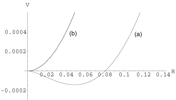
FIG. 1.: The effective potential of SU(2) QCD in the pure magnetic background. Here (a) is the effective potential and (b) is the classical potential.

IV Electric Background

To make sure that our infra-red regularization is indeed the correct one it is necessary to have an independent confirmation of the above result. To do this it is instructive to calculate the effective action with a pure electric background first.

So let us consider the general case where the background field strengh $\hat{F}_{\mu\nu}$ contains both electric and magnetic components. In this case we have

$$\hat{F}_{\mu\nu}=G_{\mu\nu}\hat{n},~{}~{}G_{\mu\nu}=F_{\mu\nu}+H_{\mu\nu},$$ (54)

and the functional determinants of the gluon and the ghost loops are generalized to

$${\rm Det}^{-\frac{1}{2}}K_{\mu\nu}^{ab}\simeq{\rm Det}^{-\frac{1}{2}}[-g_{\mu\nu}({\hat{D}}{\hat{D}})^{ab}-2gG_{\mu\nu}\epsilon^{abc}n^{c}],$$ (55)

$${\rm Det}M_{FP}={\rm Det}[-(\hat{D}\hat{D})^{ab}],$$ (56)

where now ${\hat{D}}_{\mu}$ is defined with an arbitrary background field ${\hat{A}}_{\mu}$. Using the relation

$$G_{\mu\alpha}G_{\alpha\beta}G_{\beta\nu}=-\displaystyle\frac{1}{2}G^{2}G_{\mu\nu}-\displaystyle\frac{1}{2}(G\tilde{G}){\tilde{G}}_{\mu\nu}~{}~{}~{}~{}({\tilde{G}}_{\mu\nu}=\displaystyle\frac{1}{2}{\epsilon}_{\mu\nu\rho\sigma}G_{\rho\sigma}),$$ (57)

one can simplify the functional determinants of the gluon and the quark loops as follows,

$$\ln{\rm Det}^{-\frac{1}{2}}[(-g_{\mu\nu}(\hat{D}\hat{D})^{ab}-2gG_{\mu\nu}\epsilon^{abc}n^{c}]=$$ (58)

$$\ln{\rm Det}[(-\tilde{D}^{2}+2a)(-\tilde{D}^{2}-2a)(-\tilde{D}^{2}-2ib)(-\tilde{D}^{2}+2ib)],$$ (59)

$$\ln{\rm Det}M_{FP}=2\ln{\rm Det}(-\tilde{D}^{2}),$$ (60)

where

$$a=\displaystyle\frac{g}{2}\sqrt{\sqrt{G^{4}+(G\tilde{G})^{2}}+G^{2}},\,\,\,\,b=\displaystyle\frac{g}{2}\sqrt{\sqrt{G^{4}+(G\tilde{G})^{2}}-G^{2}},$$ (61)

and now $\tilde{D}_{\mu}$ is defined with an arbitrary background $A_{\mu}+{\tilde{C}}_{\mu}$,

$$\tilde{D}_{\mu}=\partial+ig(A_{\mu}+{\tilde{C}}_{\mu}).$$ (62)

So for a pure electric background (i.e., for $a=0$) we have

$$\Delta{\cal L}=\displaystyle\frac{1}{16\pi^{2}}\int_{0}^{\infty}\displaystyle\frac{dt}{t^{2-\epsilon}}\displaystyle\frac{b}{\sin(bt)}[\exp(2ibt)+\exp(-2ibt)].$$ (63)

Notice that (unlike the pure magnetic background) the integrand of the above integral has poles on the real axis, so that we must specify the contour of the integral. Here the causality requires the contour to pass above the real axis.

There are different ways to evaluate the integral, but a simple and nice way of doing this follows from the observation that in the imaginary time (i.e., in the Minkowski time) the role of the electric and magnetic fields are reversed. So with the Wick rotation of the proper time $t$ to the imaginary time $it$, the above integral acquires the same form as (20). Indeed with the Wick rotation (39) becomes

$$\Delta{\cal L}\longrightarrow-\displaystyle\frac{1}{16\pi^{2}}i^{\epsilon}\int_{0}^{\infty}\displaystyle\frac{dt}{t^{2-\epsilon}}\displaystyle\frac{b}{\sinh(bt)}[\exp(-2bt)+\exp(2bt)].$$ (64)

From this we obtain

$$\Delta{{\cal L}}=-\displaystyle\frac{11b^{2}}{48\pi^{2}}(\displaystyle\frac{1}{\epsilon}-\gamma)+\displaystyle\frac{11b^{2}}{48\pi^{2}}(\ln\displaystyle\frac{b}{\mu^{2}}-c_{g})-i\displaystyle\frac{11b^{2}}{96\pi},$$ (65)

$$c_{g}=1-\ln 2-\displaystyle\frac{24}{11}\zeta^{\prime}(-1,\frac{3}{2})=0.94556....$$ (66)

So with the modified minimal subtraction we have (with the pure electric background)

$${\cal L}_{g}=\displaystyle\frac{b^{2}}{2g^{2}}+\displaystyle\frac{11b^{2}}{48\pi^{2}}(\ln\displaystyle\frac{b}{\mu^{2}}-c_{g})-i\displaystyle\frac{11b^{2}}{96\pi}.$$ (67)

It must be emphasized that in evaluating the above integral the same infra-red regularization is applied as in the pure magnetic background. With the pure electric background the eigenfunctions of Det K in the long distance region (i.e., for $k^{2}<b$) become anti-causal and thus unphysical, just like the eigenfunctions under the pure magnetic background become tachyonic and unphysical in the infra-red region (i.e., for $k^{2}<gH/\sqrt{2})$. So we must again exclude these unphysical modes to evaluate the above integral.

The contrast between the effective actions (22) and (42) is remarkable. First, (42) has no local minimum. This implies that the electric background does not generate a condensation. Secondly, (42) has an imaginary part

$$Im\thinspace{\cal L}_{g}=-\displaystyle\frac{11b^{2}}{96\pi}.$$ (68)

This implies that the electric background is unstable. But perhaps a more important point here is that the imaginary part is negative. This means that the electric background generates the pair annihilation, rather than the pair creation, of the gluons. This is because the negative imaginary part can be interpreted as the negative probability of the pair creation. This implies that the gluons in QCD, unlike the electrons in QED, tend to annihilate among themselves in the color electric field. This is really remarkable because this is precisely what one needs to explain the asymptotic freedom. Remember that the asymptotic freedom comes from the anti-screening effect, but for this anti-screening one needs the pair annihilation of gluons in the color electric flux. This means that our result is not only consistent with the asymptotic freedom, but actually explains why one must have the asymptotic freedom in QCD.

With this we can now make an independent confirmation of our effective actions (22) and (42). To do this first notice that the imaginary part (32) of the Savvidy-Nielsen-Olesen action as well as ours (22) and (42) are quadratic in the background fields. In our notation (38) this means that the imaginary part of the one loop effective action is second order in the coupling constant $g$. So one can find the correct imaginary part of the effective action perturbatively, just by calculating the effective action up to the second order in the coupling constant in the perturbative expansion. Now, a remarkable point is that by doing this one can reproduce our results [15],

$$Im\thinspace\Delta{\cal L}_{g}=\left\{{~{}~{}~{}~{}0~{}~{}~{}~{}~{}~{}~{}~{}~{}~{}~{}~{}~{}~{}b=0~{}~{}\atop-\displaystyle\frac{11b^{2}}{96\pi}~{}~{}~{}~{}~{}~{}~{}~{}~{}~{}~{}a=0~{}.}\right.$$ (69)

This confirms that our infra-red regularization is indeed correct. More importantly this confirms that we do have the desired dynamical symmetry breaking and the magnetic condensation in QCD. In the following we will provide a third independent argument which supports our results.

An important point to observe here is that the effective actions (22) and (42) are actually the mirror image of each other. To see this notice that we can obtain (42) from (22) simply by replacing $a=gH/\sqrt{2}$ with $-ib$, and similarly (22) from (42) by replacing $b$ with $ia=igH/\sqrt{2}$. This is the first indication that there exists a fundamental symmetry which we call the duality, in the effective action of QCD. We will discuss this duality in detail in the following.

The quark loop makes an extra contribution to the effective action. As we will see in the following we find for the massless quarks,

$$\Delta{\cal L}_{q} = -\displaystyle\frac{b^{2}}{48\pi^{2}}N_{f}(\ln\displaystyle\frac{b}{\mu^{2}}-c_{q})+i\displaystyle\frac{b^{2}}{96\pi},$$ (70)

$$c_{q} = \gamma+\ln(2\pi)+\displaystyle\frac{6}{\pi^{2}}\sum_{n=1}^{\infty}\displaystyle\frac{1}{n^{2}}\ln n.$$ (71)

So, together with (42), we obtain the following effective action

$${\cal L}_{eff}=\displaystyle\frac{b^{2}}{2g^{2}}+\displaystyle\frac{11-N_{f}}{48\pi^{2}}b^{2}(\ln\displaystyle\frac{b}{\mu^{2}}-c_{t}),$$ (72)

$$c_{t}=\displaystyle\frac{11}{11-N_{f}}c_{g}-\displaystyle\frac{1}{11-N_{f}}c_{q},$$ (73)

which is shown in Fig.2.

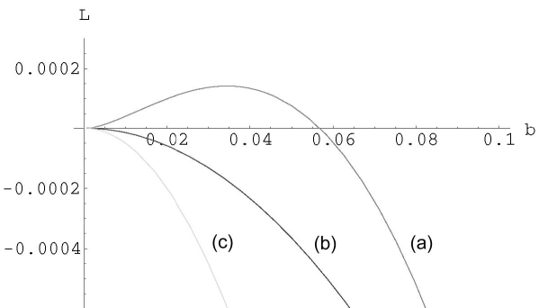
FIG. 2.: The effective action of SU(2) QCD in the pure electrical background. Here (a) is the real (dispersive) part of the effective action, (b) is the imaginary (absorptive) part of the effective action, and (c) is the classical action.

V Vacuum Stability

So far we have established the monopole condensation as a dynamical symmetry breaking. But this by itself does not allow us to claim that the monopole condensation provides the true physical vacuum. To show that the monopole condensation is indeed the unique vacuum of QCD, one must calculate the effective action with an arbitrary background of the restricted potential ${\hat{A}}_{\mu}$ and show that indeed the monopole condensation provides the true stable minimum of the effective potential.

For a general background with arbitrary $a$ and $b$, the contribution of the gluon and ghost loops corresponding to the functional determinant (37) is given by

$$\Delta{\cal L}_{g}=\displaystyle\frac{1}{16\pi^{2}}\int_{0}^{\infty}\displaystyle\frac{dt}{t^{3-\epsilon}}\displaystyle\frac{abt^{2}}{\sinh(at)\sin(bt)}$$ (74)

$$\times[\exp(-2at)+\exp(2at)+\exp(2ibt)+\exp(-2ibt)-2]$$ (75)

$$=\Delta{\cal L}_{1}+\Delta{\cal L}_{2}+\Delta{\cal L}_{3},$$ (76)

where

$$\Delta{\cal L}_{1}=\displaystyle\frac{1}{16\pi^{2}}\int_{0}^{\infty}\displaystyle\frac{dt}{t^{3-\epsilon}}\displaystyle\frac{abt^{2}}{\sinh(at)\sin(bt)}[\exp(-2at)+\exp(2at)],$$ (77)

$$\Delta{\cal L}_{2}=\displaystyle\frac{1}{16\pi^{2}}\int_{0}^{\infty}\displaystyle\frac{dt}{t^{3-\epsilon}}\displaystyle\frac{abt^{2}}{\sinh(at)\sin(bt)}[\exp(2ibt)+\exp(-2ibt)],$$ (78)

$$\Delta{\cal L}_{3}=-\displaystyle\frac{1}{8\pi^{2}}\int_{0}^{\infty}\displaystyle\frac{dt}{t^{3-\epsilon}}\displaystyle\frac{abt^{2}}{\sinh(at)\sin(bt)}.$$ (79)

Notice that $\Delta{\cal L}_{1}+\Delta{\cal L}_{2}$ describes the contribution of Det K of the gluon loop, but $\Delta{\cal L}_{3}$ describes the contribution of Det M of the ghost loop. Here again one should keep in mind that the contour of the integral should pass above the $t$-axis to preserve the causality.

The integral expression (47) of the effective action has been known for some time [13], but the actual integration of it is not easy to perform. Indeed, as far as we understand, the integration has not been completed satisfactorily. In the following we will perform the integral, and present a compact expression of the effective action. To carry out the integral we need to re-express the integrand in such a way that we can do the integral analytically. For this purpose we introduce the following identity [17],

$$\displaystyle\frac{xy}{\sinh(x)\sin(y)} = 1-\displaystyle\frac{x^{2}-y^{2}}{6}-\displaystyle\frac{2}{\pi}x^{3}y\sum_{n=1}^{\infty}\displaystyle\frac{(-1)^{n}}{n}\displaystyle\frac{{\rm csch}(\displaystyle\frac{n\pi y}{x})}{x^{2}+n^{2}\pi^{2}}$$ (80)

$$+ \displaystyle\frac{2}{\pi}xy^{3}\sum_{n=1}^{\infty}\displaystyle\frac{(-1)^{n}}{n}\displaystyle\frac{{\rm csch}(\displaystyle\frac{n\pi x}{y})}{y^{2}-n^{2}\pi^{2}}.$$ (81)

The identity, which we can establish using one of the Ramanujian’s identities[18], has played an important role in the calculation of the effective action of the scalar QED. Here again in QCD the same identity plays the crucial role in evaluating the effective action.

Now we can calculate $\Delta{\cal L}_{1},~{}\Delta{\cal L}_{2}$, and $\Delta{\cal L}_{3}$ separately with the help of our identity. Indeed using the identity (49) we obtain the following expression for $\Delta{\cal L}_{1}$,

$$\Delta{\cal L}_{1}=I_{1}(0,2a)+I_{1}(0,-2a)+I_{2}(0,2a)+I_{2}(0,-2a)+I_{3}(0,2a)+I_{3}(0,-2a),$$ (82)

where

$$I_{1}(\epsilon,\lambda) = \displaystyle\frac{1}{16\pi^{2}}\int_{0}^{\infty}t^{\epsilon-3}\Big{(}1-\displaystyle\frac{a^{2}-b^{2}}{6}t^{2}\Big{)}e^{-\lambda t}dt$$ (83)

$$= \displaystyle\frac{1}{16\pi^{2}}\lambda^{-\epsilon}\Big{[}\displaystyle\frac{\lambda^{2}}{2}(1+\displaystyle\frac{3}{2}\epsilon)-\displaystyle\frac{a^{2}-b^{2}}{6}\Big{]}\Gamma(\epsilon),$$ (84)

$$I_{2}(\epsilon,\lambda) = -\displaystyle\frac{ab}{8\pi^{2}}\sum_{n=1}^{\infty}\displaystyle\frac{(-1)^{n}}{n}{\rm csch}(\displaystyle\frac{n\pi b}{a})\int_{0}^{\infty}t^{\epsilon+1}\displaystyle\frac{e^{-\lambda t}}{t^{2}+(\displaystyle\frac{n\pi}{a})^{2}}dt$$ (85)

$$= \displaystyle\frac{ab}{8\pi^{3}}\sum_{n=1}^{\infty}\displaystyle\frac{(-1)^{n}}{n}{\rm csch}(\displaystyle\frac{n\pi b}{a})[{\rm ci}(\displaystyle\frac{n\pi\lambda}{a})\cos(\displaystyle\frac{n\pi\lambda}{a})+{\rm si}(\displaystyle\frac{n\pi\lambda}{a})\sin(\displaystyle\frac{n\pi\lambda}{a})],$$ (86)

$$I_{3}(\epsilon,\lambda) = \displaystyle\frac{ab}{8\pi^{2}}\sum_{n=1}^{\infty}\displaystyle\frac{(-1)^{n}}{n}{\rm csch}(\displaystyle\frac{n\pi a}{b})\int_{0}^{\infty}t^{\epsilon+1}\displaystyle\frac{e^{-\lambda t}}{t^{2}-(\displaystyle\frac{n\pi}{b})^{2}}dt$$ (87)

$$= -\displaystyle\frac{ab}{16\pi^{3}}\sum_{n=1}^{\infty}\displaystyle\frac{(-1)^{n}}{n}{\rm csch}(\displaystyle\frac{n\pi a}{b})[{\rm Ei}(-\displaystyle\frac{n\pi\lambda}{b})\exp(\displaystyle\frac{n\pi\lambda}{a})+{\rm Ei}(\displaystyle\frac{n\pi\lambda}{b})\exp(-\displaystyle\frac{n\pi\lambda}{a})].$$ (88)

Notice that here ci($x$) and si($x$) are the cosine and sine integral functions, and Ei($-x$) is the exponential integral function [19],

$${\rm ci}(x) = -\int_{x}^{\infty}\displaystyle\frac{\cos(t)}{t}dt$$ (89)

$$= \gamma+\ln x+\sum_{n=1}^{\infty}\displaystyle\frac{(-1)^{n}x^{2n}}{(2n)!2n},~{}~{}~{}~{}~{}~{}~{}~{}~{}~{}({\rm Re}~{}x>0)$$ (90)

$${\rm si}(x) = -\int_{x}^{\infty}\displaystyle\frac{\sin(t)}{t}dt$$ (91)

$$= -\displaystyle\frac{\pi}{2}-\sum_{n=1}^{\infty}\displaystyle\frac{(-1)^{n}x^{2n-1}}{(2n-1)!(2n-1)},~{}~{}~{}~{}~{}({\rm Re}~{}x>0)$$ (92)

$${\rm Ei}(-x) = -\int_{x}^{\infty}\displaystyle\frac{e^{-t}}{t}dt$$ (93)

$$= \gamma+\ln x+\sum_{n=1}^{\infty}\displaystyle\frac{(-1)^{n}x^{n}}{(n)!n}.~{}~{}~{}~{}~{}~{}~{}~{}~{}~{}~{}~{}({\rm Re}~{}x>0)$$ (94)

With these we find

$$\Delta{\cal L}_{1} = \displaystyle\frac{11a^{2}+b^{2}}{48\pi^{2}}(\displaystyle\frac{1}{\epsilon}-\gamma)+\displaystyle\frac{3a^{2}}{8\pi^{2}}-\displaystyle\frac{11a^{2}+b^{2}}{48\pi^{2}}\ln(\displaystyle\frac{2a}{\mu^{2}})$$ (95)

$$+ \displaystyle\frac{ab}{4\pi^{3}}\sum_{n=1}^{\infty}\displaystyle\frac{(-1)^{n}}{n}{\rm csch}(\displaystyle\frac{n\pi b}{a}){\rm ci}(2n\pi)$$ (96)

$$- \displaystyle\frac{ab}{8\pi^{3}}\sum_{n=1}^{\infty}\displaystyle\frac{(-1)^{n}}{n}{\rm csch}(\displaystyle\frac{n\pi a}{b})\Big{[}{\rm Ei}(-\displaystyle\frac{2n\pi a}{b})\exp(\frac{2n\pi a}{b})$$ (97)

$$+ \bar{{\rm Ei}}(\displaystyle\frac{2n\pi a}{b})\exp(-\frac{2n\pi a}{b})\Big{]}+i\displaystyle\frac{a^{2}}{96\pi}$$ (98)

$$- i\displaystyle\frac{ab}{8\pi^{2}}\sum_{n=1}^{\infty}\displaystyle\frac{(-1)^{n}}{n}\Big{[}{\rm csch}(\displaystyle\frac{n\pi b}{a})+{\rm csch}(\displaystyle\frac{n\pi a}{b})\exp(-\frac{2n\pi a}{b})\Big{]},$$ (99)

where $\bar{\rm Ei}(x)$ is ${\rm Re~{}Ei}(x)$. To obtain the above result notice that, for $\lambda=-2a$, a naive integration of (51) gives an infra-red divergence. So one must perform the integral with a positive $\lambda$ first, and then make an analytic continuation to $\lambda=-2a$. In this analytic continuation one must keep in mind two points. First, the analytic continuation should preserve the causality. This means that we must select the correct (i.e., physical) branch in the analytic continuation of ci($x$), si($x$), and Ei($-x$) to the negative real axis. Secondly, the continuation must be done in such a way that the unphysical modes should have no contribution. This requires that the imaginary component of $\Delta{\cal L}_{1}$ should reproduce the previous result (21) in the pure magnetic background. With these precautions we obtain the above result.

Now it is simple to evaluate $\Delta{\cal L}_{2}$, because it can be put into the same form as $\Delta{\cal L}_{1}$ with a Wick rotation of $t$ to $it$. Indeed we have (after the Wick rotation)

$$\Delta{\cal L}_{2}=-\displaystyle\frac{1}{16\pi^{2}}i^{\epsilon}\int_{0}^{\infty}\displaystyle\frac{dt}{t^{3-\epsilon}}\displaystyle\frac{abt^{2}}{\sinh(bt)\sin(at)}[\exp(-2bt)+\exp(2bt)].$$ (100)

But an important point to notice here is that with the Wick rotation the contour of the above integral should now pass below the $t$-axis. With this observation we obtain

$$\Delta{\cal L}_{2}= - \displaystyle\frac{11b^{2}+a^{2}}{48\pi^{2}}(\displaystyle\frac{1}{\epsilon}-\gamma)-\displaystyle\frac{3b^{2}}{8\pi^{2}}+\displaystyle\frac{11b^{2}+a^{2}}{48\pi^{2}}\ln(\displaystyle\frac{2b}{\mu^{2}})$$ (101)

$$- \displaystyle\frac{ab}{4\pi^{3}}\sum_{n=1}^{\infty}\displaystyle\frac{(-1)^{n}}{n}{\rm csch}(\displaystyle\frac{n\pi a}{b}){\rm ci}(2n\pi)$$ (102)

$$+ \displaystyle\frac{ab}{8\pi^{3}}\sum_{n=1}^{\infty}\displaystyle\frac{(-1)^{n}}{n}{\rm csch}(\displaystyle\frac{n\pi b}{a})\Big{[}{\rm Ei}(-\displaystyle\frac{2n\pi b}{a})\exp(\frac{2n\pi b}{a})$$ (103)

$$+ \bar{{\rm Ei}}(\displaystyle\frac{2n\pi b}{a})\exp(-\frac{2n\pi b}{a})\Big{]}-i\displaystyle\frac{11b^{2}}{96\pi}$$ (104)

$$+ i\displaystyle\frac{ab}{8\pi^{2}}\sum_{n=1}^{\infty}\displaystyle\frac{(-1)^{n}}{n}\Big{[}{\rm csch}(\displaystyle\frac{n\pi a}{b})-{\rm csch}(\displaystyle\frac{n\pi b}{a})\exp(-\frac{2n\pi b}{a})\Big{]}.$$ (105)

Again we emphasize that the above Wick rotation prescription automatically and naturally guarantees that we have the same infra-red regularization in the evaluation of $\Delta{\cal L}_{1}$ and $\Delta{\cal L}_{2}$. Indeed we can easily confirm that $\Delta{\cal L}_{2}$ reproduces the previous result (41) in the pure electric background (i.e., in the limit $a$ goes to zero), as it should.

Finally it is straightforward to calculate $\Delta{\cal L}_{3}$, because it has no infra-red divergence. We find

$$\Delta{\cal L}_{3} = -\displaystyle\frac{1}{8\pi^{2}}\int_{0}^{\infty}\displaystyle\frac{dt}{t^{3-\epsilon}}\displaystyle\frac{abt^{2}}{\sinh(at)\sin(bt)}$$ (106)

$$= -2\Big{(}I_{1}(0,0)+I_{2}(0,0)+I_{3}(0,0)\Big{)}.$$ (107)

From this we have

$$\Delta{\cal L}_{3}=\displaystyle\frac{a^{2}-b^{2}}{48\pi^{2}}(\displaystyle\frac{1}{\epsilon}-\gamma)-\displaystyle\frac{ab}{4\pi^{3}}\sum_{n=1}^{\infty}\displaystyle\frac{(-1)^{n}}{n}\Big{[}{\rm csch}(\displaystyle\frac{n\pi b}{a})\Big{(}\ln(\displaystyle\frac{n\pi\mu^{2}}{a})+\gamma\Big{)}$$ (108)

$$-{\rm csch}(\displaystyle\frac{n\pi a}{b})\Big{(}\ln(\displaystyle\frac{n\pi\mu^{2}}{b})+\gamma\Big{)}\Big{]}+i\displaystyle\frac{ab}{8\pi^{3}}\sum_{n=1}^{\infty}\displaystyle\frac{(-1)^{n}}{n}{\rm csch}(\displaystyle\frac{n\pi a}{b}).$$ (109)

To obtain the above result we have used the following identity [17],

$$\displaystyle\frac{12}{\pi}ab\sum_{n=1}^{\infty}\displaystyle\frac{(-1)^{n}}{n}\Big{[}{\rm csch}(\displaystyle\frac{n\pi b}{a})-{\rm csch}(\displaystyle\frac{n\pi a}{b})\Big{]}=b^{2}-a^{2}.$$ (110)

In evaluating the integrals it should be stressed again that one must be very careful to implement a proper infra-red regularization. In particular, one has to make sure that the above result reproduces the results of the previous sections for the pure magnetic and the pure electric backgrounds.

With the above results we finally obtain (after the modified minimal subtraction)

$$\Delta{\cal L}_{g} = \Delta{\cal L}_{1}+\Delta{\cal L}_{2}+\Delta{\cal L}_{3}$$ (111)

$$= \displaystyle\frac{3a^{2}-3b^{2}}{8\pi^{3}}-\displaystyle\frac{11a^{2}+b^{2}}{48\pi^{2}}\ln(\displaystyle\frac{2a}{\mu^{2}})+\displaystyle\frac{11b^{2}+a^{2}}{48\pi^{2}}\ln(\displaystyle\frac{2b}{\mu^{2}})$$ (112)

$$+ \displaystyle\frac{ab}{4\pi^{3}}\sum_{n=1}^{\infty}\displaystyle\frac{(-1)^{n}}{n}\Big{(}{\rm csch}(\displaystyle\frac{n\pi b}{a})-{\rm csch}(\displaystyle\frac{n\pi a}{b})\Big{)}({\rm ci}(2n\pi)-\gamma)$$ (113)

$$+ \displaystyle\frac{ab}{8\pi^{3}}\sum_{n=1}^{\infty}\displaystyle\frac{(-1)^{n}}{n}\Big{[}{\rm csch}(\displaystyle\frac{n\pi b}{a})\Big{(}\exp(\frac{2n\pi b}{a}){\rm Ei}(-\displaystyle\frac{2n\pi b}{a})$$ (114)

$$+ \exp(-\frac{2n\pi b}{a})\bar{{\rm Ei}}(\displaystyle\frac{2n\pi b}{a})\Big{)}-{\rm csch}(\displaystyle\frac{n\pi a}{b})\Big{(}\exp(\frac{2n\pi a}{b}){\rm Ei}(-\displaystyle\frac{2n\pi a}{b})$$ (115)

$$+ \exp(-\frac{2n\pi a}{b})\bar{{\rm Ei}}(\displaystyle\frac{2n\pi a}{b})\Big{)}\Big{]}$$ (116)

$$- \displaystyle\frac{ab}{4\pi^{3}}\sum_{n=1}^{\infty}\displaystyle\frac{(-1)^{n}}{n}\Big{(}{\rm csch}(\displaystyle\frac{n\pi b}{a})\ln(\displaystyle\frac{n\pi\mu^{2}}{a})-{\rm csch}(\displaystyle\frac{n\pi a}{b})\ln(\displaystyle\frac{n\pi\mu^{2}}{b})\Big{)}$$ (117)

$$- i\displaystyle\frac{a^{2}+11b^{2}}{96\pi}-i\displaystyle\frac{ab}{8\pi^{2}}\sum_{n=1}^{\infty}\displaystyle\frac{(-1)^{n}}{n}\Big{(}{\rm csch}(\displaystyle\frac{n\pi b}{a})\exp(-\frac{2n\pi b}{a})$$ (118)

$$+ {\rm csch}(\displaystyle\frac{n\pi a}{b})\exp(-\frac{2n\pi a}{b})\Big{)}+i\displaystyle\frac{ab}{8\pi^{2}}\sum_{n=1}^{\infty}\displaystyle\frac{(-1)^{n}}{n}{\rm csch}(\displaystyle\frac{n\pi a}{b}).$$ (119)

Notice again that here we have used our identity (58) to obtain the above result. The result is summarized in Fig.3 and Fig.4, where we have plotted the gluon contribution of the dispersive and absorbtive parts of the effective action.

An important point here is that the effective action acquires the following imaginary component,

$$Im\Delta{\cal L}_{g}= - \displaystyle\frac{a^{2}+11b^{2}}{96\pi}-\displaystyle\frac{ab}{8\pi^{2}}\sum_{n=1}^{\infty}\displaystyle\frac{(-1)^{n}}{n}\Big{(}{\rm csch}(\displaystyle\frac{n\pi b}{a})\exp(-\frac{2n\pi b}{a})$$ (120)

$$+ {\rm csch}(\displaystyle\frac{n\pi a}{b})\exp(-\frac{2n\pi a}{b})\Big{)}+\displaystyle\frac{ab}{8\pi^{2}}\sum_{n=1}^{\infty}\displaystyle\frac{(-1)^{n}}{n}{\rm csch}(\displaystyle\frac{n\pi a}{b}).$$ (121)

We can confirm that this expression reproduces the previous results. Indeed we find

$$Im\thinspace\Delta{\cal L}_{1}=\left\{{~{}~{}~{}~{}0~{}~{}~{}~{}~{}~{}~{}~{}~{}~{}~{}~{}~{}~{}b=0~{}~{}\atop~{}~{}~{}\displaystyle\frac{b^{2}}{96\pi}~{}~{}~{}~{}~{}~{}~{}~{}~{}~{}~{}a=0~{},}\right.$$ (122)

$$Im\Delta{\cal L}_{2}=\left\{{~{}~{}~{}~{}0~{}~{}~{}~{}~{}~{}~{}~{}~{}~{}~{}~{}~{}~{}b=0~{}~{}\atop-\displaystyle\frac{11b^{2}}{96\pi}~{}~{}~{}~{}~{}~{}~{}~{}~{}~{}a=0~{},}\right.$$ (123)

$$Im\Delta{\cal L}_{3}=\left\{{~{}~{}~{}~{}0~{}~{}~{}~{}~{}~{}~{}~{}~{}~{}~{}~{}~{}~{}b=0~{}~{}\atop-\displaystyle\frac{b^{2}}{96\pi}~{}~{}~{}~{}~{}~{}~{}~{}~{}~{}~{}a=0~{},}\right.$$ (124)

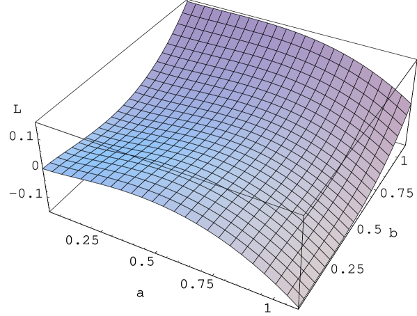
FIG. 3.: The real (dispersive) part of the gluon contribution to the effective action of SU(2) QCD.

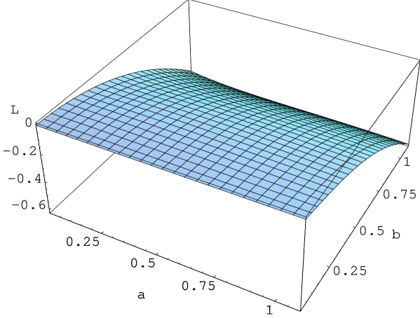
FIG. 4.: The imaginary (absorptive) part of the gluon contribution to the effective action of SU(2) QCD.

so that

$$Im\Delta{\cal L}_{g}=\left\{{~{}~{}~{}~{}0~{}~{}~{}~{}~{}~{}~{}~{}~{}~{}~{}~{}~{}~{}~{}b=0~{}~{}\atop-\displaystyle\frac{11b^{2}}{96\pi}~{}~{}~{}~{}~{}~{}~{}~{}~{}~{}~{}a=0~{}.}\right.$$ (125)

What is really remarkable about the above result is the unilateral emergence of the imaginary part with $b\neq 0$. This immediately tells that the color electric background generates an instability to the effective action. Only when the background becomes pure magnetic the imaginary part disappears completely. This automatically proves that the monopole condensation is indeed the unique and stable vacuum of QCD, at least in one loop approximation.

Observe that the imaginary part of the effective action becomes negative in general. This assures again that the electric background makes the pair annihilation for the gluons, but not the pair creation. In contrast, as we will see in the following, the electric background makes the pair creation for the quarks. This is a very important observation, because this tells that the gluon pairs behave differently from the quark pairs in the color electric field. In particular the valence gluons are not likely to form the glueball bound states. This explains the experimental fact that there are so few (if at all) candidates of glueball bound states, while we have towers of hadronic bound states made of quarks.

VI Quark Contribution

Obviously one can not neglect the quarks in QCD. Let us consider the Lagrangian involving the $SU(2)$ quarks in the fundamental representation

$${\cal L}_{q}=\bar{\Psi}(i\gamma^{\mu}D_{\mu}-m_{q})\Psi,$$ (126)

$$D_{\mu}=\partial_{\mu}+\displaystyle\frac{g}{2i}{\vec{\sigma}}\cdot{\vec{A}}_{\mu},$$ (127)

where $m_{q}$ is the mass of the quarks. One can express the quark contribution to the effective action in one loop approximation by

$$\Delta{\cal L}_{q}=-\displaystyle\frac{ab}{16\pi^{2}}N_{f}\int_{0}^{\infty}\displaystyle\frac{dt}{t^{1-\epsilon}}\coth(at)\cot(bt)\exp(-m_{q}^{2}t),$$ (128)

Notice that formally this is very much like the well-known expression of the one loop contribution of electron to the effective action in QED [16, 17]. This is because at one loop level only the interaction of the quarks with the restricted potential contributes to the effective action.

We can evaluate the above integral exactly the same way as we calculate the electron loop contribution in QED [17]. Using the following Sitaramachandrarao’s identity [17, 18],

$$xy\coth(x)\cot(y) = 1+\displaystyle\frac{x^{2}-y^{2}}{3}-\displaystyle\frac{2}{\pi}x^{3}y\sum_{n=1}^{\infty}\displaystyle\frac{1}{n}\displaystyle\frac{{\rm csch}(\displaystyle\frac{n\pi y}{x})}{x^{2}+n^{2}\pi^{2}}$$ (129)

$$+ \displaystyle\frac{2}{\pi}xy^{3}\sum_{n=1}^{\infty}\displaystyle\frac{1}{n}\displaystyle\frac{{\rm csch}(\displaystyle\frac{n\pi x}{y})}{y^{2}-n^{2}\pi^{2}},$$ (130)

we obtain (with the modified minimal subtraction),

$$\Delta{\cal L}_{q} = \displaystyle\frac{a^{2}-b^{2}}{48\pi^{2}}\ln\displaystyle\frac{m_{q}^{2}}{\mu^{2}}$$ (131)

$$- \displaystyle\frac{ab}{8\pi^{3}}N_{f}\sum_{n=1}^{\infty}\displaystyle\frac{1}{n}{\rm coth}(\displaystyle\frac{n\pi b}{a})\Big{(}{\rm ci}(\displaystyle\frac{2n\pi m_{q}^{2}}{a})\cos(\displaystyle\frac{2n\pi m_{q}^{2}}{a})+{\rm si}(\displaystyle\frac{2n\pi m_{q}^{2}}{a})\sin(\displaystyle\frac{2n\pi m_{q}^{2}}{a})\Big{)}$$ (132)

$$+ \displaystyle\frac{ab}{16\pi^{3}}N_{f}\sum_{n=1}^{\infty}\displaystyle\frac{1}{n}{\rm coth}(\displaystyle\frac{n\pi a}{b})\Big{(}{\rm Ei}(-\displaystyle\frac{2n\pi m_{q}^{2}}{b})\exp(\displaystyle\frac{2n\pi m_{q}^{2}}{b})$$ (133)

$$+ {\rm Ei}(\displaystyle\frac{2n\pi m_{q}^{2}}{b})\exp(-\displaystyle\frac{2n\pi m_{q}^{2}}{b})\Big{)}.$$ (134)

Notice that the above effective action of the quark loop also develops an imaginary part when $b\neq 0$,

$$Im\thinspace\Delta{\cal L}_{q}=\displaystyle\frac{ab}{16\pi^{2}}N_{f}\sum_{n=1}^{\infty}\displaystyle\frac{1}{n}{\rm coth}(\displaystyle\frac{n\pi a}{b})\exp(-\displaystyle\frac{2n\pi m_{q}^{2}}{b}).$$ (135)

This is because the exponential integral Ei($-x$) in (66) develops an imaginary part after the analytic continuation from $x$ to $-x$. One can compare this with the imaginary part of the gluon loop (60). Remarkably the signature of the imaginary part of the quark loop is opposite to that of the gluon loop. This is due to the opposite statistics between the gluons and the quarks, which gives an overall minus sign for the quark loop in (64). This tells that the quarks should contribute a positive imaginary part to the effective action when $b\neq 0$, This means that, just like in QED, the electric flux of the quarks generates the pair creation and the color screening effect, rather than the pair annihilation and the color anti-screening effect. This allows the quarks to form the hadronic bound states.

Observe that in the pure magnetic and pure electric limits the above result reduces to

$$\Delta{\cal L}_{q}=\left\{{\displaystyle\frac{a^{2}}{48\pi^{2}}\ln\displaystyle\frac{m_{q}^{2}}{\mu^{2}}-\displaystyle\frac{a^{2}}{8\pi^{4}}N_{f}\sum_{n=1}^{\infty}\displaystyle\frac{1}{n^{2}}\Big{(}{\rm ci}(\displaystyle\frac{2n\pi m_{q}^{2}}{a})\cos(\displaystyle\frac{2n\pi m_{q}^{2}}{a})\Big{)}~{}~{}~{}~{}~{}~{}~{}~{}~{}~{}~{}~{}~{}~{}~{}~{}~{}~{}b=0,\atop-\displaystyle\frac{b^{2}}{48\pi^{2}}\ln\displaystyle\frac{m_{q}^{2}}{\mu^{2}}+\displaystyle\frac{b^{2}}{16\pi^{4}}N_{f}\sum_{n=1}^{\infty}\displaystyle\frac{1}{n^{2}}\Big{(}{\rm Ei}(-\displaystyle\frac{2n\pi m_{q}^{2}}{b})\exp(\displaystyle\frac{2n\pi m_{q}^{2}}{b})\Big{)}~{}~{}~{}~{}~{}~{}~{}~{}~{}~{}a=0.}\right.$$ (136)

The contribution of the quark loop to the effective action is plotted in Fig.5 and Fig.6 . In view of the experimental fact that $\Lambda_{\bar{MS}}\simeq 250$ Mev and $m_{q}\simeq 5$ Mev, we have assumed $m_{q}=0.02$ to obtain the figures.

Notice that in the massless limit we have[17]

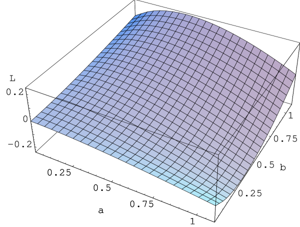
FIG. 5.: The real (dispersive) part of the quark contribution to the effective action of SU(2) QCD.

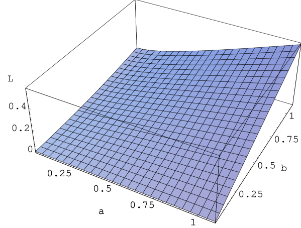
FIG. 6.: The imaginary (absorptive) part of the quark contribution to the effective action of SU(2) QCD.

$$\Delta{\cal L}_{q}\Big{|}_{m_{q}=0} \simeq \displaystyle\frac{N_{f}}{48\pi^{2}}\Big{[}a^{2}-b^{2}-\displaystyle\frac{6ab}{\pi}\sum_{n=1}^{\infty}\displaystyle\frac{1}{n}\Big{(}{\rm coth}(\displaystyle\frac{n\pi b}{a})-{\rm coth}(\displaystyle\frac{n\pi a}{b})\Big{)}\Big{]}\ln\Big{(}\displaystyle\frac{m_{q}}{\mu}\Big{)}^{2}$$ (137)

$$- \displaystyle\frac{ab}{8\pi^{3}}N_{f}\sum_{n=1}^{\infty}\displaystyle\frac{1}{n}\Big{[}{\rm coth}(\displaystyle\frac{n\pi b}{a})\Big{(}\ln(\displaystyle\frac{2n\pi\mu^{2}}{a})+\gamma\Big{)}-{\rm coth}(\displaystyle\frac{n\pi a}{b})\Big{(}\ln(\displaystyle\frac{2n\pi\mu^{2}}{b})+\gamma\Big{)}\Big{]}$$ (138)

$$+ i\displaystyle\frac{ab}{16\pi^{2}}N_{f}\sum_{n=1}^{\infty}\displaystyle\frac{1}{n}{\rm coth}(\displaystyle\frac{n\pi a}{b}),$$ (139)

so that, when $ab\neq 0$, the effective action from the quark loop (unlike the gluon loop) becomes divergent in the massless limit. This is because here the infra-red divergence comes from the zero modes which are physical, so that the infra-red divergence can not be removed.

One could separate the divergent part from the finite part in $\Delta{\cal L}_{q}$. We find

$$\Delta{\cal L}_{q}\Big{|}_{m_{q}=0}=\Delta{\cal L}_{\infty}+\Delta{\cal L}_{\rm fin},$$ (140)

where

$$\Delta{\cal L}_{\infty} \simeq \displaystyle\frac{N_{f}}{48\pi^{2}}\Big{[}a^{2}-b^{2}-\displaystyle\frac{6ab}{\pi}\sum_{n=1}^{\infty}\displaystyle\frac{1}{n}\Big{(}{\rm coth}(\displaystyle\frac{n\pi b}{a})-{\rm coth}(\displaystyle\frac{n\pi a}{b})\Big{)}\Big{]}\ln\Big{(}\displaystyle\frac{m_{q}}{\mu}\Big{)}^{2}$$ (141)

$$+ \displaystyle\frac{ab}{16\pi^{3}}N_{f}\sum_{n=1}^{\infty}\Big{(}{\rm coth}(\displaystyle\frac{n\pi b}{a})+{\rm coth}(\displaystyle\frac{n\pi a}{b})\Big{)}\ln\displaystyle\frac{a}{b}$$ (142)

$$+ i\displaystyle\frac{ab}{16\pi^{2}}N_{f}\sum_{n=1}^{\infty}\displaystyle\frac{1}{n}{\rm coth}(\displaystyle\frac{n\pi a}{b}),$$ (143)

$$\Delta{\cal L}_{\rm fin} = -\displaystyle\frac{ab}{16\pi^{2}}N_{f}\sum_{n=1}^{\infty}\displaystyle\frac{1}{n}\Big{(}{\rm coth}(\displaystyle\frac{n\pi b}{a})-{\rm coth}(\displaystyle\frac{n\pi a}{b})\Big{)}$$ (145)

$$\Big{(}2\gamma+\ln(\displaystyle\frac{2n\pi\mu^{2}}{a})+\ln(\displaystyle\frac{2n\pi\mu^{2}}{b})\Big{)}.$$

This tells that one has to keep $m_{q}$ finite in the evaluation of the effective action of QCD when $ab\neq 0$, to avoid the infra-red divergence of the quark loop.

But notice that, when $ab=0$, the logarithmic divergence in (69) disappears due to the following identity [17],

$$\displaystyle\frac{6ab}{\pi}\sum_{n=1}^{\infty}\displaystyle\frac{1}{n}\Big{(}{\rm coth}(\displaystyle\frac{n\pi b}{a})-{\rm coth}(\displaystyle\frac{n\pi a}{b})\Big{)}=a^{2}-b^{2}.$$ (146)

So in this case (i.e., when $ab=0$) $\Delta{\cal L}_{q}$ becomes finite even in the massless limit,

$$\Delta{\cal L}_{q}\Big{|}_{m_{q}=0}=\left\{{~{}\displaystyle\frac{a^{2}}{48\pi^{2}}N_{f}(\ln\displaystyle\frac{a}{\mu^{2}}-c_{q})~{}~{}~{}~{}~{}~{}~{}~{}~{}~{}~{}~{}~{}~{}~{}~{}~{}~{}~{}~{}~{}~{}~{}b=0\atop-\displaystyle\frac{b^{2}}{48\pi^{2}}N_{f}(\ln\displaystyle\frac{b}{\mu^{2}}-c_{q})+i\displaystyle\frac{b^{2}}{96\pi}~{}~{}~{}~{}~{}~{}~{}~{}~{}~{}~{}~{}a=0,}\right.$$ (147)

where

$$c_{q}=\gamma+\ln(2\pi)+\displaystyle\frac{6}{\pi^{2}}\sum_{n=1}^{\infty}\displaystyle\frac{1}{n^{2}}\ln n=2.98504...$$ (148)

Notice that we can also obtain the above result from (68) by making the massless limit of the quarks.

VII Effective Action and Duality

With the above analysis we can sum up the gluon and quark contributions and obtain the following final effective action of $SU(2)$ QCD,

$${\cal L}_{eff} = {\cal L}_{0}+\Delta{\cal L}_{g}+\Delta{\cal L}_{q}$$ (149)

$$= -\displaystyle\frac{a^{2}-b^{2}}{2g^{2}}+\displaystyle\frac{3a^{2}-3b^{2}}{8\pi^{3}}-\displaystyle\frac{11a^{2}+b^{2}}{48\pi^{2}}\ln(\displaystyle\frac{2a}{\mu^{2}})+\displaystyle\frac{11b^{2}+a^{2}}{48\pi^{2}}\ln(\displaystyle\frac{2b}{\mu^{2}})+\displaystyle\frac{a^{2}-b^{2}}{48\pi^{2}}\ln\displaystyle\frac{m_{q}^{2}}{\mu^{2}}$$ (150)

$$+ \displaystyle\frac{ab}{4\pi^{3}}\sum_{n=1}^{\infty}\displaystyle\frac{(-1)^{n}}{n}\Big{(}{\rm csch}(\displaystyle\frac{n\pi b}{a})-{\rm csch}(\displaystyle\frac{n\pi a}{b})\Big{)}({\rm ci}(2n\pi)-\gamma)$$ (151)

$$+ \displaystyle\frac{ab}{8\pi^{3}}\sum_{n=1}^{\infty}\displaystyle\frac{(-1)^{n}}{n}\Big{[}{\rm csch}(\displaystyle\frac{n\pi b}{a})\Big{(}\exp(\frac{2n\pi b}{a}){\rm Ei}(-\displaystyle\frac{2n\pi b}{a})+\exp(-\frac{2n\pi b}{a})\bar{{\rm Ei}}(\displaystyle\frac{2n\pi b}{a})\Big{)}$$ (152)

$$- {\rm csch}(\displaystyle\frac{n\pi a}{b})\Big{(}\exp(\frac{2n\pi a}{b}){\rm Ei}(-\displaystyle\frac{2n\pi a}{b})+\exp(-\frac{2n\pi a}{b})\bar{{\rm Ei}}(\displaystyle\frac{2n\pi a}{b})\Big{)}\Big{]}$$ (153)

$$- \displaystyle\frac{ab}{4\pi^{3}}\sum_{n=1}^{\infty}\displaystyle\frac{(-1)^{n}}{n}\Big{(}{\rm csch}(\displaystyle\frac{n\pi b}{a})\ln(\displaystyle\frac{n\pi\mu^{2}}{a})-{\rm csch}(\displaystyle\frac{n\pi a}{b})\ln(\displaystyle\frac{n\pi\mu^{2}}{b})\Big{)}$$ (154)

$$+ \displaystyle\frac{ab}{8\pi^{3}}N_{f}\sum_{n=1}^{\infty}\displaystyle\frac{1}{n}{\rm coth}(\displaystyle\frac{n\pi b}{a})\Big{(}{\rm ci}(\displaystyle\frac{2n\pi m_{q}^{2}}{a})\cos(\displaystyle\frac{2n\pi m_{q}^{2}}{a})+{\rm si}(\displaystyle\frac{2n\pi m_{q}^{2}}{a})\sin(\displaystyle\frac{2n\pi m_{q}^{2}}{a})\Big{)}$$ (155)

$$+ \displaystyle\frac{ab}{16\pi^{3}}N_{f}\sum_{n=1}^{\infty}\displaystyle\frac{1}{n}{\rm coth}(\displaystyle\frac{n\pi a}{b})\Big{(}{\rm Ei}(-\displaystyle\frac{2n\pi m_{q}^{2}}{b})\exp(\displaystyle\frac{2n\pi m_{q}^{2}}{b})+{\rm Ei}(\displaystyle\frac{2n\pi m_{q}^{2}}{b})\exp(-\displaystyle\frac{2n\pi m_{q}^{2}}{b})\Big{)}$$ (156)

$$- i\displaystyle\frac{a^{2}+11b^{2}}{96\pi}-i\displaystyle\frac{ab}{8\pi^{2}}\sum_{n=1}^{\infty}\displaystyle\frac{(-1)^{n}}{n}\Big{(}{\rm csch}(\displaystyle\frac{n\pi b}{a})\exp(-\frac{2n\pi b}{a})$$ (157)

$$+ {\rm csch}(\displaystyle\frac{n\pi a}{b})\exp(-\frac{2n\pi a}{b})\Big{)}+i\displaystyle\frac{ab}{8\pi^{2}}\sum_{n=1}^{\infty}\displaystyle\frac{(-1)^{n}}{n}{\rm csch}(\displaystyle\frac{n\pi a}{b})$$ (158)

$$+ i\displaystyle\frac{ab}{16\pi^{2}}N_{f}\sum_{n=1}^{\infty}\displaystyle\frac{1}{n}{\rm coth}(\displaystyle\frac{n\pi a}{b})\exp(-\displaystyle\frac{2n\pi m_{q}^{2}}{b}).$$ (159)

From this we finally obtain Fig.7 and Fig.8, which describe the real and imaginary parts of the total effective action of $SU(2)$ QCD. Remember that we have assumed $\alpha_{s}=1,\,\mu=1,\,m_{q}=0.02,$ and $N_{f}=2$ to obtain the figures.

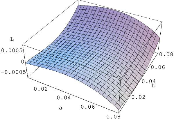
FIG. 7.: The real (dispersive) part of the effective action of SU(2) QCD.

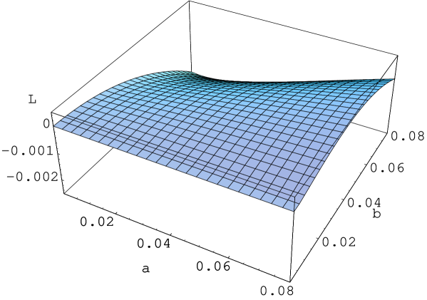
FIG. 8.: The imaginary (absorptive) part of the effective action of SU(2) QCD.

A truly remarkable feature of our effective action is that it is manifestly invariant under the dual transformation

$$a\rightarrow-ib,~{}~{}~{}~{}b\rightarrow ia.$$ (160)

In fact $\Delta{\cal L}_{g}$ and $\Delta{\cal L}_{q}$ independently can be shown to be invariant under the dual transformation. This tells that, as a function of $z=a+ib,$ the effective action of QCD is invariant under the reflection from $z$ to $-z$. To establish the duality in the effective action it is important to realize that the argument of the special functions ci($x$), si($x$), and Ei($-x$) changes the signature under the dual transformation. So the dual transformation automatically involves the analytic continuation of $x$ to $-x$, and one must figure out how to make the correct analytic continuation under the dual transformation. Here again the causality becomes the guiding principle. Observe that the causality requires that under the dual transformation we have

$$a-i\epsilon ~{}\longrightarrow~{}-i(b+\epsilon)$$ (161)

$$b+\epsilon ~{}\longrightarrow~{}i(a-i\epsilon),$$ (162)

so that we must have

$$\displaystyle\frac{a}{b}-i\epsilon ~{}\longrightarrow~{}-\displaystyle\frac{b}{a}-i\epsilon$$ (163)

$$\displaystyle\frac{b}{a}+i\epsilon ~{}\longrightarrow~{}-\displaystyle\frac{a}{b}+i\epsilon.$$ (164)

With this it is straightforward to establish that each of $\Delta{\cal L}_{1}+\Delta{\cal L}_{2},~{}\Delta{\cal L}_{3}$, and $\Delta{\cal L}_{q}$ separately is invariant under the duality.

From the physical point of view the existence of the duality is not so surprising. In fact one should have expected this, because the integral expression (47) of the effective action evidently has this duality. The really remarkable fact is that this duality is borne out from our calculation of the effective action. It must be emphasized that this is a non-trivial feat, because the effective actions from the earlier calculations (including the Savvidy-Nielsen-Olesen effective action) have no such duality. This means that the duality provides a powerful tool to check the consistency of the one loop effective action. In particular one can use the duality to check the imaginary part of the effective action, because the duality intrinsically involves the analytic continuation, and thus mixes the real and imaginary parts of the effective action in a non-trivial manner. We emphasize that the consistency with the duality of our effective action provides another (a third) independent argument which supports our results.

Notice that this type of electric-magnetic duality has also been established recently in the effective action of QED [17]. This tells that our duality is a generic feature of the gauge theories, both Abelian and non-Abelian.

It should be emphasized that it is exactly the same interaction which provided the asymptotic freedom that is responsible for the confinement. The underlying dynamics for both the asymptotic freedom and the magnetic confinement is the magnetic moment interaction. In this interaction the only difference between the quark and the gluon is the color charge, the gyromagnetic ratio, and the statistics. It has been well known that the gluon contributes positively but the quark contributes negatively to the asymptotic freedom. In this paper we have argued that this was because the gluon generates the anti-screening effect but the quark generates the screening effect. Furthermore we have proved that exactly the same physics ensures the monopole condensation and the confinement. A simple consequence of this is that we need exactly the same maximum number of the quark flavor, $N_{f}=10$ for $SU(2)$ and $N_{f}=16$ for $SU(3)$, to guarantee both the asymptotic freedom and the confinement.

Notice that with (23) the effective Lagrangian can be approximated as

$${\cal L}_{eff}\simeq - \frac{1}{4}\vec{H}_{\mu\nu}^{2}-\frac{1}{2}m^{2}\vec{C}_{\mu}^{2}$$ (165)

$$= - \frac{m^{2}}{2g^{2}}(\partial_{\mu}\hat{n})^{2}-\frac{1}{4g^{2}}(\partial_{\mu}\hat{n}\times\partial_{\nu}\hat{n})^{2},$$ (166)

near the trivial vacuum. This of course is nothing but the Skyrme-Faddeev Lagrangian which allows the topological knot solitons as the classical solutions [20]. This shows that there exists a deep connection between the generalized non-linear sigma model and QCD, which is very interesting.

VIII Discussion

In this paper we have demonstrated the existence of a genuine dynamical symmetry breaking in QCD triggered by the monopole condensation. Furthermore we have established that the monopole condensation describes the stable unique vacuum of QCD. We were able to do this by calculating the one loop effective action of $SU(2)$ QCD. There have been earlier attempts to calculate the effective action, but these attempts have not produced a satisfactory result. We have obtained a compact expression of the effective action with an arbitrary background field. In the special cases in which the compact expressions of the effective action were available (in particular in the pure magnetic background), our result differs from the earlier results. The main difference with the earlier attempts was the controversial imaginary part in the effective action in the pure magnetic background. This has made the Savvidy-Nielsen-Olesen vacuum unstable. This assertion on the instability of the vacuum has never been seriously challenged, nor convincingly revoked. Our analysis tells that this assertion is based on the improper infra-red regularization in the evaluation of the effective action, as Schanbacher first argued [15]. Indeed with a proper infra-red regularization we have shown that the QCD vacuum is not only stable, but is unique, made of the monopole condensation. We have provided three independent arguements to support our conclusion.

It is truly remarkable (and surprising) that the principles of the quantum field theory allow us to demonstrate the confinement within the framework of QCD. This appears against the conventional wisdom. Recently increasing number of people have been questioning the ability of the quantum field theory to provide the confinement in QCD. Indeed the failure to establish the confinement within the framework of QCD has encouraged the idea that perhaps a supersymmetric generalization of QCD may be necessary to ensure the confinement [21]. Our analysis shows that this is not necessary after all. The QCD by itself is able to generate the confinement. What made this possible for us is the realization that we must treat the tachyonic bound states in the magnetic background and the anti-causal propagating states in the electric background which exist in the long distance region as the unphysical modes, and exclude them from the physical spectrum. In particular, we must exclude these unphysical modes from the calculation of the effective action with a proper infra-red regularization. Only this exclusion of the unphysical modes can give us a consistent theory of QCD. The fact that one could establish the dynamical symmetry breaking and the confinement in QCD within the framework of the existing quantum field theory should be interpreted as a triumph, indeed a most spectacular triumph, of the quantum field theory itself.

We conclude with the following remarks:
1) It should be emphasized that our analysis is based on the gauge independent decomposition (1) of the non-Abelian gauge potential to the restricted potential $\hat{A}_{\mu}$ and the valence gluon $\vec{X}_{\mu}$. This is made possible with our Abelian projection [2, 3]. The restricted potential satisfies the full non-Abelian gauge degrees of freedom and forms a non-Abelian connection space of its own, in spite of the fact that it describes only the dual dynamics. The valence gluon forms a gauge covariant vector field, and has the gauge invariant magnetic moment interaction (10) with the restricted potential. And it is this interaction that is responsible for both the asymptotic freedom and the confinement. The existence of the gauge independent decomposition of the non-Abelian potential and a self-consistent restricted QCD has been known for more than twenty years [2, 3], but its physical significance appears to have been appreciated very little so far. Now we emphasize that it is this decomposition which allows us to obtain the effective action of QCD. In particular, it is this decomposition which shows that the vacuum condensation is indeed made of the monopole condensation. Many of the earlier approaches had the critical defect that the decomposition of the non-Abelian gauge potential to the $U(1)$ potential and the charged vector field was not gauge independent, which has made these approaches controversial.
2) One might question (legitimately) the validity of the one loop approximation, since in the infra-red limit the non-perturbative effect is supposed to play the essential role in QCD. Our attitude on this issue is that QCD can be viewed as the perturbative extension of the topological field theory described by the restricted QCD, so that the non-perturbative effect in the low energy limit can effectively be represented by the topological structure of the restricted gauge theory. This is reasonable, because the large scale structure of the monopole topology naturally describes the long range behavior of the theory. In fact one can argue that it is the restricted potential that contributes to the Wilson loop integral, which provides a natural confinement criterion in QCD [7]. So we believe that our monopole background automatically takes care of the essential feature of the non-perturbative effect. Of course, one could go further and try to calculate the two loop effective action [22], which certainly will improve our one loop correction. But this improvement is not expected to give any qualitative change, so that the generic features of the one loop effective action and the underlying physics will remain the same.
3) There have been two competing proposals for the correct mechanism of the confinement in QCD, the one emphasizing the role of the instantons and the other emphasizing that of the monopoles. Our analysis strongly favors the monopoles as the physical source for the confinement. It provides a natural dynamical symmetry breaking, and generates the mass gap necessary for the confinement in QCD. Notice that the multiple vacua, even though it is an important characteristics of the restricted gauge theory, did not play any crucial role in our calculation of the effective action. Moreover our result shows that it is the monopole condensate, not the $\theta$-vacuum, which describes the physical vacuum of QCD.

Although we have concentrated to $SU(2)$ QCD in this paper, it must be clear from our analysis that the magnetic condensation is a generic feature of the non-Abelian gauge theory. A more detailed discussion which supports our conclusions and the generalization of our result to $SU(3)$ will be presented in a forthcoming paper [23].

Acknowledgements

One of the authors (YMC) thanks S. Adler, L. Faddeev, and A. Niemi for the fruitful discussions, and Professor C. N. Yang for the continuous encouragements. The other (DGP) thanks Professor C. N. Yang for the fellowship at Asia Pacific Center for Theoretical Physics, and appreciates Haewon Lee for numerous discussions. The work is supported in part by the BK21 project of Ministry of Education.

REFERENCES

• [1] Y. Nambu, Phys. Rev. D10, 4262 (1974); S. Mandelstam, Phys. Rep. 23C, 245 (1976); A. Polyakov, Nucl. Phys. B120, 429 (1977); G. ’t Hooft, Nucl. Phys. B190, 455 (1981).
• [2] Y. M. Cho, Phys. Rev. D21, 1080 (1980); JKPS, 17, 266 (1984).
• [3] Y. M. Cho, Phys. Rev. Lett. 46, 302 (1981); Phys. Rev. D23, 2415 (1981).
• [4] Z. Ezawa and A. Iwazaki, Phys. Rev. D25, 2681 (1982); T. Suzuki, Prog. Theor. Phys. 80, 929 (1988); H. Suganuma, S. Sasaki, and H. Toki, Nucl. Phys. B435, 207 (1995); K. Kondo, Phys. Rev. D57, 7467 (1998); D58, 105016 (1998).
• [5] A. Kronfeld, G. Schierholz, and U. Wiese, Nucl. Phys. B293, 461 (1987); T. Suzuki and I. Yotsuyanagi, Phys. Rev. D42, 4257 (1990).
• [6] J. Stack, S. Neiman, and R. Wensley, Phys. Rev. D50, 3399 (1994); H. Shiba and T. Suzuki, Phys. Lett. B333, 461 (1994); G. Bali, V. Bornyakov, M. MΓΌller-Preussker, and K. Schilling, Phys. Rev. D54, 2863 (1996).
• [7] Y. M. Cho, hep-th/9905127, Phys. Rev. D62 in press; Y. M. Cho and D. G. Pak hep-th/9906198.
• [8] T. T. Wu and C. N. Yang, Phys. Rev. D12, 3845 (1975).
• [9] Y. M. Cho, Phys. Rev. Lett. 44, 1115 (1980); Phys. Lett. B115, 125 (1982); Y. M. Cho and D. Maison, Phys. Lett. B391, 360 (1997).
• [10] A. Belavin, A. Polyakov, A. Schwartz, and Y. Tyupkin, Phys. Lett. B59, 85 (1975); Y. M. Cho, Phys. Lett. B81, 25 (1979).
• [11] G. ’t Hooft, Phys. Rev. Lett. 37, 8 (1976); R. Jackiw and C. Rebbi, Phys. Rev. Lett. 37, 172 (1976); C. Callan, R. Dashen, and D. G. Gross, Phys. Lett. B63, 334 (1976).
• [12] G. K. Savvidy, Phys. Lett. B71, 133 (1977); N. K. Nielsen and P. Olesen, Nucl. Phys. B144, 485 (1978); C. Rajiadakos, Phys. Lett. B100, 471 (1981).
• [13] A. Yildiz and P. Cox, Phys. Rev. D21, 1095 (1980); M. Claudson, A. Yilditz, and P. Cox, Phys. Rev. D22, 2022 (1980); S. Adler, Phys. Rev. D23, 2905 (1981); W. Dittrich and M. Reuter, Phys. Lett. B128, 321, (1983); C. Flory, Phys. Rev. D28, 1425 (1983); S. K. Blau, M. Visser, and A. Wipf, Int. J. Mod. Phys. A6, 5409 (1991); M. Reuter, M. G. Schmidt, and C. Schubert, Ann. Phys. 259, 313 (1997).
• [14] D. Gross and F. Wilczek, Phys. Rev. Lett. 26, 1343 (1973); H. Politzer, Phys. Rev. Lett. 26, 1346 (1973).
• [15] V. Schanbacher, Phys. Rev. D26, 489 (1982); Y. M. Cho and H. W. Lee, to be published.
• [16] W. Heisenberg and H. Euler, Z. Phys. 98, 714 (1936); J. Schwinger, Phys. Rev. 82, 664 (1951).
• [17] Y. M. Cho and D. G. Pak, hep-th/0006057, submitted to Phys. Rev. Lett.
• [18] B. Berndt, Ramanujian’s Notebooks Vol II, (Springer-Verlag) 1989.
• [19] M. Abramowitz and I. Stegun, Handbook of Mathematical Functions, (Dover) 1970; I. Gradshteyn and I. Ryzhik, Table of Integrals, Series, and Products, edited by A. Jeffery (Academic Press) 1994.
• [20] L. Faddeev and A. Niemi, Nature 387, 58 (1997); R. Battye and P. Sutcliffe, Phys. Rev. Lett. 81, 4798 (1998); L. Faddeev and A. Niemi, Phys. Rev. Lett. 82, 1624 (1999); Phys. Lett. B449, 214 (1999).
• [21] N. Seiberg and E. Witten, Nucl. Phys. B426, 19 (1994); B431, 484 (1994).
• [22] H. Sato and M. Schmidt, Nucl. Phys. B560, 551 (1999); H. Sato, M. Schmidt, and C. Zahlten, hep-th/0003070.
• [23] Y. M. Cho, H. W. Lee, and D. G. Pak, to be published.