AdS RG-Flow and the Super-Yang-Mills Cascade

Nick Evans^a and Michela Petrini^b (a)Department of Physics, Southampton University, Southampton, S017 1BJ, UK (b)Theoretical Physics Group, Blackett Laboratory, Imperial College, London SW7 2BZ, U.K.

ABSTRACT

We study the 5 dimensional SUGRA AdS duals of N=4, N=2 and N=1 Super-Yang-Mills theories. To sequentially break the N=4 theory mass terms are introduced that correspond, via the duality, to scalar VEVs in the SUGRA. We determine the appropriate scalar potential and study solutions of the equations of motion that correspond to RG flows in the field theories. Analysis of the potential at the end of the RG flows distinguishes the flows appropriate to the field theory expectations. As already identified in the literature, the dual to the N=2 theory has flows corresponding to the moduli space of the field theory. When the N=2 theory is broken to N=1 the single flow corresponding to the singular point on the N=2 moduli space is picked out as the vacuum. As the N=2 breaking mass scale is increased the vacuum deforms smoothly to previously analysed N=1 flows.

1 Introduction

The duality between weakly coupled string theory on $AdS_{5}\times S_{5}$ and large $N$, N=4 super-Yang-Mills (SYM) theory [1, 2, 3] is by now well established. The correspondence, that excitations in the string/SUGRA theory act as sources for operators in the field theory at the boundary, suggests that mass terms in the field theory will correspond to VEVs of scalar fields in the $AdS$ space. Several authors have explored SUGRA duals to theories which in the IR correspond to softly broken N=4 in this fashion [4]-[18]. Many of those results have been obtained by reduction to five dimensions where the problem can be studied in terms of a theory of scalars coupled to gravity, and we will pursue this approach further in this paper.

The first field theories studied in this way had both IR and UV fixed points which in SUGRA corresponded to solutions of the relevant scalar equations of motion that flowed between two fixed points of the scalar potential in the radial direction in AdS ($y$) [4] - [7],[11]. Following the interpretations in [1, 19] the functional dependence on $y$ corresponds to RG flow in the field theory. Flows that at large $y$ approach the N=4 fixed point at the origin of the scalar potential but at small $y$ flow down the potential to a singularity have also been studied. They are interpreted as RG flows in a theory with no IR fixed point (at low scales the mass terms grow without bound). In this fashion SUGRA duals of strongly coupled relatives of N=2 and N=1 theories have been studied [11],[14]-[18]. It must always be remembered that introducing mass term perturbations to the N=4 field theory does not decouple the massive fields from the strong dynamics because the N=4 theory is conformal and strongly coupled above the breaking scale. Supersymmetry hopefully ensures that the resulting theories do lie in the same universality class as their cousins with weak coupling at the breaking scale though.

The singularities in the 5$d$ SUGRA approach to non-conformal field theories show that in the deep IR a fuller stringy picture of the dynamics is required and a number of papers have begun to study these descriptions (the singularities hide such objects as the enhancon singularity in N=2 [20] and the Myers’ D-brane polarisation effect in N=1 [21, 22]). Nevertheless as we will see the SUGRA description still contains much of the physics of the field theories.

A set of flows have been identified in the SUGRA dual to N=2 SYM [15, 17, 18] and some criteria must be used to distinguish between different flows to identify the physical ones. In [15] it has been proposed that the potential evaluated along physical flows should remain bounded by the asymptotic value of the potential at the origin. Imposing this condition, as we discuss further below, picks out a set of flows that reasonably correspond to the RG flows in the field theory associated with different choices of position on the scalar moduli space. The extremum flows are the natural candidates to be identified with the singular points on the N=2 theory’s moduli space. In [14] flows corresponding to N=1 SYM were investigated. With the introduction of an appropriate mass term (scalar) a single flow was found (up to the ability to rescale the RG parameter $y$ and neglecting the gaugino condensate). In this paper we want to explore the set of models that lie between these two extremes. The field theory of the N=2 model is known to have a quantum mechanical moduli space which at a general point has a $U(1)^{N-1}$ gauge symmetry in the IR [23]. The couplings of the U(1) gauge fields are determined by the periods of the Seiberg-Witten curve [23]

$$y^{2}=\prod_{i=1}^{N}(x-\phi_{i})^{2}-\Lambda^{2N},$$ (1)

The singular points at $tr\phi_{i}^{2}=\Lambda^{2}$ correspond to places where the U(1) couplings diverge and there are massless dyons charged under the U(1)s. When the theory is perturbed by the addition of a mass term for the scalar multiplet the resulting potential pins the theory at the singular points. Holomorphy determines that as the mass terms are increased the vacuum must smoothly deform to the vacuum of N=1 SYM with the scalar VEV approaching zero. On the field theory side, the breaking N=4 $\rightarrow$ N=2 $\rightarrow$ $N=1$ has been studied in [24]. In the analysis below we will present the SUGRA dual of this pinning on the moduli space and evolution to the N=1 SUGRA flow with no field theory scalar VEV.

2 Mass Terms and SUGRA Scalar Potentials

Our starting point is the N=4 SYM theory which, in N=1 language, has three, adjoint chiral multiplets ($\Phi_{1},\Phi_{2},\Phi_{3}$) in addition to the gauge multiplet. Previously deformations of the N=4 theory with an equal mass term for two of the gauge chiral multiplets [15, 17, 18] and equal mass terms for all the three N=1 chiral multiplets [14] have been considered. Here we will consider a generalisation with different masses for the chiral superfields. More precisely, we give equal mass, $m$ to two of the three superfields, and mass $M$ to the other one. In N=1 notations, this corresponds to

$$W=m\sum_{i=1,2}\Phi_{i}^{2}+M\Phi_{3}^{2}$$ (2)

where $m$ and $M$ are complex.

For $m=M$, this deformation corresponds to N=4 SYM softly broken to N=1 [14], while for $M=0$ one recovers N=4 SYM softly broken to N=2 [15, 17, 18]. For $M<<m$, our N=1 solution should correspond to the soft breaking of N=2 to N=1 described above. As we increase $M/m$ we should smoothly return to the N=1 solutions.

In the SUGRA description of the N=4 theory the mass terms (sources) in the field theory correspond to VEVs of the SUGRA fields. The precise fields have been identified from their symmetry properties under the conformal group (which indicates they are scalars) and the $SU(4)_{R}$ global symmetry of the N=4 theory. We will now identify the appropriate scalars and construct the five-dimensional supergravity solution corresponding to the deformation (2). The scalars of N=8 gauged supergravity are in the coset $E_{6}/USp(8)$ [25]. The elements of the coset are $27\times 27$ matrices, $U$, transforming in the fundamental representation of $E_{6}$. In a unitary gauge, $U$ can be written as $U=e^{X},X=\sum_{a}\lambda_{a}T_{a}$, where $T_{a}$ are the generators of $E_{6}$ that do not belong to $USp(8)$. This matrix is parametrised by 42 real scalars, which are the physical scalars of the theory. They transform as the ${\bf 10}+\bar{\bf 10}$, ${\bf 20^{\prime}}$, and ${\bf 1_{c}}$ of the gauge group $SO(6)$. The singlet is associated with the marginal deformation corresponding to a shift in the coupling constant of the N=4 theory. The mode in the ${\bf 20^{\prime}}$ is associated with a symmetric traceless mass term for the scalars

$$\mbox{Tr\,}(X_{I}X_{J})-\frac{1}{6}\delta_{IJ}Tr(X_{L}X_{L}),\quad I,J=1,\ldots,6,$$ (3)

while the ${\bf 10}+\bar{\bf 10}$ correspond to the fermion mass term

$$\mbox{Tr\,}\lambda_{A}\lambda_{B}+h.c.,\quad A,B=1,\ldots 4.$$ (4)

A generic supersymmetric mass term for the three chiral multiplets corresponds to turning on scalars both in the ${\bf 10}+\bar{\bf 10}$ and ${\bf 20^{\prime}}$. Let us consider first the fermion mass term: $m_{ij}\mbox{Tr\,}(\lambda_{i}\lambda_{j})$ with $i=1,2,3$. $m_{ij}$ is a complex, symmetric matrix that transforms as the ${\bf 6}$ of $SU(3)\in SU(4)$ ($SO(6)$ $\sim SU(4)$). The corresponding supergravity mode appears in the decomposition of the ${\bf 10}\rightarrow{\bf 1}+{\bf 6}+{\bf 3}$ of $SU(4)$ under $SU(3)\times U(1)$. The singlet in this decomposition corresponds to the scalar $\sigma$ dual to the gaugino condensate of the N=1 SYM. In the analysis to follow we will set this field to zero in order to simplify the computation of the potential and reduce the dimension of the parameter space of flows. In principle it should be present and is presumably non-zero though, as we will see, neglecting it does not appear to disrupt the physical interpretation of flows in the remaining fields.

In principle, a non-zero VEV for $m_{ij}$ will induce non-zero VEVs for other scalars as well, due to the existence of linear couplings of $m$ to other fields in the potential. A simple group theory analysis shows that the only couplings of the ${\bf 6}$ that give rise to a singlet of the symmetry group are of the form ${\bf 8}\times(\bar{\bf 6}\times{\bf 6})^{k}$ where $k$ is an integer number and the ${\bf 8}$ appears in the decomposition of the ${\bf 20}^{\prime}\rightarrow{\bf 8}+{\bf 6}+\bar{\bf 6}$ of $SU(4)$ under $SU(3)\times U(1)$. The ${\bf 8}\subset{\bf 20}^{\prime}$ is then the only other mode that has to be considered, and all the remaining fields can be consistently set to zero.

Notice that the ${\bf 8}$ corresponds exactly to the scalar mass term one would expect on the field theory side. Indeed by supersymmetry the mass term for the scalars is the square of the fermionic one, $\Lambda_{ij}=m_{ij}m^{*}_{jl}$ $\leftrightarrow$ ${\bf 1}+{\bf 8}\subset{\bf 6}\times\bar{\bf 6}$. The singlet, which amounts to the trace of the scalar mass terms, is associated with a massive stringy state and has no dual SUGRA description (the SUGRA only contains the massless string sector). An added complication is that a scalar VEV in the field theory has the same symmetry properties as the scalar mass term and is therefore also described by the ${\bf 20^{\prime}}$.

The deformation of eq.(2) corresponds to taking the matrices $m_{ij}$ and $\Lambda_{ij}$ diagonal. In the complex basis of [14], they read:

$$(m_{ij})=\mbox{diag}\,(\frac{m}{\sqrt{2}},\frac{m}{\sqrt{2}},M)\qquad\mbox{and}\qquad(\Lambda_{ij})=\frac{\rho}{\sqrt{6}}\,\mbox{diag}\,(-1,-1,2).$$ (5)

If we fix $m_{ij}$ then for $\Lambda_{ij}$ to correspond to the supersymmetric mass terms we must assume that the massive stringy mode diag(1,1,1) has also developed a VEV though this is not explicit in the SUGRA (the ability to describe these solutions must be implicitly present in the SUGRA). For a given choice of $\rho$ we assume the the stringy mode VEV brings the first two elements in line with supersymmetric requirements. We interpret the discrepancy in the third element from $M^{2}$ as a VEV for $tr\phi_{3}^{2}$. Thus changing $\rho$, with fixed $m_{ij}$, allows us to explore the N=2 theory’s moduli space. Note that $tr\phi_{3}^{2}$ is complex whilst $\rho$ is real, so we will only be able to explore the moduli space along a single radial direction. In the large $N$ limit though the $Z_{N}$ symmetry is restored to a U(1) so the radial direction is sufficient.

The lengthy computation of the potential and kinetic terms is performed along the lines of [14]. We refer to previous papers [5, 6, 26] for an extensive description of these kinds of calculation. The 5-dimensional action [26] for the scalars $m,M$ and $\rho$ is

$$L=\sqrt{-g}\{-{R\over 4}+{1\over 2}(\partial m)^{2}+{1\over 2}(\partial M)^{2}+{1\over 2}(\partial\rho)^{2}+V\},$$ (6)

where the potential $V$ is given by

$$V = \frac{1}{8}e^{\frac{-4\rho}{\sqrt{6}}}\left[-5+\cosh(4M)-4\cosh(2M)\right]-e^{\frac{2\rho}{\sqrt{6}}}\cosh(\sqrt{2}m)\left[\cosh(2M)+1\right]+$$ (7)

$$+\frac{1}{16}e^{\frac{8\rho}{\sqrt{6}}}\left[-3+2\cosh(2\sqrt{2}m)+\cosh(4M)\right].$$

The potential above contains as special case the examples previously studied in the literature: for $M=0$ and $M=\sqrt{2}m$ it gives the N=2 [17, 18] and N=1 [14, 16] potentials, respectively, while for $m=0$ it reduces to the potential for the flow to the N=1 supersymmetric fixed point described in [11].

In ref. [11, 27] the conditions for a supersymmetric flow were found. For a supersymmetric solution, the potential $V$ can be written in terms of a superpotential $W$ as

$$V=\frac{1}{8}\sum_{a=1}^{n}\left|\frac{\partial W}{\partial\lambda_{a}}\right|^{2}-\frac{1}{3}\left|W\right|^{2}.$$ (8)

In terms of the computation of the potential as described in [26] $W$ is one of the eigenvalues of the tensor $W_{ab}$. Moreover, for such a supersymmetric solution, since the fermionic shifts vanish, the second order equations reduce to first order ones

$$\dot{\lambda}_{a} = \frac{1}{2}\frac{\partial W}{\partial\lambda_{a}},$$ (9)

$$\dot{\phi} = -\frac{1}{3}W.$$ (10)

Here $\phi$ is the scale factor in the 5-dimensional metric

$$ds^{2}=dy^{2}+e^{2\phi(y)}dx^{\mu}dx_{\mu},\;\;\;\mu=0,1,2,3,$$ (11)

where $y$ is the fifth coordinate of $AdS_{5}$, which we interpret as an energy scale [1, 19]: $y\rightarrow\infty$ corresponds to the UV regime while $y\rightarrow-\infty$ to the IR. The dot in eq.(10) indicates derivative with respect to $y$.

The $W_{ab}$ tensor of [26], has two different eigenvalues, both with degeneracy 2, that satisfy the condition in eq.(8),

$$W_{1} = -\frac{1}{2}e^{\frac{4\rho}{\sqrt{6}}}\left(2\cosh(\sqrt{2}m)+\cosh(2M)-1\right)-e^{\frac{-2\rho}{\sqrt{6}}}\left(\cosh(2M)+1\right)$$ (12)

$$W_{2} = -\frac{1}{2}e^{\frac{4\rho}{\sqrt{6}}}\left(2\cosh(\sqrt{2}m)-\cosh(2M)+1\right)-e^{\frac{-2\rho}{\sqrt{6}}}\left(\cosh(2M)+1\right),$$ (13)

indicating that there is more than one superpotential that generates the potential. We then expect to have two N=1 supersymmetric flows, with different field theoretic interpretations depending on the asymptotic behaviour of the fields for $y\rightarrow\infty$ [28, 29]. These are obtained by substituting into the equations of motion the linearised expressions for the eigenvalues (10) in the neighbour of the N=4 fixed point ($m=M=\rho=0$): $W_{1}\sim-3-m^{2}-3M^{2}-2\rho^{2}-\frac{4}{\sqrt{6}}\rho\,m^{2}$ and $W_{2}\sim-3-m^{2}-M^{2}-2\rho^{2}-\frac{4}{\sqrt{6}}\rho\,\left(m^{2}-2M^{2}\right)$. Given those expressions, it is easy to check that while $m$ always scales as a mass deformation ($m\sim e^{-y}$) [28, 29], the behaviour of $M$ depends on the choice of $W_{i}$: a scalar VEV $M\sim e^{-3y}$ for $W_{1}$ or a mass deformation $M\sim e^{-y}$ for $W_{2}$. Thus flows of softly broken N=2 SYM should correspond to solutions of the equation of motion with $W=W_{2}$. Notice also that the same eigenvalue $W_{2}$ gives the equations of motions for the N=1 and N=2 cases mentioned above.

3 Properties of the solutions

As discussed in the previous section, the SUGRA duals of RG flows of softly broken N=2 super Yang-Mills should be given by solutions of the equations

$$\dot{\phi} = \frac{1}{6}e^{\frac{4\rho}{\sqrt{6}}}\left(2\cosh(\sqrt{2}m)-\cosh(2M)+1\right)+\frac{1}{3}e^{\frac{-2\rho}{\sqrt{6}}}\left(\cosh(2M)+1\right),$$ (14)

$$\dot{\rho} = -\frac{1}{\sqrt{6}}\left[e^{\frac{4\rho}{\sqrt{6}}}\left(2\cosh(\sqrt{2}m)-\cosh(2M)+1\right)-e^{\frac{-2\rho}{\sqrt{6}}}\left(\cosh(2M)+1\right)\right],$$ (15)

$$\dot{m} = -\frac{1}{\sqrt{2}}e^{\frac{4\rho}{\sqrt{6}}}\sinh(\sqrt{2}m),$$ (16)

$$\dot{M} = \frac{1}{2}\left(e^{\frac{4\rho}{\sqrt{6}}}-2e^{\frac{-2\rho}{\sqrt{6}}}\right)\sinh(2M),$$ (17)

with the boundary conditions that the scalars $m,M$ and $\rho$ vanish and $\phi\sim y$ for $y\rightarrow\infty$ .

Contrary to the N=1 and N=2 cases, these equations do not seem to be analytically solvable, and we must rely upon numerical results. The solutions will depend on a certain number of parameters which correspond to the value of the fields at a given UV scale. The asymptotic behaviours of the fields for $y\rightarrow\infty$ are

$$m \sim m_{0}e^{-y},$$ (18)

$$M \sim M_{0}e^{-y},$$ (19)

$$\rho \sim -\sqrt{2/3}\left(m_{0}^{2}-M_{0}^{2}\right)e^{-2y}y+\rho_{0}e^{-2y},$$ (20)

$$\phi \sim \phi_{0}+y.$$ (21)

The coefficients $m_{0}$ and $M_{0}$ corresponds to the UV field theory masses for the fermions. As expected, we can distinguish two contributions in the asymptotics of $\rho$: the first one corresponds to a mass term for the scalar components of $\Phi_{1,2}$ and indeed it has the coefficient fixed by supersymmetry in terms of the fermion masses, the second term is associated to a VEV for the scalar of $\Phi_{3}$ and the arbitrary coefficient represents the freedom in moving along the moduli space of the theory. In our numerical analysis we will not distinguish between these two different contributions, and we will just indicate the UV values of the fields as $M(y_{UV})$, etc…

We first consider the N=2 ($M=0$) case for which an analytical solution has been given [17]. This provides us with an interesting check of the numerical analysis, that we can then extend to the N=1 solution.

3.1 N=2 Flows

Setting $M=0$ we find the N=2 flows described by the equations

$$\dot{\rho} = -{2\over\sqrt{6}}\left(e^{4\rho/\sqrt{6}}\cosh\sqrt{2}m-e^{-2\rho/\sqrt{6}}\right),$$ (22)

$$\dot{m} = -{1\over\sqrt{2}}e^{4\rho/\sqrt{6}}\sinh\sqrt{2}m,$$ (23)

from which we find

$${\partial\rho\over\partial m}={2\over\sqrt{3}\sinh\sqrt{2}m}\left(\cosh{\sqrt{2}m}-e^{-6\rho/\sqrt{6}}\right).$$ (24)

The solution to this equation was given in [17]

$$e^{\sqrt{6}\rho}=\cosh\sqrt{2}m+\sinh^{2}\sqrt{2}m\left[k+\log\left({\sinh m/\sqrt{2}\over\cosh m/\sqrt{2}}\right)\right].$$ (25)

The constant $k$ that parametrises the solutions is related to the UV values of the fields by $\left(2k+1-\log{2}\right)\sqrt{6}=\rho_{0}/m_{0}^{2}-\sqrt{2/3}\log{m_{0}}$.

We plot these flows over the superpotential in Fig. 1.

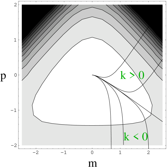
Figure 1: Solutions of the equation of motion for the N=2 SUGRA dual superimposed on the value of the superpotential (lighter regions correspond to larger values) in the $\rho-m$ plane.

In order to interpret these flows in terms of the N=2 gauge theory one requires some criteria for distinguishing between acceptable and unacceptable flows. In [15] it has been proposed that the flows may be distinguished based on the behaviour of the potential and superpotential along the flows. In particular, extrapolating from finite temperature situations where there are requirements for consistent black hole solutions, the author has proposed that only flows where the scalar potential is bounded above all along the flow are physical. This seems intuitive since these are flows that begin at the origin of the $\rho-m$ plane at large $y$ (that is they look like the N=4 theory in the UV) and then flow away from the origin, in directions where the potential falls, to large VEVs at small $y$ (the field theory IR).

To discuss this criteria for the flows of Fig.1 it is sensible to formulate boundary conditions that are easily interpretable in the field theory. In the field theory it is natural to start at some UV scale with a fixed mass and look for RG flows that correspond to different positions on the moduli space of the theory. Thus in the SUGRA we should fix $m$ at some $y=y_{UV}$ and look at flows with varying $\rho$. We are therefore taking initial conditions on a vertical slice through Fig 1. We are then interested in the behaviour of the potential along the flow to lower $y$. We plot the evolution of the potential (and superpotential) for several values of $y$ along such flows using numerical solutions of the field equations in Fig.2.

Figure 2: The potential and superpotential evaluated at varying $y$ along a set of flows in the N=2 theory starting at $y_{UV}=0.1$ with $m=0.1$ and varying $\rho(y_{UV})$.

The behaviour is that all flows which start with $\rho(y_{UV})$ greater than the value on the $k=0$ “ridge flow” eventually meet a positive potential wall, and hence by the conditions in [15] any flows with $k>0$ are to be considered unphysical. That the $k=0$ curve is the critical curve where this behaviour ends is clear from Fig 1 since only for the $k>0$ curves do the flows reach the singular behaviour of the superpotential which corresponds to that of the potential.

It seems likely therefore that the flows with $k\leq 0$ correspond to the RG flows of different points of the field theory moduli space. There is some evidence to suggest this is true. For the curves $k<0$, as can be seen in Fig 1, the flows asymptotically approach $\rho\rightarrow-\infty$ and $m\rightarrow$ constant. Evaluating the potential eq.(7) in this limit shows that the first term in the potential dominates and the potential becomes independent of $m$. Thus these flows asymptotically see the same potential suggesting a moduli space. That the different flows approach the asymptotic form of the potential at different rates with respect to $y$ is perhaps an indication that in the field theory different points on the moduli space have a different scale $tr\phi_{3}^{2}$ at which the gauge symmetry is broken, $SU(N)\rightarrow U(1)^{N-1}$. The singular point on the N=2 moduli space, where the U(1) couplings diverge, should naturally be equated with a special or extremal flow. The obvious such flow is the case $k=0$ which follows the crest of the ridge on the superpotential [15, 17]. These identifications can only be tentative based on the analysis so far. In [17] further evidence was provided by lifting the 5$d$ SUGRA solution to a 10$d$ SUGRA solution. This allows the authors to evaluate the gauge coupling (corresponding to the VEVs of the singlet scalars amongst the 42 scalars in the 5$d$ SUGRA theory - in the 5$d$ theory they do not enter the potential and so their VEVs can not be determined). They find that the coupling diverges on the $k=0$ flow but runs to a constant elsewhere which seems in accord with the field theory although the functional dependence of the coupling on the moduli space has not been reproduced.

We next move on to consider breaking the N=2 theory to the N=1 theory by the inclusion of the mass term $M$. In the field theory we expect to be pinned at the singular point and indeed we will see that the SUGRA flows pick out the $k=0$ flow providing further evidence for the above identification of the flows with the N=2 moduli space.

3.2 N=1 Flows

Flows with non-zero $M$ are expected to correspond to N=1 super-Yang-Mills theories. We begin by looking at theories which are N=2 SYM plus a small mass $M$ in the UV that breaks the supersymmetry to N=1. We again, in the SUGRA, fix $m$ and $M$ at some $y=y_{UV}$ and look at flows with varying $\rho(y_{UV})$. We are then interested in the behaviour of the potential along the flow to lower $y$. In Fig.3 we plot the evolution of the potential (and superpotential) for several values of $y$ along such flows using numerical solutions of the field equations with $M(y_{UV})=0.1m(y_{UV})$.

Figure 3: Plots of $V$ and $W$ at varying $y$ in the N=1 model with flows starting at $y_{UV}=0.1$ and $M(y_{UV})=0.1m(y_{UV})$ with $m(y_{UV})=0.1$ and varying $\rho(y_{UV})$. The pinning of the potential on the N=2 critical flow is apparent as one approaches the IR.

From Fig.3 it is apparent that as we proceed towards the IR all the flows except the flow along the ridge of the superpotential eventually meet a positive “barrier” in the potential. Thus only the single ridge flow is allowed by the criteria for distinguishing flows discussed above. This matches our expectations from field theory where we expected the theory to become pinned at the singular point of the N=2 theory previously identified with that ridge flow.

The existence of a ridge flow seems to be confirmed by the analysis of the numerical solutions of the equations of motion. One can indeed distinguish two sets of solutions with radically different behaviours. The change of behaviour seems to take place for a negative value of the $\rho(y_{UV})$, which should correspond to the position of the ridge flow. This is consistent with what shown in Fig 3. In Fig. 4 we plot $M,m$ and $\rho$ as functions of $y$ for two values of $\rho(y_{UV})$ on either sides of the ridge flow. In analogy with the N=2 theory case, we will call the ridge flow $k=0$, while $k<0$ and $k>0$ will indicate the flows on the left and on the right of it, respectively. Notice however that here the parameter $k$ is not related with any precise form of the solutions.

Figure 4: The evolution of the individual fields $\rho,m,M$ with $y$. The left hand plot corresponds to a $k<0$ flow, the right hand plot to $k>0$. Initial conditions are as in Fig 3 above.

Unfortunately it is not very easy to reproduce the behaviour of the ridge flow. Numerically, it is very difficult to pick out the precise value of $\rho(y_{UV})$ corresponding to the ridge flow, and analytically, it is not easy to solve the equations of motion even in the IR limit. It is even hard to guess the correct asymptotic behaviour of the fields. For example, one would have hoped to recover a logarithmic behaviour like in the N=1 or N=2 case, but this possibility seems to be ruled out. This is confirmed by the plots in Fig. 5 below, where the behaviour of the ratios of the various fields as a function of $y$ are shown. The existence of, and distinction between, the ridge flow and the two classes of flows to either side are clear, but note that close to the ridge flow there is no linear relation between the fields.

Figure 5: The evolution of the ratios $\rho/m,m/M$ and $\rho/M$ with $y$ as function of $\rho(y_{UV})$.

From Fig. 4, one can see that our solutions are all singular in the IR. It is then natural to ask whether they correspond to physical or unphysical flows. The expectation is that only the ridge flow should be physical. Unfortunately we can explicitly check only the case $k<0$, where we can extract information from the IR asymptotic behaviours

$$m \sim \mbox{const},$$ (26)

$$M \sim -\frac{3}{7}\log|y-y_{0}|+\mbox{const},$$ (27)

$$\rho \sim \frac{\sqrt{6}}{14}\log|y-y_{0}|+\mbox{const},$$ (28)

$$\phi \sim \frac{1}{7}\log|y-y_{0}|+\mbox{const}.$$ (29)

Notice in particular the logarithmic divergence of the field $\phi$: $\phi\sim A\log|y-y_{0}|$. Indeed for logarithmically divergent flows, the criterion proposed in [15] to select physically sensible solutions seems to pick up flows with $A\geq 1/4$ [16]. This rules out the $k<0$ flows for which $A=1/7$.

For the ridge and the $k>0$ flows we can rely only on the numerical behaviour of the potential and the superpotential, that, as observed above, seem to allow only for one physical flow, the ridge.

Finally let us consider the situation where the two masses $m$ and $M$ are of the same order. In field theory we expect to recover pure N=1 SYM. In particular the vacuum state should evolve into the N=1 solution of [14]. From the supergravity point of view the N=1 and the N=2 theories can be distinguished by the scalars one has to turn on. As discussed in [14], in the N=1 solution the scalar $\rho$ is set to zero. In this case, the supergravity mode corresponding to the mass term for the scalar fields corresponds to the stringy mode only and it is therefore not present in the 5$d$ supergravity Lagrangian. Thus we expect that as we increase $M(y_{UV})$ the ridge line flow should smoothly move to the value $\rho=0$.

Figure 6: The evolution of the position of the critical curve with varying $M(y_{UV})$ from the N=2 to pure N=1 theory.

This is indeed the case, as can be seen in Fig. 6 where we have plotted the potential and superpotential as a function of the UV values of $\rho$, in the deep IR (small $y$), for three different values of the ratio $M(y_{UV})/m(y_{UV})$. $M(y_{UV})=m(y_{UV})/\sqrt{2}$ corresponds to pure N=1 SYM and the superpotential ridge has indeed moved to $\rho=0$.

4 Discussion

We have calculated the 5$d$ SUGRA scalar potential corresponding to fields dual to scalar and fermion masses and a scalar VEV for the lightest chiral multiplet in N=4 SYM softly broken in a cascade to N=2 and then N=1 SYM. We have found numerical solutions of the resulting SUGRA equations of motion and used the criteria that the potential must fall all along the flow, as suggested in [15], to distinguish physical flows. Interpreting these flows in terms of the dual field theory leads to a pleasing picture of the transition between the N=2 flows of [15, 17] and the N=1 flows of [14]. The N=2 theory has a moduli space and thus there is a class of flows in SUGRA which are physically acceptable. The extremal curve has been identified with the singular point on the moduli space. When a small mass is introduced to break the theory to N=1 SYM all these flows except the extremal flow have their potential lifted in the IR which, according to the criteria above, indicates they are unphysical. We thus see the unique vacuum of the N=1 theory emerging from the N=2 theory and, as expected from the field theory, the N=1 theory is pinned at the singular point on the N=2 moduli space. As the two perturbing masses (the one that sets the breaking N=4 to N=2 and the one that further breaks to N=1) become of the same order, leaving N=1 SYM in the IR, the extremal flow is seen to smoothly move to the origin of the N=2 theory’s moduli space, again in agreement with field theory expectations.

A number of issues remain for future investigation. The N=1 theory is expected to have a gaugino condensate, represented in SUGRA by a further scalar we have neglected in our discussion. Although the potential is easy to compute, including this scalar would raise the dimension of the parameter space of flows making analysis harder, so we prefer to leave it for future analysis. From the field theory we also expect to see monopole condensation and confinement (in the field theory of the softly broken N=2 theory there are $N^{2}-1$ different string tensions one might hope to see a SUGRA dual of [23]). The solutions we present have an IR singularity so we could hope that the ridge flow solution exhibits confinement. However we have no means to check the behaviour without explicit solutions. The usual methods one can apply in supergravity to check confinement, such as the computation of a Wilson loop [32] or the the evaluation of the spectrum of scalars [30, 31], all require at least the knowledge of the IR asymptotic behaviour of the solution. In this respect it may be profitable to study the lift of the 5$d$ SUGRA to the full 10$d$ theory where explicit solutions may be more readily obtainable. The 10$d$ solutions would also allow study of the running of the gauge coupling which would provide further checks of our interpretation.

AcknowledgementsM.P. would like to thank A. Zaffaroni and G. Salam for very useful discussions and comments. M.P is partially supported by INFN and MURST, and by the European Commission TMR program ERBFMRX-CT96-0045, wherein she is associated to Imperial College, London, and by the PPARC SPG grant 613. N.E is grateful for the support of a PPARC Advanced Fellowship.

References

- [1] J. Maldacena, Adv. Theor. Math. Phys. 2 (1998) 231, hep-th/9711200.
- [2] S.S. Gubser, I.R. Klebanov and A.M. Polyakov, Phys. Lett. B428 (1998) 105, hep-th/9802109.
- [3] E. Witten, Adv. Theor. Math. Phys. 2 (1998) 253, hep-th/9802150.
- [4] L. Girardello, M. Petrini, M. Porrati and A. Zaffaroni, JHEP 9812 (1998) 022, hep-th/9810126.
- [5] J. Distler and F. Zamora, Adv. Theor. Math. Phys. 2 (1998) 1405, hep-th/9810206.
- [6] A. Khavaev, K. Pilch and N. P. Warner, New Vacua of Gauged N=8 Supergravity, hep-th/9812035.
- [7] A. Karch, D. Lüst and A. Miemiec, Phys. Lett. B454 (1999) 265, hep-th/9810254.
- [8] A. Kehagias and K. Sfetsos, Phys. Lett. B454 (1999) 270,hep-th/9902125; S. S. Gubser, Dilaton-driven confinement, hep-th/9902155; N. R. Constable and R. C. Myers, JHEP 9911 (1999) 020, hep-th/9905081.
- [9] L. Girardello, M. Petrini, M. Porrati and A. Zaffaroni, JHEP 9905 (1999) 026, hep-th/9903026.
- [10] S. Nojiri and S. D. Odintsov, Phys.Lett. B449 (1999) 39,hep-th/9812017; B458 (1999) 226, hep-th/9904036.
- [11] D. Z. Freedman, S. S. Gubser, K. Pilch and N. P. Warner,Renormalization Group Flows from Holography–Supersymmetry and a c-Theorem, hep-th/9904017.
- [12] D. Z. Freedman, S. S. Gubser, K. Pilch and N. P. Warner,Continuous distributions of D3-branes and gauged supergravity, hep-th/9906194;
- [13] A. Brandhuber and K. Sfetsos, Wilson loops from multicentre and rotating branes, mass gaps and phase structure in gauge theories, hep-th/9906201; I. Chepelev and R. Roiban, Phys.Lett. B462 (1999) 74, hep-th/9906224. I. Bakas and K. Sfetsos, Nucl.Phys. B573 (2000) 768, hep-th/9909041.
- [14] L. Girardello, M. Petrini, M. Porrati and A. Zaffaroni, Nucl.Phys. B569 (2000) 451, hep-th/9909047.
- [15] S.S. Gubser Curvature Singularities: the Good, the Bad, and the Naked, hep-th/0002160.
- [16] M. Petrini and A. Zaffaroni, The Holographic RG flow to conformal and non-conformal theory, hep-th/0002172.
- [17] K. Pilch and N. P. Warner N=2 Supersymmetric RG Flows and the IIB Dilaton, hep-th/0004063.
- [18] A. Brandhuber and K. Sfetsos An N=2 gauge theory and its supergravity dual, hep-th/0004148.
- [19] A. Peet and J. Polchinski, Phys.Rev. D59 (1999) 065011, hep-th/9809022.
- [20] C. V. Johnson, A. W. Peet and J. Polchinski, Phys. Rev. D61 (2000) 086001, hep-th/9911161.
- [21] R.C. Myers, JHEP 9912 (1999) 022, hep-th/9910053.
- [22] J. Polchinski and M. J. Strassler, The String Dual of a Confining Four-Dimensional Gauge Theory, hep-th/0003136.
- [23] N. Seiberg and E. Witten, Nucl. Phys. B431 (1994) 484, hep-th/9408099; M.R. Douglas and S.H. Shenker Nucl. Phys. B447 (1995) 271, hep-th/9503163.
- [24] C. Vafa and E. Witten, Nucl. Phys. B431 (1994) 3, hep-th/9408074; R. Donagi and E. Witten, Nucl. Phys. B460 (1996) 299, hep-th/9510101; N. Dorey JHEP 9907 (1999) 021, hep-th/9906011; N. Dorey and S. Prem Kumar, JHEP 0002 (2000) 006, hep-th/0001103.
- [25] M. Günaydin, L.J. Romans and N.P. Warner, Phys. Lett. B154 (1982) 68; M. Pernici, K. Pilch and P. van Nieuwenhuizen, Nucl. Phys. B259 (1985) 460.
- [26] M. Günaydin, L.J. Romans and N.P. Warner, Nucl. Phys. B272 (1986) 598.
- [27] K. Skenderis and P. K. Townsend, Phys. Lett. B468 (1999) 46, hep-th/9909070.
- [28] V. Balasubramanian, P. Kraus, A. Lawrence and S. Trivedi, Phys. Rev. D59 (1999) 104021, hep-th/9808017.
- [29] I. R. Klebanov and E. Witten, Nucl. Phys. B556 (1999) 89, hep-th/9905104.
- [30] E. Witten, Adv.Theor.Math.Phys. 2 (1998) 505, hep-th/9803131.
- [31] C. Csaki, H. Ooguri, Y. Oz and J. Terning, JHEP 9901 (1999) 017, hep-th/9806021.
- [32] J. Maldacena, Phys. Rev. Lett. 80 (1998) 4859, hep-th/9803002