Hamiltonian structure and gauge symmetries
of Poincaré gauge theory

Abstract

This is a review of the constrained dynamical structure of Poincaré gauge theory which concentrates on the basic canonical and gauge properties of the theory, including the identification of constraints, gauge symmetries and conservation laws. As an interesting example of the general approach we discuss the teleparallel formulation of general relativity.

1. Introduction

Despite its successes in describing known macroscopic gravitational phenomena, Einstein’s general relativity (GR) still lacks the status of a fundamental microscopic theory. This is so because the theory admits singular solutions under very general assumptions, and all attempts to quantize GR encounter serious difficulties. Among various attempts to overcome these problems, gauge theories of gravity are especially attractive, as they are based on the concept of gauge symmetry which has been very successful in the foundation of other fundamental interactions. The importance of the Poincaré symmetry in particle physics leads one to consider the Poincaré gauge theory (PGT) as a natural framework for a description of the gravitational phenomena [1–6] (for more general attempts, see [7]).

In this paper we give an introduction to PGT and general Dirac’s formalism, and a review of the constrained dynamical structure of PGT, aimed at a fairly general audience. We begin our exposition by giving a short outline of PGT in Sec. 2. In the next section we introduce basic concepts of Dirac’s Hamiltonian formalism, which are essential for a clear understanding of the canonical and gauge structure of any gauge theory. Then, we discuss the construction of the Hamiltonian and the algebra of constraints in the general PGT (Sec. 4), derive the related generator of Poincaré gauge symmetry (Sec. 5), and introduce the important concept of energy (and other conserved charges) on the basis of the asymptotic structure of spacetime (Sec. 6). The teleparallel form of GR is an interesting limit of PGT, both theoretically and observationally; its canonical properties are discussed in Sec. 7. Section 8 is devoted to concluding remarks.

Our general conventions, with some exceptions in Sect. 3, are the following: the Latin indices refer to the local Lorentz frame, whereas the Greek indices refer to the coordinate frame; the first letters of both alphabets $(a,b,c,\dots;\alpha,\beta,\gamma,\dots)$ run over $1,2,3$, while the middle alphabet letters $(i,j,k,\dots;\mu,\nu,\l,\dots)$ run over $0,1,2,3$; $\eta_{ij}=(+,-,-,-)$, and $\varepsilon^{ijkl}$ is completely antisymmetric tensor normalized to $\varepsilon^{0123}=+1$.

2. Poincaré gauge theory

It is well known that the existence and interaction of certain fields, such as the electromagnetic field, can be closely related to invariance properties of the theory. Thus, for instance, if the Lagrangian of matter fields is invariant under phase transformations with constant parameters $\alpha$, the electromagnetic field can be introduced by demanding the invariance under the extended, local transformations, obtained by replacing $\alpha$ with a function of spacetime points, $\alpha\to\alpha(x)$.

On the other hand, it is much less known that Einstein’s GR is invariant under local Poincaré transformations. This property is based on the principle of equivalence, and gives a rich physical content to the concept of local (or gauge) symmetry. Instead of thinking of local Poincaré symmetry as derived from the principle of equivalence, the whole idea can be reversed, in accordance with the usual philosophy of gauge theories. When gravitational field is absent, it has become clear from a host of experiments that the underlying symmetry of fundamental interactions is given by the Poincaré group. If we now want to make a physical theory invariant under local Poincaré transformations, it is necessary to introduce new, compensating (or gauge) fields, which, in fact, represent the gravitational interaction [1–6].

Global Poincaré symmetry. In physical processes at low energies gravitational field does not have a significant role, since the gravitational interaction is extremely weak. The spacetime without gravity is described by the special relativity theory (SR), and its mathematical structure corresponds to Minkowski space $M_{4}$. Any physical observer in $M_{4}$ uses some reference frame, endowed with coordinates $x^{\mu}$ $(\mu=0,1,2,3)$, serving to identify physical events. An inertial observer can always choose global inertial coordinates, such that the infinitesimal interval has the form $ds^{2}=\eta_{\mu\nu}dx^{\mu}dx^{\nu}$, where $\eta_{\mu\nu}=(1,-1,-1,-1)$ is the metric tensor. The equivalence of inertial reference frames is expressed by the global (rigid) Poincaré symmetry $P(1,3)$ in $M_{4}$.

At each point of $M_{4}$, labeled by coordinates $x^{\mu}$, one can define an inertial laboratory by a local Lorentz frame — a set of four orthonormal, tangent vectors $\hbox{\boldmath$e$}_{i}(x)$, $\hbox{\boldmath$e$}_{i}\cdot\hbox{\boldmath$e$}_{j}=\eta_{ij}$, called the tetrad. In global inertial coordinates $x^{\mu}$, one can always choose the tetrad such that it coincides with a coordinate frame $\hbox{\boldmath$e$}_{\mu}(x)$ (a set of four vectors, tangent to coordinate lines at $x$), i.e. $\hbox{\boldmath$e$}_{i}=\delta_{i}^{\mu}\hbox{\boldmath$e$}_{\mu}$. Here, the Latin indices $(i,j,...)$ refer to local Lorentz frames, while the Greek indices $(\mu,\nu,...)$ refer to coordinate frames.

The physics of fundamental interactions is successfully described by Lagrangian field theory. Dynamical variables in this theory are fields $\phi(x)$, and dynamics is determined by a function of fields and their derivatives, ${\cal L}(\phi,\partial_{k}\phi)$, called the Lagrangian. The action integral $I=\int d^{4}x{\cal L}$ is invariant under an arbitrary spacetime transformation $x^{\prime m}=x^{m}+\xi^{m}$, $\phi^{\prime}(x)=\phi(x)+\delta_{0}\phi(x)$, provided the Lagrangian satisfies the condition [1]

$$\delta_{0}{\cal L}+\partial_{m}(\xi^{m}{\cal L})=0\,,$$ (2.1)

where $\delta_{0}{\cal L}\equiv(\partial{\cal L}/\partial\phi)\delta_{0}\phi+(\partial{\cal L}/\partial\phi_{,k})\delta_{0}\phi_{,k}$. Note that this condition can be, in fact, relaxed, by allowing an arbitrary four–divergence to appear on the right hand side. The Lagrangian ${\cal L}$ satisfying the above invariance condition is called an invariant density.

Consider now a matter field $\psi(x)$ in spacetime, referred to a local Lorentz frame. Its transformation law under the global Poincaré transformations $\xi^{m}=\o^{m}{{}_{n}}x^{n}+\varepsilon^{m}$ has the form

$$\delta_{0}\psi=\bigl{(}\hbox{${1\over 2}$}\o\cdot M+\varepsilon\cdot P\bigr{)}\psi=\bigl{(}\hbox{${1\over 2}$}\o\cdot\Sigma+\xi\cdot P\bigr{)}\psi\,,$$

where $M_{mn}=x_{m}\partial_{n}-x_{n}\partial_{m}+\Sigma_{mn}$ and $P_{m}=-\partial_{m}$ are the Poincaré generators, and $\Sigma_{mn}$ is the spin matrix. Using the invariance condition (2.1), one finds that the invariance of the Lagrangian ${\cal L}_{M}(\psi,\partial_{k}\psi)$ under $P(1,3)$ leads to the conservation of energy–momentum and angular momentum currents.

Localization of Poincaré symmetry leads to Poincaré gauge theory of gravity, in which both energy–momentum and spin currents of matter fields are naturally included into gravitational dynamics, in contrast to GR.

Local Poincaré symmetry. We now describe the process of transition from global to local Poincaré symmetry, and find its relation to the gravitational interaction. Other spacetime symmetries [de Sitter, conformal, etc.] can be treated in an analogous manner.

Consider a Lagrangian for matter fields, ${\cal L}_{M}={\cal L}_{M}(\psi,\partial_{k}\psi)$, defined with respect to a local Lorentz frame and invariant under $P(1,3)$. If we now generalize global Poincaré transformations by replacing ten constant group parameters $\o^{m}{{}_{n}},\varepsilon^{m}$ with some functions of spacetime points, the invariance condition (2.1) is violated. The violation of (local) invariance can be compensated by certain modifications of the original theory. After introducing the covariant derivative,

$$\nabla_{k}\psi=h_{k}{{}^{\mu}}\nabla_{\mu}\psi=h_{k}{{}^{\mu}}\bigl{(}\partial_{\mu}+\hbox{${1\over 2}$}A^{ij}{{}_{\mu}}\Sigma_{ij}\bigr{)}\psi\,,$$ (2.2a)

where $$h_{k}{{}^{\mu}} A^{ij}{{}_{\mu}}$$ and are the compensating fields, the modified, invariant Lagrangian for matter fields takes the form

$$\widetilde{\cal L}_{M}=b{\cal L}_{M}(\psi,\nabla_{k}\psi)\,,$$ (2.2b)

where $b=\det(b^{k}{{}_{\mu}})$, and $b^{k}{{}_{\mu}}$ is the inverse of $h_{k}{{}^{\mu}}$. It is obtained from the original Lagrangian ${\cal L}_{M}(\psi,\partial_{k}\psi)$ in two steps:

• by replacing $\partial_{k}\psi\to\nabla_{k}\psi$ (minimal coupling), and

• multiplying ${\cal L}_{M}$ by $b$.

The Lagrangian $\widetilde{\cal L}_{M}$ satisfies Eq. (2.1) by construction, hence it is an invariant density.

The matter Lagrangian is made invariant under local transformations by introducing compensating fields. In order to construct an invariant Lagrangian for the new fields $b^{k}{{}_{\mu}}$ and $A^{ij}{{}_{\mu}}$, we introduce the corresponding field strengths,

related to the Lorentz and translation subgroups of $P(1,3)$, respectively. The new Lagrangian must be an invariant density depending only on the Lorentz and translation field strengths, so that the complete Lagrangian of matter and gauge fields has the form

$$\widetilde{\cal L}=b{\cal L}_{F}(F^{ij}{{}_{kl,}}F^{i}{{}_{kl}})+b{\cal L}_{M}(\psi,\nabla_{k}\psi)\,.$$ (2.4)

Up to this point, we have not given any geometric interpretation to the new, compensating fields $b^{k}{{}_{\mu}}$ and $A^{ij}{{}_{\mu}}$. Such an interpretation is possible and useful, and it leads to a new understanding of gravity.

Riemann–Cartan geometry. Now, we introduce some basic geometric concepts in order be able to understand the geometric meaning of PGT [2, 8].

Spacetime is often described as a “four–dimensional continuum”. In SR, it has the structure of Minkowski space $M_{4}$. In the presence of gravity spacetime can be divided into “small, flat pieces” in which SR holds (on the basis of the principle of equivalence), and these pieces are “sewn together” smoothly. Although spacetime looks locally like $M_{4}$, it may have quite different global properties. Mathematical description of such four–dimensional continuum is given by the concept of a differentiable manifold.

We assume that spacetime has a structure of a differentiable manifold $X_{4}$. On $X_{4}$ one can define differentiable mappings, tensors, and various algebraic operations with tensors at a given point (addition, multiplication, contraction). However, comparing tensors at different points requires some additional structure on $X_{4}$: the law of parallel transport, defined by a linear (or affine) connection $\Gamma$. An $X_{4}$ equipped with $\Gamma$ is called linearly connected space, $L_{4}=(X_{4},\hbox{\boldmath$\Gamma$})$. Linear connection is equivalently defined by the covariant derivative $D$; thus, for instance, $D_{\rho}A^{\mu}=\partial_{\rho}A^{\mu}+\Gamma^{\mu}_{\l\rho}A^{\l}$.

Linear connection is not a tensor, but its antisymmetric part defines a tensor called the torsion tensor: $T^{\mu}{{}_{\l\rho}}=\Gamma^{\mu}_{\rho\l}-\Gamma^{\mu}_{\l\rho}$.

Parallel transport is a path dependent concept. If we parallel transport a vector around an infinitesimal closed path, the result is proportional to the Riemann curvature tensor: $R^{\mu}{{}_{\nu\l\rho}}=\partial_{\l}\Gamma_{\nu\rho}^{\mu}+\Gamma_{\sigma\l}^{\mu}\Gamma_{\nu\rho}^{\sigma}-(\l\leftrightarrow\rho)$.

On $X_{4}$ one can define metric tensor $g$ as a symmetric, nondegenerate tensor field of type $(0,2)$. After that we can introduce the scalar product of two tangent vectors and calculate lengths of curves, angles between vectors, etc. Linear connection and metric are geometric objects independent of each other. The differentiable manifold $X_{4}$, equipped with linear connection and metric, becomes linearly connected metric space $(L_{4},\hbox{\boldmath$g$})$.

In order to preserve lengths and angles under parallel transport in $(L_{4},\hbox{\boldmath$g$})$, one can impose the metricity condition

$$-Q_{\mu\nu\l}\equiv D_{\mu}g_{\nu\l}=\partial_{\mu}g_{\nu\l}-\Gamma_{\nu\mu}^{\rho}g_{\rho\l}-\Gamma_{\l\mu}^{\rho}g_{\nu\rho}=0\,,$$ (2.5)

which relates $\Gamma$ and $g$. The requirement of vanishing nonmetricity $Q$ establishes local Minkowskian structure on $X_{4}$, and defines a metric compatible linear connection.

A space $(L_{4},\hbox{\boldmath$g$})$ with the most general metric compatible linear connection $\Gamma$ is called Riemann–Cartan space $U_{4}$. If the torsion vanishes, $U_{4}$ becomes Riemann space $V_{4}$ of GR; if, alternatively, the curvature vanishes, $U_{4}$ becomes Weitzenböck’s teleparallel space $T_{4}$. Finally, the condition $\,R^{\mu}{{}_{\nu\l\rho}}=0\,$ transforms $V_{4}$ into Minkowski space $M_{4}$, and $\,T^{\mu}{{}_{\l\rho}}=0\,$ transforms $T_{4}$ into $M_{4}$ (Figure 1).

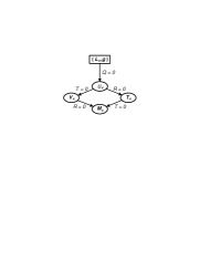
Figure 1: Classification of spaces satisfying the metricity condition

The choice of basis in a tangent space is not unique. Coordinate frame $\hbox{\boldmath$e$}_{\mu}$ and local Lorentz frame $\hbox{\boldmath$e$}_{i}$ are of particular practical importance. Every tangent vector $u$ can be expressed in both frames: $\hbox{\boldmath$u$}=u^{\mu}\hbox{\boldmath$e$}_{\mu}=u^{i}\hbox{\boldmath$e$}_{i}$. In particular, $\hbox{\boldmath$e$}_{i}=e_{i}{{}^{\mu}}\hbox{\boldmath$e$}_{\mu}$ and $\hbox{\boldmath$e$}_{\mu}=e^{i}{{}_{\mu}}\hbox{\boldmath$e$}_{i}$. As a consequence, we find that $u^{i}=e^{i}{{}_{\mu}}u^{\mu}$, $u^{\mu}=e_{i}{{}^{\mu}}u^{i}$. We denote the connection components with respect to coordinate and local Lorentz frames as $\Gamma^{\mu}_{\l\rho}$ and $\o^{ij}{{}_{\mu}}$, respectively.

Linear connection and metric are geometric objects independent of the choice of frame. Their components are defined with respect to a frame and are, clearly, frame–dependent.

Interpretation of PGT. The final result of the analysis of PGT is the construction of the invariant Lagrangian (2.4). It is achieved by introducing new fields $h_{i}{{}^{\mu}}$ (or $b^{k}{{}_{\nu}}$) and $A^{ij}{{}_{\mu}}$, which are used to construct the covariant derivative $\nabla_{k}$ and the field strengths $F^{ij}{{}_{\mu\nu}}$ and $F^{i}{{}_{\mu\nu}}$. This theory can be thought of as a field theory in $M_{4}$. However, geometric analogies are so strong, that it would be unnatural to ignore them. The following properties are essential for the geometric interpretation of PGT:

• the Lorentz gauge field $A^{ij}{{}_{\mu}}$ can be identified with the Lorentz connection $\o^{ij}{{}_{\mu}}$, or, equivalently, the covariant derivative $\nabla_{\mu}(A)$ can be identified with $D_{\mu}(\o)$;

• the translation gauge field $b^{k}{{}_{\mu}}$ can be identified with the tetrad $e^{k}{{}_{\mu}}$;

• local Lorentz symmetry of PGT implies the metricity condition (2.5).

Consequently, PGT has the geometric structure of Riemann–Cartan space $U_{4}$.

It is not difficult to prove that the field strengths $F^{i}{{}_{\mu\nu}}$ and $F^{ij}{}_{\mu\nu}$ represent geometrically the torsion $T^{\l}{{}_{\mu\nu}}$ and the curvature $R^{\l}{}_{\tau\mu\nu}$, respectively.

Since Riemann–Cartan space has locally the structure of $M_{4}$, it follows that PGT is consistent with the principle of equivalence [9]. Thus, PGT is a gauge approach to the theory of gravity, possessing a transparent geometric and physical interpretation.

3. Constrained Hamiltonian dynamics

Despite many successes of quantum theory in describing basic physical phenomena, one is continually running into difficulties in some specific physical situations. Thus, all attempts to quantize the theory of gravity encounter serious difficulties. In order to find a solution of these problems, it seems to be useful to reconsider the fundamental principles of classical dynamics. In this context, the principles of Hamiltonian dynamics are seen to be of great importance for a basic understanding of both classical and quantum theory.

In gauge theories the number of dynamical variables in the action is larger than the number of physical variables. The presence of unphysical variables is closely related to the existence of gauge symmetries. In the Hamiltonian formalism dynamical systems of this type are characterized by the presence of constraints. Here, we present the basic ideas of the constrained Hamiltonian dynamics [10, 11, 12].

Primary constraints. In order to simplify the exposition we start by considering a classical system of particles, described by coordinates $q_{i}\,\,(i=1,2,...,N)$ and the action $I=\int dt\,L(q,\dot{q})$. To go over to the Hamiltonian formalism we introduce, in the usual way, the momentum variables:

$$p_{i}={\partial L\over\partial\dot{q}_{i}}\equiv f_{i}(q,\dot{q})\qquad(i=1,2,...,N)\,.$$ (3.1)

In simple dynamical theories these relations can be inverted, so that all velocities can be expressed in terms of the coordinates and momenta, whereupon one can simply define the Hamiltonian function. However, for many interesting theories such an assumption would be too restrictive. Therefore, we shall allow for the possibility that momentum variables are not independent functions of velocities, i.e. that there exist constraints:

$$\phi_{m}(q,p)=0\qquad(m=1,2,...,P)\,.$$ (3.2a)

The variables $$(q,p) \Gamma \Gamma_{1} \Gamma$$ are local coordinates on the phase space . The relations (3.2a) are called primary constraints; they determine a subspace of , in which the time development of a dynamical system takes place.

The geometric structure of the subspace $\Gamma_{1}$ can be very complicated. If $(i)$ the rank of the matrix ${\cal J}=\partial\phi_{m}/\partial(q,p)$ is constant on $\Gamma_{1}$, and $(ii)$ all the constraint functions $\phi_{m}$ are independent (irreducible), then the Jacobian ${\cal J}$ is of rank $P$ on $\Gamma_{1}$. Accordingly, the dimension of $\Gamma_{1}$ is well defined and equal to $2N-P$.

Weak and strong equalities. At this stage we introduce the useful notions of weak and strong equality. Let $F(q,p)$ be a function which is defined and differentiable in a neighborhood ${{\cal O}}_{1}\subseteq\Gamma$ containing the subspace $\Gamma_{1}$. If the restriction of $F(q,p)$ on $\Gamma_{1}$ vanishes, we say that $F$ is weakly equal to zero: $F(q,p)\approx 0$. If the function $F$ and all its first derivatives vanish on $\Gamma_{1}$, than $F$ is strongly equal to zero: $F(q,p)=0$. For strong equality we shall use the usual equality sign. This definition is especially useful in the analysis of the equations of motion, which contain derivatives of functions on $\Gamma_{1}$.

By using these conventions the relations (3.2a) can be written as weak equalities:

$$\phi_{m}(q,p)\approx 0\qquad(m=1,2,...,P)\,.$$ (3.2b)

It is now interesting to clarify the relation between strong and weak equalities: if $F(q,p)$ vanishes weakly, $F\approx 0$, what can one say about the derivatives of $F$ on $\Gamma_{1}$? By use of the general method of calculus of variations with constraints, one can show that $F\approx 0$ implies $F-\l^{m}\phi_{m}\approx{\cal O}$, where $\l^{m}$ are some multipliers, and ${\cal O}$ is a quantity whose derivatives are weakly vanishing: it can be zero, a constant, or second or higher power of a constraint. For theories in which the constraint functions $\phi_{m}$ satisfy the above regularity condition $(i)$ and $(ii)$, one can show that ${\cal O}=0$ [11].

Hamiltonian. Consider now the quantity

$$H_{c}=p_{i}\dot{q}_{i}-L(q,\dot{q})\,.$$ (3.3)

By making variations in $q$ and $\dot{q}$ one finds that $H_{c}$ can be expressed in terms of $q$’s and $p$’s only, independent of velocities. Expressed in this way it becomes the canonical Hamiltonian. Since $H_{c}$ is not uniquely defined in the presence of constraints, it is natural to introduce the total Hamiltonian

$$H_{T}=H_{c}+u^{m}\phi_{m}\,,$$ (3.4)

where $u^{m}$’s are, at this stage, arbitrary multipliers. By varying this expression with respect to $(u,q,p)$ one obtains the constraints (3.2) and the Hamiltonian equations of motions involving arbitrary multipliers. The Hamiltonian equations for an arbitrary dynamical quantity $g(q,p)$ can be written in the form

$$\dot{g}=\{g,H_{c}\}+u^{m}\{g,\phi_{m}\}\approx\{g,H_{T}\}\,,$$ (3.5)

where $\{X,Y\}$ is the Poisson bracket (PB) of $X$ and $Y$.

Equations (3.5) describe the motion of a system in the subspace $\Gamma_{1}$ of dimension $2N-P$. The motion is described by $2N$ coordinates $(q,p)$ satisfying $P$ constraints; as a consequence, there appear $P$ multipliers in the evolution equations. Explicit elimination of some coordinates is possible, but it may lead to a violation of locality and/or covariance.

Consistency conditions. A basic consistency of the theory requires that the primary constraints be conserved during the temporal evolution of the system:

$$\dot{\phi}_{m}=\{\phi_{m},H_{c}\}+u^{n}\{\phi_{m},\phi_{n}\}\approx 0\,.$$ (3.6)

If the equations of motion are consistent, the above conditions reduce to the one of the following three cases: $a)$ an identity, 0=0; $b)$ an equation independent of the multipliers, yielding a new, secondary constraint: $\chi(q,p)\approx 0$; $c)$ a restriction on the $u^{n}$’s.

If we find some secondary constraints in the theory, they also have to satisfy consistency conditions of the type (3.6). The process continues until all consistency conditions are exhausted. As a final result we are left with a number of new constraints, and a number of conditions on the multipliers.

Let us denote all the constraints in the theory as $\varphi_{s}\equiv(\phi_{m},\chi_{n})\approx 0$. These constraints define a subspace $\Gamma_{2}$ of the phase space $\Gamma$, such that $\Gamma_{2}\subseteq\Gamma_{1}$. The notions of weak and strong equalities are now defined with respect to $\Gamma_{2}$.

Since the consistency requirements lead, in general, to some conditions on the multipliers, the total Hamiltonian can be written in the form

$$H_{T}=H^{\prime}+v^{a}\phi_{a}\qquad(a=1,2,...,N^{\prime}_{1})$$ (3.7)

where $H^{\prime}=H_{c}+U^{m}\phi_{m}$, $U^{m}$ are determined and $v^{a}$ arbitrary multipliers.

Thus, even after all the consistency requirements are satisfied, we still have arbitrary functions of time in the theory. As a consequence, dynamical variables at some future instant of time are not uniquely determined by their initial values.

First class and second class quantities. A dynamical variable $R(q,p)$ is said to be first class (FC) if it has weakly vanishing PBs with all constraints in the theory: $\{R,\varphi_{s}\}\approx 0$. If $R$ is not first class, it is called second class. While the distinction between primary and secondary constraints is of little importance in the final form of the Hamiltonian theory, the property of being FC or second class is essential for the dynamical interpretation of constraints.

We have seen that (in a regular theory) any weakly vanishing quantity is strongly equal to a linear combination of constraints. Therefore, if the quantity $R(q,p)$ is FC, it satisfies the strong equality $\{R,\varphi_{s}\}=R_{s}{{}^{r}}\varphi_{r}$. From this one can infer, by virtue of the Jacoby identity, that the Poisson bracket of two FC constraints is also FC.

The quantities $H^{\prime}$ and $\phi_{a}$ in $H_{T}$ are FC. Thus, the number of independent functions of time $v^{a}(t)$ in $H_{T}$ is equal to the number of independent primary FC constraints $\phi_{a}$.

The presence of arbitrary multipliers in the equations of motion (and their solutions) means that the variables $(q(t),p(t))$ can not be uniquely determined from given initial values $(q(0),p(0))$; therefore, they do not have a direct physical meaning. Physical informations about a system can be obtained from functions $A(q,p)$, defined on constraint surface, that are independent of arbitrary multipliers; such functions are called (classical) observables. The physical state of a system at time $t$ is determined by the complete set of observables at that time.

In order to illustrate these ideas, let us consider a general dynamical variable $g(t)$ at $t=0$, and its change after a short time interval $\delta t$. The initial value $g(0)$ is determined by $(q(0),p(0))$. The value of $g(t)$ at time $\delta t$ can be calculated from the equations of motion: $g(\delta t)=g(0)+\delta t\{g,H_{T}\}$. Since the coefficients $v^{a}(t)$ in $H_{T}$ are completely arbitrary, we can take different values for these coefficients and obtain different values for $g(\delta t)$, the difference being of the form $\Delta g(\delta t)=\varepsilon^{a}\{g,\phi_{a}\}$, where $\varepsilon^{a}=\delta t(v_{2}^{a}-v_{1}^{a})$. This change of $g(\delta t)$ is unphysical, as $g_{1}(\delta t)$ and $g_{2}(\delta t)=g_{1}(\delta t)+\Delta g(\delta t)$ correspond to the same physical state. We come to the conclusion that primary FC constraints generate unphysical transformations of dynamical variables, known as gauge transformations, that do not change the physical state of the system.

Similarly, one can conclude that the quantity $\{\phi_{a},\phi_{b}\}$ is also the generator of unphysical transformations. Since $\phi_{a}$’s are FC constraints, their PB is strongly equal to a linear combinations of FC constraints. We expect that this linear combination contains also secondary FC constraints, and this is really seen to be the case in practice. Therefore, secondary FC constraints are also the generators of unphysical transformations.

These considerations do not allow us to conclude that all secondary FC constraints generate unphysical transformations. Dirac believed that this is true, but was unable to prove it (“Dirac’s conjecture”). The final answer to this long standing problem has been given by Castellani [12].

The Hamiltonian dynamics based on $H_{T}$ is known to be equivalent to the related Lagrangian dynamics.

Extended Hamiltonian. We have seen that gauge transformations, generated by FC constraints, do not change the physical state of a system. This suggests the possibility of generalizing the equations of motion by allowing any evolution of dynamical variables that does not change physical states. To realize this idea one can introduce the extended Hamiltonian,

$$H_{E}=H^{\prime}+v^{a}\phi_{a}+\l^{b}\chi_{b}\,,$$ (3.8)

containing both primary ($\phi_{a}$) and secondary ($\chi_{b}$) FC constraints. Here, all the gauge freedom is manifestly present in the dynamics, and any difference between primary and secondary FC constraints is completely absent.

The equations of motion following from $H_{E}$ are not equivalent with the Euler–Lagrange equations, but the difference is unphysical.

Dirac brackets. The presence of second class constraints in the theory means that there are dynamical degrees of freedom that are of no importance. In order to be able to eliminate such variables it is necessary to set up a new PB referring only to dynamically important degrees of freedom.

After finding all FC constraints $\varphi_{a}$ $(a=1,2,...,N_{1})$, the remaining constraints $\th_{s}$ $(s=1,2,...,N_{2})$ are second class, and the matrix $\Delta_{rs}=\{\th_{r},\th_{s}\}$ is nonsingular. The new PB is called the Dirac bracket,

$$\{f,g\}^{*}=\{f,g\}-\{f,\th_{r}\}\Delta^{-1}_{rs}\{\th_{s},g\}\,,$$ (3.9)

and it satisfies all the standard properties of a PB.

The Dirac bracket of any second class constraint with an arbitrary variable vanishes by construction. This means that after the Dirac brackets are constructed, second class constraints can be treated as strong equations. The equations of motion (3.5) can be written in terms of the Dirac brackets as $\dot{g}\approx\{g,H_{T}\}^{*}$.

Gauge conditions. Gauge symmetries describe unphysical transformations of dynamical variables. This fact can be used to impose suitable restrictions on the set of dynamical variables, so as to bring them into a 1–1 correspondence with the set of all observables. By means of that procedure one can remove unobservable gauge freedom in the description of dynamical variables, without changing any observable property of the theory. The restrictions are realized as a suitable set of gauge conditions:

$$\O_{a}(q,p)\approx 0\qquad(a=1,2,...,N_{gc})\,.$$ (3.10)

The number of gauge conditions must be equal to the number of independent gauge transformations. In the extended Hamiltonian formalism $N_{gc}=N_{1}$.

First and second class constraints, together with gauge conditions, define a subspace $\Gamma^{*}$ of the phase space $\Gamma$, having dimension $N^{*}=2N-(2N_{1}+N_{2})$, in which the dynamics of independent degrees of freedom is realized. This counting of independent degrees of freedom is gauge independent, hence it holds also in the total Hamiltonian formalism.

Generators of gauge symmetries. The presence of arbitrary multipliers in $H_{T}$ is a signal of the existence of gauge symmetries in the theory. The general method for constructing the generators of such symmetries has been developed by Castellani [12].

We are considering a theory determined by the total Hamiltonian (3.7) and a complete set of constraints $\varphi_{s}\approx 0$. Suppose that we have a trajectory $T_{1}(t)=\left(q_{1}(t),p_{1}(t)\right)$, that starts from a point $T_{0}=(q(0),p(0))$ in $\Gamma_{2}$, and satisfies the equations of motion with some fixed functions $v^{a}_{1}(t)$. Consider now a new trajectory $T_{2}(t)=\left(q_{2}(t),p_{2}(t)\right)$, that starts from the same point $T_{0}$, and satisfies the equations of motion with new functions $v^{a}_{2}(t)$. Transition from one to the other trajectory at the same moment of time represents an unphysical or gauge transformation (Figure 2).

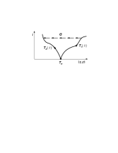
Figure 2: The Hamiltonian description of gauge transformations

If gauge transformations are given in terms of arbitrary parameters $\varepsilon(t)$ and their first time derivatives $\dot{\varepsilon}(t)$, as is the case with Poincaré gauge symmetry, the gauge generators have the form

$$G=\varepsilon(t)G_{0}+{\dot{\varepsilon}}(t)G_{1}\,,$$ (3.11a)

where phase space functions $$G_{0} G_{1}$$ and satisfy the conditions

and $C_{PFC}$ denotes primary FC constraint. These conditions clearly define the procedure for constructing the generator: one starts with an arbitrary primary FC constraint $G_{1}$, evaluates its PB with $H_{T}$, and defines $G_{0}$ in accordance with $\{G_{0},H_{T}\}=C_{PFC}$.

A detailed analysis, based on Castellani’s algorithm, shows that in all relevant physical applications Dirac’s conjecture remains true. This is of particular importance for the standard quantization methods, which are based on the assumption that all FC constraints are gauge generators.

Electrodynamics. Field theory can be thought of as a mechanical system in which dynamical variables are defined at each point $x$ of a three–dimensional space, $(q_{i},p_{i})\to(q_{ix},p_{ix})$ $\equiv(q_{i}(\hbox{\boldmath$x$}),p_{i}(\hbox{\boldmath$x$}))$, i.e. where each index takes on also continuous values, $i\equiv(i,\hbox{\boldmath$x$})$. Then, a formal generalization of the previous analysis to the case of field theory becomes rather direct.

We now discuss the simple but important example of electrodynamics, which is in many aspects similar to the theory of gravity. Dynamics of the free electromagnetic field $A^{\mu}(x)$ is described by the Lagrangian

$$L=-\hbox{${1\over 4}$}\int d^{3}xF_{\mu\nu}F^{\mu\nu}\,,\qquad F_{\mu\nu}=\partial_{\mu}A_{\nu}-\partial_{\nu}A_{\mu}\,.$$

Varying this Lagrangian with respect to $\dot{A}^{\mu}$ one obtains the momenta $\pi_{\mu}(x)=-F_{0\mu}(x)$, where $x\equiv(t,\hbox{\boldmath$x$})$. Since $F_{\mu\nu}$ is defined as the antisymmetric derivative of $A_{\mu}$, it does not depend on the velocity $\dot{A}^{0}$, so that the related momentum vanishes. Thus, one obtains the primary constraint $\varphi_{1}\equiv\pi_{0}\approx 0$, while $\pi_{\alpha}=-F_{0\alpha}$. With one primary constraint present, the total Hamiltonian takes the form

$$H_{T}=H_{c}+\int d^{3}xu(x)\pi_{0}(x)\,,$$

where $H_{c}=\int d^{3}x\bigl{(}\hbox{${1\over 4}$}F_{\alpha\beta}F^{\alpha\beta}-\hbox{${1\over 2}$}\pi_{\alpha}\pi^{\alpha}-A^{0}\partial^{\alpha}\pi_{\alpha}\bigr{)}$.

By use of the basic PBs, $\{A^{\mu}(x),\pi_{\nu}(x^{\prime})\}=\delta^{\mu}_{\nu}\delta(\hbox{\boldmath$x$}-\hbox{\boldmath$x$}^{\prime})$, the consistency condition for $\varphi_{1}$ leads to a secondary constraint: $\varphi_{2}\equiv\partial^{\alpha}\pi_{\alpha}\approx 0$. Further consistency requirement on $\varphi_{2}$ is automatically satisfied. The constraints $\varphi_{1}$ and $\varphi_{2}$ are FC, since $\{\pi_{0},\partial^{\alpha}\pi_{\alpha}\}=0$.

The variable $A^{0}$ appears linearly in $H_{c}$. Its equation of motion, $\dot{A}{{}^{0}}=\{A^{0},H_{T}\}=u$, implies that $A^{0}$ is also an arbitrary function of time. We observe that the secondary FC constraint $\varphi_{2}$ is already present in $H_{c}$ in the form $A^{0}\varphi_{2}$. In this way here, as well as in gravitation, we find an interesting situation that all FC constraints are present in $H_{T}$.

Let us now look for the generator of gauge symmetries in the form (3.11). Starting with $G_{1}=\pi_{0}$ one obtains

$$G=\int d^{3}x(\dot{\varepsilon}\pi_{0}-\varepsilon\partial^{\alpha}\pi_{\alpha})\,,$$

so that the related gauge transformations are $\delta_{0}A^{\mu}=\partial^{\mu}\varepsilon$, $\delta_{0}\pi_{\mu}=0$. The result has the form we know from the Lagrangian analysis.

The previous treatment fully respects the gauge symmetry of the theory. This symmetry can be fixed by choosing two gauge conditions. The dimension of the phase space $\Gamma(A,\pi)$ is eight; after fixing two gauge conditions we come to the phase space $\Gamma^{*}$ of dimension $N^{*}=8-2\times 2=4$, corresponding to two Lagrangian degrees of freedom of the massless photon.

4. Hamiltonian dynamics of PGT

PGT represents a natural extension of the gauge principle to spacetime symmetries. Now we want to present basic features of the Hamiltonian approach to the general PGT. It leads to a simple form of the gravitational Hamiltonian, representing a generalization of the canonical Arnowitt–Deser–Misner (ADM) Hamiltonian from GR [13], and enables a clear understanding of the interrelation between dynamical and geometric aspects of the theory [14, 15, 16].

Primary constraints. The geometric framework for PGT is defined by the Riemann–Cartan spacetime $U_{4}$, while the general Lagrangian has the form (2.4). The canonical momenta $(\pi_{k}{{}^{\mu}},\pi_{ij}{{}^{\mu}},\pi)$, corresponding to the basic Lagrangian variables $(b^{k}{{}_{\mu}},A^{ij}{{}_{\mu}},\psi)$, are obtained from $\widetilde{\cal L}$ in the usual manner.

Due to the fact that the curvature and the torsion are defined through the antisymmetric derivatives of $b^{k}{{}_{\mu}}$ and $A^{ij}{{}_{\mu}}$, respectively, they do not involve velocities of $b^{k}{{}_{0}}$ and $A^{ij}{{}_{0}}$. As a consequence, one immediately obtains the following set of the so–called sure primary constraints:

$$\phi_{k}{{}^{0}}\equiv\pi_{k}{{}^{0}}\approx 0\,,\qquad\phi_{ij}{{}^{0}}\equiv\pi_{ij}{{}^{0}}\approx 0\,.$$ (4.1)

These constraints are always present, independently of the values of parameters in the Lagrangian. They are particularly important for the structure of the theory. Depending on a specific form of the Lagrangian, one may also have additional primary constraints.

Hamiltonian. The canonical Hamiltonian has the form ${\cal H}_{c}={\cal H}_{M}+{\cal H}_{G}$, where ${\cal H}_{M}=\pi\partial_{0}\psi-\widetilde{\cal L}_{M}$, and ${\cal H}_{G}=\pi_{k}{{}^{\alpha}}\partial_{0}b^{k}{{}_{\alpha}}+\hbox{${1\over 2}$}\pi_{ij}{{}^{\alpha}}\partial_{0}A^{ij}{{}_{\alpha}}-\widetilde{\cal L}_{G}$. The total Hamiltonian is defined by the expression

$${\cal H}_{T}={\cal H}_{c}+u^{k}{{}_{0}}\phi_{k}{{}^{0}}+\hbox{${1\over 2}$}u^{ij}{{}_{0}}\phi_{ij}{{}^{0}}+(u\cdot\phi)\,,$$ (4.2)

where $\phi$ denotes all additional primary constraints if they exist (if–constraints).

The evaluation of the consistency conditions of the sure primary constraints (4.1) is essentially simplified if we previously find out the dependence of the Hamiltonian on the unphysical variables $b^{k}{{}_{0}}$ and $A^{ij}{{}_{0}}$. The analysis of this problem shows that ${\cal H}_{c}$ is linear in $b^{k}{{}_{0}}$ and $A^{ij}{{}_{0}}$, up to a three–divergence,

$${\cal H}_{c}=b^{k}{{}_{0}}{\cal H}_{k}-\hbox{${1\over 2}$}A^{ij}{{}_{0}}{\cal H}_{ij}+\partial_{\alpha}D^{\alpha}\,,$$ (4.3a)

while possible extra primary constraints $$\phi b^{k}{{}_{0}} A^{ij}{{}_{0}}$$ are independent of and .

The above result may be put into a more geometric form. If $n$ is the unit normal to the hypersurface $\Sigma_{0}:x^{0}=\hbox{const.}$, the four tangent vectors $(\hbox{\boldmath$n$},\hbox{\boldmath$e$}_{\alpha})$ define the so–called ADM basis. Any tangent vector $V_{k}$ can be expressed in terms of its orthogonal and parallel components: $V_{k}=n_{k}V_{\bot}+V_{{\bar{k}}}$, where $V_{\bot}=n^{k}V_{k}$, $V_{{\bar{k}}}=V_{k}-n_{k}V_{\bot}$, and $n^{k}V_{{\bar{k}}}=0$. With this notation, the above expression for ${\cal H}_{c}$ can be rewritten in an equivalent form:

$${\cal H}_{c}=N{\cal H}_{\bot}+N^{\alpha}{\cal H}_{\alpha}-\hbox{${1\over 2}$}A^{ij}{{}_{0}}{\cal H}_{ij}+\partial_{\alpha}D^{\alpha}\,,$$ (4.3b)

where $N$ and $N^{\alpha}$ are lapse and shift functions, which are linear in $b^{k}{{}_{0}}$: $N=n_{k}b^{k}{{}_{0}}$, $N^{\alpha}=h_{{\bar{k}}}{{}^{\alpha}}b^{k}{{}_{0}}$.

The proof of this relation for the matter Hamiltonian goes as follows. First, we decompose $\nabla_{k}\psi$ into its orthogonal and parallel components, $\nabla_{k}\psi=n_{k}\nabla_{\bot}\psi+\nabla_{{\bar{k}}}\psi$, where complete dependence on velocities and unphysical variables $(b^{k}{{}_{0}},A^{ij}{{}_{0}})$ is contained in $\nabla_{\bot}\psi$. Replacing this into ${\cal L}_{M}$ yields ${\cal L}_{M}={\bar{\cal L}}_{M}(\psi,\nabla_{{\bar{k}}}\psi,\nabla_{\bot}\psi;n^{k})$. Second, using the factorization of the determinant, $b=\det(b^{k}{{}_{\mu}})=NJ$, where $J$ does not depend on $b^{k}{{}_{0}}$, the expression for $\pi$ can be written in the form

$$\pi={\partial{\cal L}_{M}\over\partial\nabla_{0}\psi}=J{\partial\tilde{\cal L}_{M}\over\partial\nabla_{\bot}\psi}\,.$$

Finally, using the relation $\nabla_{0}\psi=N\nabla_{\bot}\psi+N^{\alpha}\nabla_{\alpha}\psi$ to express the velocity $\partial_{0}\psi$, the canonical Hamiltonian for matter fields takes the form (4.3b), where

Expressions for ${\cal H}^{M}_{\alpha}$ and ${\cal H}^{M}_{ij}$ are independent of unphysical variables. They do not depend on the specific form of the Lagrangian, but only on the transformation properties of the fields, and are called kinematical terms of the Hamiltonian. The term ${\cal H}_{\perp}^{M}$ is dynamical, as it depends on the choice of ${\cal L}_{M}$. It represents the Legendre transformation of ${\cal L}_{M}$ with respect to the “velocity” $\nabla_{\perp}\psi$. After eliminating $\nabla_{\perp}\psi$ with the help of the relation defining $\pi$, one finds that the dynamical Hamiltonian does not depend on unphysical variables: ${\cal H}_{\perp}^{M}={\cal H}_{\perp}^{M}(\psi,\nabla_{{\bar{k}}}\psi,\pi/J;n^{k})$.

If the matter Lagrangian is singular, the equations for momenta give rise to additional primary constraints, which are again independent of unphysical variables.

Construction of the gravitational Hamiltonian can be performed in a very similar way, the role of $\nabla_{k}\psi$ being taken over by $T^{i}{{}_{km}}$ and $R^{ij}{{}_{km}}$. In the first step we decompose the torsion and the curvature, in last two indices, in the orthogonal and parallel components. The parallel components $T^{i}{{}_{{\bar{k}}{\bar{m}}}}$ and $R^{ij}{{}_{{\bar{k}}{\bar{m}}}}$ are independent of velocities and unphysical variables. The replacement in the gravitational Lagrangian yields ${\cal L}_{G}={\bar{\cal L}}_{G}(T^{i}{{}_{{\bar{k}}{\bar{m}}}},R^{ij}{{}_{{\bar{k}}{\bar{m}}}},T^{i}{{}_{\bot{\bar{k}}}},R^{ij}{{}_{\bot{\bar{k}}}};n^{k})$. Using $b=NJ$ we find

$${\hat{\pi}}_{i}{{}^{{\bar{k}}}}=J{\partial{\bar{\cal L}}_{G}\over\partial T^{i}{{}_{\perp{\bar{k}}}}}\,,\qquad{\hat{\pi}}_{ij}{{}^{{\bar{k}}}}=J{\partial{\bar{\cal L}}_{G}\over\partial R^{ij}{{}_{\perp{\bar{k}}}}}\,,$$

where ${\hat{\pi}}_{i}{{}^{{\bar{k}}}}\equiv\pi_{i}{{}^{\alpha}}b^{k}{{}_{\alpha}}$ and ${\hat{\pi}}_{ij}{{}^{{\bar{k}}}}\equiv\pi_{ij}{{}^{\alpha}}b^{k}{{}_{\alpha}}$ are “parallel” gravitational momenta. The velocities $\partial_{0}b^{i}{{}_{\alpha}}$ and $\partial_{0}A^{ij}{{}_{\alpha}}$ can be calculated from the definitions of $T^{i}{{}_{0\alpha}}$ and $R^{ij}{{}_{0\alpha}}$. After a straightforward algebra the canonical Hamiltonian takes the form (4.3b), where

The expressions $T^{i}{{}_{\perp{\bar{m}}}}$ and $R^{ij}{{}_{\perp{\bar{m}}}}$ in ${\cal H}_{\perp}^{G}$ should be eliminated with the help of the equations defining ${\hat{\pi}}_{i}{{}^{{\bar{m}}}}$ and ${\hat{\pi}}_{ij}{{}^{{\bar{m}}}}$.

Secondary constraints. The basic result of the preceding exposition is the conclusion that the canonical Hamiltonian has the form (4.3b). Consequently, the consistency conditions of the sure primary constraints imply the following secondary constraints:

$${\cal H}_{\bot}\approx 0\,,\qquad{\cal H}_{\alpha}\approx 0\,,\qquad{\cal H}_{ij}\approx 0\,.$$ (4.6)

By working out the constraint algebra we shall see that the consistency conditions of these constraints are automatically satisfied.

Constraint algebra. When no extra constraints are present in the theory, the PB algebra of the secondary constraints (4.6) takes the form [17]

(4.7)

The first three relations represent PBs between kinematical constraints ${\cal H}_{ij}$ and ${\cal H}_{\alpha}$, the form of which does not depend of the choice of the action. The relations (LABEL:eq:4.7b) contain the dynamical part of the Hamiltonian ${\cal H}_{\bot}$.

Equations (4.7) in the local Lorentz basis take the form

featuring a visible analogy with the standard Poincaré algebra.

When extra constraints are present the whole analysis becomes much more involved, but the result essentially coincides with (4.7):

• dynamical Hamiltonian ${\cal H}_{\bot}$ goes over into a redefined expression ${\bar{\cal H}}_{\bot}$, that includes the contributions of all primary second class constraints;

• the algebra may contain terms of the type $C_{PFC}$.

Thus, secondary constraints (4.6) are FC, and their consistency conditions are automatically satisfied.

5. Gauge generators

The generators of the Poincaré gauge symmetry have the form $G=\dot{\varepsilon}(t)G^{(1)}+\varepsilon(t)G^{(0)}$, where $G^{(0)},G^{(1)}$ are phase space functions satisfying the conditions (LABEL:eq:3.11b). It is clear that the construction of the gauge generators demands the knowledge of the algebra of constraints. Since the Poincaré gauge symmetry is always present, independently of a specific form of the action, one naturally expects that all essential features of the Poincaré gauge generators can be obtained by considering the simple case of the theory with no extra constraints. After that, the obtained result is easily generalized [18].

When no extra constraints exist, the primary constraints $\pi_{k}{{}^{0}}$ and $\pi_{ij}{{}^{0}}$ are FC. Starting with $G_{k}^{(1)}=-\pi_{k}{{}^{0}}$, $G_{ij}^{(1)}=-\pi_{ij}{{}^{0}}$, and the related parameters $\xi^{k}$, $\varepsilon^{ij}$, the conditions (LABEL:eq:3.11b) yield the following expression for the Poincaré gauge generator :

$$G=-\int d^{3}x\bigl{[}\dot{\xi}^{\mu}\bigl{(}b^{k}{{}_{\mu}}\pi_{k}{{}^{0}}+\hbox{${1\over 2}$}A^{ij}{{}_{\mu}}\pi_{ij}{{}^{0}}\bigr{)}+\xi^{\mu}{\cal P}_{\mu}+\hbox{${1\over 2}$}\dot{\o}^{ij}\pi_{ij}{{}^{0}}+\hbox{${1\over 2}$}\o^{ij}S_{ij}\bigr{]}\,,$$ (5.1a)

where $$\xi^{\mu}=\xi^{k}h_{k}{{}^{\mu}} \o^{ij}=\varepsilon^{ij}+\xi^{\nu}A^{ij}{{}_{\nu}}$$ and are new parameters, and

Note that the time translation generator is equal to the total Hamiltonian, ${\cal P}_{0}=\hat{\cal H}{}_{T}\equiv{\cal H}_{T}-\partial_{\alpha}D^{\alpha}$, since $\dot{b}^{k}{{}_{0}}=u^{k}{{}_{0}}$, $\dot{A}^{ij}{{}_{0}}=u^{ij}{{}_{0}}$, on shell.

One can show that the action of the generator (5.1) on the fields $\psi,b^{k}{{}_{\mu}}$ and $A^{ij}{{}_{\mu}}$ produces the complete Poincaré gauge transformations:

where $\delta_{0}Q\equiv\{Q,G\}$. The only properties of the total Hamiltonian used in the derivation are the following: $a)$ ${\cal H}_{T}$ does not depend on the derivatives of momentum variables, and $b)$ it governs the time evolution of dynamical variables, i.e. $\dot{Q}=\{Q,H_{T}\}$.

In a similar way one can verify that the generator (5.1) produces the correct transformations of momenta.

We note here that the field transformations (LABEL:eq:5.2) are symmetry transformations of the action not only in the simple case characterized by the absence of any extra constraints, but also in the general case when these constraints exist. This fact leads to the conclusion that the gauge generator (5.1), in which the term $P_{0}$ is replaced by the new $\hat{\cal H}{}_{T}$, is the correct gauge generator of the Poincaré symmetry for any choice of parameters.

6. Conservation laws

Physical content of the notion of symmetry depends not only on the symmetry of the action, but also on the symmetry of boundary conditions. The choice of the asymptotic behaviour of gravitational variables defines the asymptotic structure of spacetime, i.e. the vacuum. The symmetry of the action breaks down to the symmetry of the vacuum (spontaneous symmetry breaking), which becomes the physical symmetry and determines the conservation laws. Thus, the possibility of defining the concept of energy (and other conserved quantities) depends essentially on the structure of asymptotic symmetries.

Assuming that the asymptotic symmetry in PGT is the global Poincaré symmetry, we discuss the form of the related generators. A careful analysis of boundary conditions leads to the appearance of certain surface terms in the expressions for the generators. The improved generators enable a correct treatment of the conservation laws of energy, momentum and angular momentum [19, 20].

Asymptotic symmetry. The global Poincaré transformations of fields in the asymptotic region can be obtained from the corresponding gauge transformations by the following replacement of parameters:

$$\o^{ij}(x)\to\o^{ij}\,,\qquad\xi^{\mu}(x)\to\o^{\mu}{{}_{\nu}}x^{\nu}+\varepsilon^{\nu}\equiv\xi^{\mu}\,,$$

where $\o^{ij}$ and $\varepsilon^{\nu}$ are constants. The generator of these transformations can be obtained from the gauge generator (5.1) in the same manner, leading to

$$G=\hbox{${1\over 2}$}\o^{ij}M_{ij}-\varepsilon^{\nu}P_{\nu}\,,$$ (6.1)

where

As the symmetry generators act on basic dynamical variables via PBs, they are required to have well defined functional derivatives. In case of parameters which decrease sufficiently fast at spatial infinity, all partial integrations in $G$ are characterized by vanishing surface terms, and the differentiability of $G$ does not represent any problem. The parameters of the global Poincaré symmetries are not of that type, so that surface terms must be treated more carefully. We shall try to improve the form of the generators (6.1) so as to obtain the expressions with well defined functional derivatives. The first step in that direction is to define precisely the phase space in which the generators (6.1) act.

The phase space. The choice of asymptotics becomes more clear if we express the asymptotic structure of spacetime in certain geometric terms. Here we shall consider isolated physical systems characterized by matter fields which decrease sufficiently fast at large distances, so that their contribution to surface integrals vanishes. The spacetime outside an isolated system is said to be asymptotically flat if the following two conditions are satisfied:

• $g_{\mu\nu}=\eta_{\mu\nu}+{\cal O}_{1}$, where ${\cal O}_{n}={\cal O}(r^{-n})$ denotes a term which decreases like $r^{-n}$ or faster for large $r$, and $r^{2}=(x^{1})^{2}+(x^{2})^{2}+(x^{3})^{2}$;

• $R^{ij}{{}_{\mu\nu}}={\cal O}_{2+\alpha}$ $(\alpha>0)$; this defines the absolute parallelism in the asymptotic region.

The second condition can be easily satisfied by demanding $A^{ij}{{}_{\mu}}={\cal O}_{1+\alpha}$. In the Einstein–Cartan (EC) theory, defined by the simple action $\sim\int d^{4}x\,bR$, the connection behaves as the derivative of the metric, i.e. $A={\cal O}_{2}$. We study here, for simplicity, the EC theory, i.e. we assume that the gravitational field behaves as

$$b^{k}{{}_{\mu}}=\delta^{k}_{\mu}+{\cal O}_{1}\,,\qquad A^{ij}{{}_{\mu}}={\cal O}_{2}\,.$$ (6.3)

In order to ensure the global Poincaré invariance of these conditions we demand $b^{k}{{}_{\mu,\nu}}={\cal O}_{2}$, $A^{ij}{{}_{\mu,\nu}}={\cal O}_{3}$, etc. The above requirements are minimal in the sense that some additional arguments may lead to a better asymptotics, i.e. to a faster or more precisely defined decrease of fields and their derivatives.

It should be noted that for those expressions that vanish on shell one can demand an arbitrarily fast asymptotic decrease, as no solutions of the field equations are thereby lost. In accordance with this, the asymptotic behavior of momenta is determined by requiring $p-{\partial{\cal L}/\partial{\dot{q}}}=\hat{\cal O}{}$, where $\hat{\cal O}{}$ denotes a term that decreases sufficiently fast. Using the definitions of the gravitational momenta in EC theory one finds [21]

$$\pi_{k}{{}^{0}},\pi_{ij}{{}^{0}}=\hat{\cal O}{}\,,\qquad\pi_{i}{{}^{\alpha}}=\hat{\cal O}{}\,,\qquad\pi_{ij}{{}^{\alpha}}=-4aJn_{[i}h_{j]}{{}^{\alpha}}+\hat{\cal O}{}\,,$$ (6.4)

where $\kappa\equiv 1/2a$ is Einstein’s gravitational constant. Similar arguments yield the consistent asymptotic behavior of the Hamiltonian multipliers.

Improving the Poincaré generators. The generators act on dynamical variables via the PB operation, which is defined in terms of functional derivatives. A functional $F[\varphi,\pi]=\int d^{3}xf\bigl{(}\varphi,\partial\varphi,\pi,\partial\pi\bigr{)}$ has well defined functional derivatives if its variation can be written in the form $\delta F=\int d^{3}x\bigl{[}A(x)\delta\varphi(x)+B(x)\delta\pi(x)\bigr{]}$, where terms $\delta\varphi_{,\mu}$ and $\delta\pi_{,\mu}$ are absent. The global Poincaré generators do not satisfy this requirement. However, this problematic behaviour can be simply corrected by adding certain surface terms.

Let us see how this procedure works in the case of global spatial translatios. The variation of $P_{\alpha}$ can be written in the form

$$\delta P_{\alpha}=-\delta E_{\alpha}+R\,,\qquad E_{\alpha}\equiv\oint ds_{\gamma}\bigl{(}\pi_{ij}{{}^{\beta}}A^{ij}{{}_{[\alpha}}\delta_{\beta]}{{}^{\gamma}}\bigr{)}\,,$$ (6.5a)

where $$R \delta\varphi_{,\mu} \delta\pi_{,\mu} E_{\alpha} P_{\alpha}$$ denotes regular terms, not containing , , and the integration domain in is the boundary of the three–dimensional space. After this we can redefine ,

$$P_{\alpha}\to\widetilde{P}_{\alpha}\equiv P_{\alpha}+E_{\alpha}\,,$$ (6.5b)

so that $\tilde{P}_{\alpha}$ has well defined functional derivative. One can check that the assumed asymptotic behavior of phase–space variables ensures finiteness of $E_{\alpha}$, which represents the value of linear momentum.

The improved expression for the time translation generator takes the form

$$\widetilde{P}_{0}=P_{0}+E_{0}\,,\qquad E_{0}\equiv\oint ds_{\gamma}(-2aJh_{a}{{}^{\alpha}}h_{b}{{}^{\gamma}}A^{ab}{{}_{\alpha}})\,.$$ (6.6)

The surface term $E_{0}$ is finite on account of the adopted asymptotics, and it represents the value of the energy of the system.

In a similar way we can improve the form of the spatial rotation and boost generators by introducing the following surface terms :

A detailed analysis shows that the adopted asymptotic conditions do not guarantee the finiteness of $E_{\alpha\beta}$, as the integrand contains ${\cal O}_{1}$ terms. These troublesome terms are seen to vanish if we impose the asymptotic gauge condition $a_{[ij]}={\cal O}_{2}$ on the gauge potentials $a^{k}{{}_{\mu}}=b^{k}{{}_{\mu}}-\delta^{k}_{\mu}$, and certain parity conditions. These conditions are invariant under the global Poincaré transformations, and they restrict the remaining gauge symmetry. After that the surface term $E_{\alpha\beta}$ is seen to be finite, and, consequently, $\widetilde{M}_{\alpha\beta}$ is well defined.

All these results are obtained in the EC theory. Analogous considerations in the general PGT show that the boost generator cannot be redefined by adding a surface term. Therefore, it is not a well defined generator under the adopted boundary conditions, but a refinement of these could, in principle, lead to a correctly defined boost generator.

Conservation laws. The improved generators satisfy the standard PB algebra, up to squares (or higher powers) of constraints and surface terms; this proves the asymptotic Poincaré invariance of the theory. We now wish to see whether this symmetry implies, as usual, the existence of certain conserved quantities.

After a slight modification Castellani’s method can be applied to study global symmetries, too. One can prove that necessary and sufficient conditions that a phase–space functional $G(q,\pi,t)$ should be a generator of global symmetries take the form

$$\{G,\widetilde{H}_{T}\}+{\partial G\over\partial t}=C_{PFC}\,,\qquad\{G,\varphi_{s}\}\approx 0\,,$$ (6.8)

where $\widetilde{H}_{T}$ is the improved Hamiltonian, $\varphi_{s}\approx 0$ are all constraints in the theory and, as before, the equality means an equality up to the zero generators.

The improved Poincaré generators are easily seen to satisfy the second condition, as they are given, up to surface terms, by volume integrals of FC constraints. The first condition represents the Hamiltonian form of the conservation law, since $dG/dt\equiv\{G,\widetilde{H}_{T}\}+\partial G/\partial t$. It can be used to explicitly check the conservation of $\widetilde{P}_{\mu}$ and $\widetilde{M}_{\mu\nu}$.

Let us begin with the energy. One can easily see that $d\widetilde{P}_{0}/dt=C_{PFC}$. Indeed, $\{\widetilde{P}_{0},\widetilde{P}_{0}\}=0$, and the only explicit time dependence is due to the presence of arbitrary multipliers, $\partial\widetilde{P}_{0}/\partial t=\int d^{3}x\dot{v}^{a}\varphi_{a}=C_{PFC}$. Hence,

$${d\widetilde{P}_{0}\over dt}\approx{dE_{0}\over dt}\approx 0\,,$$

and we see that $E_{0}$ represents the value of the energy as a conserved quantity.

The linear momentum $\widetilde{P}_{\alpha}$ and the spatial angular momentum $\widetilde{M}_{\alpha\beta}$ do not depend explicitly on time, and their conservation is verified in a similar manner. The boost generator has an explicit linear dependence on time, and ${d\widetilde{M}_{0\beta}/dt}\approx{dE_{0\beta}/dt}\approx-E_{\beta}$. Hence, since $E_{\beta}\neq 0$ in general, the boost generator is not a conserved quantity (it is conserved only in a reference frame where $E_{\beta}=0$). This is a consequence of an explicit linear time dependence of $\widetilde{M}_{0\beta}$, and the existence of a nonvanishing surface term in $\widetilde{P}_{\beta}$.

Comments. In order to compare these results with those obtained by the Lagrangian treatment, one should express all momentum variables in $E_{\mu}$ and $E_{\mu\nu}$ in terms of fields and their derivatives, with the help of the constraints and the equations of motion. A direct calculation shows that the energy–momentum and angular momentum in EC theory coincide with the related GR expressions.

In the general $R+T^{2}+R^{2}$ theory one obtains the same results only when all tordions ($A$–fields) are massive. The existence of massless tordions has the following consequences: $a)$ the spatial angular momentum $E_{\alpha\beta}$ becomes different from the GR expression, and $b)$ the boost $E_{0\beta}$ is not even defined in that case. The fact that the boost generator is always defined in the Lagrangian approach can be understood by observing that there one does not take care of the existence of functional derivatives of the symmetry generators.

7. The teleparallel form of GR

General geometric arena of PGT, the Riemann–Cartan space $U_{4}$, may be a priori restricted by imposing certain conditions on the curvature and the torsion. An interesting limit of PGT is teleparallel or Weitzenböck geometry $T_{4}$, defined by the requirement

$$R^{ij}{}_{\mu\nu}(A)=0\,.$$ (7.1)

The parallel transport in $T_{4}$ is path independent, i.e. we have an absolute parallelism. The teleparallel geometry is, in a sense, complementary to Riemannian geometry: while the curvature vanishes, the connection may have torsion (Figure 1). Of particular importance for the physical interpretation of this geometry is the fact that there is a one–parameter family of teleparallel Lagrangians which is empirically equivalent to GR [5, 22]. For the parameter value $B=1/2$ the Lagrangian of the theory coincides, modulo a four–divergence, with the Einstein–Hilbert Lagrangian, and defines the teleparallel form of GR, GR_∥.

The teleparallel description of gravity has been one of the most promising alternatives to GR. However, analyzing this theory Kopczyńsky [23] found a hidden gauge symmetry, and concluded that the torsion evolution is not completely determined by the field equations. Assuming, then, that the torsion should be a measurable physical quantity, he argued that this theory is internally inconsistent (see also Refs. [24] and [25]). Here we focus our attention on GR_∥, showing how Dirac’s canonical approach leads to a clear explanation of this, somewhat mysterious behaviour [26].

Lagrangian. Gravitational dynamics in the framework of the teleparallel geometry in PGT is described by a class of Lagrangians quadratic in the torsion [5, 22]

$$\halign to=0.0pt{\hfil\global\@eqcnt\z@$\displaystyle{#}$&\global\@eqcnt\@ne\hfil$\displaystyle{{}#{}}$\hfil&\global\@eqcnt\tw@$\displaystyle{#}$\hfil&\llap{#}\cr&&\tilde{\cal L}= b\bigl{(}{\cal L}_{T} +{\cal L}_{M}\bigr{)} + \l_{ij}{}^{\mu\nu}R^{ij}{}_{\mu\nu}\, ,\\ &\hbox to0.0pt{\hss&{\cal L}_{T}=a\bigl{(}AT_{ijk}T^{ijk}+BT_{ijk}T^{jik}+CT_{k}T^{k}\bigr{)}\equiv\beta_{ijk}(T)T^{ijk}\,,\cr}}$$

where the Lagrange multipliers $\l_{ij}{}^{\mu\nu}$ ensure the teleparallelism condition (7.1), $a=1/2\kappa$, $T_{k}=T^{m}{}_{mk}$, and ${\cal L}_{M}$ is the Lagrangian of matter fields. Note that, here, $\l_{ij}{}^{\mu\nu}$ is assumed to be a tensor density rather then a tensor, which simplifies the constraint analysis [26].

If we require that the theory (7. The teleparallel form of GR) describes all the standard gravitational tests correctly, we can restrict our considerations to the one–parameter family of Lagrangians, defined by the conditions $(i)$ $\,2A+B+C=0\,,C=-1$ [5, 22]. This family represents a viable gravitational theory for macroscopic, spinless matter, empirically indistinguishable from GR. Von der Heyde [27] and Hehl [5] have given certain theoretical arguments in favor of the choice $B=0$. There is, however, another, particularly interesting choice determined by the requirement $(ii)$ $\,2A-B=0$. It leads effectively to the Einstein–Hilbert Lagrangian ${\cal L}_{GR}=-abR(\Delta)$, defined in Riemann spacetime $V_{4}$ with Levi–Cività connection $A=\Delta$, via the geometric identity:

$$bR(A)=bR(\Delta)+b\bigl{(}\hbox{${1\over 4}$}T_{ijk}T^{ijk}+\hbox{${1\over 2}$}T_{ijk}T^{jik}-T_{k}T^{k}\bigr{)}-2\partial_{\nu}(bT^{\nu})\,.$$

Indeed, in Weitzenböck spacetime the above identity in conjunction with the condition (7.1) implies that the torsion Lagrangian (7. The teleparallel form of GR) is equivalent to the Einstein–Hilbert Lagrangian, up to a four–divergence, provided that

$$A=\hbox{${1\over 4}$}\,,\qquad B=\hbox{${1\over 2}$}\,,\qquad C=-1\,,$$ (7.3)

which coincides with the above conditions $(i)$ and $(ii)$.

The theory defined by Eqs. (7. The teleparallel form of GR) and (7.3) is called the teleparallel formulation of GR (GR_∥). It is equivalent to GR for scalar matter, but the gravitational couplings to spinning matter fields in $T_{4}$ and $V_{4}$ are in general different. In what follows we shall investigate the Hamiltonian structure and gauge properties of GR_∥ without matter fields, but the results obtained here will be also useful for the analysis of interacting theory.

Primary constraints. We begin the canonical analysis by observing the presence of the primary constraints (4.1). Similarly, the absence of the time derivative of $\l_{ij}{}^{\mu\nu}$ implies

$$\phi^{ij}{}_{\mu\nu}\equiv\pi^{ij}{}_{\mu\nu}\approx 0\,.$$ (7.4)

The next set of constraints follows from the linearity of the curvature in $\dot{A}^{ij}{}_{\alpha}$:

$$\phi_{ij}{}^{\alpha}\equiv\pi_{ij}{}^{\alpha}-4\l_{ij}{}^{0\alpha}\approx 0\,.$$ (7.5)

The system of equations defining ${\hat{\pi}}_{i{\bar{k}}}=\pi_{i}{{}^{\alpha}}b_{k\alpha}$ can be decomposed into irreducible parts with respect to the group of three–dimensional rotations in $\Sigma_{0}$. Taking into account the special choice of parameters adopted in equation (7.3), we obtain two sets of relations: the first set represents extra primary constraints (if–constraints),

$${\hat{\pi}}_{\perp{\bar{k}}}/J+2aT^{\bar{m}}{}_{{\bar{m}}{\bar{k}}}\approx 0\,,\qquad{\hat{\pi}}_{[{\bar{i}}{\bar{k}}]}/J-aT_{\perp{\bar{i}}{\bar{k}}}\approx 0\,,$$ (7.6a)

while the second set gives nonsingular equations, which can be solved for velocities. Further calculations are greatly simplified by observing that the set of extra constraints can be represented in a unified manner as

$$\phi_{ik}={\hat{\pi}}_{i{\bar{k}}}-{\hat{\pi}}_{k{\bar{i}}}+a\nabla_{\alpha}B^{0\alpha}_{ik}\,,\qquad B^{0\alpha}_{ik}\equiv\varepsilon^{0\alpha\beta\gamma}\varepsilon_{ikmn}b^{m}_{\beta}b^{n}_{\gamma}\,.$$ (7.6b)

Hamiltonian. Having found all the primary constraints, we can now calculate the canonical Hamiltonian density. Following the usual prescription [26] we obtain

(7.7)

where

$$D^{\alpha} \bar{T}_{ijk}=T_{i{\bar{j}}{\bar{k}}}$$ is the same as in Eq.(LABEL:eq:4.5), , and

Note minor changes in these expressions as compared to Eqs.(4.3b) and (LABEL:eq:4.5), which are caused by the presence of the Lagrange multipliers in Eq.(7. The teleparallel form of GR). The canonical Hamiltonian is now linear in unphysical variables $b^{k}{{}_{0}},A^{ij}{{}_{0}}$ and $\l_{ij}{}^{\alpha\beta}$.

The general Hamiltonian dynamics is described by the total Hamiltonian:

$${\cal H}_{T}={\cal H}_{c}+u^{i}{{}_{0}}\pi_{i}{{}^{0}}+\hbox{${1\over 2}$}u^{ij}{{}_{0}}\pi_{ij}{{}^{0}}+\hbox{${1\over 4}$}u_{ij}{}^{\mu\nu}\pi^{ij}{}_{\mu\nu}\\+\hbox{${1\over 2}$}u^{ik}\phi_{ik}+\hbox{${1\over 2}$}u^{ij}{{}_{\alpha}}\phi_{ij}{{}^{\alpha}}\,.$$

Although the torsion components $T_{\perp\perp{\bar{k}}}$ and $T^{A}_{{\bar{i}}\perp{\bar{k}}}$ are absent from the canonical Hamiltonian, they reappear in the total Hamiltonian as nondynamical multipliers. Indeed, the Hamiltonian field equations for $b^{k}{{}_{\alpha}}$ imply $NT_{\perp\perp{\bar{k}}}=u_{\perp{\bar{k}}}$, $NT^{A}_{{\bar{i}}\perp{\bar{k}}}=u_{{\bar{i}}{\bar{k}}}$. Thus, the existence of nondynamical torsion components is a phenomenon which is equivalent to the presence of extra FC constraints $\phi_{ik}$.

Consistency conditions. Having found the form of the primary constraints displayed in Eqs. (4.1), (7.4), (7.5) and (7.6), we now consider the requirements for their consistency.

The consistency conditions of the constraints (4.1) have the form (4.6). Similarly,

Since the equation of motion $\dot{A}^{ij}{{}_{\beta}}=\{A^{ij}{{}_{\alpha}},{\cal H}_{T}\}$ implies $R^{ij}{}_{0\beta}\approx u^{ij}{{}_{\beta}}$, all components of the curvature tensor weakly vanish, as one could have expected.

The consistency condition for $\phi_{ij}{}^{\alpha}$ can be used to determine $u_{ij}{}^{0\alpha}$:

where a bar over $u$ is used to denote the determined multiplier. Thus, the total Hamiltonian can be written in the form (7. The teleparallel form of GR) with $u^{ij}{{}_{\alpha}}=0$ and $u_{ij}{}^{0\alpha}\to\bar{u}_{ij}{}^{0\alpha}$. Since $\bar{u}_{ij}{}^{0\alpha}$ is linear in the multipliers $(N,N^{\alpha},A^{ij}{{}_{0}},\l_{ij}{}^{0\alpha},u_{kl})$, the total Hamiltonian takes the form

(7.10)

where

The consistency conditions for the tetrad constraints $\phi_{ij}$, technically the most complicated ones, are found to be automatically fulfilled: $\dot{\phi}_{ij}=\{\phi_{ij},{\cal H}_{T}\}\approx 0$.

Thus, the only secondary constraints are (4.1) and $R^{ij}{}_{\alpha\beta}\approx 0$. Their consistency conditions are found to be identically satisfied; hence there are no tertiary constraints.

Constraints and gauge symmetries. In the previous analysis we found that GR_∥ is characterized by the following set of constraints:

• primary:$\quad\pi_{i}{{}^{0}},\pi_{ij}{{}^{0}},\phi_{ij},\phi_{ij}{{}^{\alpha}},\pi^{ij}{}_{\alpha\beta},\pi^{ij}{}_{0\beta}\,$; secondary:$\quad{\cal H}_{\perp},{\cal H}_{\alpha},{\cal H}_{ij},\chi^{ij}{}_{\alpha\beta}$.

The essential dynamical classification of these constraints reads as follows:

• first class:$\quad\pi_{i}{{}^{0}},\pi_{ij}{{}^{0}},\pi^{ij}{}_{\alpha\beta},\bar{\phi}_{ij},{\bar{\cal H}}_{\perp},{\bar{\cal H}}_{\alpha},{\bar{\cal H}}_{ij},\bar{\chi}^{ij}{}_{\alpha\beta}\,$; second class:$\quad\phi_{ij}{{}^{\alpha}},\pi^{ij}{}_{0\beta}\,$.

The constraints $\phi_{ij}{{}^{\alpha}}$ and $\pi^{ij}{}_{0\beta}$ are second class since $\{\phi_{ij}{{}^{\alpha}},\pi^{kl}{}_{0\beta}\}\not\approx 0$. They can be used as strong equalities to eliminate $\l_{ij}{}^{0\alpha}$ and $\pi^{ij}{}_{0\beta}$ from the theory and simplify the exposition. The FC constraints are identified by observing that they appear multiplied by arbitrary multipliers in the total Hamiltonian (LABEL:eq:7.11a).

The algebra of FC constraints plays an important role not only in the construction of classical gauge generators, but also in studying quantum properties of GR_∥, such as the BRST structure. These important subjects deserve further investigation.

The complete set of gauge generators for GR_∥ can be constructed starting from the primary FC constraints $\pi_{i}{{}^{0}}$, $\pi_{ij}{{}^{0}}$, $\pi^{ij}{}_{\alpha\beta}$ and $\bar{\phi}_{ij}$. One should note that $\pi_{i}{{}^{0}}$, $\pi_{ij}{{}^{0}}$ and $\pi^{ij}{}_{\alpha\beta}$ are always present in the teleparallel geometry (7. The teleparallel form of GR), while $\bar{\phi}_{ij}$ are typical if–constraints. The role of $\pi_{i}{{}^{0}}$ and $\pi_{ij}{{}^{0}}$ in the Poincaré gauge symmetry is well known, but the meaning of gauge symmetries generated by $\pi^{ij}{}_{\alpha\beta}$ and $\bar{\phi}_{ij}$ is not completely clear [26]. The related gauge features of GR_∥ should be further analyzed.

The existence of extra FC constraints $\bar{\phi}_{ij}$ may be interpreted as a consequence of the fact that the velocities contained in $T_{\perp\perp{\bar{k}}}$ and $T^{A}_{{\bar{i}}\perp{\bar{k}}}$ appear at most linear in the Lagrangian and, consequently, remain arbitrary functions of time. Heht et al. [28] concluded that the initial–value problem for GR_∥ becomes well defined if these undetermined velocities are simply gauged away, ensuring the new kinetic Hessian matrix to be nondegenerate. However, this conclusion should not be taken as a definitive one before investigating possible nonlinear constraint effects [29, 25].

We note that Maluf [30] tried to analyze the canonical structure of GR_∥ by imposing the time gauge at the Lagrangian level. However, his arguments concerning the necessity of the time gauge are not acceptable: it is clear that this gauge may be useful, but certainly not essential. After fixing the time gauge, he found the Hamiltonian and derived the related set of constraints (which is not complete), but was unable to calculate the constraint algebra unless imposing another gauge condition. Thus, his analysis of the gauge structure of GR_∥ remaines rather unclear.

8. Concluding remarks

In this paper we presented basic features of the Hamiltonian structure of PGT using Dirac’s method for constrained dynamical systems.

1) We first gave a short review of PGT and Dirac’s method, by focussing our attention on those aspects that are essential for the analysis of the canonical structure of PGT.

2) The general form of the canonical PGT Hamiltonian is displayed in Eqs.(4.3). This important result shows that ${\cal H}_{c}$ is linear in unphysical variables $b^{k}{{}_{0}}$ and $A^{ij}{{}_{0}}$, whereupon one simply obtains the secondary constraints ${\cal H}_{\perp}\approx 0,{\cal H}_{\alpha}\approx 0$ and ${\cal H}_{ij}\approx 0$.

3) The PB algebra of the Hamiltonian constraints ${\cal H}_{\perp},{\cal H}_{\alpha}$ and ${\cal H}_{ij}$ is found to have the general form shown in Eq.(4.7). This result is essential for studying the canonical consistency of PGT.

4) The PB algebra of constraints is used to construct the general form of the generators of local Poincaré symmetry.

5) Assuming that spacetime behaves asymptotically as Minkowski space $M_{4}$, one obtains the corresponding global Poincaré generators. The surface terms related to the improved form of these generators are seen to represent the related conserved charges — energy, momentum and angular momentum.

6) The constrained Hamiltonian analysis of noninteracting GR_∥ is carried out without any gauge fixing, leading to the standard, consistent canonical behaviour (up to the question of possible nonlinear constraint effects). Extra gauge symmetries are found as a specific feature of GR_∥, and we are now investigating the conservation laws [31].

References

- [1] T. W. B. Kibble, Lorentz invariance and the gravitational field, J. Math. Phys. 2 (1961) 212; see also R. Utiyama, Invariant theoretical interpretation of interactions, Phys. Rev. 101 (1956) 1597.
- [2] F. W. Hehl, P. von der Heyde. D. Kerlick and J. Nester, General relativity with spin and torsion: Foundations and prospects, Rev. Mod. Phys. 48 (1976) 393.
- [3] F. W. Hehl, Four lectures in Poincaré gauge theory, in Cosmology and Gravitation: Spin, Torsion, Rotation and Supergravity, eds. P. G. Bergman and V. de Sabbata (Plenum, New York, 1980) p. 5.
- [4] K. Hayashi and T. Shirafuji, Gravity from the Poincaré gauge theory of fundamental interactions, I. General formulation, II. Equations of motion for test bodies and various limits, III. Weak field approximation, IV. Mass and energy of particle spectrum, Prog. Theor. Phys. 64 (1980) 866, 883, 1435, 2222.
- [5] F. W. Hehl, J. Nietsch and P. von der Heyde, Gravitation and the Poincaré gauge theory with quadratic Lagrangian, in General Relativity and Gravitation — One Hundred Years after the birth of Albert Einstein, ed. A. Held (Plenum, New York, 1980) vol. 1, p. 329.
- [6] M. Blagojević, Gravitation and gauge symmetries (submitted for publication). Chapters III, V and VI of this book give a systematic exposition of the Poincaré gauge theory, its canonical structure and conservation laws.
- [7] F. W. Hehl, J. D. McCrea, E. W. Mielke and Y. Ne’eman, Metric–affine gauge theory of gravity: field equations, Noether identities, world spinors and breaking of dilation invariance, Phys. Rep. C258 (1995) 1; F. Gronwald and F. W. Hehl, On the gauge aspects of gravity, Proc. of the 14th Course of the School on Cosmology and Gravitation on Quantum Gravity, held at Erice, Italy, 1995, P. G. Bergmann, V. de Sabata and H. J. Treder, eds. (World Scientific, Singapore, 1996).
- [8] Y. Choquet–Bruhat, C. De Witt–Morette and M. Dilard–Bleik, Analysys, manifolds and physics (North Holland, Amsterdam, 1977).
- [9] P. von der Hayde, The equivalence principle in the theory of gravitation, Nouvo Cim. Lett. 14 (1975) 250.
- [10] P. A. M. Dirac, Lectures on Quantum Mechanics (New York, Yeshiva University, 1964); A. Hanson, T. Regge and C. Teitelboim, Constrained Hamiltonian Dynamics (Rome, Academia Nacionale dei Lincei, 1976); K. Sundermeyer, Constrained Dynamics (Berlin, Springer, 1982); D. M. Gitman and I. V. Tyutin, Kanonicheskoe Kvantovanie Polei so Svyazami (Nauka, Moskva, 1986).
- [11] M. Henneaux and C. Teitelboim, Quantization of gauge systems (Princeton University Press, Princeton, 1992);
- [12] L. Castellani, Symmetries and constrained Hamiltonian systems, Ann. Phys. (N.Y.) 143 (1982) 357.
- [13] R. Arnowit, S. Deser and C. W. Misner, The dynamics of general relativity, in Gravitation — an Introduction to Current Research, ed. L. Witten (Wiley, New York), p. 227.
- [14] I. A. Nikolić, Dirac Hamiltonian structure of Poincaré gauge theory of gravity without gauge fixing, Phys. Rev. D30 (1984) 2508; M. Blagojević and I. A. Nikolić, Hamiltonian dynamics of Poincaré gauge theory: General structure in the time gauge, Phys. Rev. D28 (1983) 2455;
- [15] J. M. Nester, Some Progress in Classical Canonical Gravity, in Directions in general relativity, Proc. of the 1993 International symposium, Maryland, vol. I, papers in honour of Charles Misner, edited by B. L. Hu, M. P. Ryan and C. V. Vishveshwara (Cambridge University Press, Cambridge 1993) p. 245. This paper gives a review of the covariant Hamiltonian approach based on differential form methods.
- [16] M. Blagojević, Conservation laws in Poincaré gauge theory, Acta Phys. Pol. B29 (1998) 881.
- [17] I. A. Nikolić, Canonical structure of Poincaré gauge–invariant theory of gravity, Fiz. Suppl. 1 (1986) 135; M. Blagojević and M. Vasilić, Constraint algebra in Poincaré gauge theory, Phys. Rev. D36 (1987) 1679; I. A. Nikolić, Constraint algebra from local Poincaré symmetry, Gen. Rel. Grav. 24 (1992) 159.
- [18] M. Blagojević, I. Nikolić and M. Vasilić, Local Poincaré generators in the theory of gravity, Il Nuovo Cim. 101B (1988) 439.
- [19] T. Regge and C. Teitelboim, Role of surface integrals in the Hamiltonian formulation of general relativity, Ann. Phys. (N.Y.) 88 (1974) 286.
- [20] M. Blagojević and M. Vasilić, Assymptotic symmetries and conservation laws in the Poincaré gauge theory, Class. Quant. Grav. 5 (1988) 1241.
- [21] I. A. Nikolić, Dirac Hamiltonian formulation and algebra of the constraints in the Einstein–Cartan theory, Class. Quant. Grav. 12 (1995) 3103.
- [22] K. Hayashi and T. Shirafuji, New general relativity, Phys. Rev. D19 (1979) 3524; J. Nitsch, The macroscopic limit of the Poincaré gauge theory of gravitation, in Cosmology and Gravitation: Spin, Torsion, Rotation and Supergravity, eds. P. G. Bergman and V. de Sabbata (Plenum, New York, 1980) p. 63.
- [23] W. Kopczyński, Problems with metric–teleparallel theories of gravitation, J. Phys. A15 (1982) 493.
- [24] J. Nester, Is there really a problem with the teleparallel theory?, Class. Quant. Grav. 5 (1988) 1003.
- [25] Wen–Hao Cheng, De–Ching Chern and James M. Nester, Canonical analysis of the one–parameter teleparallel theory, Phys. Rev. D38 (1988) 2656.
- [26] M. Blagojević and I. A. Nikolić, Hamiltonian structure of the teleparallel formulation of general relativity, Phys. Rev. D (to be published), hep-th/0002022.
- [27] P. von der Heyde, The field equations of the Poincaré gauge theory of gravitation, Phys. Lett. 58A (1976) 141; Is gravitation mediated by the torsion of spacetime?, Z. Naturf. 31a (1976) 1725.
- [28] R. D. Hecht, J. Lemke and R. P. Walner, Can Poincaré gauge theory be saved?, Phys. Rev. D44 (1991) 2442.
- [29] Hsin Chen, James M. Nester and Hwei–Jang Yo, Acausal PGT modes and the nonlinear constraint effect, Acta Phys. Pol. B29 (1998) 961.
- [30] J. W. Maluf, Hamiltonian formulation of the telepaerallel description of general relativity, J. Math. Phys. 35 (1994) 335.
- [31] M. Blagojević and M. Vasilić, in preparation.