TPI-MINN-00/27-T

UMN-TH-1908/00

FTUV/000601

IFIC/00-32

Leaving the BPS bound: Tunneling of classically saturated solitons

D. Binosi

Departamento de Física Teórica and IFIC, Centro Mixto,
Universidad de Valencia-CSIC,
E-46100, Burjassot, Valencia, Spain

M. Shifman and T. ter Veldhuis

Theoretical Physics Institute, Univ. of Minnesota, Minneapolis, MN 55455

We discuss quantum tunneling between classically BPS saturated solitons in two-dimensional theories with ${\cal N}=2$ supersymmetry and a compact space dimension. Genuine BPS states form shortened multiplets of dimension two. In the models we consider there are two degenerate shortened multiplets at the classical level, but there is no obstruction to pairing up through quantum tunneling. The tunneling amplitude in the imaginary time is described by instantons. We find that the instanton is nothing but the $1/4$ BPS saturated “wall junction,” considered previously in the literature in other contexts. Two central charges of the superalgebra allow us to calculate the instanton action without finding the explicit solution (it is checked, though, numerically, that the saturated solution does exist). We present a quantum-mechanical interpretation of the soliton tunneling.

E-mail: binosi@titan.ific.uv.es, shifman@physics.spa.umn.edu, veldhuis@hep.umn.edu

1 Introduction

Bogomol’nyi-Prasad-Sommerfield (BPS) saturated topologically stable solitons in supersymmetric theories are widely discussed at present in connection with the brane world scenarios [1, 2]. In theories with compact spatial dimension(s), two distinct degenerate mass solitons which are BPS saturated classically, and to any finite order in perturbation theory, can mix nonperturbatively, thus lifting the BPS bound. Two shortened supermultiplets pair up with each other combining in one full supermultiplet with mass $M>|Z|$, where $Z$ is the central charge of the superalgebra. This phenomenon is an analog (in the soliton sector) of the spontaneous breaking of supersymmetry due to instantons in the vacuum sector [3, 4]. To the best of our knowledge it was first considered in the context of ${\cal N}=2$ two-dimensional Wess-Zumino models in [5].

In this work we address the issue of calculating the shift $M-|Z|$. In the quasi-classical approximation, it is proportional to the tunneling probability which, in turn, is determined by instantons. Remarkably, the instanton calculus in this case is nothing but an adaptation of the theory of the BPS saturated wall junctions, which also received much attention recently [6, 7, 8, 9, 10, 11, 12]. In particular, the instanton action can be derived from the central charges. The explicit formula for the instanton solution is not needed. The only thing we need to know is the very fact of its existence. This is in perfect parallel with the standard (non-supersymmetric) instantons: once one knows that the self-duality equations have a solution, the instanton action is unambiguously fixed in terms of the topological charge.

In Ref. [5] it was observed that the soliton mixing, resulting in the loss of the BPS saturation, can be described by an effective SUSY quantum mechanics; however, the general construction presented there, is not very transparent. Here we reduce the construction of Ref. [5] to a simple limiting case which nicely illustrates the essence of the phenomenon.

The organization of the paper is as follows. In Section 2 we formulate the problem and elaborate general aspects of the solutions. In Section 3 a specific instructive example is considered. Section 4 is devoted to SUSY quantum mechanics.

2 Formulation of the problem and general results

Classically BPS saturated soliton supermultiplets which may become degenerate in mass with some other supermultiplets and lift the BPS bound because of a nonperturbative mixing, is a rather general feature of various theories. Although our results are applicable in all cases, we find it convenient to explain the problem in a specific setting.

Consider a two-dimensional ${\cal N}=2$ Wess-Zumino model of one chiral superfield $\Phi$ with the superpotential ${\cal W}(\Phi)$. Any model of this type can be obtained as a two-dimensional reduction of the corresponding four-dimensional theory. The geometry of the world sheet is a cylinder. As explained in [5], for the existence of the BPS solitons it is necessary that ${\cal W}(\Phi)$ is a multi-branch function (otherwise the vanishing of the central charge $Z$ cannot be avoided), while $d{\cal W}/d\Phi$ must be meromorphic. Another necessary (and sufficient) condition for the topologically stable solitons is the existence of non contractable cycles in the target space. One of the simplest choices is a target space with the topology of a cylinder, possibly with punctured points. Then the periods of $\cal W$ are the central charges of the SUSY algebra,

$$Z_{i}=2\oint_{{\rm nc}_{i}}d{\cal W},$$ (1)

where nc_i stands for the $i$-th non-contractable contour in the target space.

Figure 1: a) The general singularity structure of the quantity $d{\mathcal{W}}/d\Phi$ in the complex $\Phi$ plane; b) the critical trajectories corresponding to infinite periods.

If there is at least one non-contractable cycle, one can always define $\Phi$ in such a way that $d{\cal W}$ is periodic

$$d{\cal W}(\Phi+2\pi)=d{\cal W}(\Phi).$$ (2)

This particular parametrization is not crucial, and is imposed only for the purpose of making the presentation simpler. The poles of $d{\cal W}/d\Phi$ are assumed to be single poles; quadratic and higher order poles can be treated as a limiting case of coinciding single poles. A generic singularity structure of $d{\cal W}/d\Phi$ is depicted in Fig. 1a), where the poles are marked by bold dots. The Kähler potential is taken to be trivial, ${\cal K}(\Phi,\bar{\Phi})=\Phi\bar{\Phi}$.

Consider the cycle $\Gamma_{1}$, for which

$$Z_{1}=2\int_{\Gamma_{1}}\!d\Phi\left(\frac{d{\cal W}}{d\Phi}\right).$$ (3)

If $Z_{1}=|Z_{1}|e^{\imath\delta}$, then the equation for the static BPS soliton has the form

$$\frac{d\Phi}{dx}=e^{\imath\delta}\frac{d\bar{\cal W}}{d\bar{\Phi}}.$$ (4)

This equation admits the “integral of motion”,

$$I={\rm Im}\left(e^{-\imath\delta}{\cal W}\right),$$ (5)

i.e. $dI/dx=0$ when $\cal W$ and $\bar{\cal W}$ are evaluated on the solution of (4). The existence of this integral of motion allows one to find the BPS solution in the general case [5]. The strategy is as follows. We first ignore that the world sheet is a cylinder with period $L$ in the $\hat{x}$ direction, and solve the BPS equation without posing the condition of periodicity, $\Phi(x+L)=\Phi(x)$. The solution found in this way is marked by the continuous (real) parameter $I$, and is a periodic function of $x$ with period

$$\ell(I)=\int d\Phi\left(e^{\imath\delta}\frac{d\bar{\cal W}}{d\bar{\Phi}}\right)_{\bar{\Phi}=\bar{\Phi}_{I}(x)}^{-1}.$$ (6)

The period function $\ell(I)$ is real and positive. It is not difficult to show that there exist critical values of $I$ such that $\ell(I)\rightarrow\infty$ at $I\downarrow I_{*l}$ or $I\uparrow I_{*r}$, where $I_{*l,r}$ mark the critical trajectories running close to the nearest poles of $\cal W$ from the left and from the right (Fig. 1b). A schematic plot of the function $\ell(I)$ is presented in Fig. 2.

Figure 2: The period function $\ell$ versus $I$.

If the circumference of the worldsheet cylinder $L>\ell_{\mathrm{min}}$, then the equation $\ell(I)=L$ has an even number of solutions. The corresponding values $I_{i}$ belongs to the interval $(I_{*l},I_{*r})$, while $\Phi_{I_{i}}(x)$, $i=1,2,...,2\nu$ are the classical BPS solutions satisfying Eq. (4) and the periodicity condition $\Phi_{I_{i}}(x+L)=\Phi_{I_{i}}(x)$.

In the case at hand they have particle interpretation. Altogether, we have $2\nu$ supermultiplets, each containing two states. All masses are degenerate and equal to $|Z_{1}|$.

The BPS nature of the solitons established above at the classical level persists to any finite order in perturbation theory (this statement assumes that there is a small expansion parameter in the superpotential and/or the Kähler function). Alternatively, one can say that $2\nu$ BPS solitons remain under small deformations of the parameters. This is due to the fact that the number of states in the supermultiplet is two, while the full ${\cal N}=2$ supermultiplet contains four states. The BPS supermultiplets are shortened.

It is equally clear, however, that nonperturbatively the BPS saturation of the solitons under consideration is lifted, they pair up to form $\nu$ full supermultiplets which lift the BPS bound. This was noted in [5], where arguments were given based on the Cecotti-Vafa-Intriligator-Fendly (CVIF) index [13]. Our task here is to calculate $M-|Z_{1}|$ in the quasi-classical approximation (which implies of course that $(M-|Z_{1}|)/|Z_{1}|\ll 1$).

The BPS saturation is lifted by tunneling. Consider for simplicity the case when Eq. (4) has only two solutions, $\Phi_{I_{1}}(x)\equiv\phi_{1}(x)$ and $\Phi_{I_{2}}(x)\equiv\phi_{2}(x)$. One can construct an interpolating field configuration $\phi(t,x)$ (where $t$ is the Euclidean time) such that in the distant past

$$\phi(t,x)\,{\buildrel t=-T/2\to-\infty\over{\hbox to60.0pt{\rightarrowfill}}}\,\phi_{1}(x),$$ (7)

and in the distant future

$$\phi(t,x)\,{\buildrel t=T/2\to\infty\over{\hbox to60.0pt{\rightarrowfill}}}\,\phi_{2}(x),$$ (8)

The interpolation is smooth (in particular, $\phi(t,x+L)=\phi(t,x)$ for all $t$), so that the (Euclidean) action $A$

$$A\left[\phi(t,x)\right]-|Z|T$$ (9)

is finite. Here $|Z|$ is the soliton mass in the absence of the tunneling. The quasi-classical formalism is applicable provided $A-|Z|T\gg 1$. One must minimize over all interpolating trajectories; once the trajectory $\phi_{0}(t,x)$ corresponding to the minimal action is found, one can calculate

$$\Delta A_{\rm min}=A\left[\phi_{0}(t,x)\right]-|Z|T.$$ (10)

The shift of the soliton masses from the BPS bound is then

$$\Delta M=M-|Z|\propto e^{-2\Delta A_{\rm min}},$$ (11)

where the factor of $2$ in the exponent is due to the fermion zero modes. We will comment more on this factor in Section 4.

The central result of the present work is as follows. The determination of the minimizing trajectory $\phi_{0}(t,x)$ (in the Euclidean time) reduces to the problem of determining the BPS wall junction in the $(1+2)$-dimensional theory, in which the $(1+1)$-dimensional model under consideration is embedded. The embedding is trivial. Indeed, if the original model is a $(1+1)$-dimensional slice of the four dimensional Wess-Zumino model, the one in which we embed is a $(1+2)$-dimensional slice of the very same model. From this remark it is clear that the formalism we discuss is applicable, generally speaking, in the supersymmetric theories with extended supersymmetry (${\cal N}=2$ or ${\cal N}=4$). In fact, since the solitons – the “walls” and “wall junctions” – are static, we will have to deal with one- and two-dimensional problems, respectively.

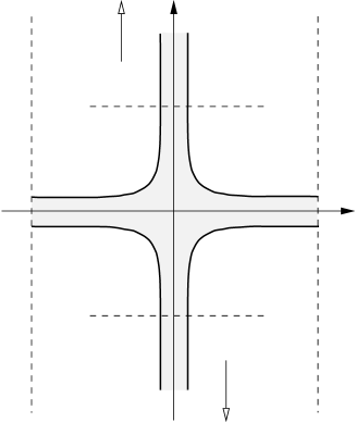
Figure 3: The energy distribution corresponding to the interpolating configuration; the unshaded area has the “vacuum” energy density.

The energy distribution for the interpolating configuration $\phi_{0}(t,x)$ is schematically depicted in Fig. 3. It is nothing but an adaptation of the standard four-wall junction on the cylinder world sheet. The equation for the BPS wall junction has the form

$$\frac{\partial\phi}{\partial\zeta}=\frac{1}{2}\frac{d\bar{\mathcal{W}}}{d\bar{\phi}},$$ (12)

where $\zeta$ is the complex variable $\zeta=x+it$, and $\partial_{\zeta}=1/2(\partial_{x}-\imath\partial_{t})$. The solution to this equation, if it exists, is $1/4$ BPS saturated. Equation (12) was first derived in [14]. The fact that the solution of Eq. (12) minimizes the Euclidean action is quite obvious. Indeed,

$$A = \int dt\,dx\,\left(\left|\frac{\partial\phi}{\partial t}\right|^{2}+\left|\frac{\partial\phi}{\partial x}\right|^{2}+\left|\frac{d{\cal W}}{d\phi}\right|^{2}\right),$$

$$= \int dt\,dx\,\,\left(2\frac{\partial\phi}{\partial\zeta}-\frac{d\bar{\cal W}}{d\bar{\phi}}\right)\left(2\frac{\partial\bar{\phi}}{\partial\bar{\zeta}}-\frac{d{\cal W}}{d\phi}\right)+\,\,{\rm surface}\,\,\,{\rm terms}.$$

The surface terms are unambiguously fixed by the boundary conditions, Eqs. (7) and (8), and by the periodicity condition $\phi(t,x+L)=\phi(t,x)$. Thus, the construction is quite analogous to the instanton self-duality equation in the Yang-Mills theory or the two-dimensional $O(3)$ sigma model, where the surface terms are topological charges.

In the supersymmetric model under consideration the surface terms are proportional to two distinct central charges which exist in the superalgebra [10]. One central charge is related to the junction “spokes”. In fact, this was discussed above, see Eq. (1). Another central charge is related to the junction “hub”.

In what follows we will assume the circumference of the world sheet cylinder to be large. This is sufficient to ensure the applicability of the quasi-classical approximation.

In the quasi-classical limit $L\rightarrow\infty$ the central charge related to the junction is subdominant. From Fig. 3, it is evident that at $L\rightarrow\infty$ the minimal action is

$$\Delta A_{\rm min}=L\sigma,$$ (14)

where $\sigma$ is the tension of the horizontal “wall”,

$$\sigma=2(I_{*r}-I_{*l}).$$ (15)

The effect of the “hub” is subdominant, it is proportional to $L^{0}$, and may be of the same order as the pre-exponential factors due to the zero modes. Thus,

$$M-|Z|\propto e^{-4(I_{*r}-I_{*l})L}.$$ (16)

In the next section we will consider a concrete model, which seems to present an instructive example. In this particular model we calculate for $\Delta A_{\rm min}$ both the linear term in $L$ and, for the sake of completeness, the next to leading term associated with the $(1/2,1/2)$ central charge, the “hub”.

The remainder of the paper presents an illustration and elaboration of the above general results.

3 An (instructive) example

In this section we apply the previous considerations to a specific model which was first introduced in [5]. We consider a generalized Wess-Zumino model for which

$${\mathcal{K}}(\Phi,\bar{\Phi})=\Phi\bar{\Phi},\qquad d{\mathcal{W}}=\frac{4\pi}{2-\cos\Phi}d\Phi,$$ (17)

where $d{\mathcal{W}}/d\Phi$ is a single-valued function derived from the multi-valued superpotential

$${\mathcal{W}}=\frac{8\pi}{\sqrt{3}}\arctan\left(\sqrt{3}\tan\frac{\Phi}{2}\right).$$ (18)

The model possesses only a run-away vacuum $|{\mathrm{Im}}(\phi)|\to\infty$. It is stabilized by solitons, which at the classical level are solutions to the BPS equation given by Eq. (4).

The target space has the topology of a cylinder ($-\infty<{\mathrm{Im}}(\phi)<+\infty,\ -\pi\leq{\mathrm{Re}}(\phi)\leq\pi$), with the poles of the scalar potential,

$$(\phi_{*})_{1,2}=\pm\imath\log\left(2+\sqrt{3}\right),$$ (19)

removed. Each soliton solution belongs to one of three homotopy classes, $\Gamma_{1}$, $\Gamma_{2}$ and $\Gamma_{3}$. Solutions in $\Gamma_{1}$ wind around the target space cylinder, whereas solutions in $\Gamma_{2}$ and $\Gamma_{3}$ wind around the points that are removed from the target space (see Fig. 4). Each solution in $\Gamma_{1}$ has a mirror image in the real axis of the complex $\phi$ plane that belongs to the same class, except for a real soliton, which is invariant under this transformation. Solutions in $\Gamma_{2}$ are mapped to solutions in $\Gamma_{3}$ and vice versa. The solutions in all homotopy classes have equal period,

$$\Delta{\mathcal{W}}=\frac{8\pi^{2}}{\sqrt{3}}.$$ (20)

Figure 4: The target space of the model. The three types of non-contractable cycles are indicated by $\Gamma_{1}$ and $\Gamma_{2}$ and $\Gamma_{3}$.

As explained in Section 2, the constant of motion $I={\rm Im}\left({\cal W}\right)$ (remember, $\delta=0$) may be used to mark all solutions to the BPS equation. The BPS solitons in homotopy class $\Gamma_{2}$ and $\Gamma_{3}$ are obtained for $I\in(-\infty,I_{*l})$ and $I\in(I_{*r},+\infty)$ respectively, with $I_{*l}=-I_{c}$ and $I_{*r}=+I_{c}$, and

$$I_{c}=\frac{8\pi}{\sqrt{3}}{\rm arctanh}\frac{1}{\sqrt{3}}.$$ (21)

The classically BPS saturated solitons in homotopy class $\Gamma_{1}$ are obtained for $I\in(I_{*l},I_{*r})$. The period function $\ell(I)$ was plotted in Ref. [5]; this function is positive, it is symmetric under reflection in $I=0$, and it monotonically increases from $\ell(I)\downarrow 0$ at $I\rightarrow-\infty$ to $\ell\rightarrow\infty$ at $I\uparrow I_{*l}$. Between $I=I_{*l}$ and $I=I_{*r}$, the period function reaches a minimum value $\ell=1$ for $I=0$, where the classically BPS saturated soliton is real.

For a given circumference $L$ of the compact dimension, the allowed solitons with winding number $N$ are obtained from the equation $N\ell(I)=L$. The energy of BPS saturated solitons is independent of $L$ and given by

$$M_{\mathrm{BPS}}=\left|Z\right|=\frac{16N\pi^{2}}{\sqrt{3}}.$$ (22)

In this paper we explicitly discuss solitons with winding number $N=1$, but the results can be trivially extended to arbitrary values of $N$. In the present model, there are two BPS saturated solitons if $L<1$, one in homotopy class $\Gamma_{2}$ and one in $\Gamma_{3}$. If $L>1$ there are four classically BPS saturated solitons, two in homotopy class $\Gamma_{1}$ and one each in $\Gamma_{2}$ and $\Gamma_{3}$.

It turns out that for practical purposes, it is convenient to mark the class $\Gamma_{1}$ solitons by the quantity $B$, the imaginary part of $\phi$ when the real part of $\phi$ is equal to $\pi$. There is a one to one correspondence between $B$ and $I$ that takes the form

$$I=\frac{8\pi}{\sqrt{3}}{\rm arctanh}\left(\frac{1}{\sqrt{3}}\tanh\frac{B}{2}\right),$$ (23)

so that for the critical solitons $B(\pm I_{c})\rightarrow\pm\infty$, and $B=0$ for $I=0$.

3.1 Non-BPS solitons for $L<1$.

Even though there are no BPS solitons in homotopy class $\Gamma_{1}$ when $L<1$, this does not preclude the existence of non-BPS solitons in the same homotopy class. The energy of such objects is above the BPS bound, but they are static and topologically stable.

To address this issue we study static solutions to the second order equations of motion. The kinetic energy is minimal for the shortest path in the complex $\phi$ plane, which means straight lines connecting equivalent points. In addition, the scalar potential has a saddle point at the origin in the target space and has ridges originating from this saddle point on the real axis. This means that there is a static real solution to the second order equation of motion for any value of $L$. For $L=1$ such a solution saturates the BPS bound. For $L<1$, the kinetic energy dominates and the total energy is minimized by the straight line on the real axis in the complex $\phi$ plane. Moreover, there are no BPS saturated solitons of the same homotopy class in this regime; the real soliton is stable because there is nothing to decay into. For $L>1$, the kinetic energy does not dominate any more; there are other static solutions that are not straight lines in the complex $\phi$ plane that actually have lower total energy, the BPS saturated complex solitons. In this regime, the real soliton is unstable. We will discuss it in the next section.

For $L\ll 1$, the real non-BPS soliton is approximately given by

$$\phi(x)=2\pi\frac{x}{L},$$ (24)

where $x$ ranges between $-L/2$ and $L/2$. For this configuration, the kinetic energy is given by

$$K=\int_{-L/2}^{L/2}\!dx\,\left(\frac{2\pi}{L}\right)^{2}=\frac{4\pi^{2}}{L},$$ (25)

while the potential energy is

$$U=\int_{-L/2}^{L/2}\!dx\,\frac{16\pi^{2}}{(2-\cos 2\pi x/L)^{2}}=\frac{32L\pi^{2}}{3\sqrt{3}}.$$ (26)

For $L\ll 1$, the energy of the soliton therefore approaches $M_{\rm sol}=U+K$. In Fig. 5a) we show the BPS bound and the approximate soliton energy for small $L$, together with the numerically calculated energy of the non-BPS soliton.

Figure 5: a) Energy of the real, non-BPS soliton as a function of the circumference $L$ of the compact dimension; the BPS bound (dashed line), the analytical approximation $M_{\rm sol}=U+K$ for small $L$ (solid line), and the actual numerically calculated soliton mass (dots) are shown. b) Energy of the sphaleron, the real, unstable soliton for $L>1$ as a function of the circumference $L$ of the compact dimension; the BPS bound (dashed line), the linear analytical approximation for $M_{\textrm{\tiny{sphal}}}$ for large $L$ (solid line), and the actual numerically calculated sphaleron mass (dots) are shown.

3.2 Sphaleron for $L>1$.

The real, static solution of the second order equation of motion persists even for $L>1$. In this regime, the soliton is unstable and we will refer to it as a sphaleron, by analogy with the sphaleron in the Yang-Mills theory [15]. As in the Yang-Mills theory, the sphaleron mass in our problem will give the height of the barrier under which the solitons $(l)$ tunnels into $(r)$ and vice versa. Because the solution is real, the second order equation of motion with vanishing time derivative can be integrated. In fact, the equation of motion is identical to the equation describing the one-dimensional motion of a particle moving in the potential $-V(x)$. The implicit solution for $\phi$ is

$$x-x_{0}=\int_{0}^{\phi}d\theta/\sqrt{V(\theta)+V_{0}},$$ (27)

where $V_{0}$ is an integration constant (equivalent to the total energy of the particle). The solution $\phi(x)$ is periodic modulo $2\pi$ with wavelength $\ell(V_{0})$. The constant $V_{0}$ has to be adjusted so that the wavelength of the solution (which corresponds to the “time” it takes for the particle to move around the circle) is equal to the circumference $L$ of the compact dimension, that is $\ell(V_{0})=L$. This equation has one solution for any positive value of $L$. The method to determine $V_{0}$ is similar to the procedure that was used to select $I$ in the case of the BPS solitons. The energy of the real soliton/sphaleron is equal to

$$M_{\rm sphal}=\int_{-\pi}^{\pi}d\phi\,2\sqrt{V(\phi)+V_{0}}-V_{0}L.$$ (28)

This energy can be explicitly determined in various limits. For $V_{0}\gg 0$, the real soliton of the previous section is obtained, with $\sqrt{V_{0}}=2\pi/L$ (this corresponds to a particle with so much kinetic energy that it hardly notices the potential), whereas for $V_{0}=0$ the solution is equal to the real BPS saturated soliton with $L=1$ and energy equal to the BPS bound. When $V_{0}$ is close to minus the minimum value of the potential, $V_{0}\approx-16\pi^{2}/9$, then $L\gg 1$ and the energy increases linearly in $L$,

$$M_{\rm sphal}=\frac{8\pi^{2}}{\sqrt{3}}+\frac{16\pi}{3}\log\frac{\sqrt{3}+1}{\sqrt{3}-1}+\frac{16\pi^{2}}{9}L+\cdots,$$ (29)

where the ellipsis indicate terms that vanish in the limit $L\rightarrow\infty$. (This last situation corresponds to a particle with just barely enough energy to reach the top of the hill). In Fig. 5b) we show the mass of the BPS saturated soliton and the approximate sphaleron energy for large $L$ in Eq. (29), together with the actual numerically calculated energy of the sphaleron.

3.3 The Tunneling Action.

For any value $L>1$, there are four classical BPS saturated solitons, two in class $\Gamma_{1}$ and one each in class $\Gamma_{2}$ and $\Gamma_{3}$ . The two solitons in class $\Gamma_{1}$ are marked by values of $B$ that have the same magnitude but opposite sign. They are mapped onto each other in the complex $\phi$ plane by reflection in the real axis. In order to distinguish these two solitons, we will refer to them as the $(l)$ soliton when $B$ is negative, and the $(r)$ soliton when $B$ is positive. Tunneling mixes the two class $\Gamma_{1}$ solitons, and, as a consequence, their mass is lifted above the BPS bound. The class $\Gamma_{2}$ and $\Gamma_{3}$ BPS solitons do not mix; the tunneling action is infinite since the cycle would have to be moved across the poles (see Fig. 4); but the $(l)$ and the $(r)$ solitons can be deformed into each other without crossing a pole. The energy barrier that separates them is therefore finite, see Fig. 5. In addition, at $L\gg 1$ the barrier is high, and the quasi-classical approximation is applicable. According to our previous considerations, the two shortened supermultiplets pair up to form a full representation, and the mass is lifted from the BPS bound.

3.3.1 BPS bound on the tunneling action

Here we will derive the BPS bound on the tunneling action for the specific model under consideration using the methodology outlined in Section 2. The bound is saturated if the instanton configuration that interpolates between the $(r)$ soliton at $T=-\infty$ and the $(l)$ soliton at $T=\infty$ satisfies the two-dimensional BPS equation given in Eq. (12); in Section 3.3.2 we will use numerical methods to show that the instanton is indeed BPS saturated.

In order to determine the surface terms in Eq. (2), the BPS bound on the Euclidean action can be written as

$$A_{{\rm BPS}}=\int dt\,dx\,\left[2\vec{\nabla}\cdot\vec{S}-(\vec{\nabla}\wedge\vec{a})_{z}\right],$$ (30)

where

$$\vec{S}=\left[\begin{array}[]{c}{\rm Re}\left({\mathcal{W}}\right)\\ {\rm Im}\left({\mathcal{W}}\right)\end{array}\right],\qquad\vec{a}=-\left[\begin{array}[]{c}{\rm Im}(\phi\partial_{x}\bar{\phi})\\ {\rm Im}(\phi\partial_{t}\bar{\phi})\end{array}\right],$$ (31)

and we have used $(\vec{\nabla}\wedge\vec{a})_{z}$ as short-hand for $\partial_{x}a_{t}-\partial_{t}a_{x}$. Then application of Gauss’ and Stoke’s theorems converts the surface integral in Eq. (30) into contour integrals over the boundaries of the surface, i.e.

$$A_{{\rm BPS}}=2\oint\vec{S}\cdot d\vec{n}-\oint\vec{a}\cdot d\vec{x}$$ (32)

As noted in Section 2, this is the same equation derived in Ref. [10] for the BPS bound on the energy of domain wall junctions. In the first integral in Eq. (32), $d\vec{n}$ is an infinitesimal vector perpendicular to the contour with length $|d\vec{x}|$, pointing outwards from the enclosed area. In the second integral, $d\vec{x}$ is an infinitesimal vector tangential to the contour, and the contour must be followed counter-clockwise.

The problem of calculating the Euclidean action is therefore equivalent to the calculation of the energy of a domain wall junctions, with the solitons corresponding to domain walls. The BPS bound on the action is completely specified by the boundary conditions. We have to deal properly with the fact that the $x$ direction in our model is compact. In Fig. 6 we show the boundary conditions in the $x,t$ plane; at $t=-T/2$ the field $\phi(x,t)$ is equal to the $(l)$ soliton, $\phi(x,-T/2)=\phi_{l}(x)$, where the $(l)$ soliton is positioned so that it has its maximum energy density at $x=0$. Similarly, at $t=+T/2$ the field $\phi(x,t)$ is equal to the $(r)$ soliton, $\phi(x,+T/2)=\phi_{r}(x)$, where the $(r)$ soliton is also positioned so that it reaches its maximum energy density at $x=0$. We always have in mind the limit that $T$ is very large. For $x=-L/2$ and $x=L/2$, periodic (modulo $2\pi$) boundary conditions have to be imposed, $\phi(-L/2,t)=\phi(L/2,t)-2\pi$, as the space dimension is compact.

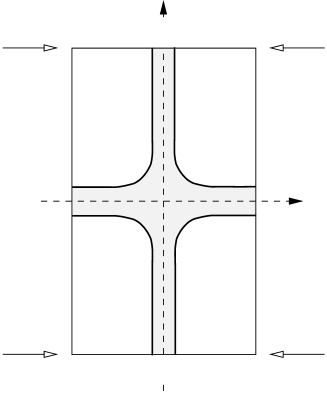
Figure 6: Boundary conditions on the world sheet. The initial $(l)$ and final $(r)$ solitons are located at the bottom and top sides of the rectangle at $t=-T/2$ and $t=T/2$, with the center of the energy density positioned at $x=0$. Periodic (modulo $2\pi$) boundary conditions apply to the left and right side of the rectangle. The shaded area significantly contributes to the action.

The contour of the integrals in Eq. (32) follows the edges of the rectangle in Fig. 6. Special care must be taken with the integrals over the vertical edges, at $x=\pm L/2$. Naively, one might think that these contributions vanish, but because both the superpotential and the field are multi-valued, these integrals do in fact contribute.

Before calculating the integrals in Eq. (32), let us first determine the dominant contribution from the vertical wall in the large $L$ limit. As stated in Section 2, this contribution is just $L$ times the tension $\sigma$ of the horizontal “wall” in Fig. 6. If $L$ is large, then the absolute value of $B$, the parameter that marks the $(r)$ and $(l)$ solitons, becomes large. In fact, the absolute value of $B$ increases logarithmically with $L$. Except for points in space near the center of the soliton where the energy density is maximal, the soliton field is approximately equal to $\pm\pi\pm\imath B$, where the second $\pm$ refers to the $(r)$ and $(l)$ soliton, respectively. For $\delta=\pm\pi/2$, there is a solution to the BPS equation that takes the form $\phi=\pm\pi+\imath f(t)$, where $f(t)\to\pm\infty$ for $t\to\pm\infty$. The tension of the horizontal “wall” $\sigma$ is equal to the tension of this solution. The leading contribution to $\Delta A$, linear in $L$, is therefore

$$\Delta A=\sigma L+\cdots=\frac{32\pi L}{\sqrt{3}}\,{\rm arctanh}\left(\frac{1}{\sqrt{3}}\right)+\cdots,$$ (33)

where the ellipsis indicate subleading terms in $L$. We will now uncover these subleading terms, which contribute to the pre-exponential factor in the tunneling amplitude. We will first determine the contributions from the spokes in Fig. 6 and then the hub.

Spoke contributions

We first simultaneously calculate the contributions of the first integral in Eq. (32) over the left and right edges of the rectangle in Fig. 6,

$$A_{1}=2\int_{-T/2}^{T/2}\!\!\!\!dt\,\left[\left.{\rm Re}\left({\mathcal{W}}\right)\right|_{x=L/2}-\left.{\rm Re}\left({\mathcal{W}}\right)\right|_{x=-L/2}\right].$$ (34)

In order to calculate $A_{1}$, it is necessary to exploit some symmetries of the soliton solutions. Apart from the translational invariance (modulo $2\pi$)

$$\phi(x+L)=2\pi+\phi(x),$$ (35)

the soliton solutions have the following two symmetry properties

$${\rm Re}\left[\phi(L/2+x)\right]=2\pi-{\rm Re}\left[\phi(L/2-x)\right],$$ (36)

and

$${\rm Im}\left[\phi(L/2+x)\right]={\rm Im}\left[\phi(L/2-x)\right].$$ (37)

If the symmetry in Eq. (36) is preserved by the instanton configuration, the interpolating field necessarily takes the form

$$\begin{array}[]{l}\phi(L/2,t)=\pi+\imath B(L,t)\\ \phi(-L/2,t)=-\pi+\imath B(L,t),\end{array}$$ (38)

at the left and right edges of the rectangle in Fig. 6, at $x=\pm L/2$, where $B(L,t)$ is a function interpolating between $-B(L)$ at $t=-T/2$ and $B(L)$ at $t=T/2$. However, from the identity

$${\mathcal{W}}(\pm\pi+\imath B)\equiv\frac{8\pi}{\sqrt{3}}\left[\pm\frac{\pi}{2}+\imath\,{\rm arctanh}\left(\frac{1}{\sqrt{3}}\tanh\frac{B}{2}\right)\right],$$ (39)

it is clear that the difference between the two integrands above does not depend on the function $B(L,t)$ at all. The contribution $A_{1}$ is therefore given by

$$A_{1}=\frac{16\pi^{2}}{\sqrt{3}}T.$$ (40)

This is just $T$ times the BPS bound on the soliton mass, or the Euclidean action in the absence of the tunneling transition.

Next, we simultaneously calculate the contributions of the first integral in Eq. (32) over the top and bottom edges of the rectangle in Fig. 6,

$$A_{2}=2\int_{-L/2}^{L/2}\!\!\!\!dx\,\left[\left.{\rm Im}\left({\mathcal{W}}\right)\right|_{t=T/2}-\left.{\rm Im}\left({\mathcal{W}}\right)\right|_{t=-T/2}\right].$$ (41)

Here the integrands are just the constants of motion for the soliton solutions, so that $A_{2}=2I_{r}-2I_{l}=4I_{r}$, and $I_{r}$ and $I_{l}$ mark the $(r)$ and the $(l)$ soliton, respectively. Therefore, in terms of $B(L)$, the value of $B$ that marks the $(r)$ soliton for a compact dimension with circumference $L$, we obtain

$$A_{2}=\frac{32\pi}{\sqrt{3}}\,L\,{\rm arctanh}\left(\frac{1}{\sqrt{3}}\tanh\frac{B(L)}{2}\right).$$ (42)

For large $L$, such that $B(L)\gg 2$, this reduces to $A_{2}=\sigma L$, the dominant contribution to the action that was already obtained in Eq. (33).

Hub contributions

We first simultaneously calculate the contribution of the second integral in Eq. (32) over the vertical edges in Fig. 6,

$$A_{3}=\int_{-T/2}^{T/2}\!\!\!\!dt\,\left[\left.{\rm Im}\left(\phi\partial_{t}\bar{\phi}\right)\right|_{x=L/2}-{\rm Im}\left.\left(\phi\partial_{t}\bar{\phi}\right)\right|_{x=-L/2}\right].$$ (43)

Using the form of $\phi$ for $x=\pm L/2$ given in Eq. (38), this contribution can be calculated and yields

$$A_{3}=-2\pi\int_{-T/2}^{T/2}dt\,\partial_{t}B(L,t)=-4\pi B(L).$$ (44)

Finally, we simultaneously calculate the contribution of the second integral in Eq. (32) over the horizontal edges in Fig. 6,

$$A_{4}=\int_{-L/2}^{L/2}\!\!\!\!dx\,\left[\left.{\rm Im}\left(\phi\partial_{x}\bar{\phi}\right)\right|_{t=-T/2}-\left.{\rm Im}\left(\phi\partial_{x}\bar{\phi}\right)\right|_{t=T/2}\right].$$ (45)

The $(r)$ and $(l)$ soliton are mapped onto each other by the transformation

$${\rm Im}[\phi(x)]\rightarrow-{\rm Im}[\phi(x)].$$ (46)

At the top and bottom edges of the rectangle in Fig. 6, the field $\phi$ therefore takes the form

$$\begin{array}[]{l}\phi(x,T/2)=a(x)+\imath b(x),\\ \phi(x,-T/2)=a(x)-\imath b(x),\end{array}$$

where $a(x)$ and $b(x)$ are real, and $a(\pm L/2)=\pm\pi$ and $b(\pm L/2)=B(L)$. The integral can now be calculated and yields

$$A_{4}=-2\int_{-L/2}^{L/2}dx\,\left(a\partial_{x}b-b\partial_{x}a\right)=4\pi B(L)-2S(L),$$ (47)

where

$$S(L)=2\int_{-L/2}^{L/2}dx\,b\partial_{x}a=2\int_{x=-L/2}^{x=L/2}da\,b=2\int_{-\pi}^{\pi}da\,b,$$ (48)

is the area in the complex $\phi$ plane between the $(l)$ and $(r)$ soliton configurations (see Fig. 7).

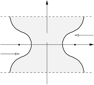
Figure 7: The $(r)$ and $(l)$ solitons and the instanton in the complex $\phi$ plane (compare Fig.(6) for the same configuration on the world sheet). The area $S(L)$ is indicated by the shaded region.

The hub contribution to the action is thus seen to be equal to minus twice the area traced by the instanton in the complex $\phi$ plane, $A_{\rm hub}=A_{3}+A_{4}=-2S(L)$. In Ref.[9] it was shown, within the context of domain wall junctions, that this result is valid in general and goes beyond the specific model we consider here. We also note that $A_{\rm hub}$ is negative, in agreement with the general considerations in Ref. [12]. The total semi-classical Euclidan tunneling action is

$$\Delta A_{\mathrm{BPS}} = A_{2}+A_{3}+A_{4},$$ (49)

$$= \frac{32\pi}{\sqrt{3}}\,L\,{\mathrm{arctanh}}\left(\frac{1}{\sqrt{3}}\tanh\frac{B(L)}{2}\right)-2S(L).$$

We have calculated each contribution in terms of the functions $B(L)$ and $S(L)$. These functions depend only on the initial and the final soliton configuration. In the large $L$ limit they take the form

$$S(L)=2\pi\log L+\cdots,$$ (50)

and

$$B(L)=\log L+\cdots,$$ (51)

where the ellipsis indicate terms that are finite or suppressed. We observe that the hub contribution depends logarithmically on $L$, in contrast with the situation for the domain wall junctions in models with infinite space dimensions, for example those considered in [11, 12], where the hub contribution to the energy of the junction is finite. The difference is that for those models the energy density falls off exponentially fast away from the domain walls, whereas in the present model the energy density only falls off like the second power of the inverse distance to the wall. The circumference $L$ of the compact dimension in a sense acts like an infrared regulator. In the large $L$ limit, the dominant and subdominant terms in tunneling action are given by

$$\Delta A\sim\frac{32\pi}{\sqrt{3}}\,L\,{\mathrm{arctanh}}\frac{1}{\sqrt{3}}-4\pi\log L+\cdots,$$ (52)

where the subdominant term contributes to the pre-exponential factor in the tunneling amplitude.

3.3.2 BPS saturation of the instanton configuration

The calculation in the previous section of the tunneling action hinges on the question whether a BPS saturated instanton configuration exists. The explicit form of such a configuration is not needed. In this section we use numerical analysis to address the question if a BPS saturated instanton configuration exists in this specific model. In order to numerically determine the instanton configuration, we embedded the model in $d=2+1$ dimensions. One of the space dimensions is compact and the other space dimension represents the original Euclidean time. The new time is just an auxiliary construction. An initial configuration smoothly interpolates between the $(l)$ and $(r)$ solitons. The second order equations of motions are then evaluated and at the same time the system is cooled. The instanton configuration then emerges as a domain wall junction.

We simulated the second order equations of motion on a lattice using a forward predicting algorithm similar to the one used in [11, 12]. A complication arises due to the fact that both space and the target space have the topology of a cylinder, so that proper periodic boundary conditions had to be implemented.

Figure 8: Comparison between the BPS bound on the tunneling action from Eq. (49) (solid line) and the actual semi-classical tunneling action from the numerical calculation (dots). It is clear that the actual instanton configuration saturates the BPS bound.

The lattice spacing was chosen to be much smaller than the width of the solitons. At the same time the size of the lattice was taken to be much larger than the soliton width. We performed the numerical calculation of the tunneling action for values of $L$ ranging from $L=2$ up to $L=6$. The semi-classical tunneling action is only physically meaningful for larger values of $L$. However, the computation time increases rapidly with $L$. As shown in Fig. 8, the calculated value for the tunneling action with the numerically determined instanton configuration saturates the BPS bound in Eq. (49). As there is no reason to think otherwise, we are confident that this saturation also occurs for larger values of $L$.

4 Quantum-mechanical description

Under certain conditions on the superpotential ${\cal W}$ (and the Kähler potential $\cal{K}$, if it is non-trivial) it may be possible to develop a quantum-mechanical description of the tunneling of the distinct solitons resulting in the loss of their BPS saturation. Such an approach is valid provided there is a certain direction in the functional space which is much softer than all other “perpendicular” directions, and the tunneling occurs in this “soft” direction. Then all “perpendicular” degrees of freedom (there are infinitely many of them) can be integrated out and what is left is the quantum-mechanical motion of the center of mass plus the quantum mechanical dynamics of this particular soft degree of freedom. The motion of the center of mass is irrelevant, of course. It is always assumed that the soliton is at rest.

The example considered in Section 3 contains no adjustable parameters (except $L$), so that one does not expect to find a specifically soft excitation mode in the soliton background. Therefore, in this case the quantum-mechanical description (with one bosonic variable) would describe the system only qualitatively. It is not difficult, however, to modify the superpotential to create a soft mode. To this end, let us consider the superpotential

$$d{\mathcal{W}}=\frac{4\pi}{2-\beta\cos\Phi}d\Phi\,,$$ (53)

which introduces a parameter $\beta$ in the superpotential (17), without changing anything else. At very small $\beta$ and large $L$,

$$\log\frac{4}{\beta}\gg L\gg 1,$$ (54)

the $x$ dependence of the imaginary part of $\phi$ becomes weak, and the softest mode corresponding to varying ${\rm Im}(\phi)$ is much softer than all other modes. (We treat $L$ as a fixed parameter, while $\beta$ can be made as small as desired.) Then we can define our quantum mechanical variable $B$ such that $B$ is the value of ${\rm Im}(\phi)$ (for definiteness, at ${\rm Re}(\phi)=\pm\pi$). At the classical equilibrium

$$B_{0}=\pm\log(L/\beta)+{\rm const.}\,\qquad(L\gg 1)\,.$$ (55)

The positive value of $B_{0}$ corresponds to the $(r)$ soliton, the negative to the $(l)$ soliton. Both are classically BPS saturated. To roll over from positive to negative $B$, the system has to tunnel under the barrier at $B=0$.

Before passing to the discussion of supersymmetric quantum mechanics for the variable $B$ we have to present a few formula from Section 3 in a modified form which includes the parameter $\beta$, see Eq. (53).

The superpotential with the additional parameter $\beta$ takes the form

$${\cal W}=\frac{8\pi}{\sqrt{4-\beta^{2}}}\arctan\left(\sqrt{\frac{2+\beta}{2-\beta}}\tan\frac{\phi}{2}\right).$$ (56)

The poles of the scalar potential are located on the imaginary axis at

$$\phi=\pm\imath\log\frac{2}{\beta}\left(1+\sqrt{1-\frac{\beta^{2}}{4}}\right),$$ (57)

so at small $\beta$ they move further away from each other. The energy of the classical BPS saturated soliton is

$$M_{\rm BPS}\equiv Z=\frac{16\pi^{2}}{\sqrt{4-\beta^{2}}}\to 8\pi^{2}\,\,\,\mbox{at}\,\,\,\beta\to 0.$$ (58)

Finally, in the limit of large $L$ the sphaleron energy is equal to

$$M_{\rm sphal} = M_{\rm BPS}-\frac{32\pi}{\sqrt{4-\beta^{2}}}\arctan\frac{\sqrt{2-\beta}}{\sqrt{\beta}}+\frac{16\pi}{2+\beta}\log\frac{\sqrt{2+\beta}+\sqrt{\beta}}{\sqrt{2+\beta}-\sqrt{\beta}}$$ (59)

$$+\frac{16\pi^{2}}{(2+\beta)^{2}}L$$

$$\to M_{\rm BPS}+4\pi^{2}L+{\rm const.}\,\,\,\mbox{at}\,\,\,\beta\to 0.$$

We recall that the difference between the sphaleron energy and the classical soliton mass measures the height of the tunneling barrier. The tunneling action as a function of $\beta$ becomes

$$\Delta A=\frac{32\pi L}{\sqrt{4-\beta^{2}}}{\rm arctanh}\sqrt{\frac{2-\beta}{2+\beta}}\to 8\pi L\log\frac{4}{\beta}\,\,\,\mbox{at}\,\,\,\beta\to 0.$$ (60)

Now we pass to the quantum-mechanical treatment. To begin, let us recall some general aspects. A general algebraic consideration of the BPS soliton dynamics in the extreme non-relativistic limit is carried out in [16]. We will adapt it here for our purposes.

The superalgebra we deal with has four supercharges and a central charge $Z$ (the latter is real in the problem at hand). In the extreme nonrelativistic limit it can be represented as [16] (in the soliton rest-frame)

$$Q_{2}^{1} = \sqrt{2Z}\tau_{1}\otimes\sigma_{3}+...\,,\qquad\quad Q^{2}_{1}=\sqrt{2Z}\tau_{2}\otimes\sigma_{3}+...\,,$$

$$Q_{1}^{1} = I\otimes\frac{1}{2\sqrt{m}}\left[p\sigma_{1}+W^{\prime}(B)\sigma_{2}\right]\,,\quad Q_{2}^{2}=I\otimes\frac{1}{2\sqrt{m}}\left[p\sigma_{2}-W^{\prime}(B)\sigma_{1}\right]\,,$$ (61)

where

$$p=-id/dB$$

and $m$ is an effective inertia coefficient for the variable $B$ (“mass”). The dots in the first line in Eq. (61) stand for higher order terms in the nonrelativistic expansion. Moreover, $W(B)$ is the quantum-mechanical superpotential (not to be confused with the field-theoretic superpotential ${\cal W}$). The algebra (61) has, as its subalgebra, Witten’s quantum mechanics [17].

In principle, $W(B)$ could be calculated from the underlying field theory, in the same way as it was done in a related problem in Ref. [16]. We will not do this calculation in full, since our purpose here is mainly illustrative. Instead, we will present a simplified superpotential which properly conveys qualitative features of the actual superpotential: (i) the existence of two zeros of $W^{\prime}(B)$ at $B=\pm|B_{0}|$ (double-well potential); (ii) the existence of the barrier at $B$ near zero, with the maximum at zero, and with the height coinciding with $M_{\rm sphal}-Z=4\pi^{2}L$.

The corresponding superpotential and Hamiltonian have the form

$$W = k\left(-\frac{B^{3}}{3}+B_{0}^{2}B\right),$$

$$H = \frac{p^{2}}{2m}+\frac{1}{2m}(W^{\prime})^{2}+\frac{1}{{2m}}\sigma_{3}W^{\prime\prime}\,,$$ (62)

where

$$B_{0} = \log L/\beta$$

$$k = 6\pi L\frac{\log 4/\beta}{\log^{3}L/\beta}$$ (63)

$$m = \frac{9}{2}L\frac{\log^{2}4/\beta}{\log^{2}L/\beta}$$

(Note that the overall two-by-two unit matrix following from the second line in Eq. (61) is omitted in $H$. Its just replicates the states, in two copies each. We will keep it in mind.)

$B_{0}^{2}$ is a function of $L$, which is logarithmically large and positive at large $L$. As $L$ decreases, $B_{0}^{2}$ decreases too, and goes to zero at $L=1$. (To see that this is the case, one should inspect the exact expression for $B_{0}$ rather than the asymptotic form in Eq.(4) valid at large $L$.) Below this point $B_{0}^{2}<0$, and the Hamiltonian has no supersymmetric solution at the classical level. The Witten index of the system under consideration is zero.

At positive $B_{0}^{2}$ there are two classical solutions of the equation $W^{\prime}=0$, corresponding to two classical vacua. The tunneling between them was thoroughly studied, see e.g. [18]. The one-instanton action is obviously

$$A_{\rm inst}=\left[W(B=|B_{0}|)-W(B=-|B_{0}|)\right]\equiv\Delta W=\frac{4k}{3}|B_{0}|^{3}.$$ (64)

The instanton transition is accompanied by a fermion zero mode, which suppresses all one-instanton amplitudes. The shift of the ground state from zero is given by the instanton–anti-instanton transition and is proportional to $\exp(-2A_{\rm inst})$ (for further details see [18]). This can also clearly be seen from the Hamiltonian (62) which has a strictly conserved quantum number, $[\sigma_{3},H]=0$. The one-instanton transition would flip the spin. The ground state of the Hamiltonian (62) is doubly degenerate, with one spin-up and one spin-down state of energy $E\sim\exp(-2A_{\rm inst})$. If we include, in addition, the replication (which was mentioned above) due to the two-by-two unit matrix, we get that the overall number of states is four, as it must be in any non-BPS ${\cal N}=2$ supermultiplet.

To conclude this section, we stress again that although the superpotential specified in Eqs.(62) and (4) correctly reproduces gross features of the tunneling phenomenon, it is definitely not the genuine superpotential that might arise in this problem should we decide to actually calculate it. In particular, it vanishes at small $\beta$ only logarithmically, while actually one could expect a power-type suppression.

5 Conclusions

In a previous work, Ref.[5], it was observed that in certain $(1+1)$-dimensional models with ${\cal N}=2$ supersymmetry and a compact space dimension, tunneling between two distinct, classically BPS saturated solitons lifts their mass above the BPS bound. The two shortened multiplets combine to form one regular ${\cal N}=2$ multiplet. One of the main new assertions in this paper is that the instanton that interpolates between the solitons in the Euclidean time is a $1/4$ BPS saturated “domain wall junction.” The semi-classical instanton action is determined by two central charges in the supersymmetry algebra. The action can therefore be determined solely from the solitons that are connected by the instanton; an explicit instanton solution is not necessary.

Under certain conditions the description of the tunneling between the solitons in the field theory can be reduced to a non-relativistic supersymmetric quantum mechanical model. This approach is valid if the direction in the functional space in which the tunneling takes place is much softer than all other directions (except for the zero modes), yet the tunneling action is large. The internal coordinate along this direction then forms the one remaining degree of freedom after all hard degrees of freedom have been “integrated out.”

We illustrated the above observations explicitly in a specific model. The semi-classical tunneling action was determined in the field theory. We used numerical methods to verify that the instanton indeed corresponds to the $1/4$ BPS saturated domain wall junction. We also determined a range of parameters for which the tunneling can be described by a quantum mechanical model. Although possible in principle, we did not determine the actual superpotential of the quantum mechanical model in this range. Instead, we determined the parameters of a toy superpotential that is similar to the actual superpotential in all important features.

References

- [1] G. Dvali and M. Shifman, Nucl. Phys. B 504, 127 (1997), hep-th/9611213.
- [2] N. Arkani-Hamed, S. Dimopoulos, G. Dvali, Phys. Lett. B 429, 263 (1998), hep-ph/9803315; N. Arkani-Hamed, S. Dimopoulos, G. Dvali, Phys. Rev. D 59, 086004 (1999), hep-ph/9807344.
- [3] Y. Meurice and B. Veneziano, Phys. Lett. B141, 69 (1984).
- [4] I. Affleck, M. Dine and N. Seiberg, Nucl. Phys. B241, 493 (1984); Phys. Rev. Lett. 52, 1677 (1984).
- [5] X. Hou, A. Losev and M. Shifman, Phys. Rev. D 61, 085005 (2000), hep-th/9910071.
- [6] J. A. de Azcárraga, J. P. Gauntlett, J. M. Izquierdo and P. K. Townsend, Phys. Rev. Lett. 63, 2443 (1989).
- [7] E. R. C. Abraham and P. K. Townsend, Nucl. Phys. 351, 313 (1991); M. Cvetic, F. Quevedo and S. J. Rey, Phys. Rev. Lett. 67, 1836 (1991).
- [8] G. W. Gibbons and P. K. Townsend, Phys. Rev. Lett. 83, 1727 (1999), hep-th/9905196.
- [9] S. M. Carroll, S. Hellerman and M. Trodden, Phys. Rev. D 61, 065001 (2000), hep-th/9905217.
- [10] A. Gorsky and M. Shifman, Phys. Rev. D 61, 085001 (2000), hep-th/9909015.
- [11] D. Binosi and T. ter Veldhuis, Phys. Lett. B 476, 124 (2000), hep-th/9912081.
- [12] M. Shifman and T. ter Veldhuis, Calculating the tension of domain wall junctions and vortices in generalized Wess-Zumino models, hep-th/9912162.
- [13] S. Cecotti, P. Fendley, K. Intriligator, C. Vafa, Nucl. Phys. B 386, 405 (1992), hep-th/9204102.
- [14] B. Chibisov and M. Shifman, Phys. Rev. D56, 7990 (1997), hep-th/9706141; Erratum-ibid. D58 109901 (1998).
- [15] R. Dashen, B. Hasslacher and A. Neveu, Phys. Rev. D10, 4138 (1974); F. R. Klinkhamer and N. S. Manton, Phys. Rev. D30, 2212 (1984). For a review see V. Novikov et al., ABC of Instantons, in M. Shifman, ITEP Lectures on Particle Physics and Field Theory (World Scientific, Singapore 1999), Vol. 1, p. 258.
- [16] A. Ritz, M. Shifman, A. Vainshtein and M. Voloshin, to be published.
- [17] E. Witten, Nucl. Phys. B 188, 513 (1981).
-
[18]
P. Salomonson and J. W. van Holten,
Nucl. Phys. B196, 509 (1982);
M. Claudson and M. B. Halpern, Nucl. Phys. B250, 689 (1985).