Extended BRS Symmetry and Gauge Independence in On-Shell Renormalization Schemes

Abstract

Extended BRS symmetry is used to prove gauge independence of the fermion renormalization constant $Z_{2}$ in on-shell QED renormalization schemes. A necessary condition for gauge independence of $Z_{2}$ in on-shell QCD renormalization schemes is formulated. Satisfying this necessary condition appears to be problematic at the three-loop level in QCD.

In on-shell schemes, the fermion mass renormalization $Z_{m}$ and wave function renormalization $Z_{2}$ have been observed to be gauge parameter independent in explicit two-loop QED and QCD calculations [1]. Gauge parameter independence of $Z_{2}$ is phenomenologically significant because it implies that the difference between the (fermion) anomalous dimension of heavy quark effective theories [2] and QCD is gauge independent.

An extension of BRS symmetry, which allows variations of the gauge parameter to be included as part of the symmetry transformations [3], will be applied to the gauge parameter dependence of $Z_{2}$. This approach results in an extension of Slavnov-Taylor identities, allowing gauge dependence to be formulated algebraically. Previous application of these techniques resulted in a proof of the gauge independence of the mass renormalization $Z_{m}$ to all orders in on-shell QED and QCD renormalization schemes [4]. We will prove the gauge parameter independence of $Z_{2}$ in on-shell schemes for QED and formulate a necessary condition for gauge independence in QCD which appears problematic beyond the two-loop level. This complements earlier work on gauge independence of $Z_{2}$ in QED resulting in the (dimensionally-regularized) relation [5]

$$\frac{\partial Z_{2}}{\partial\xi}\sim\int d^{D}k\frac{1}{k^{4}}=0$$ (1)

where $\xi$ is the gauge parameter and the massless tadpole is zero in dimensional regularization. Since the QED result (1) cannot be extended to QCD, our extended BRS symmetry proof for QED provides a new approach to formulating questions of gauge independence of $Z_{2}$ in QCD.

The QED Lagrangian in the auxiliary field formalism [6] for covariant gauges is

$${\cal L}=-\frac{1}{4}F^{2}+\bar{\psi}\left(i{D}\!\!\!/-m\right)\psi+\frac{\xi}{2}B^{2}+B\partial\cdot A-\bar{c}\partial^{2}c$$ (2)

where $F$ is the field strength and $B$ is the auxiliary gauge field. This Lagrangian is invariant under the BRS symmetry

$$\delta A_{\mu}=\epsilon\partial_{\mu}c\quad,\quad\delta\bar{\psi}=i\epsilon gc\bar{\psi}\quad,\quad\delta c=0$$

$$\delta B=0\quad,\quad\delta\psi=-i\epsilon gc\psi\quad,\quad\delta\bar{c}=0$$ (3)

where $\epsilon$ is a global grassmann quantity. The auxiliary field formalism guarantees nilpotence of the BRS transformations without invoking equations of motion.

An extension of BRS symmetry that includes gauge parameter variations introduces a new term in the Lagrangian

$${\cal L}\rightarrow{\cal L}+\frac{\chi}{2}\bar{c}B$$ (4)

where $\chi$ is a global grassmann variable. Although $\chi$ will be set to zero after functional differentiation, it is still important to recognize that since $\chi$ is a global Grassmann quantity, it does not change the dynamics of any process with zero ghost number. The modified Lagrangian (4) is invariant under the following extended BRS symmetry [3]

$$\delta^{+}A_{\mu}=\epsilon\partial_{\mu}c\quad,\quad\delta^{+}\bar{\psi}=i\epsilon gc\bar{\psi}\quad,\quad\delta^{+}c=0$$

$$\delta^{+}B=0\quad,\quad\delta^{+}\psi=-i\epsilon gc\psi\quad,\quad\delta^{+}\bar{c}=B$$ (5)

$$\delta^{+}\xi=\epsilon\chi\quad,\quad\delta^{+}\chi=0$$ (6)

As for BRS symmetry, the extended BRS symmetry (5) implies the the following relation for the effective action $\Gamma$.

$$0=\partial_{\mu}c\frac{\delta\Gamma}{\delta A_{\mu}}+\frac{\delta\Gamma}{\delta\bar{K}}\frac{\delta\Gamma}{\delta\psi}+\frac{\delta\Gamma}{\delta K}\frac{\delta\Gamma}{\delta\bar{\psi}}+B\frac{\delta\Gamma}{\delta\bar{c}}+\chi\frac{\partial\Gamma}{\partial\xi}$$ (7)

where $K$ is a current coupled to the composite operator $\delta^{+}\bar{\psi}$ and $\bar{K}$ is coupled to $\delta^{+}\psi$. Differentiating (7) with respect to $\chi$, $\bar{\psi}(x)$, $\psi(y)$, setting $\chi=0$ and imposing ghost number conservation leads to the following identity for the proper fermion two-point function [4].

$$\frac{\partial}{\partial\xi}\frac{\delta^{2}\Gamma}{\delta\psi(y)\delta\bar{\psi}(x)}=+\frac{\delta^{3}\Gamma}{\delta\psi(y)\delta\bar{K}\delta\chi}\frac{\delta^{2}\Gamma}{\delta\bar{\psi}(x)\delta\psi}+\frac{\delta^{2}\Gamma}{\delta\psi(y)\delta\bar{\psi}}\frac{\delta^{3}\Gamma}{\delta\bar{\psi}(x)\delta K\delta\chi}$$ (8)

Transforming to momentum space and defining

$$\frac{\delta^{2}\Gamma}{\delta\chi\delta{\bar{K}}(w)\delta\psi(y)}=\int\frac{d^{4}q}{(2\pi)^{4}}\frac{d^{4}\ell}{(2\pi)^{4}}\,e^{-iq\cdot(y-z)-i\ell\cdot(w-z)}F(q,\ell,-q-\ell)$$ (9)

$$\frac{\delta^{2}\Gamma}{\delta\chi\delta K(w)\delta{\bar{\psi}}(y)}=\int\frac{d^{4}q}{(2\pi)^{4}}\frac{d^{4}\ell}{(2\pi)^{4}}\,e^{-iq\cdot(x-z)-i\ell\cdot(w-z)}{\bar{F}}(q,\ell,-q-\ell)$$ (10)

results in the final form needed for studying the gauge dependence of the fermion propagator $S_{F}$ in QED [4].

$$\frac{\partial}{\partial\xi}S_{F}^{-1}(p)=S_{F}^{-1}(p)\left[F(p,-p,0)+\bar{F}(-p,p,0)\right]$$ (11)

Note that the Green functions $F(p,-p,0)$ and $\bar{F}(p,-p,0)$ cannot have single particle poles.

In on-shell renormalization schemes the bare mass $m_{0}$ and the renormalized mass $M$ are related through the condition

$$\biggl{.}S_{F}^{-1}(p)\biggr{|}_{{p}\!\!\!/=M}=0$$ (12)

This results in the definition of the mass renormalization constant.

$$\frac{m_{0}}{M}=Z_{m}$$ (13)

The wave function renormalization constant $Z_{2}$ is the residue of $S_{F}$ at the ${p}\!\!\!/=M$ pole.

$$Z_{2}=\lim_{{p}\!\!\!/=M}\left({p}\!\!\!/-M\right)S_{F}(p)$$ (14)

Perturbative expansions of $Z_{m}$ and $Z_{2}$ have been calculated to two-loop order in a scheme which dimensionally regulates both the infrared and ultraviolet divergences, resulting in explicitly gauge independent expressions for QED and QCD [1].

The mass renormalization $Z_{m}$, and hence $M$, has been proven to be gauge independent to all orders of perturbation theory [4, 7]. Thus when both sides of (11) are divided by ${p}\!\!\!/-M$ the quantity ${p}\!\!\!/-M$ commutes with the $\xi$ derivative.

$$\frac{\partial}{\partial\xi}\left(\frac{S_{F}^{-1}(p)}{{p}\!\!\!/-M}\right)=\frac{S_{F}^{-1}(p)}{{p}\!\!\!/-M}\left[F(p,-p,0)+\bar{F}(-p,p,0)\right]$$ (15)

Using the property that

$$S_{F}^{-1}(p)=\frac{{p}\!\!\!/-M}{Z_{2}}+{\cal O}\left[\,\left({p}\!\!\!/-M\right)^{2}\,\right]$$ (16)

along with the gauge independence of $M$ leads to the following result when (15) is evaluated on-shell.

$$\frac{\partial}{\partial\xi}\left(\frac{1}{Z_{2}}\right)=\frac{1}{Z_{2}}\lim_{{p}\!\!\!/=M}\left[F(p,-p,0)+\bar{F}(-p,p,0)\right]$$ (17)

This is our central result for QED: the gauge dependence of the wave function renormalization constant is related to the on-shell properties of the Green function $F(p,-p,0)+\bar{F}(p,-p,0)$. In particular, if this Green function is zero on-shell, then $Z_{2}$ is gauge independent.

Before studying the on-shell behaviour of $F(p,-p,0)+\bar{F}(p,-p,0)$ we review some aspects of the auxiliary field formalism. Since the $B$ field and $\partial\cdot A$ are mixed in the Lagrangian (2) the quadratic part of the Lagrangian must be diagonalized, leading to the free field propagators

$$\int d^{4}x\,e^{ip\cdot x}\langle O|T\left(B(x)B(0)\right)|O\rangle=0$$ (18)

$$\int d^{4}x\,e^{ip\cdot x}\langle O|T\left(B(x)A_{\mu}(0)\right)|O\rangle=\frac{p_{\mu}}{p^{2}}\equiv G_{\mu}(p)$$ (19)

$$\int d^{4}x\,e^{ip\cdot x}\langle O|T\left(A_{\mu}(x)A_{\nu}(0)\right)|O\rangle=i\left[-\frac{g^{\mu\nu}}{p^{2}}+(1-\xi)\frac{p^{\mu}p^{\nu}}{p^{4}}\right]\equiv D^{\mu\nu}(p)$$ (20)

BRS symmetry implies that (18) and (19) are valid to all orders in perturbation theory [4].

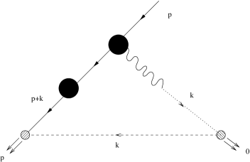
As illustrated in Figure 1, the (QED) Green function $F(p,-p,0)$ is easily written in terms of one-particle irreducible Green functions

$$F(p,-p,0)=\int d^{D}k\,\Gamma_{\mu}(k,p)G_{\mu}(k)S_{F}(p+k)\tilde{D}(k^{2})$$ (21)

where $\tilde{D}(k^{2})$ is the ghost propagator (which for QED corresponds to the free field result) and the fermion-photon vertex function $\Gamma_{\mu}$ is defined by

$$S_{F}(p)\Gamma_{\nu}(p,k)S_{F}(p+k)D^{\mu\nu}(k)=\int d^{D}x\int d^{D}y\,\,e^{ik\cdot x+ip\cdot y}\langle O|T\left[\psi(0)A_{\mu}(x)\bar{\psi}(y)\right]|O\rangle$$ (22)

Substituting (19) and the (free-field) ghost propagator into (21) and using the Ward identity for the vertex function

$$k^{\mu}\Gamma_{\mu}(p,k)=S_{F}^{-1}(p+k)-S_{F}^{-1}(p)$$ (23)

simplifies the expression for $F(p,-p,0)$.

$$F(p,-p,0)=iS_{F}^{-1}(p)\int d^{D}k\frac{1}{k^{4}}S_{F}(p+k)-i\int d^{D}k\frac{1}{k^{4}}$$ (24)

The second term in the above equation is a massless tadpole which is zero in dimensional regularization, leading to the final expression for $F(p,-p,0)$ in QED.

$$F(p,-p,0)=iS_{F}^{-1}(p)\int d^{D}k\frac{1}{k^{4}}S_{F}(p+k)$$ (25)

In the on-shell scheme [1] infrared and ultraviolet divergences are dimensionally regulated, so the integral in (25) is finite on-shell. Thus the $S_{F}^{-1}(p)$ prefactor in (25) implies that $F(p,-p,0)$ is zero at the ${p}\!\!\!/=M$ mass-shell. This argument can be trivially extended to $\bar{F}(p,-p,0)$, and we conclude that to all orders in QED

$$\biggl{.}F(p,-p,0)+\bar{F}(p,-p,0)\biggr{|}_{{p}\!\!\!/=M}=0$$ (26)

and hence from the result (17) we have proven the gauge independence of the QED renormalization constant $Z_{2}$ in mass-shell schemes.

Figure 1: Feynman diagram expressing $F(p,-p,0)$ in terms of one-particle irreducible functions represented by the solid circles. Dashed lines represent the ghost field, and the dotted line represents the auxiliary field $B$. Composite operators coupled to the currents are represented by the partially-filled circles.

An explicit illustration of the on-shell behaviour of $F(p,-p,0)+\bar{F}(p,-p,0)$ in the regularization scheme [1] to one-loop order requires evaluation of the diagram in Figure 2. In terms of the integrals (with the convention $D=4+2\epsilon$)

$$\int\frac{d^{D}k}{(2\pi)^{D}}\frac{1}{\left[(k-p)^{2}-m_{0}^{2}\right]^{\alpha}\,k^{2\beta}}=I\left[\alpha,\beta\right]$$ (27)

$$\int\frac{d^{D}k}{(2\pi)^{D}}\frac{k^{\mu}}{\left[(k-p)^{2}-m_{0}^{2}\right]^{\alpha}\,k^{2\beta}}=p^{\mu}J\left[\alpha,\beta\right]$$ (28)

we find the one-loop expression for $F(p,-p,0)+\bar{F}(p,-p,0)$.

$$F(p,-p,0)+\bar{F}(p,-p,0)=2ig^{2}\left[m_{0}\left({p}\!\!\!/-m_{0}\right)J(1,2)+\left(p^{2}+m_{0}^{2}\right)J(1,2)-I(1,1)\right]$$ (29)

and hence the on-shell behavior of $F+\bar{F}$ to one-loop order is given by

$$\lim_{{p}\!\!\!/=M}\left[F(p,-p,0)+\bar{F}(p,-p,0)\right]=2ig^{2}\lim_{{p}\!\!\!/=M=m_{0}}\left[2m_{0}^{2}J(1,2)-I(1,1)\right]$$ (30)

The desired on-shell values for the integals in (30) can be reduced to evaluation of a single class of scalar integrals.

$$\Lambda\left[\alpha,\beta\right]=\int\frac{d^{D}k}{(2\pi)^{D}}\frac{1}{\left[k^{2}+2p\cdot k\right]^{\alpha}\,k^{2\beta}}$$ (31)

a particular example being a relation between $J(\alpha,\beta)$ and $\Lambda(\alpha,\beta)$

$$\lim_{{p}\!\!\!/=m_{0}}J(\alpha,\beta)=\frac{1}{2m_{0}^{2}}\left[\Lambda(\alpha,\beta-1)-\Lambda(\alpha-1,\beta)\right]$$ (32)

The integration by parts technique [8] for these on-shell integrals leads to recursion relations among the $\Lambda(\alpha,\beta)$. The identities

$$0=\int d^{D}k\frac{\partial}{\partial k^{\mu}}\left(\frac{p^{\mu}}{\left[k^{2}+2p\cdot k\right]^{\alpha}\,k^{2\beta}}\right)$$ (33)

$$0=\int d^{D}k\frac{\partial}{\partial k^{\mu}}\left(\frac{k^{\mu}}{\left[k^{2}+2p\cdot k\right]^{\alpha}\,k^{2\beta}}\right)$$ (34)

lead to the recursion relations

$$0=-\beta\Lambda(\alpha-1,\beta+1)+(\beta-\alpha)\Lambda(\alpha,\beta)-2\alpha m_{0}^{2}\Lambda(\alpha+1,\beta)+\alpha\Lambda(\alpha+1,\beta-1)$$ (35)

$$0=(D-2\beta-\alpha)\Lambda(\alpha,\beta)-\alpha\Lambda(\alpha+1,\beta-1)$$ (36)

The recursion relation (36) can also be obtained from dimensional analysis. These recursion relations allow the on-shell behaviour of the one-loop integrals, after setting mass tadpoles to zero, to be reduced to the fundamental dimensional regularization result

$$\Lambda(\alpha,0)=\int\frac{d^{D}k}{(2\pi)^{D}}\frac{1}{\left[k^{2}-m_{0}^{2}\right]^{\alpha}}=\frac{i}{(4\pi)^{D/2}}\left(-m_{0}^{2}\right)^{2-\alpha}m_{0}^{2\epsilon}\frac{\Gamma(\alpha-2-\epsilon)}{\Gamma(\alpha)}$$ (37)

Using the above techniques it is simple to find the on-shell integrals required in (30).

$$J(1,2)=\frac{i}{(4\pi)^{D/2}}m_{0}^{2\epsilon}\frac{\Gamma(-\epsilon)}{2m_{0}^{2}(D-3)}$$ (38)

$$I(1,1)=\frac{i}{(4\pi)^{D/2}}m_{0}^{2\epsilon}\frac{\Gamma(-\epsilon)}{(D-3)}$$ (39)

and hence in the on-shell regularization scheme [1], the Green function $F+\bar{F}$ is zero on-shell to one-loop order, providing a specific example of our general result.

Figure 2: Feynman diagram for one-loop contributions to $F(p,-p,0)$. Dashed lines represent the ghost field, and the dotted line represents the auxiliary field $B$. Composite operators coupled to the currents are represented by the partially-filled circles.

The gauge dependence of $Z_{2}$ in QCD can be formulated in a similar fashion. Analogous to (4) the Lagrangian for QCD becomes

$${\cal L}=-\frac{1}{4}F^{2}+\bar{\psi}\left(i{D}\!\!\!/-m\right)\psi+\frac{\xi}{2}B^{2}+B\partial\cdot A-\bar{c}\partial^{\mu}D_{\mu}c+\frac{\chi}{2}\bar{c}B$$ (40)

which is invariant under an extended BRS symmetry

$$\delta^{+}A_{\mu}=\epsilon D_{\mu}c\quad,\quad\delta^{+}\bar{\psi}=i\epsilon gc\bar{\psi}\quad,\quad\delta^{+}c=-\frac{1}{2}\epsilon g\left[c,c\right]$$

$$\delta^{+}B=0\quad,\quad\delta^{+}\psi=-i\epsilon gc\psi\quad,\quad\delta^{+}\bar{c}=B$$ (41)

$$\delta^{+}\xi=\epsilon\chi\quad,\quad\delta^{+}\chi=0$$ (42)

The extended BRS symmetry (41) implies the following identity for the effective action nearly identical in form to the QED identity (7)

$$0=\frac{\delta\Gamma}{\delta K_{\mu}}\frac{\delta\Gamma}{\delta A_{\mu}}+\frac{\delta\Gamma}{\delta\bar{K}}\frac{\delta\Gamma}{\delta\psi}+\frac{\delta\Gamma}{\delta K}\frac{\delta\Gamma}{\delta\bar{\psi}}+B\frac{\delta\Gamma}{\delta\bar{c}}+\frac{\delta\Gamma}{\delta\bar{K}_{c}}+\chi\frac{\partial\Gamma}{\partial\xi}\frac{\delta\Gamma}{\delta c}$$ (43)

where $K_{\mu}$ and $\bar{K}_{c}$ are currents coupled to composite operators respectively coupled to the extended BRS variations of $A^{\mu}$ and $c$. Following the procedure used to develop (8) leads to a QCD expression in a similar form.

$$\frac{\partial}{\partial\xi}\frac{\delta^{2}\Gamma}{\delta\psi(y)\delta\bar{\psi}(x)}=+\frac{\delta^{3}\Gamma}{\delta\psi(y)\delta\bar{K}\delta\chi}\frac{\delta^{2}\Gamma}{\delta\bar{\psi}(x)\delta\psi}+\frac{\delta^{2}\Gamma}{\delta\psi(y)\delta\bar{\psi}}\frac{\delta^{3}\Gamma}{\delta\bar{\psi}(x)\delta K\delta\chi}$$ (44)

After transforming to momentum space we find a result identical in form to (11).

$$\frac{\partial}{\partial\xi}S_{F}^{-1}(p)=S_{F}^{-1}(p)\left[F(p,-p,0)+\bar{F}(-p,p,0)\right]$$ (45)

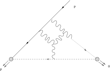
As in the QED case, we see that the necessary condition for gauge independence of $Z_{2}$ in QCD is for the Green function $F+\bar{F}$ to be zero on shell. The distinction between QED and QCD occurs in the interactions, particularly the ghost-gluon interaction, which will contribute to $F(p,-p,0)$. This is particularly evident at three loop level where diagrams (such as those in Figure 3) occur that cannot be related to the fundamental two- or three-point Green functions. Thus at three-loop level there is no simple extension of the result (21) from QED to QCD, and hence gauge independence of $Z_{2}$ in on-shell schemes seems problematic at the three-loop level and beyond in QCD.

Figure 3: A three-loop QCD diagram contributing to $F(p,-p,0)$ which cannot be reduced to the the form (21) composed of fundamental one-particle irreducible Green functions.

Acknowledgements: TGS is grateful for the financial support of the Natural Sciences and Engineering Research Council of Canada (NSERC). TGS thanks Martin Lavelle and Emilio Bagan for discussions at early stages of this work.

References

• [1] D.J. Broadhurst, N. Gray, K. Schilcher: Z. Phys. C52 (1991) 111.
• [2] N. Isgur, M. Wise: Phys. Lett. B232 (1989) 113.
• [3] O. Piguet, K. Sibold: Nucl. Phys. B253 (1985) 517.
• [4] J.C. Breckenridge, M.J. Lavelle, T.G. Steele: Z. Phys. C65 (1995) 155.
• [5] K. Johnson, B. Zumino: Phys. Rev. Lett. 3 (1959) 351; T. Fukuda, R. Kubo, K. Yokoyama: Prog. Theor. Phys. 63 (1980) 1384.
• [6] N. Nakanishi: Prog. Theor. Phys. 35 (1966) 1111; B. Lautrup: Mat. Fys. Medd. Dan. Vid. Selsk. 35 (1967) 29.
• [7] A.S. Kronfeld, Phys. Rev. D58 (1998) 051501
• [8] K.G. Chetyrkin, F.V. Tkachov: Nucl. Phys. B192 (1981) 159.