DESY 00-080

DIAS-STP-00-11

UNITU–THEP–6/2000

FSUJ-TPI-06/2000

hep-th/0005221

ADHM Construction of Instantons

on the Torus

C. Ford ^a, J. M. Pawlowski ^b, T. Tok ^c and A. Wipf ^d

^aDeutsches Elektronen-Synchrotron DESY-Zeuthen
Platanenalle 6, D-15738 Zeuthen, Germany
 ford@ifh.de

^bDublin Institute for Advanced Studies
10 Burlington Road, Dublin 4, Ireland
 jmp@stp.dias.ie

^cInstitut für Theoretische Physik, Universität Tübingen
Auf der Morgenstelle 14, D-72072 Tübingen, Germany
 tok@alpha6.tphys.physik.uni-tuebingen.de

^dTheoretisch Physikalisches Institut, Universität Jena
Fröbelstieg 1, D–07743 Jena, Germany
 wipf@tpi.uni-jena.de

We apply the ADHM instanton construction to $SU(2)$ gauge theory on ${\mbox{\af T}}^{n}\times{\mbox{\af R}}^{4-n}$ for $n=1,2,3,4$. To do this we regard instantons on ${\mbox{\af T}}^{n}\times{\mbox{\af R}}^{4-n}$ as periodic (modulo gauge transformations) instantons on ${\mbox{\af R}}^{4}$. Since the ${\mbox{\af R}}^{4}$ topological charge of such instantons is infinite the ADHM algebra takes place on an infinite dimensional linear space. The ADHM matrix $M$ is related to a Weyl operator (with a self-dual background) on the dual torus $\tilde{\mbox{\af T}}^{n}$. We construct the Weyl operator corresponding to the one-instantons on ${\mbox{\af T}}^{n}\times{\mbox{\af R}}^{4-n}$. In order to derive the self-dual potential on ${\mbox{\af T}}^{n}\times{\mbox{\af R}}^{4-n}$ it is necessary to solve a specific Weyl equation. This is a variant of the Nahm transformation. In the case $n=2$ (i.e. ${\mbox{\af T}}^{2}\times{\mbox{\af R}}^{2}$) we essentially have an Aharonov Bohm problem on $\tilde{\mbox{\af T}}^{2}$. In the one-instanton sector we find that the scale parameter, $\lambda$, is bounded above, $\lambda^{2}{\tilde{\cal V}}<4\pi$, ${\tilde{\cal V}}$ being the volume of the dual torus $\tilde{\mbox{\af T}}^{2}$.

Keywords:   Instantons; ADHM construction; Nahm transformation

1 Introduction

Instantons are self-dual solutions of the pure Yang-Mills equations [1]. For the classical groups the complete set of instanton solutions on ${\mbox{\af R}}^{4}$ (and via stereographic projection $S^{4}$) have been known for over twenty years. Although even now some important details remain obscure. For example, what is the metric on the $k$-instanton moduli space [2, 3, 4] for ${\mbox{\af R}}^{4}$ instantons? This is an important ingredient in the instanton-theoretic checks [5, 6, 7] of the Seiberg-Witten results [8] in ${\cal N}=2$ supersymmetric Yang Mills theory. For other four manifolds even less is known. A particularly important manifold is the four torus ${\mbox{\af T}}^{4}$. Firstly, it is compact, thereby removing from the outset, any infrared divergences. Unlike other compact four manifolds (e.g. $S^{4}$ or $K3$) the four torus retains translational invariance, and is flat. However, while ${\mbox{\af T}}^{4}$ has all these attractive features the only known explicit ${\mbox{\af T}}^{4}$ instanton solutions are some reducible constant curvature solutions due to ’t Hooft [9]. These exist only for special values of the periods and can only represent singular points in the moduli space of a given instanton sector. The possibility that these constant curvature solutions are the only instantons on ${\mbox{\af T}}^{4}$ was ruled out a long time ago by Taubes [10]. However, using the Nahm transformation, it can be shown that there exist no untwisted instantons with unit topological charge on ${\mbox{\af T}}^{4}$ [11, 12]. The work of Taubes established the existence of instantons in all higher topological charge sectors. A similar pattern is followed by the $O(3)$ sigma model instantons on ${\mbox{\af T}}^{2}$ [13]. Here the one instanton sector is empty, and this corresponds to the statement that there are no elliptic functions with a single simple pole in the fundamental torus.

How should one start to look for instanton solutions on ${\mbox{\af T}}^{4}$? An obvious approach would be to adapt to the torus the techniques developed in the late 1970’s for the ${\mbox{\af R}}^{4}$ problem. Loosely speaking, we seek periodic versions of these ansätze, since instantons on ${\mbox{\af T}}^{4}$ can be viewed as periodic solutions on ${\mbox{\af R}}^{4}$. The general solution to the instanton problem on ${\mbox{\af R}}^{4}$ was provided by Atiyah, Drinfeld, Hitchin and Manin (ADHM) [14]. This work reduces the problem of constructing instantons on ${\mbox{\af R}}^{4}$ or $\hbox{S}^{4}$ to an exercise in algebra. To construct an instanton with topological charge $k$ one must find a quaternionic $(k+1)\times k$ matrix, $M$, obeying certain non-linear reality conditions. However, while this construction is purely algebraic, its structure is very much tied to the manifold ${\mbox{\af R}}^{4}$ or $S^{4}$, and it appears difficult to ‘make it periodic’ in a simple way. An important subclass of solutions is provided by the ’t Hooft ansatz [15, 16, 17, 18]. This converts a (singular) positive solution of the Laplace equation into an $SU(2)$ instanton. Since this is a linear equation, it seems that we simply have to find a periodic solution of the Laplace equation to construct an instanton on the torus. However, it is not too difficult to show that it is impossible to construct a positive solution of the Laplace equation on ${\mbox{\af T}}^{4}$ with acceptable singularities (i.e. singularities which do not show up in the Yang-Mills action density).

In this paper we render the ADHM construction periodic by ‘brute force’, in that we regard instantons on the torus as a periodic lattice of instantons on ${\mbox{\af R}}^{4}$. We start with ADHM data corresponding to an infinite array of instantons embedded in ${\mbox{\af R}}^{4}$. While our initial objective was to extract the ${\mbox{\af T}}^{4}$ instantons, we will see that the less ambitious target to have periodicity in fewer than four directions offers considerable technical simplification. To that end we consider the application of the ADHM method to $SU(2)$ Yang-Mills on ${\mbox{\af T}}^{n}\times{\mbox{\af R}}^{4-n}$ for $n=1,2,3,4$. Although ${\mbox{\af T}}^{4}$ has no one instanton solution, $S^{1}\times{\mbox{\af R}}^{3}$, ${\mbox{\af T}}^{2}\times{\mbox{\af R}}^{2}$ and ${\mbox{\af T}}^{3}\times{\mbox{\af R}}$ should have [12]. Again the $O(3)$-sigma model provides a useful hint, since while there are no one-instantons on ${\mbox{\af T}}^{2}$, one-instanton solutions have been constructed on $S^{1}\times{\mbox{\af R}}$ [19]. As the ${\mbox{\af R}}^{4}$ topological charge of a ${\mbox{\af T}}^{n}\times{\mbox{\af R}}^{4-n}$ instanton is infinite we have to deal with an infinite dimensional $M$ matrix. For the $k$-instanton problem on ${\mbox{\af T}}^{n}\times{\mbox{\af R}}^{4-n}$, $M$ can be related to a $U(k)$ Weyl operator on $\tilde{\mbox{\af T}}^{n}$, $\tilde{\mbox{\af T}}^{n}$ being the torus dual to ${\mbox{\af T}}^{n}$. This is a manifestation of the Nahm transformation [20, 21].

Recently this programme has been implemented by Kraan and van Baal in the one-instanton sector of $SU(N)$ gauge theory on $S^{1}\times{\mbox{\af R}}^{3}$ [22, 23]. Equivalent results were derived independently by Lee and Lu [24]. These works revealed a vivid ‘monopole constituent’ picture of calorons (see also [25, 26, 27, 28]). There is however an important pitfall in this whole approach; even if one has constructed a Weyl operator on $\tilde{\mbox{\af T}}^{n}$ via the ADHM method one must check that it actually leads to a well defined gauge potential on ${\mbox{\af T}}^{n}\times{\mbox{\af R}}^{4-n}$. Here we solve the ADHM constraints for the one instanton problem on ${\mbox{\af T}}^{n}\times{\mbox{\af R}}^{4-n}$ and give particular solutions for the two instanton case. However, we are only able to explicitly check that these sometimes   lead to a well defined gauge potential for $n=2$. This is because the technical task of solving the Weyl equation on $\tilde{\mbox{\af T}}^{n}$ becomes more involved for higher $n$. We will see that the $n=2$ case (i.e. ${\mbox{\af T}}^{2}\times{\mbox{\af R}}^{2}$) boils down to a specific Aharonov Bohm problem on $\tilde{\mbox{\af T}}^{2}$. A stringy interpretation of ${\mbox{\af T}}^{2}\times{\mbox{\af R}}^{2}$ instantons can be found in [32]. Our gauge potential on ${\mbox{\af T}}^{2}\times{\mbox{\af R}}^{2}$ is well defined only if we apply certain constraints on the ADHM parameters. In the one instanton sector there is an upper limit on the scale parameter. For our subclass of two instantons further constraints emerge. The two ‘component’ instantons must share a common scale parameter which itself is bounded from above. Furthermore, the relative group orientation of the two instantons is constrained.

The outline of this paper is as follows. In chapter 2 we briefly recall the standard ADHM construction on ${\mbox{\af R}}^{4}$ and then explain in a general way how it can be ‘made periodic’ in one or more directions. In chapter 3 we solve the ADHM constraints for the one-instanton problem on ${\mbox{\af T}}^{n}\times{\mbox{\af R}}^{4-n}$. The associated Weyl operator on $\tilde{\mbox{\af T}}^{n}$ is given explicitly in terms of a specific Green’s function for the Laplace operator on $\tilde{\mbox{\af T}}^{n}$. Then we specialise to ${\mbox{\af T}}^{2}\times{\mbox{\af R}}^{2}$, where the Weyl equations seem to be more manageable than in the general case. Finally in chapter 4 we discuss the two instanton problem. Some technical results are given in the appendices.

During the writing up of this paper we became aware of some related work by Jardim. In a series of papers [33, 34, 35] a mathematically sophisticated analysis of the Nahm transformation on ${\mbox{\af T}}^{2}\times{\mbox{\af R}}^{2}$ has been given. A somewhat more physical account can be found in [36] where the Jardim formalism is applied to periodic monopoles, i.e. instantons on $S^{1}\times{\mbox{\af R}}^{2}$ so that the dual torus is $\tilde{S}^{1}\times{\mbox{\af R}}$ instead of $\tilde{\mbox{\af T}}^{2}$.

2 ADHM construction

In this chapter we review the standard ADHM construction on $R^{4}$. We then explain how the formalism can be extended to ${\mbox{\af T}}^{n}\times{\mbox{\af R}}^{4-n}$. This is a straightforward extension of the $S^{1}\times{\mbox{\af R}}^{3}$ formalism.

2.1 ADHM on ${\mbox{\af R}}^{4}$

Closely following the presentation of Christ Weinberg and Stanton [37] (see also [38]) we briefly recall the ADHM construction. For simplicity we specialise to the gauge group $SU(2)$. We wish to construct a self-dual $SU(2)$ Yang-Mills field $A_{\mu}(x)$ on ${\mbox{\af R}}^{4}$ with topological charge or instanton number

$$\begin{array}[]{rcl}\displaystyle k=-\frac{1}{16\pi^{2}}\int_{{\mbox{\af R}}^{4}}d^{4}x\,\hbox{tr}\left(F_{\mu\nu}F_{\mu\nu}\right).\end{array}$$ (2.2)

Here the Yang-Mills field strength is

$$\begin{array}[]{rcl}\displaystyle F_{\mu\nu}=\partial_{\mu}A_{\nu}-\partial_{\nu}A_{\mu}+[A_{\mu},A_{\nu}],\end{array}$$ (2.4)

and the gauge field $A_{\mu}$ can be viewed as a $2\times 2$ anti-Hermitian traceless matrix. However, one can equally regard $A_{\mu}$ as being a purely imaginary quaternion. Recall that the space of quaternions ℍ has four generators ${\mbox{i}}_{\mu}=(1,\hat{i},\hat{j},\hat{k})$ where the $\hat{i}$, $\hat{j}$, $\hat{k}$ anticommute and satisfy

$$\begin{array}[]{rcl}\displaystyle\hat{i}^{2}=\hat{j}^{2}=\hat{k}^{2}=-1,\quad\hat{i}\hat{j}\hat{k}=-1.\end{array}$$ (2.6)

The transition back to the standard Pauli matrix language can be made via the identifications $\hat{i}\leftrightarrow-i{\bf\sigma}_{1}$, $\hat{j}\leftrightarrow-i{\bf\sigma}_{2}$, $\hat{k}\leftrightarrow-i{\bf\sigma}_{3}$. We will use $*$ to denote quaternionic conjugation (i.e. $1^{*}=1$, $\hat{i}^{*}=-\hat{i}$, $\hat{j}^{*}=-\hat{j}$, $\hat{k}^{*}=-\hat{k}$). In the following $\dagger$ should be understood as the transpose of the quaternionic conjugate.

The recipe for constructing a self-dual $A_{\mu}$ with instanton number $k$ is as follows. One simply has to construct a $k+1\times k$ quaternionic matrix $M$ with the following properties:

i) the $k\times k$ matrix $M^{\dagger}M$ is real.

ii) $M$ is linear in the quaternion $x\equiv x_{0}+x_{1}\hat{i}+x_{2}\hat{j}+x_{3}\hat{k}$ formed from the four Euclidean coordinates.

The corresponding anti-hermitian self-dual gauge potential is given by

$$\begin{array}[]{rcl}\displaystyle A_{\mu}(x)=N^{\dagger}(x)\partial_{\mu}N(x),\end{array}$$ (2.8)

where $N(x)$ is a $k+1$ component column vector satisfying

$$\begin{array}[]{rcl}\displaystyle M^{\dagger}N=0,\hbox{ and }N^{\dagger}N=1.\end{array}$$ (2.10)

Without loss of generality one may assume $M$ has the following form [37, 38]

$$\begin{array}[]{rcl}\displaystyle M=\left(\begin{array}[]{c}\displaystyle v\\ \displaystyle\hat{M}\end{array}\right),\end{array}$$ (2.14)

where $v$ is a $k$-component row vector $v$ made up of $k$ constant quaternions

$$\begin{array}[]{rcl}\displaystyle v=(q_{1}\,q_{2}\,...\,q_{k}).\end{array}$$ (2.16)

These quaternions encode the scales and $SU(2)$ group orientation of the $k$ ‘component’ instantons. $\hat{M}$ is a $k\times k$ matrix with the following ‘canonical’ form

$$\begin{array}[]{rcl}\displaystyle\hat{M}_{ij}(x)=\delta_{ij}(y_{i}-x)+b_{ij}.\end{array}$$ (2.18)

$b_{ij}$ is independent of $x$, symmetric and has no diagonal entries ($b_{ij}=0$ for $i=j$). The reality of $M^{\dagger}M$ translates into the following non-linear requirement on $b_{ij}$

$$\begin{array}[]{rcl}\displaystyle\frac{1}{2}(q_{i}^{*}q_{j}-q_{j}^{*}q_{i})+(y_{i}-y_{j})^{*}b_{ij}+\frac{1}{2}\sum_{l=1}^{k}\left(b_{li}^{*}b_{lj}-b_{lj}^{*}b_{li}\right)=r_{ij},\end{array}$$ (2.20)

for some real $k\times k$ matrix $r$. The $y_{i}$ can be interpreted as the quaternionic positions of the instantons. One can immediately write down a column vector $N$ satisfying (2.10)

$$\begin{array}[]{rcl}\displaystyle N=\left(\begin{array}[]{c}\displaystyle\frac{u}{\sqrt{\rho}}\\ \displaystyle-\frac{1}{\sqrt{\rho}}\left(\hat{M}^{\dagger}\right)^{-1}v^{\dagger}\,u\end{array}\right),\end{array}$$ (2.24)

and

$$\begin{array}[]{rcl}\displaystyle\rho=1+v\hat{M}^{-1}\left(\hat{M}^{\dagger}\right)^{-1}v^{\dagger}.\end{array}$$ (2.26)

Here $u$ is an arbitrary, possibly $x$-dependent unit quaternion; different choices for $u$ yield gauge equivalent Yang-Mills fields. Observe that it is necessary to invert the canonical form $\hat{M}$ to extract the final gauge potential. In the singular gauge $u(x)=1$, the potential can be written,

$$\begin{array}[]{rcl}\displaystyle A_{\mu}=-{1\over{2\rho}}v\left({\hat{M}}^{-1}\partial_{\mu}{\hat{M}^{\dagger}}{}^{-1}-\partial_{\mu}({\hat{M}}^{-1}){\hat{M}^{\dagger}}{}^{-1}\right)v^{\dagger}.\end{array}$$ (2.28)

The corresponding field strength reads

$$\begin{array}[]{rcl}\displaystyle F_{\mu\nu}=\frac{1}{\rho}v\hat{M}^{-1}{\mbox{i}}_{\mu}~{}f~{}{\mbox{i}}_{\nu}^{*}(\hat{M}^{\dagger})^{-1}v^{\dagger}-[\mu\leftrightarrow\nu],\end{array}$$ (2.30)

where $f$ is the real $k\times k$ matrix

$$\begin{array}[]{rcl}\displaystyle f=(M^{\dagger}M)^{-1}=\hat{M}^{-1}(\hat{M}^{\dagger})^{-1}-\frac{1}{\rho}\hat{M}^{-1}(\hat{M}^{\dagger})^{-1}v^{\dagger}v\hat{M}^{-1}(\hat{M}^{\dagger})^{-1}.\end{array}$$ (2.32)

The reality of $f$ ensures that $F_{\mu\nu}$ is self-dual.

One immediately sees that $A_{\mu}(x)$ is unaffected by the following transformation on the ADHM data

$$\begin{array}[]{rcl}\displaystyle\hat{M}\rightarrow O^{-1}\hat{M}O,\quad v\rightarrow vO,\end{array}$$ (2.34)

where $O$ is a $k\times k$ real orthogonal matrix. Invoking this freedom one may argue that $r_{ij}$ can be set to zero [37]. With this choice $b_{ij}$ is fully determined by the $8k$ parameters encoded in the $q_{i}$ and $y_{i}$. Three of these parameters correspond to the global gauge symmetry. This freedom can be fixed by taking $q_{1}$ to be real, leaving $8k-3$ genuine moduli parameters. A trivial but useful consequence of the ‘symmetry’ (2.34) is that the $q_{i}$ are determined only up to a sign. If we flip the sign of one of the $q_{i}$, say $q_{3}\rightarrow-q_{3}$, then this corresponds to the orthogonal transformation $O=\hbox{diag}(1,1,-1,1,1,....)$.

2.2 ADHM on ${\mbox{\af T}}^{n}\times{\mbox{\af R}}^{4-n}$

We view ${\mbox{\af T}}^{n}$ as ${\mbox{\af R}}^{n}$ modulo a $n$ dimensional lattice $\Lambda$ generated by $n$ quaternions $e_{0}$, $e_{1}$, … ,$e_{n-1}$ corresponding to $n$ orthogonal vectors. The periods or equivalently the Euclidean lengths of the $e_{i}$ are denoted by $L_{i},\quad i=0,1,...,n-1$. First we will show how (in principle) one can produce instantons which in the singular gauge (i.e. $u(x)=1$ as in eqn. (2.28)) are periodic with respect to shifts by the lattice generators,

$$\begin{array}[]{rcl}\displaystyle A_{\mu}(x+e_{i})=A_{\mu}(x),\quad i=0,1,..,n-1.\end{array}$$ (2.36)

Later we will consider a more general periodicity property which proved crucial in obtaining new 1-instanton solutions on $S^{1}\times{\mbox{\af R}}^{3}$. To construct a k-instanton on ${\mbox{\af T}}^{n}\times{\mbox{\af R}}^{4-n}\equiv{\mbox{\af R}}^{4}/\Lambda$ consider the following set up. For every $\alpha\in\Lambda$ we have instantons at the positions $y_{i}+\alpha$ with respective scale/orientation quaternions $q_{i}$ where $i=1,2,...,k$ enumerates the instantons in the fundamental cell. The quaternions $y_{i}$ give the instanton positions in the fundamental cell. Thus, our $\hat{M}$ and $v$ now have the following structure

$$\begin{array}[]{rcl}\displaystyle v_{i}^{\alpha}=q_{i},\quad{\hat{M}}_{ij}^{\alpha\beta}=\delta_{ij}\delta^{\alpha\beta}(y_{i}+\alpha-x)+b_{ij}^{\alpha\beta},\quad i,j=1,2,...,k,\quad\alpha,\beta\in\Lambda.\end{array}$$ (2.38)

The matrix $b_{ij}^{\alpha\beta}$ has the properties

$$\begin{array}[]{rcl}\displaystyle b_{ij}^{\alpha\beta}=b_{ji}^{\beta\alpha},\quad b_{ii}^{\alpha\alpha}=0\quad\hbox{ (no sum)},\end{array}$$ (2.40)

and

$$\begin{array}[]{rcl}\displaystyle\frac{1}{2}(v_{i}^{\alpha}{}^{*}v_{j}^{\beta}-v_{j}^{\beta}{}^{*}v_{i}^{\alpha})+(y_{i}-y_{j}+\alpha-\beta)^{*}b_{ij}^{\alpha\beta}+\frac{1}{2}\sum_{l=1}^{k}\sum_{\gamma\in\Lambda}\left(b_{li}^{\gamma\alpha}{}^{*}b_{lj}^{\gamma\beta}-b_{lj}^{\gamma\beta}{}^{*}b_{li}^{\gamma\alpha}\right)=0.\end{array}$$ (2.42)

Now that $\hat{M}$ is an infinite dimensional matrix the non-linear constraint appears much more formidable than its ${\mbox{\af R}}^{4}$ counterpart (2.20). Moreover, even if we can solve the constraint we still face the problem of inverting $\hat{M}$. We see that the constraint implies $b^{\alpha\beta}_{ij}$ has the following property

$$\begin{array}[]{rcl}\displaystyle\hat{b}_{ij}^{\alpha\beta}=b_{ij}^{\alpha-\beta\,\,\,0},\quad\alpha,\beta\in\Lambda.\end{array}$$ (2.44)

At this point it is useful to perform a Fourier transform [22];

$$\begin{array}[]{rcl}\displaystyle v_{i}(z)=\sum_{\alpha\in\Lambda}v_{i}^{\alpha}e^{-i\alpha\cdot z},\quad\hat{M}_{ij}(z)\delta^{n}(z-z^{\prime})=\sum_{\alpha,\beta\in\Lambda}\hat{M}_{ij}^{\alpha\beta}e^{i\alpha\cdot z-i\beta\cdot z^{\prime}},\end{array}$$ (2.46)

where $\delta^{n}(z-z^{\prime})$ is a $n$-dimensional delta function which is periodic with respect to the dual lattice

$$\begin{array}[]{rcl}\displaystyle\tilde{\Lambda}=\{z\in{\mbox{\af R}}^{n}|(2\pi)^{-1}z\cdot\alpha\in{\mbox{\af Z}}\hbox{ for all }\alpha\in\Lambda\}.\end{array}$$ (2.48)

Here $\alpha\cdot z$ denotes the usual scalar product in ${\mbox{\af R}}^{n}$,   i.e. $\alpha\cdot z=\sum_{j=0}^{n-1}\alpha_{j}z_{j}$. The delta function has the Fourier representation

$$\begin{array}[]{rcl}\displaystyle\delta^{n}(z)=\frac{1}{{\tilde{\cal V}}}\sum_{\alpha\in\Lambda}e^{i\alpha\cdot z},\end{array}$$ (2.50)

where

$$\begin{array}[]{rcl}\displaystyle{\tilde{\cal V}}=(2\pi)^{n}/L_{0}L_{1}...L_{n-1},\end{array}$$ (2.52)

is the volume of the dual torus   $\tilde{\mbox{\af T}}^{n}:={\mbox{\af R}}^{n}/\tilde{\Lambda}$. Using (2.38) $\hat{M}_{ij}$ can be written as follows

$$\begin{array}[]{c}\displaystyle{\tilde{\cal V}}^{-1}\hat{M}_{ij}(z)=\delta_{ij}\left(-id_{z}-x+\frac{1}{k}\sum_{l=1}^{k}y_{l}\right)-i\hat{A}_{ij}(z),\quad\quad d_{z}=\sum_{i=0}^{n-1}{\mbox{i}}_{i}{\partial_{z_{i}}},\end{array}$$ (2.54)

and

$$\begin{array}[]{rcl}\displaystyle-i\hat{A}_{ij}(z)=\delta_{ij}\left(y_{i}-\frac{1}{k}\sum_{l=1}^{k}y_{l}\right)+\sum_{\alpha\in\Lambda}b_{ij}^{\alpha 0}e^{i\alpha\cdot z},\end{array}$$ (2.56)

can be regarded as a $SU(k)$ ($U(1)$ for $k=1$) potential on the dual torus $\tilde{\mbox{\af T}}^{n}$. From now on we will assume (without loss of generality) that

$$\begin{array}[]{rcl}\displaystyle\sum_{l=1}^{k}y_{l}=0,\end{array}$$ (2.58)

so that ${\tilde{\cal V}}^{-1}\hat{M}_{ij}(z)=\delta_{ij}(-id_{z}-x)-i\hat{A}_{ij}(z)$. The $z$-space analogue of $M$ can be written as

$$\begin{array}[]{rcl}\displaystyle M=\left(\begin{array}[]{c}\displaystyle v_{i}(z^{\prime})\\ \displaystyle\hat{M}_{ij}(z)\delta^{n}(z-z^{\prime})\end{array}\right).\end{array}$$ (2.62)

We also require $M^{\dagger}$

$$\begin{array}[]{rcl}\displaystyle M^{\dagger}=\left(\begin{array}[]{cc}\displaystyle(v^{\dagger})_{i}(z)&(\hat{M}^{\dagger})_{ij}(z)\delta^{n}(z-z^{\prime})\end{array}\right),\end{array}$$ (2.65)

where

$$\begin{array}[]{rcl}\displaystyle(v^{\dagger})_{i}(z)=\sum_{\alpha\in\Lambda}\left(v_{i}^{\alpha}\right)^{*}e^{i\alpha\cdot z},\quad(\hat{M}^{\dagger})_{ij}(z)\delta^{n}(z-z^{\prime})=\sum_{\alpha,\beta\in\Lambda}\left(M_{ji}^{\beta\alpha}\right)^{*}e^{i\alpha\cdot z-i\beta\cdot z^{\prime}},\end{array}$$ (2.67)

so that ${\tilde{\cal V}}^{-1}\hat{M}_{ij}^{\dagger}(z)=\delta_{ij}(-id_{z}^{*}-x^{*})-i\hat{A}_{ij}^{*}(z)$. We now consider the product $M^{\dagger}M$

$$(M^{\dagger}M)_{ij}(z,z^{\prime}) = (v^{\dagger})_{i}(z)v_{j}(z^{\prime})+{\tilde{\cal V}}^{-1}\int_{\tilde{\mbox{\af T}}^{n}}d^{n}w(\hat{M}^{\dagger})_{ik}(z)\delta^{n}(z-w)\hat{M}_{kj}(w)\delta^{n}(w-z^{\prime})$$ (2.68)

$$= (v^{\dagger})_{i}(z)v_{j}(z^{\prime})$$

$$+{\tilde{\cal V}}^{-2}\left(\delta_{ik}(-id_{z}^{*}-x^{*})-i\hat{A}_{ik}^{*}(z)\right)\left(\delta_{kj}(-id_{z}-x)-i\hat{A}_{kj}(z)\right)\delta(z-z^{\prime}).$$

In $z$-space the constraint that $M^{\dagger}M$ is real reduces to the self-duality equation for the $SU(k)$ $\bigl{(}$ or $U(1)$ $\bigr{)}$ potential $\hat{A}_{ij}(z)$, but with delta function sources. These sources come from the $(v^{\dagger})_{i}(z)v_{j}(z^{\prime})$ term; with the choice (2.38) we have $v_{i}(z)={\tilde{\cal V}}q_{i}\delta^{n}(z)$.

It is also possible to arrange so that in the singular gauge $u(x)=1$, $A_{\mu}(x)$ is periodic modulo global gauge transformations. This is achieved by replacing $v_{i}^{\alpha}=q_{i}$ with

$$\begin{array}[]{rcl}\displaystyle v_{i}^{\alpha}=e^{(\alpha\cdot\omega)\hat{l}}q_{i},\end{array}$$ (2.70)

where $\omega$ is an element of the dual torus and $\hat{l}$ is a purely imaginary unit quaternion. In the $u(x)=1$ gauge, the instanton potential has the following periodicity properties

$$\begin{array}[]{rcl}\displaystyle A_{\mu}(x+e_{i})=e^{(e_{i}\cdot\omega)\hat{l}}A_{\mu}(x)e^{-(e_{i}\cdot\omega)\hat{l}}.\end{array}$$ (2.72)

This choice of $v_{i}^{\alpha}$ still entails delta function sources on the dual torus

$$\begin{array}[]{rcl}\displaystyle v_{i}(z)=\hbox{$\frac{1}{2}$}{\tilde{\cal V}}\left[\left(1-i\hat{l}\right)\delta^{n}(z-\omega)+\left(1+i\hat{l}\right)\delta^{n}(z+\omega)\right]q_{i}.\end{array}$$ (2.74)

$\left(1+i\hat{l}\right)$ and $\left(1-i\hat{l}\right)$ are projectors in the sense that

$$\begin{array}[]{rcl}\displaystyle\left(1\pm i\hat{l}\right)^{2}=2\left(1\pm i\hat{l}\right),\quad\left(1+i\hat{l}\right)\left(1-i\hat{l}\right)=0.\end{array}$$ (2.76)

Looking at the expression (2.28) for the ${\mbox{\af R}}^{4}$ gauge potential we see that it suffices to compute the $k$-component row vector $n:=v\hat{M}^{-1}$. The ${\mbox{\af T}}^{n}\times{\mbox{\af R}}^{4-n}$ analogue of this object is the $z$-dependent $k$-component row vector, $n(z)$, with components

$$\begin{array}[]{rcl}\displaystyle n_{j}(z)={\tilde{\cal V}}^{-1}\sum_{i}\int_{\tilde{\mbox{\af T}}^{n}}d^{n}z^{\prime}\,v_{i}(z^{\prime})\hat{M}_{ij}^{-1}(z^{\prime},z),\end{array}$$ (2.78)

and similarly the $k$-component column vector $n^{\dagger}(z)$ has components

$(n^{\dagger})_{i}(z)={\tilde{\cal V}}^{-1}\sum_{j}\int_{\tilde{\mbox{\af T}}^{n}}d^{n}z^{\prime}(\hat{M}^{\dagger})^{-1}_{ij}(z,z^{\prime})(v^{\dagger})_{j}(z^{\prime})$. Here

$\hat{M}_{ij}^{-1}(z,z^{\prime})=\sum_{\alpha,\beta}\left(\hat{M}^{-1}\right)_{ij}^{\alpha\beta}e^{i\alpha\cdot z-i\beta\cdot z^{\prime}}$, so that

$$\hat{M}(z)\hat{M}^{-1}(z,z^{\prime})={\tilde{\cal V}}^{2}\delta^{n}(z-z^{\prime}).$$ (2.79)

Using (2.74) we have

$$\begin{array}[]{rcl}\displaystyle n_{j}(z)=\hbox{$\frac{1}{2}$}\left(1-i\hat{l}\right)q_{i}\hat{M}^{-1}_{ij}(\omega,z)+\hbox{$\frac{1}{2}$}\left(1+i\hat{l}\right)q_{i}\hat{M}^{-1}_{ij}(-\omega,z),\end{array}$$ (2.81)

which reduces to $n_{j}(z)=q_{i}\hat{M}_{ij}^{-1}(0,z)$ in the periodic case ($\omega=0$). The ${\mbox{\af T}}^{n}\times{\mbox{\af R}}^{4-n}$ gauge potential can be written

$$\begin{array}[]{c}\displaystyle A_{\mu}=-\frac{{\tilde{\cal V}}^{-1}}{2\rho}\int_{\tilde{\mbox{\af T}}^{n}}d^{n}z\left[n(z)\partial_{\mu}{n^{\dagger}(z)}-\partial_{\mu}(n(z)){n^{\dagger}(z)}\right],\end{array}$$ (2.83)

where $\rho$ is now

$$\begin{array}[]{rcl}\displaystyle\rho=1+{\tilde{\cal V}}^{-1}\int_{\tilde{\mbox{\af T}}^{n}}d^{n}z\,n(z){n^{\dagger}(z)}.\end{array}$$ (2.85)

Note that the integrand,   $n(z){n^{\dagger}(z)}$ in (2.85) is not necessarily real, although the integral itself, $\int d^{n}z\,n(z){n^{\dagger}(z)}$, is real and positive (see section  3.2).

The corresponding field strength is

$$\begin{array}[]{rcl}\displaystyle F_{\mu\nu}=\frac{{\cal V}^{-2}}{\rho}\int_{\tilde{\mbox{\af T}}^{n}}d^{n}z\int_{\tilde{\mbox{\af T}}^{n}}d^{n}z^{\prime}n(z){\mbox{i}}_{\mu}f(z,z^{\prime})~{}{{\mbox{i}}_{\nu}^{*}}{n^{\dagger}(z^{\prime})}-[\mu\leftrightarrow\nu],\end{array}$$ (2.87)

where the Green’s function $f(z,z^{\prime})$ is

$$f(z,z^{\prime}) = (M^{\dagger}M)^{-1}(z,z^{\prime})$$

$$= {\tilde{\cal V}}^{-1}\int_{\tilde{\mbox{\af T}}^{n}}d^{n}y\hat{M}^{-1}(z,y){(\hat{M}^{\dagger})^{-1}(y,z^{\prime})}$$

$$-\frac{{{\tilde{\cal V}}}^{-2}}{\rho}\int_{\tilde{\mbox{\af T}}^{n}}d^{n}y\hat{M}^{-1}(z,y){n^{\dagger}}(y)\int_{\tilde{\mbox{\af T}}^{n}}d^{n}y^{\prime}n(y^{\prime}){(\hat{M}^{\dagger})^{-1}(y^{\prime},z^{\prime})}.$$

As we shall see, all the formulae in this section require particularly careful handling for $n>1$.

3 One-instantons

In this chapter we consider in some detail the one instanton problem on ${\mbox{\af T}}^{n}\times{\mbox{\af R}}^{4-n}$. In particular we explicitly determine the ADHM matrix $M$. Under the Fourier transform this becomes a Weyl operator associated with an Abelian self-dual potential $\hat{A}(z)$ on the dual torus $\tilde{\mbox{\af T}}^{n}$. Unfortunately we do not have a general approach to the solution of such Weyl equations. In section 3.2 we concentrate our attention on the $\tilde{\mbox{\af T}}^{2}$ Weyl equation (corresponding to one instantons on ${\mbox{\af T}}^{2}\times{\mbox{\af R}}^{2}$) where $\hat{A}(z)$ is an Aharonov Bohm potential on $\tilde{\mbox{\af T}}^{2}$. The ADHM construction of the instanton potential $A_{\mu}(x)$ and $F_{\mu\nu}(x)$ is considered. For values of $x$ restricted to a two dimensional subspace of ${\mbox{\af T}}^{2}\times{\mbox{\af R}}^{2}$ closed forms for $A_{\mu}(x)$ and $F_{\mu\nu}$ are given. From a mathematical standpoint the calculation is not completely satisfactory; a formal limiting procedure is employed to obtain the gauge potential. However, we are able to check that the field strength is self-dual and that ${\rm tr}(F_{\mu\nu})^{2}$ is non-zero and smooth. Moreover, in section 3.3 we see that our potential can be interpreted as the Nahm transform of the AB potential $\hat{A}(z)$. More specifically, we identify the two Nahm zero modes associated with $\hat{A}(z)$.

3.1 ADHM constraints for ${\mbox{\af T}}^{n}\times{\mbox{\af R}}^{4-n}$

Let us start by considering $1$-instanton solutions on ${\mbox{\af T}}^{n}\times{\mbox{\af R}}^{4-n}$. If we seek instantons which are strictly periodic in the $u(x)=1$ gauge we are immediately restricted to $S^{1}\times{\mbox{\af R}}^{3}$. This is because all the instantons in our lattice will, by construction, have the same scale/group orientation $q_{1}$ and hence be of the ’t Hooft type. Since the ’t Hooft instantons on $S^{1}\times{\mbox{\af R}}^{3}$ are well known [39] we will examine the more general instanton array (2.70).

Without loss of generality we can assume that $q_{1}$ is a real quaternion which we identify as the ‘scale’ $\lambda$, so that

$$\begin{array}[]{rcl}\displaystyle v^{\alpha}=e^{(\alpha\cdot\omega)\hat{l}}\lambda,\end{array}$$ (3.2)

where we have dropped the redundant $1$ subscript on $v^{\alpha}$. The $\hat{M}$ matrix has the form

$$\begin{array}[]{rcl}\displaystyle\hat{M}^{\alpha\beta}=\delta^{\alpha\beta}(\alpha-x)+b^{\alpha\beta}.\end{array}$$ (3.4)

We now have to determine the $b$ matrix via (2.42). Under the Fourier transformation this is a self-duality equation on the dual torus $\tilde{\mbox{\af T}}^{n}$. However, it is instructive to examine the constraint equation in the original (matrix) variables. In Appendix A we will argue that for $k=1$ the quadratic term in (2.42) is zero, i.e. the $b$ matrix is simply

$$\begin{array}[]{rcl}\displaystyle b^{\alpha\beta}=-\frac{1}{2(\alpha-\beta)^{*}}\left({v^{\alpha}}^{*}v^{\beta}-{v^{\beta}}^{*}v^{\alpha}\right)=\frac{\lambda^{2}}{(\alpha-\beta)^{*}}\hat{l}\,\sin\left[(\alpha-\beta)\cdot\omega\right],\quad\alpha\neq\beta.\end{array}$$ (3.6)

In order to construct the potential we must now invert the $\hat{M}$ matrix. To facilitate this we perform the Fourier transform elaborated in section 2.2,

$$\begin{array}[]{rcl}\displaystyle{\tilde{\cal V}}^{-1}\hat{M}(z)=-id_{z}-x-i\hat{A}(z),\end{array}$$ (3.8)

where $\hat{A}(z)$ is the $U(1)$ potential

$$\begin{array}[]{rcl}\displaystyle\hat{A}(z)=i\lambda^{2}d_{z}\phi(z)\hat{l},\end{array}$$ (3.10)

and $\phi$ is the real function

$$\begin{array}[]{rcl}\displaystyle\phi(z)=-\frac{1}{2}\sum_{\alpha\in\Lambda\setminus 0}\frac{\exp[i\alpha\cdot(z+\omega)]-\exp[i\alpha\cdot(z-\omega)]}{|\alpha|^{2}},\end{array}$$ (3.12)

which is a Green’s function for the Laplace operator on $\tilde{\mbox{\af T}}^{n}$

$$\begin{array}[]{rcl}\displaystyle d_{z}d_{z}^{*}\phi(z)=\frac{{\tilde{\cal V}}}{2}\left[\delta^{n}(z+\omega)-\delta^{n}(z-\omega)\right].\end{array}$$ (3.14)

Clearly $\phi(z)$ is an odd function

$$\phi(-z)=-\phi(z).$$ (3.15)

Writing $\hat{A}(z)=\sum_{l=0}^{n-1}{\mbox{i}}_{l}\hat{A}_{l}(z)$, one can check that the Abelian field strength $\hat{F}_{ij}(z)=\partial_{i}\hat{A}_{j}-\partial_{j}\hat{A}_{i}$ is self-dual, except at the singularities $z=\pm\omega$.

3.2 One-instantons on ${\mbox{\af T}}^{2}\times{\mbox{\af R}}^{2}$

Since our lattice is two dimensional we may take $e_{0}$ to be real and $e_{1}$ to be proportional to the purely imaginary unit quaternion $\hat{l}$ . Now rewrite the quaternion $z$ as follows

$$z=z_{0}+\hat{l}z_{1}=\hbox{$\frac{1}{2}$}\left(1-i\hat{l}\right)\mbox{z}+\hbox{$\frac{1}{2}$}\left(1+i\hat{l}\right)\bar{\mbox{z}},$$ (3.16)

where $\mbox{z}=z_{0}+iz_{1}$, $\bar{\mbox{z}}=z_{0}-iz_{1}$ denote standard complex coordinates. We can write the Fourier transformed $\hat{M}$ as follows

$$\begin{array}[]{rcl}\displaystyle{\tilde{\cal V}}^{-1}\hat{M}(z)=-id_{z}-x-i\hat{A}_{0}(z)-i\hat{l}\hat{A}_{1}(z),\end{array}$$ (3.18)

where

$$\begin{array}[]{rcl}\displaystyle\hat{A}_{0}=-i\lambda^{2}\partial_{z_{1}}\phi,\quad\hat{A}_{1}=i\lambda^{2}\partial_{z_{0}}\phi,\end{array}$$ (3.20)

and $\phi$ is the Green’s function defined by (3.12). Since we are on $\tilde{\mbox{\af T}}^{2}$ we can write $\phi$ directly in terms of Jacobi theta functions

$$\begin{array}[]{rcl}\displaystyle\phi(\mbox{z})&=&\displaystyle\!\!\frac{{\tilde{\cal V}}}{8\pi}\log\frac{\left|\theta\left(\frac{L_{0}}{2\pi}(\mbox{z}+\mbox{w})+\hbox{$\frac{1}{2}$}+\frac{iL_{0}}{2L_{1}},\frac{iL_{0}}{L_{1}}\right)\right|^{2}}{\left|\theta\left(\frac{L_{0}}{2\pi}(\mbox{z}-\mbox{w})+\hbox{$\frac{1}{2}$}+\frac{iL_{0}}{2L_{1}},\frac{iL_{0}}{L_{1}}\right)\right|^{2}}+\frac{(\mbox{z}-\bar{\mbox{z}})(\mbox{w}-\bar{\mbox{w}})}{4}-i{{\rm w}-\bar{\rm w}\over 4L_{1}},\end{array}$$ (3.22)

where $\mbox{w}=\omega_{0}+i\omega_{1}$, $\bar{\mbox{w}}=\omega_{0}-i\omega_{1}$. The associated field strength is given by $\hat{F}_{01}=i\lambda^{2}\square\phi$, which is zero except at $z=\pm\omega$. At the points $\omega+\tilde{\alpha},\quad\tilde{\alpha}\in\tilde{\Lambda}$ we have a ‘flux tube’ of strength $\hbox{$\frac{1}{2}$}\lambda^{2}{\tilde{\cal V}}$, and at the points $-\omega+\tilde{\alpha},\quad\tilde{\alpha}\in\tilde{\Lambda}$ we have flux tubes of strength $-\hbox{$\frac{1}{2}$}\lambda^{2}{\tilde{\cal V}}$.

Figure 1: Flux tubes threading the dual torus at the points $\omega+\tilde{\alpha}$ and $-\omega+\tilde{\alpha}$ with equal and opposite strengths.

What about the $x$ term in (3.18)? It will prove convenient to decompose $x$ into two pieces

$$\begin{array}[]{rcl}\displaystyle x=x_{||}+x_{\perp},\end{array}$$ (3.24)

where $x_{||}$ and $x_{\perp}$ respectively commute and anticommute with $\hat{l}$. Therefore the $x_{||}$ contribution just amounts to shifting $\hat{A}_{0}$ and $\hat{A}_{1}$ by constants, while $x_{\perp}$ is akin to a mass term.

We can write $\hat{M}(z)$ as follows

$$\begin{array}[]{rcl}\displaystyle{\tilde{\cal V}}^{-1}\hat{M}(z)=e^{-i\hat{l}\lambda^{2}\phi(z)}\left(-id_{z}-x_{||}\right)e^{i\hat{l}\lambda^{2}\phi(z)}-x_{\perp}.\end{array}$$ (3.26)

This is not a pure gauge decomposition since the argument of the exponential is not a pure phase. If $x_{\perp}=0$, one can immediately write down a formal inverse for $\hat{M}$

$$\begin{array}[]{rcl}\displaystyle\hat{M}^{-1}(z,z^{\prime})={\tilde{\cal V}}e^{-i\hat{l}\lambda^{2}\phi(z)}G(z-z^{\prime})e^{i\hat{l}\lambda^{2}\phi(z^{\prime})},\end{array}$$ (3.28)

where $G(z-z^{\prime})$ is the periodic free Green’s function defined by

$$\begin{array}[]{rcl}\displaystyle\left(-id_{z}-x_{||}\right)G(z-z^{\prime})=\delta^{2}(z-z^{\prime}),\end{array}$$ (3.30)

and has the Fourier series representation

$$\begin{array}[]{rcl}\displaystyle G(z-z^{\prime})={\tilde{\cal V}}^{-1}\sum_{\alpha\in\Lambda}\frac{e^{i\alpha\cdot(z-z^{\prime})}}{\alpha-x_{||}}.\end{array}$$ (3.32)

The inverse (3.28) obviously satisfies $\hat{M}(z)\hat{M}^{-1}(z,z^{\prime})=\tilde{\cal V}^{2}\delta^{2}(z-z^{\prime})$ for $z\neq\pm\omega$. However, due to the singularities at $z=\pm\omega$ some caution is called for when interpreting (3.28) as the inverse of $\hat{M}$. We will return to this point in the next section. For now we will stick with (3.28). $G(z)$ can be decomposed as follows

$$\begin{array}[]{rcl}\displaystyle G(z)=\hbox{$\frac{1}{2}$}\left(1-i\hat{l}\right)G_{-}(z)+\hbox{$\frac{1}{2}$}\left(1+i\hat{l}\right)G_{+}(z),\end{array}$$ (3.34)

where $G_{\pm}(z)$ are the following standard (i.e. complex rather than quaternionic) free Green’s functions

$$\begin{array}[]{rcl}\displaystyle\left(-i\partial_{\mbox{z}}-\hbox{$\frac{1}{2}$}\bar{\hbox{x}}_{||}\right)G_{+}(z)=\hbox{$\frac{1}{2}$}\delta^{2}(z),~{}~{}~{}\left(-i\partial_{\bar{\mbox{z}}}-\hbox{$\frac{1}{2}$}\mbox{x}_{||}\right)G_{-}(z)=\hbox{$\frac{1}{2}$}\delta^{2}(z).\end{array}$$ (3.36)

Here $\partial_{\mbox{z}}=\hbox{$\frac{1}{2}$}(\partial_{z_{0}}-i\partial_{z_{1}})$, $\mbox{x}_{||}=(x_{||})_{0}+i(x_{||})_{1}$ and the bar denotes complex conjugation. Evidently

$$\begin{array}[]{rcl}\displaystyle G_{+}(z)=\overline{G_{-}(-z)}.\end{array}$$ (3.38)

Now that we have the inverse of $\hat{M}$ (at least for $x_{\perp}=0$) let us start the computation of the gauge potential $A_{\mu}(x)$. As was emphasized in the introduction it is not guaranteed that $A_{\mu}(x)$ actually exists. We begin by considering $\rho(x)$ for our putative one-instanton. Inserting (3.28) into (2.81) yields

$$n(z) = \frac{\lambda{\tilde{\cal V}}}{2}\left[\left(1-i\hat{l}\right)e^{\lambda^{2}\left(\phi(\omega)-\phi(z)\right)}G_{-}(\omega-z)\right.$$

$$\left.~{}~{}~{}~{}~{}~{}~{}~{}~{}+\left(1+i\hat{l}\right)e^{-\lambda^{2}\left(\phi(-\omega)-\phi(z)\right)}G_{+}(-\omega-z)\right].$$

We now appear to be in trouble; $\phi(z)\rightarrow\pm\infty$ as $z\rightarrow\pm\omega$, and so $n(z)$ is proportional to the ‘infinite’ constant $e^{\lambda^{2}\phi(\omega)}$. Thus it appears that our use of the inverse (3.28) was indeed unwarranted. Note that this problem is absent on $S^{1}\times{\mbox{\af R}}^{3}$; while the derivative of $\phi(z)$ is discontinuous at $z=\pm\omega$, $\phi(\pm\omega)$ is well defined. For now we will proceed formally and treat $\phi(\omega)=-\phi(-\omega)$ as if it were a finite constant.  The integrand in (2.85) is

$$n(z){n^{\dagger}(z)} = \frac{\lambda^{2}{\tilde{\cal V}}^{2}e^{2\lambda^{2}\phi(\omega)}}{2}\left[\left(1-i\hat{l}\right)e^{-2\lambda^{2}\phi(z)}|G_{-}(\omega-z)|^{2}\right.$$

$$~{}~{}~{}~{}~{}~{}~{}~{}~{}~{}~{}~{}~{}~{}~{}~{}~{}~{}~{}~{}~{}~{}\left.+\left(1+i\hat{l}\right)e^{2\lambda^{2}\phi(z)}|G_{+}(-\omega-z)|^{2}\right].$$

Here $n^{\dagger}(z)=n^{*}(-z).$ Clearly the integrand (3.2) has singularities over and above the questionable $e^{2\lambda^{2}\phi(\omega)}$ factor. We also note that $n(z)n^{\dagger}(z)$ is not real. Now we will argue that these singularities are integrable provided

$$\begin{array}[]{rcl}\displaystyle 0<\lambda^{2}{\tilde{\cal V}}<4\pi.\end{array}$$ (3.42)

In the neighbourhood of $z=\omega$ we have the following singularity profile

$$\begin{array}[]{rcl}\displaystyle|G_{-}(\omega-z)|^{2}\propto\frac{1}{|\mbox{z}-\mbox{w}|^{2}},\quad|G_{+}(-\omega-z)|^{2}\quad\hbox{non-singular}.\end{array}$$ (3.44)

$|G_{-}(\omega-z)|^{2}$ has a non-integrable singularity at $z=\omega$. However, we must also consider the behaviour of $\phi(z)$ at $z=\omega$

$$\begin{array}[]{rcl}\displaystyle\phi(z)\sim-\frac{{\tilde{\cal V}}}{4\pi}\log|\mbox{z}-\mbox{w}|.\end{array}$$ (3.46)

Near $z=\omega$ we have

$$\begin{array}[]{rcl}\displaystyle|G_{-}(\omega-z)|^{2}e^{-2\lambda^{2}\phi(z)}\propto|\mbox{z}-\mbox{w}|^{-2+\lambda^{2}{\tilde{\cal V}}/(2\pi)}.\end{array}$$ (3.48)

This singularity is integrable for $\lambda^{2}>0$. In fact if we take $\lambda^{2}{\tilde{\cal V}}\geq 4\pi$ the singularity disappears. However, then $|G_{-}(\omega-z)|^{2}e^{-2\lambda^{2}\phi(z)}$ will not be integrable at $z=-\omega$. Accordingly, for integrability at both $z=\omega$ and $z=-\omega$ we must impose (3.42).

The bound (3.42) is nothing but the statement that $\lambda^{2}$, the square of the ADHM size parameter, should not exceed the volume of the two-torus ${\mbox{\af T}}^{2}$. Looking at the Abelian $U(1)$ potential $\hat{A}(z)$ the bound is quite natural. Given that its associated field strength is zero away from the fluxes one can formally write it as a pure gauge, i.e. $\hat{A}_{i}(z)=\partial_{z_{i}}\chi(z)$. $\chi(z)$ is of course singular at the fluxes, but for $0<\lambda^{2}\tilde{\cal V}<4\pi$ has a branch cut joining the two fluxes. At the critical value $\lambda^{2}\tilde{\cal V}=4\pi$ the branch cut disappears, i.e. $\chi$ is single-valued on $\tilde{\mbox{\af T}}^{2}$. Then $\hat{A}(z)$ is truly a pure gauge and hence physically indistinguishable from the $\lambda^{2}\tilde{\cal V}=0$ case.

Let us now return to the problem of the infinite constant $e^{\lambda^{2}\phi(\omega)}$ which seems to render our instanton meaningless. Define a ‘finite’ $n$ as follows

$$\begin{array}[]{rcl}\displaystyle\lambda{\tilde{\cal V}}n_{f}(z):=e^{-\lambda^{2}\phi(\omega)}n(z).\end{array}$$ (3.50)

For $x_{\perp}=0$ we have $n_{f}(z)=\hbox{$\frac{1}{2}$}\left(1-i\hat{l}\right)e^{-\lambda^{2}\phi(z)}G_{-}(\omega-z)+\hbox{$\frac{1}{2}$}\left(1+i\hat{l}\right)e^{\lambda^{2}\phi(z)}G_{+}(-\omega-z)$, which is finite except at the fluxes $z=\pm\omega$. The gauge potential can be written

$$A_{\mu}(x)=-\frac{\int_{\tilde{\mbox{\af T}}^{2}}d^{2}z\left[n_{f}(z)\partial_{\mu}{n_{f}^{\dagger}(z)}-\partial_{\mu}\left(n_{f}(z)\right){n_{f}^{\dagger}(z)}\right]}{2\left(e^{-2\lambda^{2}\phi(\omega)}\lambda^{-2}{\tilde{\cal V}}^{-1}+\int_{\tilde{\mbox{\af T}}^{2}}d^{2}z\,n_{f}(z){n_{f}^{\dagger}(z)}\right)},$$ (3.51)

where the $\partial_{\mu}$ derivative is with respect to $x_{\mu}$. The only remnant of the infinite constant is the $e^{-2\lambda^{2}\phi(\omega)}$ term in the denominator of (3.51); this exponential can be interpreted as ‘zero’, i.e. for our final potential we should take

$$A_{\mu}(x)=-\frac{\int_{\tilde{\mbox{\af T}}^{2}}d^{2}z\left[n_{f}(z)\partial_{\mu}{n_{f}^{\dagger}(z)}-\partial_{\mu}\bigl{(}n_{f}(z)\bigr{)}{n_{f}^{\dagger}(z)}\right]}{2\rho_{f}(x)},$$ (3.52)

where

$$\begin{array}[]{rcl}\displaystyle\rho_{f}(x)=\int_{\tilde{\mbox{\af T}}^{2}}d^{2}z\,n_{f}(z){n_{f}^{\dagger}(z)}.\end{array}$$ (3.54)

Although $n_{f}(z)n^{\dagger}_{f}(z)$ is not real a short calculation suffices to express $\rho_{f}$ in a manifestly real and positive form (here we use that $\phi(z)$ is an odd function, i.e. equation (3.15))

$$\begin{array}[]{rcl}\displaystyle\rho_{f}(x_{||})=\int_{\tilde{\mbox{\af T}}^{2}}d^{2}z\,e^{-2\lambda^{2}\phi(z)}|G_{-}(\omega-z)|^{2}.\end{array}$$ (3.56)

So finally, the role of the infinite constant is simply to expunge the $1$ from the definition of $\rho$. Without the $1$ the infinite constant simply drops out of the final potential $A_{\mu}(x)$. This is in sharp contrast to the situation on $S^{1}\times{\mbox{\af R}}^{3}$, where the 1 term must be kept since $\phi(\omega)$ is a finite constant.

While (3.52) represents the final gauge potential we have only given $n_{f}(z)$ and $\rho_{f}$ explicitly for the special case $x_{\perp}=0$. To construct $n_{f}(z)$ for $x_{\perp}\neq 0$ is non-trivial. If we try to bring the $x_{\perp}$ inside the bracket of equation (3.26) we get

$$\begin{array}[]{rcl}\displaystyle{\tilde{\cal V}}^{-1}\hat{M}(z)=e^{-i\hat{l}\lambda^{2}\phi(z)}\left(-id_{z}-x_{||}-x_{\perp}e^{-2i\hat{l}\lambda^{2}\phi(z)}\right)e^{i\hat{l}\lambda^{2}\phi(z)}.\end{array}$$ (3.58)

Proceeding as in the $x_{\perp}=0$ case we can write the inverse as follows

$$\begin{array}[]{rcl}\displaystyle\hat{M}^{-1}(z,z^{\prime})={\tilde{\cal V}}e^{-i\hat{l}\lambda^{2}\phi(z)}\tilde{G}(z,z^{\prime})e^{i\hat{l}\lambda^{2}\phi(z^{\prime})},\end{array}$$ (3.60)

where $\tilde{G}(z,z^{\prime})$ is no longer a free Green’s function

$$\begin{array}[]{rcl}\displaystyle\left(-id_{z}-x_{||}-x_{\perp}e^{-2i\hat{l}\lambda^{2}\phi(z)}\right)\tilde{G}(z,z^{\prime})=\delta^{2}(z-z^{\prime}).\end{array}$$ (3.62)

Inserting (3.60) into (3.50) yields

$$\begin{array}[]{rcl}\displaystyle n_{f}(z)=\frac{1}{2}\left[\left(1-i\hat{l}\right)\tilde{G}(\omega,z)+\left(1+i\hat{l}\right)\tilde{G}(-\omega,z)\right]e^{i\hat{l}\lambda^{2}\phi(z)}.\end{array}$$ (3.64)

A more detailed discussion of the properties of $n_{f}$ for $x_{\perp}\neq 0$ will be given elsewhere.

The field strength derived from (3.52) is

$$\begin{array}[]{rcl}\displaystyle F_{\mu\nu}=\frac{{\tilde{\cal V}}^{-1}}{\rho_{f}(x)}\int_{\tilde{\mbox{\af T}}^{2}}d^{2}z\int_{\tilde{\mbox{\af T}}^{2}}d^{2}z^{\prime}\,n_{f}(z)\,{\mbox{i}}_{\mu}\,f(z,z^{\prime})\,{\mbox{i}}_{\nu}^{*}\,{n_{f}^{\dagger}(z^{\prime})}-[\mu\leftrightarrow\nu],\end{array}$$ (3.66)

where $f(z,z^{\prime})$ is

$$f(z,z^{\prime}) = {\tilde{\cal V}}^{-1}\int_{\tilde{\mbox{\af T}}^{2}}d^{2}y{\hat{M}}^{-1}(z,y)(\hat{M}^{\dagger})^{-1}(y,z^{\prime})$$

$$-\frac{{\tilde{\cal V}}^{-1}}{\rho_{f}(x)}\int_{\tilde{\mbox{\af T}}^{2}}d^{2}y{\hat{M}}^{-1}(z,y)n_{f}^{\dagger}(y)\int_{\tilde{\mbox{\af T}}^{2}}d^{2}y^{\prime}n_{f}(y^{\prime})(\hat{M}^{\dagger})^{-1}(y^{\prime},z^{\prime}).$$

Equations (3.66) and (3.2) are ‘finite’ forms of (2.87) and (2.2), respectively; as with the gauge potential the $n(z)$ vector is replaced with its finite form, $n_{f}(z)$, and the $1$ in $\rho$ is removed.

Since on the plane $x_{\perp}=0$ the explicit form of $n_{f}(z)$ and $\hat{M}^{-1}(z,z^{\prime})$ are at hand we can also give a closed form for $f(z,z^{\prime})$:

$$f(z,z^{\prime})=\hbox{$\frac{1}{2}$}\left(1-i\hat{l}\right)f_{-}(z,z^{\prime})+\hbox{$\frac{1}{2}$}\left(1+i\hat{l}\right)f_{+}(z,z^{\prime}),$$ (3.68)

where

$$f_{\pm}(z,z^{\prime})={\tilde{\cal V}}e^{\mp\lambda^{2}\phi(z)}g_{\pm}(z,z^{\prime})e^{\mp\lambda^{2}\phi(z^{\prime})},$$ (3.69)

and

$$g_{\pm}(z,z^{\prime}) = \int_{\tilde{\mbox{\af T}}^{2}}d^{2}yG_{\pm}(z-y)e^{\pm 2\lambda^{2}\phi(y)}G_{\mp}(y-z^{\prime})$$

$$-\frac{1}{\rho_{f}}\int_{\tilde{\mbox{\af T}}^{2}}d^{2}yG_{\pm}(z-y)e^{\pm 2\lambda^{2}\phi(y)}G_{\mp}(\pm\omega+y)$$

$$~{}~{}~{}~{}~{}~{}~{}~{}~{}~{}~{}\times\int_{\tilde{\mbox{\af T}}^{2}}d^{2}y^{\prime}G_{\pm}(\mp\omega-y^{\prime})e^{\pm 2\lambda^{2}\phi(y^{\prime})}G_{\mp}(y^{\prime}-z^{\prime}).$$

A sufficient condition for the self-duality of $F_{\mu\nu}(x)$ is that $f(z,z^{\prime})$ commutes with the quaternions. This condition is equivalent to

$$g_{+}(z,z^{\prime})=e^{2\lambda^{2}\phi(z)}g_{-}(z,z^{\prime})e^{2\lambda^{2}\phi(z^{\prime})}.$$ (3.71)

A (somewhat roundabout) proof of (3.71) is given in Appendix B.

To sum up, the gauge potential, $A_{\mu}(x)$, and hence the field strength, $F_{\mu\nu}(x)$, can be written in terms of the ‘renormalised’ $n_{f}(z)$. We have explicitly determined $n_{f}(z)$ on the plane $x_{\perp}=0$. At the point $x=0$ (i.e. $x_{||}=x_{\perp}=0$) $n_{f}$ and hence $A_{\mu}$ is ill defined. This is no surprise since we are working in the singular gauge $u(x)=1$. The singularity has its origins in the zero mode structure of the $G_{\pm}(z)$; we can write

$$G_{+}(z)=-\frac{1}{{\tilde{\cal V}}\bar{\mbox{x}}_{||}}+G_{+}^{\prime}(z),~{}~{}~{}~{}~{}~{}~{}~{}~{}~{}~{}~{}~{}~{}G_{-}(z)=-\frac{1}{{\tilde{\cal V}}\mbox{x}_{||}}+G_{-}^{\prime}(z),$$ (3.72)

where the $G_{\pm}^{\prime}(z)$ have no zero modes and are thus well defined for $x_{||}=0$. Although $A_{\mu}$ diverges at $x=0$, local gauge invariants such as $\mbox{tr}(F_{\mu\nu})^{2}$ (no sum) should be smooth (presumably $C^{\infty}$). As for the field strength itself, $F_{\mu\nu}(x)$, this is not smooth at $x=0$, but its components must be bounded. Let us consider $F_{\mu\nu}$ at $x_{\perp}=0$ with $x_{||}\approx 0$. For $x_{||}\approx 0$ the zero modes in (3.72) dominate and so we have

$$n_{f}(z)\approx-\frac{e^{-\lambda^{2}\phi(z)}}{2\mbox{x}_{||}{\tilde{\cal V}}}\left(1-i\hat{l}\right)-\frac{e^{\lambda^{2}\phi(z)}}{2\bar{\mbox{x}}_{||}{\tilde{\cal V}}}\left(1+i\hat{l}\right),$$ (3.73)

thus

$$\rho_{f}\approx\frac{c}{|\mbox{x}_{||}|^{2}{\tilde{\cal V}}^{2}},$$ (3.74)

where

$$c=\int_{\tilde{\mbox{\af T}}^{2}}d^{2}z~{}e^{2\lambda^{2}\phi(z)}.$$ (3.75)

Plugging (3.73) and (3.74) into the field strength formula (3.66) we see that in order to have a bounded $F_{\mu\nu}$ in the vicinity of $x=0$, $f(z,z^{\prime})$ must be well behaved for $x_{||}\approx 0$. To see this consider, $F_{01}=F_{23}$, which for $x_{\perp}=0$ and $x_{||}\approx 0$ has the form

$$F_{01}\approx-\frac{2{\mbox{i}}_{1}{\tilde{\cal V}}^{-1}}{c}\int_{\tilde{\mbox{\af T}}^{2}}d^{2}z\int_{\tilde{\mbox{\af T}}^{2}}d^{2}z^{\prime}~{}e^{\lambda^{2}\phi(z)}e^{\lambda^{2}\phi(z^{\prime})}f(z,z^{\prime}).$$ (3.76)

$F_{02}$ and $F_{03}$ are a bit more complicated; here one finds phases of the form $\bar{\hbox{x}}_{||}/\mbox{x}_{||}$ which do not have definite values at $x_{||}=0$. These phases are an artifact of the singular gauge; $\mbox{tr}(F_{02})^{2}$ and $\mbox{tr}(F_{03})^{2}$ are well behaved at $x_{||}=0$. We now show that $f(z,z^{\prime})$ is smooth in the vicinity of $x_{||}\approx 0$. Since the exponentials in (3.69) are $x_{||}$-independent it suffices to show that $g_{+}(z,z^{\prime})$ has a well defined $x_{||}\rightarrow 0$ limit. Glancing at (3.2) one sees that the first term in $g_{+}(z,z^{\prime})$ has double and single poles in $\mbox{x}_{||}$ and $\bar{\mbox{x}}_{||}$. These poles are cancelled by the second term. After some algebra one finds that

$$g_{+}(z,z^{\prime}) = \int_{\tilde{\mbox{\af T}}^{2}}d^{2}y\left(G_{+}^{\prime}(z-y)-G_{+}^{\prime}(-\omega-y)\right)e^{2\lambda^{2}\phi(y)}\left(G_{-}^{\prime}(y-z^{\prime})-G_{-}^{\prime}(y+\omega)\right)$$ (3.77)

$$-\frac{1}{c}\int_{\tilde{\mbox{\af T}}^{2}}d^{2}y~{}e^{2\lambda^{2}\phi(y)}\left(G_{+}^{\prime}(z-y)-G_{+}^{\prime}(-\omega-y)\right)$$

$$~{}~{}~{}~{}~{}~{}~{}~{}~{}\times\int_{\tilde{\mbox{\af T}}^{2}}d^{2}y^{\prime}~{}e^{2\lambda^{2}\phi(y^{\prime})}\left(G_{-}^{\prime}(y^{\prime}-z^{\prime})-G_{-}^{\prime}(y^{\prime}+\omega)\right)$$

$$+{\cal O}(x_{||}),$$

which is well defined at $x_{||}=0$. A similar expression can be obtained for $g_{-}(z,z^{\prime})$. From (3.69) the integrand in (3.76) is simply $g_{+}(z,z^{\prime})$ and so all we have to do is to integrate the right hand side of (3.77) over $z$ and $z^{\prime}$. Since the $G_{\pm}^{\prime}(z)$ integrate to zero this is trivial. Putting all this together yields

$$F_{01} = -\frac{2{\mbox{i}}_{1}{\tilde{\cal V}}^{2}}{c}\left[\int_{\tilde{\mbox{\af T}}^{2}}d^{2}y\,e^{2\lambda^{2}\phi(y)}|G_{+}^{\prime}(-\omega-y)|^{2}\right.$$

$$~{}~{}~{}~{}~{}~{}~{}~{}~{}~{}~{}\left.-\frac{1}{c}\left|\int_{\tilde{\mbox{\af T}}^{2}}d^{2}y\,e^{2\lambda^{2}\phi(y)}G_{+}^{\prime}(-\omega-y)\right|^{2}\right]+{\cal O}(x_{||}).$$

The content of the brackets is strictly positive, i.e. we have not simply determined the field strength at a point where it is zero.

3.3 Nahm transform interpretation

In the previous section we implemented the ADHM construction in the one-instanton sector for ${\mbox{\af T}}^{2}\times{\mbox{\af R}}^{2}$. However, in contrast to the caloron problem $n(z)$ appears not to exist. This was circumvented by formally extracting an infinite factor to obtain the ‘finite’ $n_{f}(z)$. Here we will explain precisely how the gauge potential (3.52) can be interpreted as the Nahm transform of the AB potential (3.20). We would like to stress that this does not entail the kind of formal manipulations we used to derive (3.52) in the first place via the ADHM construction.

The Weyl operator on $\tilde{\mbox{\af T}}^{2}$ associated with $\hat{A}(z)$ has two square integrable zero modes . These modes can be identified with the columns of $n_{f}^{\dagger}(z)$ when the quaternionic object $n_{f}(z)$ is recast as a $2\times 2$ matrix with complex entries. To set the scene let us briefly recall how the Nahm transformation is formulated on ${\mbox{\af T}}^{4}$. Consider a self-dual $SU(N)$ potential $A_{\mu}(x)$ on ${\mbox{\af T}}^{4}$ with instanton number $k$. Then one studies the Weyl operator associated with the $U(N)$ potential obtained by adding a constant abelian potential $-iz_{\mu}$ to $A_{\mu}$

$$D_{z}(A)=i_{\mu}D_{z}^{\mu}(A),~{}~{}~{}~{}~{}~{}D_{z}^{\mu}=\partial^{\mu}+A^{\mu}(x)-iz^{\mu}.$$ (3.79)

Provided certain mathematical technicalities are met $D^{\dagger}=-i_{\mu}^{*}D_{z}^{\mu}(A)$ has $k$ square integrable zero modes $\psi_{z}^{i}(x)$ with $i=1,2,...,k$. For convenience we take them to be normalised to unity. The $U(k)$ potential

$$\hat{A}^{ij}_{\mu}(z)=\int_{{\mbox{\af T}}^{4}}d^{4}x\,{\psi_{z}^{i}}^{\dagger}(x)\frac{\partial}{\partial z^{\mu}}\psi^{j}_{z}(x),$$ (3.80)

is a self-dual potential on the dual torus $\tilde{\mbox{\af T}}^{4}$ with instanton number $N$. On ${\mbox{\af T}}^{4}$ this procedure is involutive and (in a suitable gauge) free of singularities.

Let us write the Weyl operator associated with the AB potential (3.20) as a $2\times 2$ matrix:

$$-\frac{i}{2}D_{x}^{\dagger}(\hat{A})=S\left(\begin{array}[]{cc}\displaystyle i\partial_{\bar{\hbox{z}}}+\hbox{$\frac{1}{2}$}\hbox{x}_{||}-i\partial_{\bar{\hbox{z}}}\phi&\hbox{$\frac{1}{2}$}\hbox{x}_{\perp}\displaystyle\\ -\hbox{$\frac{1}{2}$}\bar{\hbox{x}}_{\perp}&i\partial_{\hbox{z}}+\hbox{$\frac{1}{2}$}\bar{\hbox{x}}_{||}+i\partial_{\hbox{z}}\phi\end{array}\right)S^{-1},$$ (3.81)

where $S=(1\!\mbox{l}-i\sigma_{2})/\sqrt{2}$ and $\hbox{x}_{\perp}=x_{2}+ix_{3}$. For $\hbox{x}_{\perp}=0$ one can write down two square-integrable zero modes for $D_{x}^{\dagger}(\hat{A})$

$$\psi_{x}^{1}(z)=\frac{1}{\sqrt{\rho_{f}}}S\left(\begin{array}[]{c}\displaystyle e^{\lambda^{2}\phi(z)}G_{-}(z+\omega)\\ \displaystyle 0\end{array}\right),~{}~{}~{}~{}~{}~{}\psi_{x}^{2}(z)=\frac{1}{\sqrt{\rho_{f}}}S\left(\begin{array}[]{c}\displaystyle 0\\ \displaystyle e^{-\lambda^{2}\phi(z)}G_{+}(z-\omega)\end{array}\right).$$ (3.82)

Both zero modes are singular at $z=\pm\omega$. Inserting these (normalised) zero modes into (3.80) yields exactly the same potential (discarding the $U(1)$ part of the U(2) connection) as constructed in the previous section. If one writes $n_{f}^{\dagger}$ as a $2\times 2$ matrix the columns are (upto a normalisation factor) the Nahm zero modes. As should be clear from the considerations of the previous section it is non-trivial to obtain the zero modes for $\hbox{x}_{\perp}\neq 0$. The crucial feature of these zero modes is that although they are singular at the fluxes $z=\pm\omega$ the Weyl equation does not have sources, i.e. $D_{x}^{\dagger}(\hat{A})\psi_{x}^{i}(z)$ is exactly zero. Basically, the damping exponentials soften the singularities of the Green’s functions $G_{-}(z+\omega)$ and $G_{+}(z-\omega)$ so that no delta function sources occur on the right hand side of the Weyl equation.

It is also instructive to compare the situation on ${\mbox{\af T}}^{2}\times{\mbox{\af R}}^{2}$ with the caloron case ($S^{1}\times{\mbox{\af R}}^{3}$). It is easy to write down the corresponding zero modes on $\tilde{S}^{1}$ for the caloron problem. One simply replaces the $\tilde{\mbox{\af T}}^{2}$ Green’s functions $\phi$, $G_{+}$ and $G_{-}$ with their $\tilde{S}^{1}$ counterparts. However, in this case the Weyl equations do have sources. The $e^{\pm\lambda^{2}\phi(z)}$, being finite at $z=\pm\omega$, have no damping effect on the $G_{\pm}$. Because of these sources, direct insertion of the $\tilde{S}^{1}$ ‘zero modes’ into (3.80) does not yield a self-dual potential on $S^{1}\times{\mbox{\af R}}^{3}$. Rather, one has to change the normalisation of the zero modes to compensate for the sources. This amounts to including $1$ in the definition of $\rho$.

Given that the $\tilde{\mbox{\af T}}^{2}$ Weyl operator has perfect zero modes what exactly is the status of the inverse of $\hat{M}$ introduced in the previous section? What is clear is that our $\hat{M}^{-1}(z,z^{\prime})$ is not the inverse of $\hat{M}$ on the space of square integrable spinors; no such inverse exists. Our $\hat{M}^{-1}(z,z^{\prime})$ can be viewed as the inverse of $\hat{M}$ on a space of functions on $\tilde{\mbox{\af T}}^{2}$ having softer singularities at the fluxes than the zero modes. In any case $\hat{M}^{-1}(z,z^{\prime})$ only enters at intermediate stages of the calculation. What is important is $n_{f}(z)$, which, as we have shown here, encodes two perfect zero modes of our Weyl operator.

Thus it seems there are three types of Nahm transformation. First and foremost is the ${\mbox{\af T}}^{4}$ transformation where all potentials and attendant zero modes are smooth. For ${\mbox{\af T}}^{n}\times{\mbox{\af R}}^{4-n},~{}~{}~{}n<4$ the self-duality equations on $\tilde{\mbox{\af T}}^{n}$ have source terms. The Weyl zero modes on $\tilde{\mbox{\af T}}^{n}$ are also singular but for $n=2$ (and presumably $n=3$) there are no source terms in the Weyl equation and so (3.80) can be applied without modification. For $n=1$ (and $n=0$ for that matter) the Weyl equation has source terms which are finessed by altering the normalisation of the zero modes.

4 Two-instantons

The two-instanton problem on the torus presents new challenges. In particular, the Nahm potential, $\hat{A}(z)$, on $\tilde{\mbox{\af T}}^{n}$ is non-Abelian; for $k=2$ instantons $\hat{A}(z)$ is an $SU(2)$ potential. In contrast to the one-instanton case the determination of $\hat{A}(z)$ is itself a non-trivial exercise. For ${\mbox{\af T}}^{2}\times{\mbox{\af R}}^{2}$ and $S^{1}\times{\mbox{\af R}}^{3}$ the field strength associated with the Nahm potentials is zero, except at the singularities. But even here we do not have closed forms for $\hat{A}(z)$. In section 4.1 we give some particular solutions to the $k=2$ ADHM constraints. The associated Weyl equations for the ${\mbox{\af T}}^{2}\times{\mbox{\af R}}^{2}$ problem are investigated in section 4.2. This analysis is very similar to that of section 3.2 for the one instantons. Indeed, the resulting two-instantons can be viewed as twisted one instantons when the torus is cut in half.

4.1 ADHM constraints on ${\mbox{\af T}}^{n}\times{\mbox{\af R}}^{4-n}$

In the previous chapter we considered the general one-instanton which (apart for $S^{1}\times{\mbox{\af R}}^{3}$) is non-periodic. For $k=2$ the ADHM constraint (2.42) is obviously more complicated. In particular, the quadratic term in (2.42) is, in general, non-zero. There is however one simplification at the two-instanton level; there exist non trivial solutions of the ADHM constraints which correspond to periodic gauge potentials on ${\mbox{\af T}}^{n}\times{\mbox{\af R}}^{4-n}$. This is because we can choose the two ‘component’ instantons to have a different orientation in group space.

For simplicity, let us restrict ourselves to the periodic case. Then for $k=2$ we can write $v$ and $\hat{M}$ as follows

$$\begin{array}[]{rcl}\displaystyle v=(v_{1}^{\alpha}\,\,v_{2}^{\alpha}),\quad{\hat{M}}=\left(\begin{array}[]{cc}\displaystyle{\hat{M}}_{11}^{\alpha\beta}&{\hat{M}}_{12}^{\alpha\beta}\displaystyle\\ {\hat{M}}_{21}^{\alpha\beta}&{\hat{M}}_{22}^{\alpha\beta}\end{array}\right),\end{array}$$ (4.4)

where $v_{1}^{\alpha}=q_{1}$, $v_{2}^{\alpha}=q_{2}$, and

$$\begin{array}[]{ll}\displaystyle{\hat{M}}^{\alpha\beta}_{11}=\delta^{\alpha\beta}(\alpha+y_{1}-x)+b_{11}^{\alpha\beta},&\displaystyle\quad{\hat{M}}^{\alpha\beta}_{12}={\hat{M}}^{\beta\alpha}_{21}=b^{\alpha\beta}_{12}\\ \displaystyle{\hat{M}}^{\alpha\beta}_{22}=\delta^{\alpha\beta}(\alpha+y_{2}-x)+b_{22}^{\alpha\beta}.&\displaystyle\end{array}$$ (4.7)

We now have to determine the $b$ matrices via (2.42). In the one instanton calculation we relied on the vanishing of the quadratic term in (2.42). While this will not hold, in general, for the two instanton case there may be particular solutions where the quadratic term is zero. Indeed on ${\mbox{\af R}}^{4}$, the $k=2$ problem is expedited by the vanishing of the quadratic term in (2.20) [37]. If the quadratic term in (2.42) is zero, the $b$ matrices read

$$\begin{array}[]{rcl}\displaystyle b_{11}^{\alpha\beta}=b_{22}^{\alpha\beta}=0,\quad b_{12}^{\alpha\beta}=-\frac{1}{2(\alpha-\beta+y_{1}-y_{2})^{*}}Q,\end{array}$$ (4.9)

where

$$\begin{array}[]{rcl}\displaystyle Q=q_{1}^{*}q_{2}-q_{2}^{*}q_{1}.\end{array}$$ (4.11)

In Appendix A we will prove that if $2(y_{1}-y_{2})\in\Lambda$ and $y_{1}-y_{2}\notin\Lambda$ then the quadratic term does indeed vanish. For example this happens for $y_{1}-y_{2}=\hbox{$\frac{1}{2}$}(e_{0}+e_{1}+...+e_{n-1})$. This means that the lattice points of the second ‘species’ of instanton lie exactly at the midpoints (see figure 2) of the lattice points of the first.

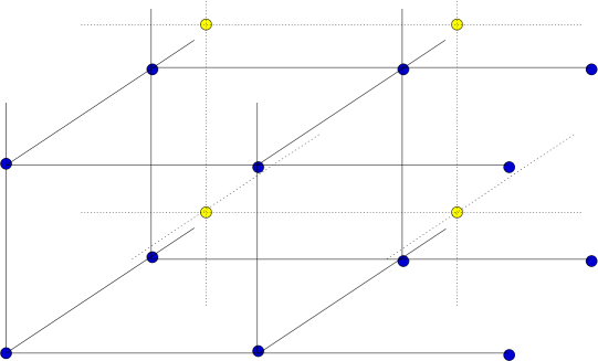
Figure 2: One ‘species’ of instantons lying at the midpoints of the lattice points of the other species of instantons.

In the special case $n=1$ (i.e. the caloron problem) one only needs $y_{1}-y_{2}$ to be parallel to $e_{0}$ for the quadratic term to vanish. This is a consequence of the fact that for $S^{1}\times{\mbox{\af R}}^{3}$ one may take $e_{0}$ and hence the elements of $\Lambda$ to be real. For $n>1$, $2(y_{1}-y_{2})\in\Lambda$ is a necessary   condition for the vanishing of the quadratic term. Thus for $2(y_{1}-y_{2})\notin\Lambda$ (4.9) is an approximation; (4.9) is then the first term of a power series expansion in the scale parameters.

Let us concentrate on the cases where the quadratic terms does vanish. Fourier transformation yields ${\tilde{\cal V}}^{-1}\hat{M}=-id_{z}-x+\hat{A}(z)$, where $\hat{A}(z)$ is the $SU(2)$ potential

$$\begin{array}[]{rcl}\displaystyle-i\hat{A}(z)=\left(\begin{array}[]{cc}\displaystyle\hbox{$\frac{1}{2}$}(y_{1}-y_{2})&\hbox{$\frac{1}{2}$}ie^{-i(y_{1}-y_{2})\cdot z}d_{z}\psi(z)Q\\ -\hbox{$\frac{1}{2}$}ie^{i(y_{1}-y_{2})\cdot z}d_{z}\psi(-z)Q&\hbox{$\frac{1}{2}$}(y_{2}-y_{1})\end{array}\right),\end{array}$$ (4.15)

and

$$\begin{array}[]{rcl}\displaystyle\psi(z)=\sum_{\alpha\in\Lambda}\frac{e^{i(\alpha+y_{1}-y_{2})\cdot z}}{|\alpha+y_{1}-y_{2}|^{2}}.\end{array}$$ (4.17)

$\psi(z)$ is a Green’s function for the Laplace operator on $\tilde{\mbox{\af T}}^{n}$

$$\begin{array}[]{rcl}\displaystyle d_{z}d_{z}^{*}\psi(z)=-{\tilde{\cal V}}e^{i(y_{1}-y_{2})\cdot z}\delta^{n}(z).\end{array}$$ (4.19)

Observe that $\psi$ is non-periodic

$$\begin{array}[]{rcl}\displaystyle\psi(z+\tilde{e}_{i})=e^{i(y_{1}-y_{2})\cdot\tilde{e}_{i}}\psi(z),\end{array}$$ (4.21)

where $\tilde{e}_{i}$ refers to the dual basis; $\tilde{e}_{i}\cdot e_{j}=2\pi\delta_{ij}$. Now if $2(y_{1}-y_{2})\in\Lambda$ and $(y_{1}-y_{2})\notin\Lambda$, $\psi(z)$ will be antiperiodic in at least one direction, and periodic in the remaining directions. One can also see that for these special values of $y_{1}-y_{2}$, $\psi(z)$ is real. The reality of $\psi$ is a sufficient condition for the potential (4.15) to be self-dual.

We now appear to have to deal with a non-Abelian Weyl operator. In what follows the inversion problem is reduced to an Abelian problem much like that for the one instanton case. Of course, in the light of the previous chapter due care regarding the meaning of the inverse is in order. ${\hat{M}}$ can be rewritten as follows

$$\begin{array}[]{rcl}\displaystyle{\tilde{\cal V}}^{-1}{\hat{M}}=e^{-\frac{i}{2}(y_{1}-y_{2})\cdot z\sigma_{3}}P^{-1}\left(\begin{array}[]{cc}\displaystyle D^{+}&0\cr 0&D^{-}\end{array}\right)Pe^{\frac{i}{2}(y_{1}-y_{2})\cdot z\sigma_{3}},\end{array}$$ (4.25)

where $D^{\pm}$ are the (Abelian) Weyl operators

$$\begin{array}[]{ccc}\displaystyle D^{\pm}=-id_{z}-x\pm\hbox{$\frac{1}{2}$}d_{z}\psi\,Q,&&\displaystyle P=\frac{1}{\sqrt{2}}(1\!\mbox{l}+i\sigma_{1}).\end{array}$$ (4.27)

The inverse of $\hat{M}$ is simply

$$\begin{array}[]{rcl}\displaystyle\hat{M}^{-1}(z,z^{\prime})={\tilde{\cal V}}e^{-\frac{i}{2}(y_{1}-y_{2})\cdot z\,\sigma_{3}}P^{-1}\Delta(z,z^{\prime})Pe^{\frac{i}{2}(y_{1}-y_{2})\cdot z^{\prime}\sigma_{3}},\end{array}$$ (4.29)

where $\Delta(z,z^{\prime})$ is a Green’s function for the diagonal operator $\hbox{diag}(D^{+},D^{-})$. Note that the exponentials in the decomposition of $\hat{M}^{-1}(z,z^{\prime})$ are not periodic. To ensure a periodic $\hat{M}^{-1}(z,z^{\prime})$ we must impose certain non-periodic boundary conditions on $\Delta(z,z^{\prime})$. Since we require $\hat{M}(z)\hat{M}^{-1}(z,z^{\prime})={\tilde{\cal V}}^{2}\delta^{n}(z-z^{\prime})$, then it follows that

$$\begin{array}[]{rcl}\displaystyle\left(\begin{array}[]{cc}\displaystyle D^{+}&0\cr 0&D^{-}\end{array}\right)\Delta(z,z^{\prime})=Pe^{\frac{i}{2}(z-z^{\prime})\cdot(y_{1}-y_{2})\sigma_{3}}P^{-1}\delta^{n}(z-z^{\prime}).\end{array}$$ (4.33)

It is convenient to absorb the exponential factor into the delta function. That is, consider the following (non-periodic) delta functions

$$\begin{array}[]{rcl}\displaystyle\delta_{1}^{n}(z)=e^{\frac{i}{2}z\cdot(y_{1}-y_{2})}\delta^{n}(z),\quad\delta_{2}^{n}(z)=e^{-\frac{i}{2}z\cdot(y_{1}-y_{2})}\delta^{n}(z).\end{array}$$ (4.35)

Using the following four (Abelian) Green’s functions, $\Delta^{\pm}_{i}(z,z^{\prime}),\quad i=1,2$, where

$$\begin{array}[]{rcl}\displaystyle D_{z}^{\pm}\Delta^{\pm}_{i}(z,z^{\prime})=\delta_{i}^{n}(z-z^{\prime}).\end{array}$$ (4.37)

$\Delta$ can be written as

$$\begin{array}[]{rcl}\displaystyle\Delta(z,z^{\prime})=\hbox{$\frac{1}{2}$}\left(\begin{array}[]{cc}\displaystyle\Delta^{+}_{1}+\Delta^{+}_{2}&i\left(\Delta^{+}_{1}-\Delta^{+}_{2}\right)\cr-i\left(\Delta^{-}_{1}-\Delta^{-}_{2}\right)&\Delta^{-}_{1}+\Delta^{-}_{2}\end{array}\right)(z,z^{\prime}).\end{array}$$ (4.41)

Accordingly

$$\begin{array}[]{rcl}\displaystyle\hat{M}^{-1}(z,z^{\prime})=\frac{{\tilde{\cal V}}}{2}e^{-\frac{i}{2}z\cdot(y_{1}-y_{2})\sigma_{3}}\left(\begin{array}[]{cc}\displaystyle\Delta^{+}_{1}+\Delta^{-}_{1}&-i\left(\Delta^{-}_{2}-\Delta^{+}_{2}\right)\cr i\left(\Delta^{-}_{1}-\Delta^{+}_{1}\right)&\Delta^{+}_{2}+\Delta^{-}_{2}\end{array}\right)(z,z^{\prime})e^{\frac{i}{2}z^{\prime}\cdot(y_{1}-y_{2})\sigma_{3}}.\\ \end{array}$$ (4.45)

4.2 Two-instanton on ${\mbox{\af T}}^{2}\times{\mbox{\af R}}^{2}$

Much as in section 3.2 we may take $e_{0}$ to be real and $e_{1}$ to be proportional to $Q$. Thus $\hat{Q}=Q/|Q|$ plays the same role as $\hat{l}$ did in the previous section. Indeed, the analogue of (3.16) is just $z=\hbox{$\frac{1}{2}$}\left(1-i\hat{Q}\right)\mbox{z}+\hbox{$\frac{1}{2}$}\left(1+i\hat{Q}\right)\bar{\mbox{z}}$. We can write the Abelian Dirac operators $D^{\pm}$ defined in (4.27) as follows

$$\begin{array}[]{rcl}\displaystyle D^{\pm}=e^{\mp\hbox{$\frac{1}{2}$}iQ\psi(z)}\left(-id_{z}-x_{||}\right)e^{\pm\hbox{$\frac{1}{2}$}iQ\psi(z)}-x_{\perp}.\end{array}$$ (4.47)

For the case $y_{2}-y_{1}=\hbox{$\frac{1}{2}$}(e_{0}+e_{1})$, we have

$$\begin{array}[]{rcl}\displaystyle\psi(z)=\frac{{\tilde{\cal V}}}{4\pi}\log\frac{\left|\theta\left(\frac{L_{0}}{4\pi}\mbox{z}+\frac{iL_{0}}{4L_{1}},\frac{iL_{0}}{2L_{1}}\right)\right|^{2}}{\left|\theta\left(\frac{L_{0}}{4\pi}\mbox{z}+\hbox{$\frac{1}{2}$},\frac{iL_{0}}{2L_{1}}\right)\right|^{2}},\end{array}$$ (4.49)

which is antiperiodic in both directions.

When $x_{\perp}=0$, the four Green’s functions $\Delta_{i}^{\pm}$ read

$$\Delta^{\pm}_{1}(z,z^{\prime}) \!\!= e^{\mp\hbox{$\frac{1}{2}$}iQ\psi(z)}\left[G_{1}(z-z^{\prime})\cosh\left(\hbox{$\frac{1}{2}$}|Q|\psi(z^{\prime})\right)\pm G_{2}(z-z^{\prime})i\hat{Q}\sinh\left(\hbox{$\frac{1}{2}$}|Q|\psi(z^{\prime})\right)\right]$$

$$\Delta^{\pm}_{2}(z,z^{\prime}) \!\!= e^{\mp\hbox{$\frac{1}{2}$}iQ\psi(z)}\left[G_{2}(z-z^{\prime})\cosh\left(\hbox{$\frac{1}{2}$}|Q|\psi(z^{\prime})\right)\pm G_{1}(z-z^{\prime})i\hat{Q}\sinh\left(\hbox{$\frac{1}{2}$}|Q|\psi(z^{\prime})\right)\right],$$

where the $G_{i}(z-z^{\prime})$ are (non-periodic) free Green’s functions defined as

$$\begin{array}[]{rcl}\displaystyle\left(-id_{z}-x_{||}\right)G_{i}(z-z^{\prime})=\delta_{i}^{2}(z-z^{\prime}),\quad i=1,2.\end{array}$$ (4.52)

Inserting (4.2) into (4.45) yields

$$\begin{array}[]{rcl}\displaystyle\hat{M}^{-1}(z,z^{\prime})={\tilde{\cal V}}\Psi(z)\left(\begin{array}[]{cc}\displaystyle G_{1}(z-z^{\prime})&0\cr 0&G_{2}(z-z^{\prime})\end{array}\right)\Psi^{-1}(z^{\prime}),\end{array}$$ (4.56)

where $\Psi(z)$ is the $2\times 2$ matrix

$$\begin{array}[]{rcl}\displaystyle\Psi(z)=\left(\begin{array}[]{cc}\displaystyle e^{-\hbox{$\frac{1}{2}$}i(y_{1}-y_{2})\cdot z}\cosh\left(\hbox{$\frac{1}{2}$}|Q|\psi(z)\right)&\hat{Q}e^{-\hbox{$\frac{1}{2}$}i(y_{1}-y_{2})\cdot z}\sinh\left(\hbox{$\frac{1}{2}$}|Q|\psi(z)\right)\cr-\hat{Q}e^{\hbox{$\frac{1}{2}$}i(y_{1}-y_{2})\cdot z}\sinh\left(\hbox{$\frac{1}{2}$}|Q|\psi(z)\right)&e^{\hbox{$\frac{1}{2}$}i(y_{1}-y_{2})\cdot z}\cosh\left(\hbox{$\frac{1}{2}$}|Q|\psi(z)\right)\end{array}\right).\end{array}$$ (4.60)

The two component row vector $n(z)$ is

$$\begin{array}[]{rcl}\displaystyle n(z)={\tilde{\cal V}}(q_{1}\,,\,q_{2})\Psi(0)\left(\begin{array}[]{cc}\displaystyle G_{1}(-z)&0\cr 0&G_{2}(-z)\end{array}\right)\Psi^{-1}(z).\end{array}$$ (4.64)

Again we encounter infinite constants; $\psi(z)\rightarrow\infty$ as $z\rightarrow 0$ and so all entries of the matrix $\Psi(0)$ are ‘infinite’. As in section 3.2 we will temporarily treat $\Psi(0)$ as a finite object. In the light of our one instanton calculation we expect some constraints on $q_{1}$ and $q_{2}$. We can choose $q_{1}$ to be real. In appendix B we show that for $n(z){n^{\dagger}(z)}$ to be integrable requires that

$$\begin{array}[]{rcl}\displaystyle(q_{1},\,\,\,q_{2})=\lambda(1,\,\,\,\hat{Q}),\end{array}$$ (4.66)

where $\lambda$ is a common scale parameter since $|q_{1}|=|q_{2}|=\lambda$. Observe that the relative group orientation of the two instantons is fixed. If the orientation of the first instanton lies at the ‘North pole’ of $S^{3}\equiv SU(2)$, then the orientation of the second instanton sits on the equator. Much as in the one instanton case the absence of non-integrable singularities leads to an upper bound on the scale parameter

$$\begin{array}[]{rcl}\displaystyle 0<\lambda^{2}{\tilde{\cal V}}<2\pi.\end{array}$$ (4.68)

Another consequence of (4.66) is that $(q_{1},\,\,q_{2})$ is an eigenvector of the infinite matrix $\Psi(0)$, i.e. $(q_{1},\,\,q_{2})\Psi(0)=e^{\hbox{$\frac{1}{2}$}|Q|\psi(0)}(q_{1},\,\,q_{2})$. As in the one instanton calculation we define a ‘finite’ row vector $\lambda{\tilde{\cal V}}n_{f}(z)=e^{-\hbox{$\frac{1}{2}$}|Q|\psi(0)}n(z)$. The final gauge potential is obtained by replacing $n(z)$ with $n_{f}(z)$ in (2.83) and replacing (2.85) with $\rho={\tilde{\cal V}}^{-1}\rho_{f}={\tilde{\cal V}}^{-1}\int_{\tilde{\mbox{\af T}}^{2}}n_{f}(z){n^{\dagger}_{f}(z)}.$

In the course of the construction a number of constraints have been put on the ADHM data. It is helpful to divide these constraints into two. The first constraints are simply those imposed by hand to achieve technical simplification, i.e. we imposed periodicity and the midpoint condition in order that we could exactly determine the Weyl operator. In addition to these constraints we were forced to impose the additional constraints (4.66) and (4.68). By virtue of the midpoint prescription and (4.66) our two instantons begin to resemble one instantons if we cut ${\mbox{\af T}}^{2}$ in half. In fact if we had chosen $y_{1}-y_{2}=\hbox{$\frac{1}{2}$}e_{0}$ or $y_{1}-y_{2}={1\over 2}e_{1}$ instead of $y_{1}-y_{2}=\hbox{$\frac{1}{2}$}(e_{0}+e_{1})$ then our ‘two instanton’ would be nothing more than a ‘doubled’ one instanton. That is one can always produce a two-instanton on ${\mbox{\af T}}^{n}\times{\mbox{\af R}}^{4-n}$ by taking a one instanton and doubling one of the periods. To show this equivalence one simply compares the ‘two instanton’ with $y_{1}-y_{2}=\hbox{$\frac{1}{2}$}e_{0}$ or $y_{1}-y_{2}=\hbox{$\frac{1}{2}$}e_{1}$ with the one instanton with $\omega={1\over 4}\tilde{e}_{0}$ or $\omega={1\over 4}\tilde{e}_{1}$. Then using the $q_{i}\rightarrow-q_{i}$ symmetry mentioned at the end of section 2.2 one can show that the two sets of ADHM data correspond to the same instanton. The two instanton corresponding to $y_{1}-y_{2}=\hbox{$\frac{1}{2}$}(e_{0}+e_{1})$ appears to be ‘genuine’ in the sense it is not equivalent to some one-instanton solution. However it seems plausible that the $y_{1}-y_{2}=\hbox{$\frac{1}{2}$}(e_{0}+e_{1})$ case corresponds to a twisted one instanton (the twisted Nahm transformation is discussed in [41]).

5 Discussion

In this paper we have described in a general way how to implement the ADHM construction of $SU(2)$ instantons on ${\mbox{\af T}}^{n}\times{\mbox{\af R}}^{4-n}$. The first step (which corresponds to solving the quadratic ADHM constraint) is to construct a self-dual $SU(k)$ ($U(1)$ for $k=1$) potential, $\hat{A}(z)$, on the dual torus $\tilde{\mbox{\af T}}^{n}$ (here $k$ is the topological charge). $\hat{A}(z)$ has singularities which are determined by the ADHM data (i.e. the scales, positions and group orientation of the ‘component’ instantons). We have constructed the Weyl operators corresponding to the general one-instanton and some two instantons on ${\mbox{\af T}}^{n}\times{\mbox{\af R}}^{4-n}$. However, the problem of solving the Weyl equations poses a considerable technical challenge. One is therefore motivated to start with lower values of $n$. We have considered the $n=2$ problem in some detail.

The solutions here are not deformations of ’t Hooft instantons; the ’t Hooft ansatz fails to provide solutions on ${\mbox{\af T}}^{2}\times{\mbox{\af R}}^{2}$. Unlike for $S^{1}\times{\mbox{\af R}}^{3}$ we are forced to impose constraints on the ADHM parameters in order to guarantee a well defined potential on ${\mbox{\af T}}^{2}\times{\mbox{\af R}}^{2}$. In particular, we find an upper bound on the scale parameters; for the one-instanton, $\lambda^{2}\tilde{\cal V}<4\pi$ and for our restricted two-instanton we found that $\lambda^{2}\tilde{\cal V}<2\pi$ (here we were forced to give the two component instantons a common scale parameter).

For $n>2$, i.e. ${\mbox{\af T}}^{3}\times{\mbox{\af R}}$ and ${\mbox{\af T}}^{4}$, the Weyl equations seem more problematic. While the ${\mbox{\af T}}^{2}\times{\mbox{\af R}}^{2}$ Weyl operator corresponds to an Aharonov-Bohm problem on $\tilde{\mbox{\af T}}^{2}$, on ${\mbox{\af T}}^{3}\times{\mbox{\af R}}$ we have to solve the Weyl equation on $\tilde{\mbox{\af T}}^{3}$ in the (self-dual) background of an electric and magnetic dipole field [42]. For ${\mbox{\af T}}^{4}$ the one instanton calculation should fail. Presumably there is no way to avoid non-integrable singularities. For our restricted two instantons the prospects seem a little brighter. This is because these seemingly correspond to twisted one instantons (or even $\frac{1}{2}$ instantons in the presence of non-orthogonal twists). There is no known obstacle to the existence of such objects on ${\mbox{\af T}}^{4}$.

Although the ${\mbox{\af T}}^{3}\times{\mbox{\af R}}$ and ${\mbox{\af T}}^{4}$ problems certainly merit more attention the ${\mbox{\af T}}^{2}\times{\mbox{\af R}}^{2}$ case requires further development. Even in the 1-instanton sector we were only able to provide closed forms for $A_{\mu}(x)$ and $F_{\mu\nu}(x)$ in a 2-dimensional subspace ($x_{\perp}=0$) of ${\mbox{\af T}}^{2}\times{\mbox{\af R}}^{2}$. To obtain analytic results for $x_{\perp}\neq 0$ requires progress in dealing with massive Aharonov-Bohm type Dirac equations on $\tilde{\mbox{\af T}}^{2}$. Furthermore, we have said nothing about the geometry of the moduli space or the constituent monopoles of our instantons. One could numerically plot the action density of the one instantons in the plane $x_{\perp}=0$ to see if there are two peaks associated with the two expected monopole constituents.

Appendix A The quadratic term in (2.42)

In this appendix we show that the quadratic term in (2.42) vanishes for the one instanton and particular two instanton described in chapter 4.

Let us start with the one instanton. The quadratic term in question is

$$\begin{array}[]{rcl}\displaystyle{\cal R}^{\alpha\beta}=\sum_{\gamma\in\Lambda}\left(b^{\gamma\alpha}{}^{*}b^{\gamma\beta}-b^{\gamma\beta}{}^{*}b^{\gamma\alpha}\right).\end{array}$$ (A.2)

Assuming ${\cal R}^{\alpha\beta}=0$ leads to (3.6). Inserting this into (A.2) gives

$$\begin{array}[]{rcl}\displaystyle{\cal R}^{\alpha\beta}&=&\displaystyle\!\!-\lambda^{4}\sum_{\gamma\in\Lambda\setminus\{\alpha,\beta\}}\hat{l}\left(\frac{1}{(\gamma-\alpha)^{*}}\frac{1}{\gamma-\beta}-\frac{1}{(\gamma-\beta)^{*}}\frac{1}{\gamma-\alpha}\right)\hat{l}\\ \displaystyle\hfil&&\displaystyle\ \ \ \ \ ~{}~{}~{}~{}~{}~{}~{}~{}~{}~{}~{}~{}~{}\times\sin\left[(\alpha-\gamma)\cdot\omega\right]\sin\left[(\beta-\gamma)\cdot\omega\right].\end{array}$$ (A.5)

It is clear that each summand in (A.5) does not separately vanish. Rather there is a pairwise cancellation; for each $\gamma\in\Lambda\setminus\{\alpha,\beta\}$ there is exactly one other lattice point $\gamma^{\prime}\in\Lambda\setminus\{\alpha,\beta\}$ so that the two summands add up to zero. It is apparent that the appropriate choice for $\gamma^{\prime}$ is $\gamma^{\prime}=-\gamma+\alpha+\beta.$ If $2\gamma=\alpha+\beta$, i.e. $\gamma^{\prime}=\gamma$, then the summand itself vanishes.

The argument is similar for the two instanton of section 4. Here the quadratic term is

$$\begin{array}[]{rcl}\displaystyle{\cal R}_{ij}^{\alpha\beta}=\sum_{\gamma\in\Lambda}\left(b_{1i}^{\gamma\alpha}{}^{*}b_{1j}^{\gamma\beta}-b_{1j}^{\gamma\beta}{}^{*}b_{1i}^{\gamma\alpha}+b_{2i}^{\gamma\alpha}{}^{*}b_{2j}^{\gamma\beta}-b_{2j}^{\gamma\beta}{}^{*}b_{2i}^{\gamma\alpha}\right).\end{array}$$ (A.7)

Inserting (4.9) gives ${\cal R}_{12}^{\alpha\beta}={\cal R}_{21}^{\alpha\beta}=0$, and

$${\cal R}_{22}^{\alpha\beta} = \sum_{\gamma\in\Lambda}\left(b_{12}^{\gamma\alpha}{}^{*}b_{12}^{\gamma\beta}-b_{12}^{\gamma\beta}{}^{*}b_{12}^{\gamma\alpha}\right)$$

$$= -\frac{1}{4}\sum_{\gamma\in\Lambda}\left(Q\frac{1}{\gamma-\alpha+y_{1}-y_{2}}\frac{1}{(\gamma-\beta+y_{1}-y_{2})^{*}}Q\right.$$

$$\left.~{}~{}~{}~{}~{}~{}~{}~{}~{}~{}~{}-Q\frac{1}{\gamma-\beta+y_{1}-y_{2}}\frac{1}{(\gamma-\alpha+y_{1}-y_{2})^{*}}Q\right).$$

Now we will show that ${\cal R}_{22}$ is zero for $2(y_{1}-y_{2})\in\Lambda$. As in the one instanton case each summand in (A) does not separately vanish. For each $\gamma\in\Lambda$ there is one other lattice point $\gamma^{\prime}\in\Lambda$ so that the two summands add up to zero

$$\begin{array}[]{rcl}\displaystyle\gamma^{\prime}=-\gamma+\alpha+\beta-2(y_{1}-y_{2}).\end{array}$$ (A.10)

Since $\gamma^{\prime}\in\Lambda$ we require $2(y_{1}-y_{2})\in\Lambda$. If $2\gamma=\beta+\alpha-2(y_{1}-y_{2})$ then $\gamma^{\prime}=\gamma$ so that we do not have two counterbalancing summands. However, in this case the summand itself vanishes.

Appendix B Equation (3.71)

In this appendix we outline a proof of (3.71) which, for $x_{\perp}=0$, is equivalent to the statement that $f(z,z^{\prime})$ commutes with the quaternions. In the caloron problem one simply notes that $f$ is the inverse of $M^{\dagger}M$ which by construction commutes with the quaternions. We could also explicitly check that our $f$ is the inverse of $M^{\dagger}M$. However, we would face the thorny problem of coincident fluxes and sources [43, 44, 45]. Therefore, we will adopt a more pedestrian approach. Before we embark on this we note that for $z+z^{\prime}=0$ a trivial change of variables in the integrals defining $g_{-}(z,z^{\prime})$ suffices to verify (3.71). For $z+z^{\prime}\neq 0$ we have a more indirect argument. When $z\neq\omega$ it is easy to check that

$$\left(-i\partial_{\bar{\hbox{z}}}-\hbox{$\frac{1}{2}$}\hbox{x}_{||}\right)e^{-2\lambda^{2}\phi(z)}\left(-i\partial_{\hbox{z}}-\hbox{$\frac{1}{2}$}\bar{\hbox{x}}_{||}\right)\left(g_{+}(z,z^{\prime})-e^{2\lambda^{2}\phi(z)}g_{-}(z,z^{\prime})e^{2\lambda^{2}\phi(z^{\prime})}\right)=0.$$ (B.1)

This shows that the left and right hand sides of (3.71) satisfy the same differential equations. To complete the argument we must show that they obey the same boundary conditions. Clearly both are periodic on $\tilde{\mbox{\af T}}^{2}$, but we also need to show that $g_{+}(z,z^{\prime})$ and $e^{2\lambda^{2}\phi(z)}g_{-}(z,z^{\prime})e^{2\lambda^{2}\phi(z^{\prime})}$ have the same asymptotics at the fluxes. Let us examine $g_{\pm}(z,z^{\prime})$ in the neighbourhood of $z=\omega$. One can see that $g_{+}(\omega,z^{\prime})$ is well defined for $\lambda^{2}\tilde{\cal V}<2\pi$, while $g_{-}(\omega,z^{\prime})=0$. This does not contradict (3.71) since the exponential $e^{2\lambda^{2}\phi(z)}$ diverges as $\kappa|\mbox{z}-\mbox{w}|^{-\lambda^{2}{\tilde{\cal V}}/(2\pi)}$ for $z\sim\omega$ where $\kappa$ is a constant. Consistency requires that $g_{-}(z,z^{\prime})\sim\kappa^{-1}|\mbox{z}-\mbox{w}|^{\lambda^{2}\tilde{\cal V}/(2\pi)}g_{+}(\omega,z^{\prime})e^{-2\lambda^{2}\phi(z^{\prime})}$ for $z\sim\omega$. One can show that $g_{-}(z,z^{\prime})$ decays as it should in the limit $z\rightarrow\omega$ by considering the derivative of $g_{-}(z,z^{\prime})$:

$$\!\!\left(-i\partial_{\bar{\mbox{z}}}-\hbox{$\frac{1}{2}$}\mbox{x}_{||}\right)g_{-}(z,z^{\prime}) = \!\hbox{$\frac{1}{2}$}e^{-2\lambda^{2}\phi(z)}G_{+}(z-z^{\prime})$$

$$\!-\frac{e^{-2\lambda^{2}\phi(z)}}{2\rho_{f}}G_{+}(-\omega+z)\int_{\tilde{\mbox{\af T}}^{2}}d^{2}y^{\prime}G_{-}(\omega-y^{\prime})e^{-2\lambda^{2}\phi(y^{\prime})}G_{+}(y^{\prime}-z^{\prime}).$$

In the neighbourhood of $z=\omega$, $2\pi G_{+}(-\omega+z)\sim i/(\bar{\mbox{z}}-\bar{\mbox{w}})$, and so the second term in (B) dominates (provided $z^{\prime}\neq\pm\omega$). Integrating yields

$$g_{-}(z,z^{\prime})\sim\frac{1}{\lambda^{2}\tilde{\cal V}\kappa\rho_{f}}|\mbox{z}-\mbox{w}|^{\lambda^{2}\tilde{\cal V}/(2\pi)}\int_{\tilde{\mbox{\af T}}^{2}}d^{2}y^{\prime}G_{-}(\omega-y^{\prime})e^{-2\lambda^{2}\phi(y^{\prime})}G_{+}(y^{\prime}-z^{\prime}),$$ (B.3)

which indeed decays correctly. Full agreement with (3.71) requires

$$g_{+}(\omega,z^{\prime})=\frac{e^{2\lambda^{2}\phi(z^{\prime})}}{\lambda^{2}\tilde{\cal V}\rho_{f}}\int_{\tilde{\mbox{\af T}}^{2}}d^{2}y^{\prime}G_{-}(\omega-y^{\prime})e^{-2\lambda^{2}\phi(y^{\prime})}G_{+}(y^{\prime}-z^{\prime}).$$ (B.4)

To check this one simply notes that away from $z^{\prime}=\pm\omega$ the left and right hand sides are annihilated by the same differential operator, $\left(i\partial_{\mbox{z}^{\prime}}-\hbox{$\frac{1}{2}$}\bar{\mbox{x}}_{||}-2i\lambda^{2}\partial_{\mbox{z}^{\prime}}\phi(z^{\prime})\right)\left(i\partial_{\bar{\mbox{z}}^{\prime}}-\hbox{$\frac{1}{2}$}\mbox{x}_{||}\right)$. It is simple to also check that they agree in the neighbourhoods of $z^{\prime}=\pm\omega$ which completes the proof.

Appendix C Two instanton singularities

Consider the 2-component row vectors $v_{\pm}=(1,\,\,\pm\hat{Q})$ which are (formally) eigenvectors of $\Psi(0)$ in that $v_{\pm}\Psi(0)=e^{\pm\hbox{$\frac{1}{2}$}|Q|\psi(0)}v_{\pm}$. We now make the decomposition $(q_{1},\,\,q_{2})=\alpha_{+}v_{+}+\alpha_{-}v_{-}$ where the quaternions $\alpha_{\pm}$ are not completely free since $q_{1}^{*}q_{2}-q_{2}^{*}q_{1}=Q$. The integrand in the definition of $\rho$ is

$${\tilde{\cal V}}^{-1}n(z){n^{\dagger}}(z) = |\alpha_{+}|^{2}e^{|Q|\psi(0)}\left[\mathcal{G}_{+}(-z){\mathcal{G}_{+}^{*}(z)}e^{-|Q|\psi(z)}+\mathcal{G}_{-}(-z){\mathcal{G}_{-}^{*}(z)}e^{|Q|\psi(z)}\right]$$

$$+|\alpha_{-}|^{2}e^{-|Q|\psi(0)}\left[\mathcal{G}_{+}(-z){\mathcal{G}_{+}^{*}(z)}e^{|Q|\psi(z)}+\mathcal{G}_{-}(-z){\mathcal{G}_{-}^{*}(z)}e^{-|Q|\psi(z)}\right]$$

$$+\hbox{terms linear in $\alpha_{+}\alpha_{-}^{*}$ and $\alpha_{-}\alpha_{+}^{*}$,}$$

where we have employed the notation

$$\mathcal{G}_{\pm}(z)=G_{1}(z)\pm G_{2}(z),$$ (C.2)

not to be confused with the $G_{\pm}(z)$ introduced in section 3.2! First, let us consider the singularity structure of the free Green’s functions $\mathcal{G}_{\pm}(z)$ which satisfy $(-id_{z}-x)\mathcal{G}_{\pm}(z)=\delta_{1}(z)\pm\delta_{2}(z).$ Now $\delta_{1}^{2}(z)$ and $\delta_{2}^{2}(z)$ are zero except for all dual lattice points ($z\in\tilde{\Lambda}$). However $\delta_{1}^{2}(z)+\delta_{2}^{2}(z)$ is only singular at half of the lattice points, while $\delta_{1}^{2}(z)-\delta_{2}^{2}(z)$ is singular at the remaining dual lattice points. This can be seen from the following identities

$$\delta_{1}^{2}(z)+\delta_{2}^{2}(z)=2\cos\left(\hbox{$\frac{1}{2}$}(y_{1}-y_{2})\cdot z\right)\delta^{2}(z),\quad\delta_{1}^{2}(z)-\delta_{2}^{2}(z)=2i\sin\left(\hbox{$\frac{1}{2}$}(y_{1}-y_{2})\cdot z\right)\delta^{2}(z).$$ (C.3)

Now since $2(y_{1}-y_{2})\in\Lambda$ it follows that $\hbox{$\frac{1}{2}$}(y_{1}-y_{2})\cdot z=\hbox{$\frac{1}{2}$}\pi n,\quad n\in{\mbox{\af Z}}$ for $z\in\tilde{\Lambda}$ which means that either the sine or the cosine must be zero for $z\in\tilde{\Lambda}$. In particular, we see that unlike $\delta_{1}^{2}(z)+\delta_{2}^{2}(z)$, $\delta_{1}^{2}(z)-\delta_{2}^{2}(z)$ has no singularity at $z=0$. Thus we conclude that $\mathcal{G}_{-}(z)$ has no singularity at $z=0$. In the neighbourhood of $z=0$ we have

$$\begin{array}[]{rcl}\displaystyle\mathcal{G}_{+}(-z){\mathcal{G}_{+}^{*}(z)}\propto\frac{1}{|\mbox{z}|^{2}},\quad\mathcal{G}_{-}(-z){\mathcal{G}_{-}^{*}(z)}\hbox{ non-singular.}\end{array}$$ (C.5)

We also require the behaviour of $\psi(z)$ at $z=0$, $\psi(z)\sim-({{\tilde{\cal V}}}/{2\pi})\log|\mbox{z}|$. Near $z=0$ we have

$$\begin{array}[]{rcl}\displaystyle\mathcal{G}_{+}(-z){\mathcal{G}_{+}^{*}(z)}e^{-|Q|\psi(z)}\propto|\mbox{z}|^{-2+|Q|{\tilde{\cal V}}/(2\pi)},\quad\mathcal{G}_{+}(-z){\mathcal{G}_{+}^{*}(z)}e^{|Q|\psi(z)}\propto|\mbox{z}|^{-2-|Q|{\tilde{\cal V}}/(2\pi)}.\\ \end{array}$$ (C.7)

The second part of (C.7), i.e. $\mathcal{G}_{+}(-z){\mathcal{G}_{+}^{*}(z)}e^{|Q|\psi(z)}$ is non-integrable. However, this term is absent in the $|\alpha_{+}|^{2}$ contribution to (C) and so if we make the choice $\alpha_{-}=0$ we do not encounter this singularity. The first part of (C.7) is an integrable singularity for $|Q|>0$. In fact if we take $|Q|{\tilde{\cal V}}>4\pi$ the singularity disappears. However, then $\mathcal{G}_{-}(-z){\mathcal{G}_{-}^{*}(z)}e^{|Q|\psi(z)}$ will become non integrable. Accordingly, for the singularities in (2.85) to be integrable we require $\alpha_{-}=0,$ and $0<|Q|{\tilde{\cal V}}<4\pi$ which implies (4.66) and (4.68).

References

- [1] A.A. Belavin, A.M. Polyakov, A.S. Schwarz and Yu. S. Tyupkin, Phys. Lett. B59 (1975) 85.
- [2] P. Goddard, P. Mansfield and H. Osborn, Phys. Lett. B 98 (1981) 59.
- [3] P. Mansfield, Nucl. Phys. B186 (1981) 287.
- [4] H. Osborn, Annals Phys. 135 (1981) 373.
- [5] D. Finnel and P. Pouliot, Nucl. Phys. B453 (1995) 225.
- [6] N. Dorey, V.V. Khoze and M.P. Mattis, Phys. Rev D54 (1996) 2921.
- [7] A. Yung, Nucl. Phys. B485 (1997) 38.
- [8] N. Seiberg and E. Witten, Nucl. Phys. B 426 (1994) 19, (E) B430 (1994) 485.
- [9] G. ’t Hooft, Comm. Math. Phys. 81 (1981) 455.
- [10] C. Taubes, J. Diff. Geom. 19 (1984) 517.
- [11] P.J. Braam and P. van Baal, Commun. Math. Phys. 122 (1989) 267.
- [12] P. van Baal, Nucl. Phys. Proc. Suppl. 49 (1996) 238.
- [13] J.-L. Richard and A. Rouet, Nucl. Phys. B 211 (1983) 447.
- [14] M.F. Atiyah, N.J. Hitchin, V.G. Drinfeld and Yu. I. Manin, Phys. Lett. A65, 185, 1978.
- [15] E.F. Corrigan and D.B. Fairlie, Phys. Lett. B 67 (1977) 69.
- [16] G. ’t Hooft, unpublished.
- [17] F. Wilczek, in ‘Quark Confinement and Field Theory’, edited by D. Stump and D. Weingarten, Wiley, New York (1977).
- [18] R. Jackiw, C. Nohl and C. Rebbi, Phys. Rev. D15 (1979) 1642.
- [19] E. Mottola and A. Wipf, Phys. Rev. D 39 (1989) 588.
- [20] W. Nahm, Phys. Lett. B 90 (1980) 413.
- [21] E. Corrigan and P. Goddard, Ann. Phys. (NY) 154 (1984) 253.
- [22] T. C. Kraan and P. van Baal, Nucl. Phys. B 533 (1998) 627.
- [23] T. C. Kraan and P. van Baal, Phys. Lett. B 435 (1998) 389.
- [24] K. Lee and C. Lu, Phys. Rev. D58 (1998) 025100.
- [25] H. Reinhardt, Nucl. Phys. B503 (1997) 505.
- [26] C. Ford, U. G. Mitreuter, J. M. Pawlowski, T. Tok, and A. Wipf, Ann. Phys. (NY) 269 (1998) 26.
- [27] C. Ford, T. Tok and A. Wipf, Nucl. Phys. B 548 (1999) 585.
- [28] O. Jahn and F. Lenz, Phys. Rev. D58 (1998) 085006.
- [29] L. S. Schulman, J. Math. Phys. 12 (1971) 304.
- [30] R. Sundrum and L.J. Tassie, J. Math. Phys. 27 (1986) 1566.
- [31] C. H. Oh, C.P. Soo and C.H. Lai, J. Math. Phys. 29 (1988) 1154.
- [32] A. Kapustin and S. Sethi, Adv. Theor. Math. Phys. 2 (1998) 571.
- [33] M. Jardim, ‘Construction of doubly-periodic instantons’, math.dg/9909069.
- [34] M. Jardim, ‘Spectral curves and Nahm transformation for doubly periodic instantons’, math.ag/9909146.
- [35] M. Jardim, ‘Nahm transformation for doubly periodic instantons’ math.dg/9910120.
- [36] S.A. Cherkis and A. Kapustin, ‘Nahm transformation for periodic monopoles and super Yang-Mills theory’, hep-th/0006050.
- [37] N.H. Christ, E.J. Weinberg and N.K. Stanton, Phys. Rev. D18 (1978) 2013.
- [38] E. Corrigan, D.B. Fairlie, P. Goddard and S. Templeton, Nucl. Phys. B140 (1978) 31.
- [39] B. J. Harrington and H. K. Shepard, Phys. Rev. D17 (1978) 2122.
- [40] D. Mumford, ‘Tata lectures on theta 1’, Birkhäuser, 1982.
- [41] A. Gonzalez-Arroyo, Nucl. Phys. B548 (1999) 626.
- [42] P. van Baal, Phys. Lett. B 448 (1999) 26.
- [43] P. Gerbert, Phys. Rev D40 (1989) 229.
- [44] R. Jackiw, ‘Delta function potentials in two and three dimensional quantum mechanics’, M. A. Bég Memorial Volume, eds. A. Ali and P. Hoodboy (1991) World Scientific.
- [45] L. Dabrowski and P. Stovicek, J. Math. Phys. 39 (1998) 47.