Confinement, asymptotic freedom and renormalons in type 0 string duals

Abstract:

Type 0B string theory has been proposed as the dual description of non-supersymmetric SU(N) Yang-Mills theory coupled to six scalars, in four dimensions. We study numerically and analytically the equations of motion of type 0B gravity and we find RG trajectories of the dual theory that flow from an asymptotically free UV regime to a confining IR regime. In the UV we find a one-parameter family of solutions that approach asymptotically $AdS_{5}\times S^{5}$ with a logarithmic flow of the coupling plus non-perturbative terms that correctly reproduce all UV and IR renormalon singularities. The first UV renormalon gives a contribution $\sim F_{1}(E)/E^{2}$ and we are able to predict also the form of the function $F_{1}(E)$, which, from the YM side, corresponds to summing all multiple-chain bubble graphs. The fact that the positions of the renormalon singularities in the Borel plane come out correctly is a non-trivial test of the conjectured duality.

1 Introduction and summary

The attempts to generalize the Maldacena conjecture [1, 2, 3, 4] to four-dimensional non-supersymmetric YM theories have followed different directions. The approach proposed by Witten is to start from the duality between type II strings and a five-dimensional super-YM; compactifying the fifth dimension on a circle with different boundary conditions for bosons and fermions one breaks supersymmetry and is left with an effective four-dimensional non-supersymmetric theory [5]. A conceptually similar possibility is to reduce the supersymmetry to $N=1$ or even $N=0$ with the addition of mass deformations [6, 7, 8].

A different strategy is to start directly from a string theory with worldsheet supersymmetry but no spacetime supersymmetry. Polyakov has advocated this approach and has suggested the use of non-critical strings [9, 10], and Klebanov and Tseytlin [11, 12] have adapted this suggestion to critical type 0B string theory. On the gravity side one considers a configuration of $N$ electric D3-brane in the type 0B theory, and the dual field theory is conjectured to be $SU(N)$ four-dimensional YM plus six adjoint scalars. The six scalars are the price to pay for working in the critical dimension.

In this paper we follow the latter approach and we study the renormalization group (RG) flow derived from the equations of motion of type 0B gravity. Klebanov and Tseytlin [12] have found that in the UV one recovers asymptotic freedom,

$$\frac{1}{g_{\rm YM}^{2}(E)}\sim\ln\frac{E}{\Lambda}-{\rm const.}\,\ln\ln\frac{E}{\Lambda}\,.$$ (1)

The numerical value of the beta function coefficients are not under control because of various corrections discussed below, but it is very encouraging to see the correct logarithmic behaviour. Minahan [13, 14] has instead presented confining IR solutions. Further related work appeared in refs. [15]-[20]. It is therefore natural to ask whether asymptotic freedom and confinement are connected by a single RG flow.

In this paper we perform a detailed analytic and numerical investigation of the RG flow, and we find the following results.

• The UV solution found in refs. [12, 14] is just a member of a one-parameter family of solutions. The free parameter $\kappa$, which is related to subleading terms in the UV, determines the IR behaviour of the solution. For $\kappa$ smaller than a critical value $\kappa_{c}$ (that we can determine analytically) the solution flows in the IR toward a confining solution. The case considered in [12] corresponds instead to $\kappa>\kappa_{c}$, and it was found in [12] that in this case the solution flows in the IR toward a conformal fixed point at infinite coupling.

• We will then show, both numerically and analytically, the existence of RG trajectories that connect asymptotic freedom in the UV with confinement in the IR.

• We will find that in the UV, beside the logarithmic terms shown in eq. (1), type 0B gravity predicts also power corrections,

  $$\frac{1}{g_{\rm YM}^{2}(E)}\sim\ln\frac{E}{\Lambda}-c_{1}\ln\ln\frac{E}{\Lambda}+c_{2}F_{1}(E)\frac{\Lambda^{2}}{E^{2}}+c_{3}F_{2}(E)\frac{\Lambda^{4}}{E^{4}}+c_{4}\frac{\Lambda^{4}}{E^{4}}+O(\frac{1}{E^{6}})$$ (2)

  where the $c_{i}$ are constants to be defined below. These power corrections match exactly the non-perturbative contributions coming from renormalons. The term $\sim F_{1}(E)/E^{2}$ on the field theory side comes from the first UV renormalon, the term $\sim F_{2}(E)/E^{4}$ from the second UV renormalon, and similarly we get the contributions of all UV renormalons. The term $c_{4}/E^{4}$ is the leading IR renormalon, and we correctly find no IR renormalon contribution $1/E^{2}$. Thus, we get the right positions of all renormalon singularities in the Borel plane.

• Even the energy dependence of the prefactors, that is $F_{1}(E)$ for the first UV renormalon and a constant for the leading IR renormalon, matches what is known from the field theory side. In particular, we will predict the energy dependence

  $$F_{1}(E)\sim\sin\left(\beta_{T}\ln\frac{E}{\Lambda}+\alpha_{T}\right)$$ (3)

  with $\alpha_{T},\beta_{T}$ constants. Expanding at first order in $\beta_{T}$ we get a result consistent with what is obtained in QCD summing diagrams with a single bubble chain. The above closed form is a prediction of the dual string theory for the resummation of multiple chain bubble graphs, which would be very interesting to check from the field theory side.

The above results hold at lowest order in $\alpha^{\prime}$ and string loop corrections, and are presented in sects. 3-6. The fact that some features of the UV limit of the YM theory can be obtained from the gravity side is surprising, since the $SU(N)$ YM and the gravity descriptions are duals to each other and are based on opposite expansions, in $g^{2}N$ and $1/\sqrt{g^{2}N}$, respectively. It is therefore important to study the corrections to the gravity predictions in the UV limit. We will discuss them in sect. 7. It has been found in ref. [12] that, if the $\alpha^{\prime}$ corrections can be expressed in terms of the Weyl tensor, then the only price to pay in the UV is that the numerical values of the beta function coefficients cannot be predicted, but the logarithmic running of the coupling is unaltered. Furthermore we will find that, under the same conditions, the position of the renormalon singularities in the Borel plane is independent of the $\alpha^{\prime}$ corrections.

2 General strategy for computing the RG flow

In this section we discuss the general strategy and the assumptions used to extract the RG flow in the dual theory from the gravity equations of motion of type 0 strings. The low energy effective action of type 0B strings [21, 22, 23] is written in terms of a (closed string) tachyon field $T$, the dilaton $\phi$, the metric, and a doubled set of RR fields. The terms involving the tachyon in the effective action have been discussed by Klebanov and Tseytlin [11], and are

$$\int d^{10}x\sqrt{G}e^{-2\phi}\left(\frac{1}{2}G^{mn}\partial_{m}T\partial_{n}T+V(T)\right)+\int d^{10}x\sqrt{G}\,\frac{1}{2}f(T)|F_{5}|^{2}\,.$$ (4)

Because of world-sheet supersymmetry, the tachyon potential $V(T)$ has only even powers of $T$. We write (to have the same notations of [14]) $V(T)=-2g(T)$, and

$$g(T)=-\frac{1}{4}m^{2}T^{2}-\lambda T^{4}+O(T^{6})=\frac{1}{2}T^{2}+O(T^{4})\,.$$ (5)

The tachyon mass is $m^{2}=-2/\alpha^{\prime}$ and we have set $\alpha^{\prime}=1$. The function $f(T)$ describes the coupling of the tachyon to the 5-form field strength $F_{5}$, and is given by

$$f(T)=1+T+\frac{1}{2}T^{2}+O(T^{3})$$ (6)

and the coupling to the other RR fields can be found in ref. [11]. Note that, due to the doubling of RR fields, the 5-form field strength is not constrained to be self-dual, so that $|F_{5}|^{2}$ is non vanishing. D-branes in this theory have been studied in [24, 11]. Another consequence of the doubling of the RR fields is that there are two kinds of D-branes, electrically and magnetically charged. It is then interesting to consider the solution of the gravity equations of motion corresponding to a large number $N$ of coinciding electrically charged 3-branes, since from eq. (4) we see that the coupling of the 3-brane to the 5-form RR field strength can stabilize the closed string tachyon. The tachyon from open strings which ends on parallel D-branes is instead eliminated by the GSO projection [11, 9]. In the Einstein frame, the ansatz for the 3-brane metric can be conveniently written in terms of two functions $\xi$ and $\eta$ of a transverse variable $\rho$,

$$ds_{E}^{2}=e^{\frac{\xi}{2}-5\eta}d\rho^{2}+e^{-\frac{\xi}{2}}dx_{(4)}^{2}+e^{\frac{\xi}{2}-\eta}d\Omega_{(5)}^{2}\,.$$ (7)

For the 4-form RR field $C_{(4)}$ one takes $C_{0123}(\rho)$ as the only non-vanishing component, so that $F_{5}=dC_{(4)}$ has only the component $(F_{5})_{0123\rho}$; similarly one takes $T=T(\rho),\phi=\phi(\rho)$. The equation of motion for the RR field can be explicitly integrated and gives an integration constant $Q$ which is just the RR charge, and is proportional to $N$. The remaining equations of motion then separate into four dynamical equations [11, 14]

$$\ddot{\phi}+\frac{1}{2}g(T)e^{\frac{\phi+\xi}{2}-5\eta}=0\,,$$ (8)

$$\ddot{\xi}+\frac{1}{2}g(T)e^{\frac{\phi+\xi}{2}-5\eta}+\frac{2Q^{2}}{f(T)}e^{-2\xi}=0\,,$$ (9)

$$\ddot{\eta}+\frac{1}{2}g(T)e^{\frac{\phi+\xi}{2}-5\eta}+8e^{-4\eta}=0\,,$$ (10)

$$\ddot{T}+\frac{2Q^{2}f^{\prime}(T)}{f^{2}(T)}e^{-2\xi}+2g^{\prime}(T)e^{\frac{\phi+\xi}{2}-5\eta}=0\,,$$ (11)

and (due to the invariance under reparametrizations of $\rho$) a constraint on the initial values, conserved by the dynamical equations,

$$\frac{{\dot{\phi}}^{2}}{2}+\frac{{\dot{\xi}}^{2}}{2}-5{\dot{\eta}}^{2}+\frac{{\dot{T}}^{2}}{4}+g(T)e^{\frac{\phi+\xi}{2}-5\eta}+20e^{-4\eta}-Q^{2}\frac{e^{-2\xi}}{f(T)}=0\,.$$ (12)

The dot is the derivative with respect to $\rho$. The explicit form of $f(T)$ plays an important role in the UV regime, where the tachyon is stabilized at its minimum, $f^{\prime}(T_{0})=0$ [11].

There are uncertainties due to the fact that neither $f(T)$ nor $g(T)$ are known in closed form; actually the latter is not even unambiguously defined, since, using the equations of motions, a term $\sim\nabla^{2}T$ in the effective action can be traded for a term $\sim m^{2}T$ so that, for instance, a higher derivative term $\sim(\nabla^{2}T)^{4}$ in the effective action can be reabsorbed into a $\sim T^{4}$ term. In the following we will at first set $g(T)=(1/2)T^{2}$ and $f(T)=1+T+T^{2}/2$ (the minimum of $f(T)$ is in this case at $T_{0}=-1$). We will then discuss how our results depend on these choices.

Our aim is to solve eqs. (8)–(12), and to translate the solutions into a renormalization group flow of the coupling $g_{\rm YM}^{2}$ of the dual theory. The first issue is how to read $g_{\rm YM}^{2}$ from the gravity side. We follow the approach of [13, 14, 12] and we read it from the quark-antiquark potential, computed from the Wilson loops as in refs. [25, 26]. This means that we take

$$g_{\rm YM}^{2}\sim\exp\{\phi(\rho)/2\}$$ (13)

as our definition of the coupling. The exact proportionality factor will not concern us here since, as found in refs. [14, 12] and as we will discuss below, the gravity solution is in any case subject to a number of uncertainties, due to $\alpha^{\prime}$ corrections and to the exact form of $f(T),g(T)$, that affect the numerical value of the proportionality coefficient in eq. (13).

The definition (13) is apparently in contradiction with what one would obtain from the D-brane effective action, which seems to give $g_{\rm YM}^{2}\sim\exp\{\phi\}$ rather than $\sim\exp\{\phi/2\}$. However, as discussed in [12], in the type 0 theory there exists also a tachyon tadpole on the D-brane, so that the effective action of the D-brane is proportional not simply to $e^{-\phi}$ but rather to $k(T)e^{-\phi}$, with $k(T)=1+T/4+O(T^{2})$. Since in the UV the tachyon runs toward its minimum at $T_{0}=-1$, higher powers in $k(T)$ cannot be neglected and the closed form of $k(T)$ is needed to draw conclusions. It is clear, however, that this is a point which deserves further investigations.

Eq. (13) provides us with the dependence of the coupling on the transverse coordinate $\rho$. To obtain an RG flow, the second step is to connect $\rho$ with a physical energy scale. This can be done as follows. From eq. (7) we see that a dilatation of the 4-dimensional coordinates, $x\rightarrow\lambda x$, can be reabsorbed into a rescaling of $\xi$ such that $\exp\{-\xi/2\}$ scales like an energy squared (while rescaling $\eta$ and $\rho$ so to keep the other terms invariant). We will then define the energy scale from $\exp\{-\xi(\rho)/2\}\sim E^{2}$, or

$$\ln\frac{E}{\Lambda}=-\frac{1}{4}\xi(\rho)\,.$$ (14)

$\Lambda$ is a scale that we will determine later. In the UV region the solutions will approach $AdS_{5}\times S^{5}$ and, writing the metric of $AdS_{5}$ as $\sim du^{2}/u^{2}+u^{2}dx_{(4)}^{2}$, we see that $\exp(-\xi/2)\sim u^{2}$ and then the prescription (14) reduces to the by now standard identification $u\sim E$. Far from the UV there is a certain arbitrariness in this definition, that we regard as corresponding to the arbitrariness in the choice of the renormalization scheme on the gauge theory side. Of course the details of the beta function are not independent of these choices, and only universal properties, like the existence of zeros and how the zeros are approached are what really matters.

Solving the equations of motion we get $\phi(\rho)$ and $\xi(\rho)$. Combining eqs. (13) and (14) then provides the dependence of $g_{\rm YM}^{2}$ from the energy scale and therefore the RG flow.

3 The UV and IR asymptotics

An asymptotic solution valid in the UV limit has been presented in ref. [14] and, as a more systematic expansion, in ref. [12]. Direct inspection of eqs. (8)–(12) reveals however that there is actually a one-parameter family of solutions. It is convenient to introduce a new variable $y$ from

$$\rho\equiv e^{-y}\,.$$ (15)

In the limit $y\rightarrow\infty$ the solution is

$$\phi = -2\ln y+15\ln 2+\frac{1}{y}(39\ln y+\kappa)+O\left(\frac{\ln^{2}y}{y^{2}}\right)\,,$$ (16)

$$\xi = -y+\ln 2+\frac{1}{y}+\frac{1}{2y^{2}}(39\ln y+\kappa-104)+O\left(\frac{\ln^{2}y}{y^{3}}\right)\,,$$ (17)

$$\eta = -\frac{y}{2}+\ln 2+\frac{1}{y}+\frac{1}{2y^{2}}(39\ln y+\kappa-38)+O\left(\frac{\ln^{2}y}{y^{3}}\right)\,,$$ (18)

$$T = -1+\frac{8}{y}+\frac{4}{y^{2}}(39\ln y+\kappa-20)+O\left(\frac{\ln^{2}y}{y^{3}}\right)\,.$$ (19)

Here and in the following we set $Q=1$; we see from the equations that the solution for generic $Q$ can be recovered from

$$\xi(y;Q) = \xi(y;Q=1)+\ln Q\,,$$

$$\phi(y;Q) = \phi(y;Q=1)-\ln Q\,,$$ (20)

while $\eta,T$ are independent of $Q$; $\kappa$ is a free parameter, and the solution found in ref. [12] corresponds to $\kappa=0$. In spite of the fact that in the UV $\kappa$ only appears in terms which look quite subleading, we will find that its value is very important for determining the IR behaviour of the solution. In the large $y$ limit $\xi\sim-y\rightarrow-\infty$. Eq. (14) then shows that $y\rightarrow\infty$ (or $\rho\rightarrow 0$) is the UV region. At $y=\infty$ the metric reduces to $AdS_{5}\times S^{5}$.

Using the prescription discussed in sect. 2, one can now extract the RG flow in the UV, with the result [12]

$$g_{\rm YM}^{2}(E)\sim\frac{1}{\ln(E/\Lambda)-\frac{39}{8}\ln\ln(E/\Lambda)}\,.$$ (21)

Note that the logarithmic terms are independent of $\kappa$. Eq. (21) should be compared to the running of the coupling in the proposed dual theory, that is four-dimensional $SU(N)$ YM theory with 6 scalars in the adjoint representation, which at the two-loop level is

$$g_{\rm YM}^{2}(E)=\frac{8\pi^{2}}{b_{1}\left(\ln(E/\Lambda)+\frac{b_{2}}{2b_{1}^{2}}\ln\ln(E/\Lambda)\right)}$$ (22)

with

$$b_{1}=\frac{8}{3}N\,,\hskip 42.67912pt\frac{b_{2}}{2b_{1}^{2}}=-\frac{3}{16}\,.$$ (23)

We see that eq. (21) qualitatively reproduces the logarithmic running of the coupling in the UV. The precise value of the beta function coefficients cannot be reliably estimated, since the gravity prediction is affected by $\alpha^{\prime}$ corrections (see refs. [12, 14] and sect. 7). Furthermore, with a generic tachyon potential $g(T)$, and a generic function $f(T)$ with a minimum at $T=T_{0}$, the factor $39/8$ in eq. (21) is modified as [14]

$$\frac{39}{8}\rightarrow\frac{7}{8}+\left(\frac{g^{\prime}(T_{0})}{g(T_{0})}\right)^{2}\,,$$ (24)

so it is clear that the values of the numerical coefficients are not under control.

In the opposite limit, $\rho\rightarrow\infty$, it is again possible to find asymptotic solutions. In this case however there is a much larger variety of solutions. In particular Minahan [14] has considered the generic behaviour

$$\phi \simeq \phi_{1}\rho+\phi_{0}\,$$

$$\xi \simeq \xi_{1}\rho+\xi_{0}\,$$ (25)

$$\eta \simeq \eta_{1}\rho+\eta_{0}\,$$

$$T \simeq t_{1}\rho+t_{0}\,,$$

At large $\rho$ this is a solution of the equations of motion if

$$\xi_{1},\eta_{1}>0\,,\hskip 14.22636pt5\eta_{1}-\frac{1}{2}\phi_{1}-\frac{1}{2}\xi_{1}>0$$ (26)

and

$$\frac{1}{2}\phi_{1}^{2}+\frac{1}{2}\xi_{1}^{2}-5\eta_{1}^{2}+\frac{1}{4}t_{1}^{2}=0\,.$$ (27)

The latter equation follows from the constraint equation (12), while the inequalities (26) ensure that all exponentials in eqs. (8)–(12) are suppressed and therefore that the equations of motions are satisfied.

In the limit $\rho\rightarrow\infty$ we now have $\xi\rightarrow+\infty$ and eq. (14) tells that this is the IR limit. To investigate confinement one can compute the quark-antiquark potential as in ref. [25, 26, 27, 28]. One considers a Wilson loop on the boundary $\rho=0$, with edges along the directions $x,t$, and looks for the classical string world-sheet $\rho(x,t)$ which has the Wilson loop as its boundary. The Nambu-Goto action is

$$S_{NG}=\frac{1}{2\pi\alpha^{\prime}}\int d\sigma d\tau\sqrt{\det(G_{MN}\partial_{\alpha}X^{M}\partial_{\beta}X^{N})}\,,$$ (28)

where $G_{MN}$ is the string frame metric, which in ten dimensions is related to the Einstein frame metric $G_{MN}^{(E)}$ by $G_{MN}=e^{\phi/2}G_{MN}^{(E)}$, and $G_{MN}^{(E)}$ for the 3-brane solution is given in eq. (7). Inserting $G_{MN}$ into eq. (28) one finds that the static potential $V(L)$ of a $q\bar{q}$ pair separated by a distance $L$ along the direction $x$ is obtained from [14]

$$V(L)=\frac{1}{2\pi\alpha^{\prime}}\int_{0}^{L}dx\,\left[e^{\phi-5\eta}\left(\frac{\partial\rho}{\partial x}\right)^{2}+e^{\phi-\xi}\right]^{1/2}\,,$$ (29)

after subtracting the divergent part corresponding to the energy of two separated massive quarks [25, 4]. The above result holds for generic $Q$. The $Q$ dependence can be extracted using eq. (3) and gives

$$V(L)=\frac{1}{2\pi\alpha^{\prime}\sqrt{Q}}\int_{0}^{L}dx\,\left[[e^{\phi-5\eta}]_{Q=1}\left(\frac{\partial\rho}{\partial x}\right)^{2}+\frac{1}{Q}[e^{\phi-\xi}]_{Q=1}\right]^{1/2}\,.$$ (30)

The result depends crucially on the function

$$\tilde{f}^{2}(\rho)\equiv[e^{\phi-\xi}]_{Q=1}\,\stackrel{{\scriptstyle\rho\rightarrow\infty}}{{\longrightarrow}}e^{(\phi_{1}-\xi_{1})\rho+(\phi_{0}-\xi_{0})}\,.$$ (31)

(We define $\phi_{0},\xi_{0}$ as the coefficient of the solution with $Q=1$). If $\phi_{1}<\xi_{1}$, $\tilde{f}$ vanishes at $\rho=\infty$, and the classical string configuration will go all the way to the region where $\rho\rightarrow\infty$, where there is no cost in energy in separating the quarks further; for $\phi_{1}=\xi_{1}$, the classical string configuration again goes to the minimum of $\tilde{f}(\rho)$ at $\rho\rightarrow\infty$, but now $\tilde{f}(\infty)=\exp\{(\phi_{0}-\xi_{0})\}$ is non-vanishing; the $q\bar{q}$ potential at large $L$ then becomes

$$V(L)\simeq\sigma L\,,$$ (32)

with

$$\sigma=\frac{1}{2\pi\alpha^{\prime}Q}\,e^{(\phi_{0}-\xi_{0})/2}$$ (33)

If instead $\phi_{1}>\xi_{1}$, then the function $\tilde{f}(\rho)$ diverges at $\rho\rightarrow\infty$. On the other hand, it also diverges in the UV, where $(\phi-\xi)\rightarrow y\rightarrow+\infty$, see eqs. (16)–(17). This means that it has a minimum at some value $\rho_{\rm min}$, where the classical string configuration goes. Then we have again a linear $q\bar{q}$ potential with

$$\sigma=\frac{1}{2\pi\alpha^{\prime}Q}\,\tilde{f}(\rho_{\rm min};Q=1)\,.$$ (34)

This gives the relation between the ‘QCD’ string tension $\sigma$, the type 0 string tension $1/(2\pi\alpha^{\prime})$ and the RR charge $Q$. In the case of $SU(3)$ YM, the experiment gives $\sigma\sim(1\,{\rm fm})^{-2}$ and eqs. (33) or (34) fix the value of $\alpha^{\prime}$ for the dual string theory.

Summarizing, the condition for confinement is

$$\phi_{1}\geq\xi_{1}\,.$$ (35)

A very different IR solution has been found by Klebanov and Tseytlin [12]. In this case, approaching the IR limit, the Einstein frame metric becomes again asymptotic to $AdS_{5}\times S^{5}$, while the dilaton diverges and the tachyon goes to zero. Therefore the dual theory flows toward a conformally invariant point with infinite coupling.

It is at this point natural to ask whether the one-parameter family of UV solutions discussed before is smoothly connected to any of these IR solutions. This is the issue that we will address in the next section numerically and in sect. 5 analytically.

4 Numerical integration

The numerical study of eqs. (8)–(11) is not as straightforward as one might hope; actually we found that, if we start from the UV with initial conditions that reproduce the asymptotic behaviour given by eqs. (16)–(19), the numerical integration runs almost immediately into divergencies. The reason for this numerical problem will become clear at the end of this section, but we have found that starting instead from the IR with a solution of the type (25) and integrating toward the UV poses no numerical problem.

However, this class of IR solutions from which we are starting the integration is characterized by more free parameters than the solution (16)-(19) to which we would like to connect in the UV. This means that we have to scan the parameter space of the IR solutions in order to find those very particular solutions (if any) that match to the desired UV behaviour. This can be done as follows. We start by studying an IR ($\rho\gg 1$) solution of the asymptotic form

$$\phi(\rho)=\rho\,,\hskip 14.22636pt\xi(\rho)=\rho\,,\hskip 14.22636pt\eta(\rho)=\frac{1}{\sqrt{5}}\rho+\eta_{0}\,,\hskip 14.22636ptT(\rho)=0\,,$$ (36)

keeping $\eta_{0}$ as the only free parameter. This is a solution of the type (25), where we have chosen $\phi_{1}=\xi_{1}$ in order to have a confining solution, see eq. (35), and we have arbitrarily set $\xi_{1}=1$. We also specialize to solutions such that in the IR the tachyon goes to zero. Eq. (27) then fixes $\eta_{1}=1/\sqrt{5}$. The inequalities (26) are satisfied. The invariance under constant shifts in $\rho$ allows to fix, e.g., $\xi_{0}=0$. We also set $\phi_{0}=0$; from eq. (33) we see that a different value of $\phi_{0}$ reflects itself on a quantitatively different value of the string tension $\sigma$, but we expect that this does not give rise to qualitative differences in the solution (as we have indeed checked numerically, setting $\eta_{0}=0$ and using $\xi_{0}$ as a free parameter).

The results of the numerical integration are as follows. For $\eta_{0}$ smaller than a critical value $\eta_{c}$, we find that $\eta(\rho)\rightarrow-\infty$ at a finite value of $\rho=\rho_{0}$, which therefore sets a limit to the range of $\rho$. The fact that $\rho$ cannot range from $-\infty$ to $+\infty$ is to be expected. In the usual Dp-brane solutions $\rho$ is indeed defined only in a semi-infinite range which, after a constant shift of $\rho$, can always be taken to be $0\leq\rho<\infty$, and $\rho=0$ is the D-brane horizon. However, in our case we find that $\xi(\rho_{0})$ is still finite. Since $\xi$ is related to the energy scale, $\xi=-4\ln(E/\Lambda)$, this means that in these solutions there is no region that we can interpret as an UV limit of the dual theory (or, in the gravity language, these solutions have no horizon). Therefore the solutions that start in the IR with $\eta_{0}<\eta_{c}$ are not connected to any of the UV solutions given by eqs. (16)–(19).

If instead $\eta_{0}>\eta_{c}$, the situation is reversed and $\xi\rightarrow-\infty$ at a finite value $\rho_{0}$ while $\eta(\rho_{0})$ and $\phi(\rho_{0})$ are still finite. This means that at $\rho_{0}$ the energy scale $E\rightarrow\infty$, so now the solution reaches the UV regime. However, $\phi(\rho_{0})$ is finite and therefore $g_{\rm YM}^{2}$ does not go to zero in the UV. Then, again, this IR solution does not match to the desired UV solution.

The situation is however different for $\eta_{0}=\eta_{c}$. In this case $\phi,\xi$ and $\eta$ all go toward $-\infty$ at the same value $\rho=\rho_{0}$, while $T\rightarrow-1$; therefore, there are chances of matching this solution with the UV solution of eqs. (16)–(19).

It is convenient to introduce the variable $y$ in analogy to eq. (15), so that the UV corresponds to $y\rightarrow\infty$. In the analytic computation of sect. (3) the UV limit was at $\rho=0$ while now it is at $\rho=\rho_{0}$, and to have the same convention we must make a constant shift in $\rho$ by $-\rho_{0}$, so we define $y$ from

$$\rho-\rho_{0}=e^{-y}\,.$$ (37)

With repeated runs we have located accurately the value of $\eta_{c}$ and the corresponding $\rho_{0}$, obtaining $\eta_{c}=0.4962700(1),\rho_{0}=-0.2076889(1)$. Locating $\eta_{c}$ with great precision is of course necessary if we want to follow the solution deep into the UV regime. With a precision $O(10^{-7})$ on $\eta_{c}$ we estimate that we can reliably follow the solution in the UV region up to $y\sim 7\ln 10=O(10)$.

The solution is shown in figs. (1)-(4) (solid lines), plotted against $y$. The functions $\xi,\eta$ and $T$ in the UV are very well fitted by the leading terms of eqs. (17), (18) and (19), suggesting that we have succeeded in matching the confining IR solution to this solution. For the dilaton, however, the situation is more subtle. Fig. (5) shows $e^{-\phi/2}\sim 1/g_{\rm YM}^{2}$ plotted against $-\xi/4$, i.e. against $\ln(E/\Lambda)$. In the IR the coupling is strong and $g_{\rm YM}^{2}\sim 1/E^{2}$, while in the UV regime $1/g_{\rm YM}^{2}$ scales linearly with $\ln E$.

Thus, first of all we see that we indeed succeeded in matching a confining IR solution with an asymptotically free UV regime, and now we want to understand whether this UV solution is related to eq. (16). If one compares with the data shown in fig. (2) one finds that, numerically, the expansion given by eq. (16) misses badly. It is instructive to understand the reason. In the UV region the numerical result is very well fitted by

$$e^{-\phi/2}\simeq A+by+O(\ln y)\,,$$ (38)

and the fit gives $b\simeq 0.005$. Thus, the solution in the UV is well reproduced by

$$\phi\simeq-2\ln\left(A+by+O(\ln y)\right)\,.$$ (39)

At asymptotically large values of $y$, this is the same as

$$\phi\simeq-2\ln y-2\ln b+O(\ln y/y)+O(1/y)\,.$$ (40)

This is just the leading behaviour predicted by eq. (16), which also predicts $b=2^{-15/2}\simeq 0.0055$, in excellent agreement with the value from the fit.

However, the expansion of $\ln(A+by)$ is valid only if $by\gg A$, and here $A$ is of order one while $b\simeq 0.0055$ is quite small. So, while eq. (39) reproduces the data very well, its expansion, and therefore eq. (16), is only valid for $y\gg 1/b\simeq 181$, which is well beyond the point where we can push the numerical integration. Then, it should be clear that our numerical solution in the UV is indeed nothing but a member of the family of solutions given in eqs. (16)–(19), and that the analytic expansion for $\phi$ given in eq. (16) is only valid for $y\gg 181$, rather than for $y\gg 1$. However, to clear up any doubt, in the next section we will present an improved analytic solution of the equations that is valid for $y\gg 1$, rather than only for $y\gg 181$, that in the region $y\gg 181$ reproduces eq. (16), including all the subleading terms written there, and that in the region $y<10$ where the numerical integration is possible reproduces very well the data. An unexpected bonus from this analysis will be that we will also find terms $\sim\exp\{-{\rm const.}y\}$, that we will relate in sect. (6) to renormalon singularities.

The physics of the solution is illustrated by figs. (5)-(7). Fig. (5), as already discussed, shows $\exp\{-\phi/2\}$, which is proportional to the inverse coupling $1/g_{\rm YM}^{2}$, as a function of $\ln(E/\Lambda)$. This plot can also be used to define the constant $\Lambda$ which fixes the energy scale. We define it as the value of $E$ when asymptotic freedom sets in, so by definition in fig. (5) the change of regime takes place at $\ln(E/\Lambda)=0$. On the right we have asymptotic freedom, since $1/g_{\rm YM}^{2}\sim\ln(E/\Lambda)$, while on the left side of the plot we have strong coupling and confinement.

Fig. (6) shows the beta functions $\beta(g_{\rm YM})$ for our solution. It has no zero except for the perturbative one at $g_{\rm YM}=0$, in contrast with the two-loop result, which has a second zero at $1/g_{\rm YM}^{2}=N/(4\pi)^{2}$, of course well outside the limit of validity of the perturbative computation, since there the ’t Hooft coupling is $Ng_{\rm YM}^{2}=(4\pi)^{2}\gg 1$. The numerical result in the intermediate region matches well the analytic results at weak and strong coupling.

Another interesting quantity is the radius of the 5-sphere (in the Einstein frame, since in this frame the UV metric approaches $AdS_{5}\times S^{5}$) $R_{(5)}$, which is given by eq. (7),

$$R_{(5)}^{2}=e^{\frac{\xi}{2}-\eta}\,.$$ (41)

If the adjoint scalar fields become massive, the radius of the 5-sphere shrinks to zero. We see from fig. (7) that $R_{(5)}^{2}$ diverges in the IR limit. At the transition between the IR and UV region it bounces and finally settles to the constant value $1/\sqrt{2}$ predicted by eqs. (17) and (18). We see that it never vanishes, and therefore the 6 adjoint scalars remain massless.

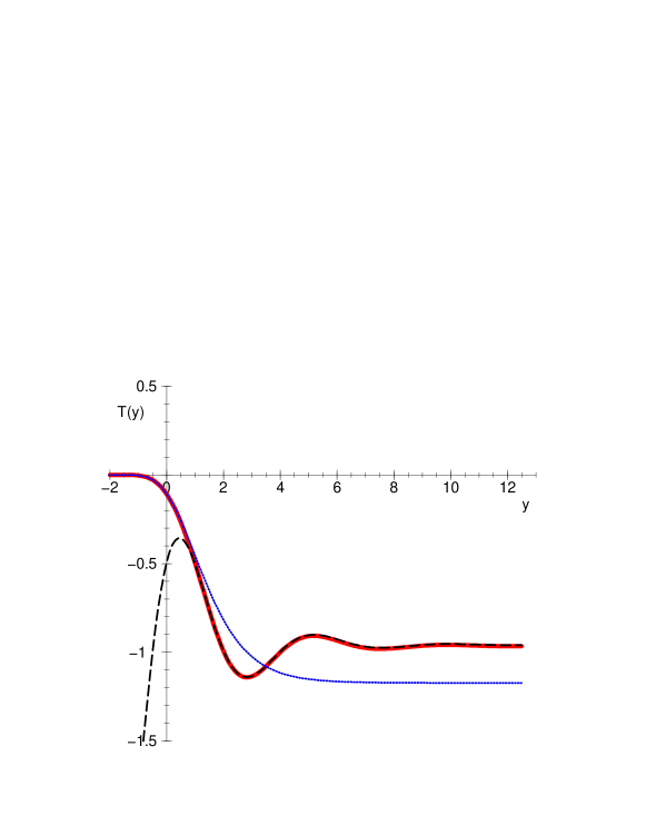
Figure 1: The result of the numerical integration for $T(y)$ (red solid line) discussed in sect. (4), together with the analytic results in the UV (black, dashed) and in the IR (blue, dotted) discussed in sect. 5.

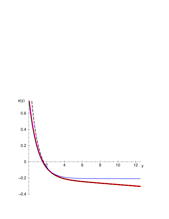
Figure 2: The result of the numerical integration for $\phi(y)$ (red solid line) discussed in sect. (4), together with the analytic results in the UV (black, dashed) and in the IR (blue, dotted) discussed in sect. 5.

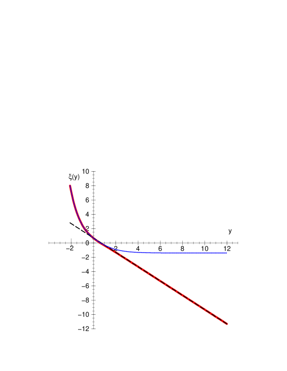
Figure 3: The result of the numerical integration for $\xi(y)$ (red solid line) discussed in sect. (4), together with the analytic results in the UV (black, dashed) and in the IR (blue, dotted) discussed in sect. 5.

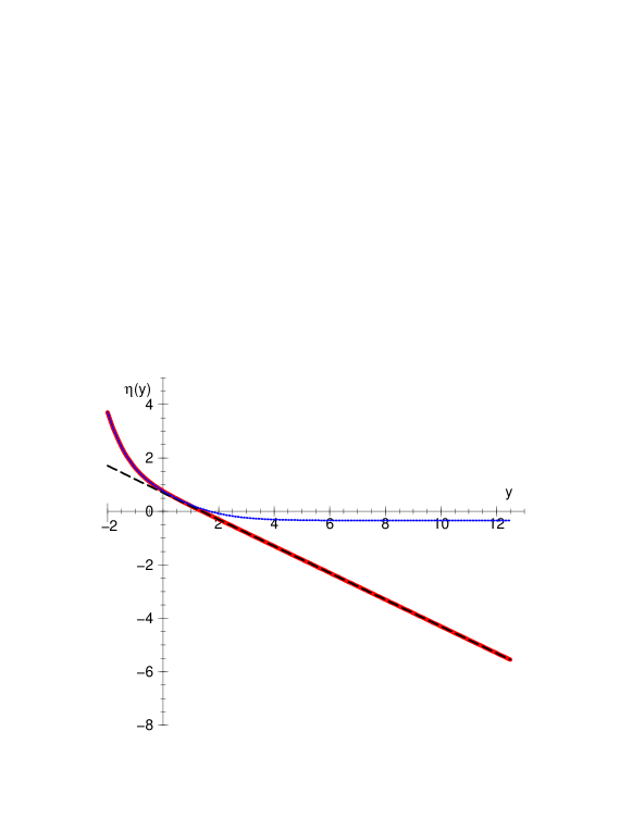
Figure 4: The result of the numerical integration for $\eta(y)$ (red solid line) discussed in sect. (4), together with the analytic results in the UV (black, dashed) and in the IR (blue, dotted) discussed in sect. 5.

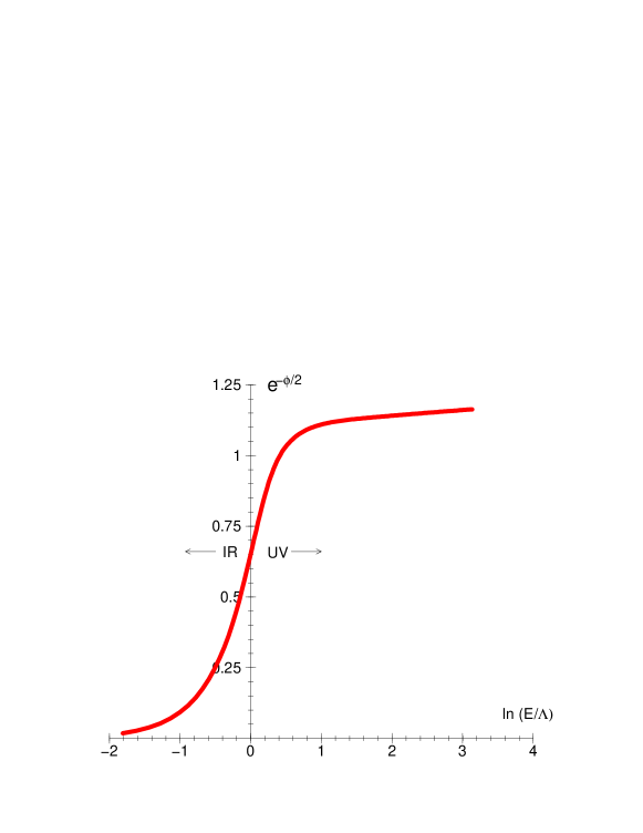
Figure 5: $e^{-\phi/2}$ (which is proportional to $1/g_{\rm YM}^{2}$) against $-\xi/4=\ln(E/\Lambda)$.

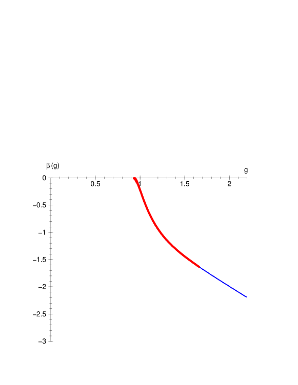
Figure 6: The beta function against $g_{\rm YM}$: numerical integration (red solid line), and IR analytic limit (blue, dotted). The UV analytic limit is $\beta(g)\sim-g^{3}$, and cannot be distinguished from zero on this vertical scale.

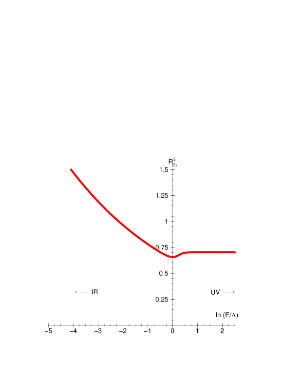
Figure 7: $R_{(5)}^{2}$ against $\ln(E/\Lambda)$.

5 Analytic solution

In this section we find an analytic expression for the RG flow which reproduces very well the solution from the IR to the UV regions, and even allows to compute exponentially small corrections in the UV limit.

The results of the previous section suggest the following improved UV ansatz

$$e^{-\phi/2} = A+by+u(y)\,$$ (42)

$$\xi(y) = -y+\ln 2+\zeta(y)\,$$ (43)

$$\eta(y) = -\frac{y}{2}+\ln 2+\omega(y)\,$$ (44)

$$T(y) = -1+t(y)\,.$$ (45)

where $u,\zeta,\omega$ and $t$ are small, in a sense that will be clarified below. Here $b=2^{-15/2}\simeq 1/181$, and $A$ is a constant of order one, yet to be fixed ($A>0$ otherwise the solution would not make sense when $by<-A$). At first, we linearize the equations of motion with respect to $u,\zeta,\omega$ and $t$ (we will discuss later the non-linear terms), and we get

$$\zeta^{\prime\prime}+\zeta^{\prime}-2\zeta \simeq -\frac{2b}{A+by}\left[1+\frac{\zeta}{2}-5\omega-2t-\frac{u}{A+by}\right]\,,$$ (46)

$$\omega^{\prime\prime}+\omega^{\prime}-2\omega \simeq -\frac{2b}{A+by}\left[1+\frac{\zeta}{2}-5\omega-2t-\frac{u}{A+by}\right]\,,$$ (47)

$$t^{\prime\prime}+t^{\prime}+2t \simeq +\frac{16b}{A+by}\left[1+\frac{\zeta}{2}-5\omega-t-\frac{u}{A+by}\right]\,,$$ (48)

$$u^{\prime\prime}+\left(1-\frac{2b}{A+by}\right)u^{\prime}+\frac{b^{2}}{(A+by)^{2}}u\simeq\frac{b^{2}}{A+by}+b(\frac{\zeta}{2}-5\omega-2t)\,.$$ (49)

where the prime is $d/dy$. We can now take advantage of the fact that $b$ is numerically small, and we treat it as a small expansion parameter. Instead $A+by$ in the UV is at least of order one. Then, to lowest order in $b$ a particular solution of eqs. (46)–(48) is given simply by

$$\zeta(y)=\omega(y)=\frac{1}{8}t(y)=\frac{b}{A+by}\left[1+O\left(\frac{b}{A+by}\right)\right]\,.$$ (50)

In fact, in the region where $A+by=O(1)$, $\zeta^{\prime}$ is smaller by a factor $b$ compared to $\zeta$ while for $y>>1/b$ we have $1\gg\zeta\sim 1/y\gg\zeta^{\prime}$, and similar for $\omega,t$. Substituting eq. (50) into eq. (49) we obtain the particular solution

$$u(y)=-\frac{39}{2}b\ln(A+by)\left[1+O\left(\frac{b}{A+by}\right)\right]\,,$$ (51)

To obtain the most general solution, we first tentatively assume that the terms $\sim\zeta,\omega,t$ and $\sim u/(A+by)$ on the right-hand side of eqs. (46)–(49) can be neglected compared to 1. Then the most general solution is obtained adding to the above particular solution the solution of the homogeneous equations

$$\zeta^{\prime\prime}+\zeta^{\prime}-2\zeta \simeq 0\,,\hskip 42.67912pt\omega^{\prime\prime}+\omega^{\prime}-2\omega\simeq 0\,,$$

$$t^{\prime\prime}+t^{\prime}+2t \simeq 0\,,\hskip 42.67912ptu^{\prime\prime}+u^{\prime}=0\,.$$ (52)

This would give

$$\zeta(y) \stackrel{{\scriptstyle?}}{{=}} \frac{b}{A+by}\left[1+O\left(\frac{b}{A+by}\right)\right]+B_{\xi}e^{-2y}\,,$$ (53)

$$\omega(y) \stackrel{{\scriptstyle?}}{{=}} \frac{b}{A+by}\left[1+O\left(\frac{b}{A+by}\right)\right]+B_{\eta}e^{-2y}\,,$$ (54)

$$t(y) \stackrel{{\scriptstyle?}}{{=}} \frac{8b}{A+by}\left[1+O\left(\frac{b}{A+by}\right)\right]+B_{T}e^{-y/2}\sin\left(\frac{\sqrt{7}}{2}y+\alpha_{T}\right)\,,$$ (55)

$$u(y) \stackrel{{\scriptstyle?}}{{=}} -\frac{39}{2}b\ln(A+by)\left[1+O\left(\frac{b}{A+by}\right)\right]+B_{u}e^{-y}\,,$$ (56)

where $B_{\xi},B_{\eta},B_{T},B_{u}$ and $\alpha_{T}$ are arbitrary coefficients of the homogeneous solutions. Note that the homogeneous equation for the tachyon has two complex solutions $t=\exp\{(-1\pm i\sqrt{7})y/2\}$, and then the solution is an oscillating function, as indeed we expected from fig. (1).

However, if we now insert back $\zeta,\omega,t$ and $u/(A+by)$ on the right-hand side of eqs. (46)–(49) to check whether the approach is self-consistent, we see that the tachyon gives a contribution $\sim bB_{T}e^{-y/2}\sin((\sqrt{7}/2)y+\alpha_{T})$ to the right-hand side of eqs. (46)–(49), so that, for instance, the term $e^{-2y}$ in the solution for $\zeta$ dominates over this contribution only if $be^{-y/2}\ll e^{-2y}$ or $y\ll\ln(1/b)$. In the opposite limit $y\gg\ln(1/b)$ (which with our value of $b$ means $y\gg 3$) before considering terms $\sim B_{\xi}e^{-2y}$ we must also include the contribution of the exponentially small term coming from $t$ to the right-hand side of eqs. (46)–(49), and we must also go beyond the linear approximation: e.g., if we want to get correctly all the terms up to $e^{-2y}$ we must include the contributions from terms $\sim t^{2},t^{3},t^{4}$ and $u^{2}$. The correct result then turns out to be of the form

$$e^{-\phi(y)/2} = A+by-\frac{39}{2}b\ln(A+by)\left[1+O\left(\frac{b}{A+by}\right)\right]+$$

$$+ b\,B_{T}e^{-y/2}\sin\left(\frac{\sqrt{7}}{2}y+\alpha_{T}\right)\left[1+O\left(bg_{1}(y)\right)\right]+$$

$$+ \left[B_{u}+bB_{T}^{2}g_{2}(y)\right]e^{-y}+O\left(e^{-3y/2}\right)\,,$$

with $g_{1}(y),g_{2}(y)$ non-singular and oscillating functions of $y$. In this work, we are not particularly interested in their explicit form (for the comparison with the numerical data these terms play a very marginal role), so we computed explicitly only the term $\sim e^{-y/2}$, at lowest order in $b$, but it is important conceptually to understand the structure of the exponentially small corrections, as we will see in sect. (6).

A similar structure can be obtained for $\xi,\eta,T$,

$$\xi(y) = -y+\ln 2+\frac{b}{A+by}\left[1+O\left(\frac{b}{A+by}\right)\right]$$

$$-\frac{bB_{T}}{A+by}e^{-y/2}\sin\left(\frac{\sqrt{7}}{2}y+\alpha_{T}\right)\left[1+O\left(\frac{b}{A+by}\right)\right]+O(e^{-y})\,,$$

$$\eta(y) = -\frac{y}{2}+\ln 2+\frac{b}{A+by}\left[1+O\left(\frac{b}{A+by}\right)\right]$$

$$-\frac{bB_{T}}{A+by}e^{-y/2}\sin\left(\frac{\sqrt{7}}{2}y+\alpha_{T}\right)\left[1+O\left(\frac{b}{A+by}\right)\right]+O(e^{-y})\,,$$

$$T(y) = -1+\frac{8b}{A+by}\left[1+O\left(\frac{b}{A+by}\right)\right]+$$

$$+B_{T}e^{-y/2}\sin\left(\frac{\sqrt{7}}{2}y+\alpha_{T}\right)\left[1+O\left(\frac{b}{A+by}\right)\right]+O\left(e^{-y}\right)\,.$$

We can now compare with the numerical solution and extract $A,B_{T},B_{u},\alpha_{T}$ from a fit. We find $A\simeq 1.1,B_{T}\simeq 0.8,B_{u}\simeq-0.6,\alpha_{T}\simeq 0.6$. This analytic solution is shown in figs. (1-4) (black dashed line) and we see that it reproduces very well the numerical solution already for $y\raise 1.72218pt\hbox{$>$}\kern-6.99997pt\lower 2.6694pt\hbox{$\sim$}1$.

Expanding eqs. (5)–(5) in the UV we find that they reproduce eqs. (16)–(19), including all subleading terms. The coefficient $\kappa$ is related to $A$ by

$$\kappa=39\ln b-\frac{2A}{b}=-\frac{585}{2}\ln 2-256\sqrt{2}\,A\,,$$ (61)

As we noted above, our solution makes sense only for $A>0$, since otherwise $\ln(A+by)$ becomes imaginary at intermediate values of $y$. Eq. (61) then shows that there exists a critical value of $\kappa$,

$$\kappa_{c}=-\frac{585}{2}\ln 2$$ (62)

and that our solution (5)-(5) can produce, in the deep UV region $y\gg 1/b$, only solutions of the form (16)-(19) with $\kappa<\kappa_{c}$. The solution considered by Klebanov and Tseytlin [12] has instead $\kappa=0$ and it does not belong to this class. Indeed, ref. [12] finds that in the IR it connects to another conformal fixed point at infinite coupling, rather than to a confining solution.

We see therefore that $\kappa$ plays a crucial role in determining the IR behaviour of the RG flow. In the language of Wilson’s renormalization group, this means that $\kappa$ is a parameter that determines to which universality class the UV theory belongs, and we have found that there are (at least) two universality classes: for $\kappa<\kappa_{c}$ we are in the domain of attraction of a confining IR fixed point, while for $\kappa>\kappa_{c}$ we are in the domain of attraction of a different fixed point.

It is also important to understand how the result changes if we change the form of the function $f(T)$. We find that, as long as $f(T)$ has a minimum at a finite value $T_{0}$, the qualitative behaviour of the solution does not change. However, it is especially important to known whether the exponential terms $\sim e^{-y/2}$ are affected by the form of $f(T)$. Linearizing eq. (11) for $f(T)$ generic, and writing $T=T_{0}+t$, the left-hand side of eq. (48) becomes $t^{\prime\prime}+t^{\prime}+ct$, with $c=f^{\prime\prime}(T_{0})/(2f^{2}(T_{0}))$; for $f(T)=1+T+T^{2}/2$, $c=2$. The homogeneous equation now has the solutions $t=e^{\gamma y}$ with

$$\gamma=-\frac{1}{2}(1\pm i\sqrt{4c-1})\,.$$ (63)

We see that, as long as $c\geq 1/4$, Re $\gamma$ is unchanged and we still have solutions of the form $e^{-y/2}\sin(\nu y)$, but the frequency $\nu$ depends on the explicit form of $f(T)$. Therefore the value that we found, $\nu=\sqrt{7}/2$, does not have a special significance, being related to the unknown form of $f(T)$, while the factor $e^{-y/2}$ is universal as long as $f(T)$ obeys

$$2f^{\prime\prime}(T_{0})\geq f^{2}(T_{0})\,.$$ (64)

The function $g(T)$ instead does not enter the homogeneous equation, so from this point of view its form is irrelevant.

Finally, it is straightforward to compute analytically the corrections to the solution in the IR regime. The corrections are exponentially small in $\rho$,

$$\phi= \phi_{1}\rho+\phi_{0} -\sum_{i=1}C_{i}^{(\phi)}\exp\{-\gamma_{i}^{(\phi)}\rho\}\,,$$

$$\xi= \xi_{1}\rho+\xi_{0} -\sum_{i=1}C_{i}^{(\xi)}\exp\{-\gamma_{i}^{(\xi)}\rho\}\,,$$ (65)

$$\eta= \eta_{1}\rho+\eta_{0} -\sum_{i=1}C_{i}^{(\eta)}\exp\{-\gamma_{i}^{(\eta)}\rho\}\,,$$

$$T= -\sum_{i=1}C_{i}^{(T)}\exp\{-\gamma_{i}^{(T)}\rho\}\,.$$

We have computed the coefficients $C_{i},\gamma_{i}$ for $i=1,2,3$. We get, for $\phi_{1}=\xi_{1}=\sqrt{5}\eta_{1}$,

$$\gamma_{1}^{(\phi)}=(\sqrt{5}+3)\phi_{1}\qquad\gamma_{2}^{(\phi)} = 2(\sqrt{5}+1)\phi_{1}\qquad\gamma_{3}^{(\phi)}=\frac{9+3\sqrt{5}}{\sqrt{5}}\phi_{1}$$

$$\gamma_{1}^{(\xi)}=2\phi_{1}\qquad\gamma_{2}^{(\xi)} = 4\phi_{1}\qquad\gamma_{3}^{(\xi)}=(\sqrt{5}+3)\phi_{1}$$

$$\gamma_{1}^{(\eta)}=\frac{4}{\sqrt{5}}\phi_{1}\qquad\gamma_{2}^{(\eta)} = \frac{8}{\sqrt{5}}\phi_{1}\qquad\gamma_{3}^{(\eta)}=(\sqrt{5}+3)\phi_{1}$$

$$\gamma_{1}^{(T)}=2\phi_{1}\qquad\gamma_{2}^{(T)} = (\sqrt{5}+1)\phi_{1}\qquad\gamma_{3}^{(T)}=4\phi_{1}$$

$$C_{1}^{(\phi)} = \frac{1}{16(\sqrt{5}+3)^{2}\phi_{1}^{6}}e^{\frac{1}{2}\phi_{0}-\frac{7}{2}\xi_{0}-5\eta_{0}}\qquad C_{2}^{(\phi)}=-\frac{1}{16(\sqrt{5}+1)^{4}\phi_{1}^{8}}e^{\phi_{0}-3\xi_{0}-10\eta_{0}}$$

$$C_{3}^{(\phi)} = \frac{125}{32(9+3\sqrt{5})^{2}\phi_{1}^{8}}e^{\frac{1}{2}\phi_{0}-\frac{7}{2}\xi_{0}-9\eta_{0}}\qquad C_{1}^{(\xi)}=\frac{1}{2\phi_{1}^{2}}e^{-2\xi_{0}}$$

$$C_{2}^{(\xi)} = \frac{3}{16\phi_{1}^{4}}e^{-4\xi_{0}}\qquad C_{3}^{(\xi)}=-\frac{1}{(\sqrt{5}+3)^{2}\phi_{1}^{6}}\left(\frac{2}{(\sqrt{5}+1)^{2}}-\frac{1}{16}\right)e^{\frac{1}{2}\phi_{0}-\frac{7}{2}\xi_{0}-5\eta_{0}}$$

$$C_{1}^{(\eta)} = \frac{5}{2\phi_{1}^{2}}e^{-4\eta_{0}}\qquad C_{2}^{(\eta)}=\frac{25}{4\phi_{1}^{4}}e^{-8\eta_{0}}$$

$$C_{3}^{(\eta)} = \frac{1}{16(\sqrt{5}+3)^{2}\phi_{1}^{6}}e^{\frac{1}{2}\phi_{0}-\frac{7}{2}\xi_{0}-5\eta_{0}}\qquad C_{1}^{(T)}=\frac{1}{2\phi_{1}^{2}}e^{-2\xi_{0}}$$

$$C_{2}^{(T)} = -\frac{1}{(\sqrt{5}+1)^{2}\phi_{1}^{4}}e^{\frac{1}{2}\phi_{0}-\frac{3}{2}\xi_{0}-5\eta_{0}}\qquad C_{3}^{(T)}=\frac{3}{16\phi_{1}^{4}}e^{-4\xi_{0}}$$

This analytic solution is shown in figs. (1-4) as a blue dotted line, and we see that it reproduces very well the numerical solution in the IR region. Having included the the first three subleading exponential, we see that the IR analytic solution has an overlap with the analytic UV solution, so that the two expansions together describe analytically the solution in the whole region.

6 The renormalon singularities

A striking feature of the UV solution is the appearance of the exponentially small terms $\sim e^{-y/2},e^{-y}$, etc.; in the UV, at leading order, $y\simeq-\xi=4\ln E$, so (extracting an overall proportionality factor $4b$) eq. (5) gives

$$\frac{1}{g_{\rm YM}^{2}(E)}\sim\ln\frac{E}{\Lambda}-\frac{39}{8}\ln\ln\frac{E}{\Lambda}+\frac{B_{T}}{4}F_{1}(E)\frac{\Lambda^{2}}{E^{2}}+B_{T}^{2}F_{2}(E)\frac{\Lambda^{4}}{E^{4}}+C\frac{\Lambda^{4}}{E^{4}}+O(\frac{1}{E^{6}})$$ (66)

with

$$F_{1}(E)=\sin\left(\beta_{T}\ln\frac{E}{\Lambda}+\alpha_{T}\right)\,\left[1+O(b)\right]\,,$$ (67)

and $C=B_{u}/(4b)$ (however, we expect that the numerical values of these coefficients will be affected by our uncertainties, as it happens to the factor $39/8$). $F_{2}(E)$ can be determined adding the terms $\sim t^{2}$ to eqs. (46) and (49). The positive constant $\beta_{T}$ is given by

$$\beta_{T}=2\left[\frac{2f^{\prime\prime}(T_{0})}{f^{2}(T_{0})}-1\right]^{1/2}\,,$$ (68)

and depends on the explicit form of $f(T)$, so its numerical value is not under control. The exponential correction to the relation $y\simeq-\xi$ gives an $O(b)$ contribution to (67).

First of all, we read from eq. (66) that there are power corrections, and they are exactly of the form that is expected from the effect of renormalons.

Let us recall that, given a divergent series

$$G(g_{\rm YM}^{2})=\sum_{n=1}^{\infty}G_{n}g_{\rm YM}^{2n}\,,$$ (69)

with $|G_{n}|$ bounded by $r^{n}n!$ at large $n$, one defines its Borel transform $B(z)$ as

$$B(z)=\sum_{n=0}^{\infty}\frac{G_{n+1}}{n!}z^{n}\,,$$ (70)

inside its convergence radius, $|zr|<1$, and by analytic continuation elsewhere. Then

$$G(g_{\rm YM}^{2})=\int_{0}^{\infty}dz\,e^{-z/g_{\rm YM}^{2}}B(z)\,$$ (71)

(where the integration contour is on the positive real axis) can provide a resummation of the perturbative series, depending on the structure of the singularities of $B(z)$ in the complex plane (Borel plane), and on the convergence properties of the integral at infinity. For asymptotically free non abelian gauge theories a number of singularities in the Borel plane have been identified as follows [29, 30, 31, 32]. IR renormalons give singularities on the positive semiaxis, at

$$\bar{z}=\frac{2}{\beta_{0}}k\,,\hskip 42.67912ptk=2,3,\ldots$$ (72)

($\beta_{0}>0$ for asymptotic freedom; in our case $\beta_{0}=\frac{8}{3}N/(8\pi^{2})$, see eq. (23)). Since these singularities are on the positive semiaxis, we must supplement eq. (71) with a prescription for dealing with them, and this produces non-perturbative contributions of order

$$\exp\{-\frac{2k}{\beta_{0}g_{\rm YM}^{2}}\}\sim\frac{1}{E^{2k}}\,,$$ (73)

times regular functions of the energy. Since the first IR renormalon is at $k=2$, it gives a contribution $\sim 1/E^{4}$. UV renormalons are instead on the negative semiaxis, at

$$\bar{z}=-\frac{2}{\beta_{0}}k\,,\hskip 42.67912ptk=1,2,3,\ldots$$ (74)

Even if these singularities are not on the integration contour, they limit the convergence radius of the expansion for $B(z)$ and are responsible for effects of the form

$$\exp\{-\frac{|\bar{z}|}{g_{\rm YM}^{2}}\}\sim\frac{1}{E^{2k}}$$ (75)

However, now $k$ starts from 1, so that the leading effect is $1/E^{2}$. There are further singularities on the positive semiaxis due to instantons, but their effect is of order $\exp(-8\pi^{2}/g_{\rm YM}^{2})$, which for $SU(N)$ with 6 adjoint scalars is $\sim(1/E)^{8N/3}$ (or $\sim(1/E)^{16N/3}$ if the first non-vanishing contribution comes from an instanton-antiinstanton pair) and therefore is quite suppressed for large $N$.

Comparing our result (66) with the above situation, we see that the $1/E^{2}$ term that we have found matches with the contribution of the first UV renormalon. The fact that we get the correct location of the renormalon singularity in the Borel plane is non-trivial, and can be traced back to the fact that the linearization of eq. (11) gave eq. (48), which has the homogeneous solution $t(y)=e^{\gamma y}$ with Re $\gamma=-1/2$, as long as eq. (64) holds. From the point of view of the gravity computation, we could have obtained $1/E^{\alpha}$ with $\alpha$ a priori any real number, not necessarily integer nor rational. We therefore regard this agreement as a successful and non trivial test of the conjectured duality between type 0B theory and non supersymmetric YM theory.

The term $B_{T}^{2}F_{2}(E)/E^{4}$ comes from the iteration of the term $B_{T}F_{1}(E)/E^{2}$, as we see from the coefficient $B_{T}^{2}$, so it clearly corresponds to the UV renormalon with $k=2$. Iterating further the contribution of the tachyon in the solution of the equations of motion, we find all the UV renormalons at their correct locations in the Borel plane.

The term $C/E^{4}$ instead has a prefactor which is just equal to the constant $C$ and is not related to $F_{1}(E)$ or $B_{T}$, so it has a different physical origin. Thus, we identify it with the $k=2$ IR renormalon. Again, it is very remarkable that its position in the Borel plane matches exactly the position of the first ($k=2$) IR renormalon; furthermore, we correctly find no term corresponding to an IR renormalon with $k=1$, which corresponds to the absence of gauge-invariant operators of dimension 2 in the OPE of current-current correlation functions.

Finally, even the energy dependence of the prefactors is consistent with what is known about renormalons from the analysis of Feynman graphs. In fact, in the approximation in which only a single chain of bubbles is considered, it is known that all UV renormalons are double poles, while the $k=2$ IR renormalon is a single pole, and all others IR renormalons are again double poles [32]. For a single pole

$$B(z)\sim\frac{1}{z-\frac{4}{\beta_{0}}},$$ (76)

and then eq. (71) gives a contribution $\sim\exp\{-4/(\beta_{0}g_{\rm YM}^{2})\}\sim 1/E^{4}$ without any further energy dependence, in full agreement with our interpretation of $C/E^{4}$ as the contribution of the $k=2$ IR renormalon. For a double pole on the positive semiaxis, instead, the non-perturbative contribution is of order

$$G(g_{\rm YM}^{2}) \sim \int_{0}^{\infty}dz\,e^{-z/g_{\rm YM}^{2}}\frac{1}{(z-\bar{z})^{2}}\rightarrow$$ (77)

$$\rightarrow \frac{1}{g_{\rm YM}^{2}}\int_{0}^{\infty}dz\,e^{-z/g_{\rm YM}^{2}}\frac{1}{(z-\bar{z})}\sim\frac{1}{g_{\rm YM}^{2}}e^{-\bar{z}/g_{\rm YM}^{2}}\,,$$

where in the second line we have integrated by parts and kept only the non-analytic term. This provides a $\ln E$ term in the prefactor. Similarly, there are logarithmic terms from the double poles on the negative semiaxis [32, 33]. Thus in the single chain approximation the first UV renormalon is of order

$$\sim\frac{\beta_{0}\ln E}{E^{2}}\,,$$ (78)

and in our approach is reproduced by the first term of the expansion of eq. (67) in powers of $\beta_{T}$ (which suggests that $\beta_{T}$ is proportional to $\beta_{0}$). Higher order terms are expected to come from graphs with multiple chains insertions, and are not well understood in QCD [32]. In this sense, eq. (67) is also a remarkable prediction of the dual string theory, that would be very interesting to check from the YM side.

At low energies $F_{1}(E)$ oscillates faster and faster, see (fig. 8). This is physically very reasonable, since these oscillations signal the transition from asymptotic freedom to the confining regime. Thus, the form of $F_{1}(E)$ seems to capture both the correct single chain result and a physically correct behaviour when the IR is approached.

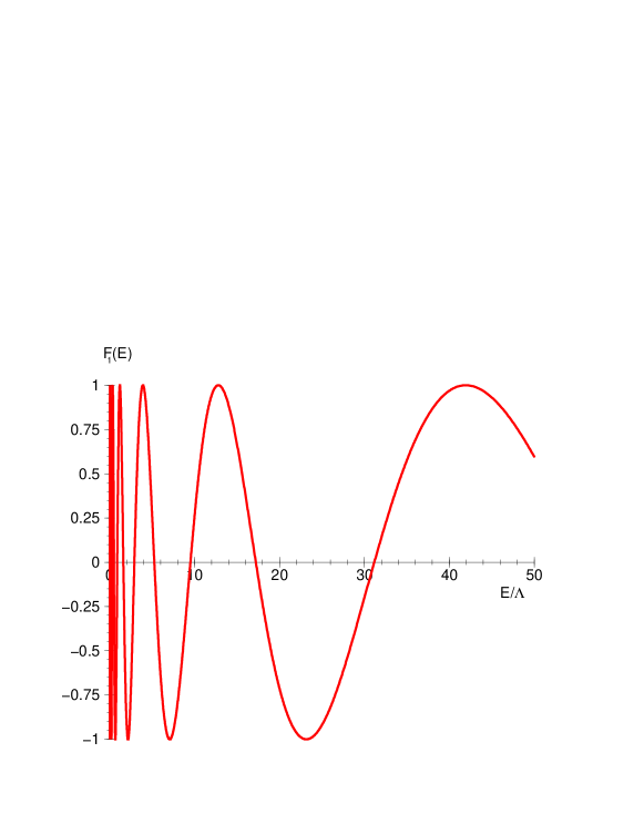
Figure 8: The function $F_{1}(E)$.

We conclude this section with a general comment. The rule concerning the position of renormalons in field theory is that we find on the positive semiaxis the renormalons corresponding to strongly coupled physics. For asymptotically free gauge theories IR renormalons are at $z>0$, while UV renormalons are at $z<0$. In QED or $\lambda\phi^{4}$ the coupling becomes strong in the UV and correspondingly the UV renormalons are at $z>0$ and IR renormalons are at $z<0$. When a singularity is at $z>0$ we must give a prescription for going around it; if we understand the physics associated to this singularity, we can give a physically motivated prescription; then we are left with a non-perturbative contribution, but no ambiguity on the resummation of the perturbative series. This is the case of instantons [30]. If however we do not understand the physics behind the singularity, we do not know what prescription to use. Different prescriptions (e.g. going around a pole from above or from below) give answers that differ by terms of order $\exp(-2k/\beta_{0}g_{\rm YM}^{2})$, so renormalons on the positive semiaxis are usually taken as a source of an uncertainty of this order in the resummation of the perturbative series.

In our case, however, the coefficients $B_{T},C$ in eq. (66) are fixed from the comparison with the numerical solution. Once we specify the IR solution, the values of $B_{T},C$, etc. follow, and the renormalon contribution, rather than an uncertainty on the perturbative series, becomes a well defined non-perturbative contribution. The fact that IR physics fixes the renormalon contributions confirms the old conjecture of ’t Hooft [30] that renormalon singularities are related to the quark confinement mechanism. It is interesting to note that instead $B_{T},C$ cannot be fixed, even in principle, from the UV side, since there they just appear as integration constants of the homogeneous equations (52).

7 $\alpha^{\prime}$ and string loop corrections

We next consider the effect of $\alpha^{\prime}$ corrections on the solutions. For the type 0 theory, these have been discussed in ref. [11], where it is found that they have the same structure as in type II theories; in particular, world-sheet supersymmetry implies the vanishing of $\sim\alpha^{\prime}({\rm Riemann})^{2}$ corrections, and the first non-vanishing correction is $\sim\alpha^{\prime 3}({\rm Riemann})^{4}$. It is well known that $\alpha^{\prime}$ corrections suffer from a certain degree of ambiguity, because not all the coefficients of the possible operators are fixed by the comparison with the string amplitudes; a related ambiguity is the fact that one can perform field redefinitions that mix different orders in $\alpha^{\prime}$, e.g. $g_{\mu\nu}\rightarrow g_{\mu\nu}+\alpha^{\prime}R_{\mu\nu}$. If one has an exactly conformal background these field redefinitions do not matter, but of course if one works at a finite order in the $\alpha^{\prime}$ expansion they make a difference.

An important observation [12] is that we can choose the $\alpha^{\prime}$ correction such that they depend only on the Weyl tensor, rather than on the Riemann tensor, and then they have a much milder behaviour when we approach $AdS_{5}$. To be quantitative, consider eq. (8), which, including the first non-vanishing $\alpha^{\prime}$ correction, has the general form [12]

$$\ddot{\phi}+\frac{1}{2}g(T)e^{\frac{\phi+\xi}{2}-5\eta}=c\,e^{\frac{-3\phi+\xi}{2}-5\eta}\,({\rm Weyl})^{4}\,,$$ (79)

where $c$ is a constant, (Weyl)⁴ denotes the appropriate contractions of four Weyl tensors $C_{MNRS}$, and again we have set $\alpha^{\prime}=1$. Writing $\ddot{\phi}=e^{2y}(\phi^{\prime\prime}+\phi^{\prime})$, where as before the dot is $d/d\rho$ and the prime is $d/dy$, with $\rho=e^{-y}$, we have

$$\phi^{\prime\prime}+\phi^{\prime}+\frac{1}{2}g(T)e^{\frac{\phi+\xi}{2}-5\eta-2y}=c\,e^{\frac{-3\phi+\xi}{2}-5\eta-2y}\,({\rm Weyl})^{4}\,.$$ (80)

We see that an ansatz of the form (16)-(19), or its improved form (42)-(45), is still a solution, but the numerical coefficients in front of the factors $\ln 2$ change. In fact, consider the ansatz $\phi=-2\ln y+a_{1}\ln 2+O(\ln y/y),\xi=-y+a_{2}\ln 2+O(1/y),\eta=-y/2+a_{3}\ln 2+O(1/y),T=-1+O(1/y)$. We have checked that on this ansatz all components of the Weyl tensor $C_{MNRS}$ are $O(1/y)$, so that [12]

$$({\rm Weyl})^{4}\sim\frac{1}{y^{4}}\,.$$ (81)

Substituting into eq. (80) we get (setting again $g(T)=T^{2}/2$)

$$-\frac{2}{y}+\frac{1}{4y}\,e^{(\frac{a_{1}+a_{2}}{2}-5a_{3})\ln 2}+O(\frac{1}{y^{2}})=\frac{\rm const.}{y}\,e^{(\frac{-3a_{1}+a_{2}}{2}-5a_{3})\ln 2}+O(\frac{1}{y^{2}})\,,$$ (82)

and similarly for the equations for $\xi,\eta,T$. Thus, the leading $y$ dependence cancels, and we can adjust the coefficients $a_{1},a_{2},a_{3}$ so that the equations are satisfied. We see that the numerical values of the coefficients $a_{1},a_{2},a_{3}$ are affected by the inclusion of the (Weyl)⁴ term. The logarithmic behaviour in the UV is not spoiled, but the numerical values of the beta function coefficients change [12].

We now want to see whether the terms related to renormalons are affected. If we use again the improved ansatz (42)-(45), where now $b$ and the coefficients of $\ln 2$ in $\xi,\eta$ are modified according to the discussion above, we see that, in the limit $by\gg 1$, where $b/(A+by)\simeq 1/y$, the net effect of the addition of the (Weyl)⁴ term is to change the numerical factors inside the square brackets on the right-hand side of eqs. (46)–(49). However, the associated homogeneous equations are still given by eq. (52), and are unaffected by the inclusion of the (Weyl)⁴ term. Therefore, the position of the renormalon singularities in the Borel plane is unaffected by these $\alpha^{\prime 3}$ corrections. It is clear that the argument goes through at all orders in $\alpha^{\prime}$ as long as the corrections can be written in terms of the Weyl tensor. As for the string loop corrections, in the UV they are small by definition, since $e^{\phi}\ll 1$. Thus, it appears that the result on the position of renormalon singularities is quite robust.

In the IR the situation is more complicated, first of all because unavoidably when $g_{\rm YM}$ becomes strong also the string loop corrections become important. This is different from the standard AdS/CFT correspondence, where the dilaton is constant and $g_{s}=e^{\phi}$ can be taken to be small everywhere.

The role of $\alpha^{\prime}$ corrections in the IR has been discussed in ref. [14], and it has been found that they depend crucially on the numerical relations between the coefficients $\xi_{1},\phi_{1},\eta_{1}$ that parametrize the IR solution (25). With the choice $\xi_{1}=\phi_{1}$ that we used in sect. 4, the corrections are indeed large in the IR, while, for instance, for $\phi_{1}=3\xi_{1},t_{1}=0$ we still have a confining solution but now the $\alpha^{\prime}$ corrections in the IR are exponentially small in $\rho$. Therefore we have repeated the numerical analysis discussed in sect. 4, for the case $\phi_{1}=3\xi_{1},\xi_{1}=1,t_{1}=0$ and, from eq. (27), $\eta_{1}=1$. We have found that the lowest order solution for the dilaton and the tachyon shows no qualitative difference, see fig. (9).

The functions $\eta,\xi$ are also qualitatively very similar to the previous case; the main difference is that, since now $\xi_{1}/2-\eta_{1}<0$, the radius of the 5-sphere $R_{(5)}^{2}=e^{\frac{\xi}{2}-\eta}$ goes to zero in the IR, see fig. (10) (using eq. (27), we see that this happens in general if $\phi_{1}^{2}>(3/2)\xi_{1}^{2}$). This suggests that the six adjoint scalars become massive, but to clarify this point we need a better understanding of string loop corrections in the IR limit.

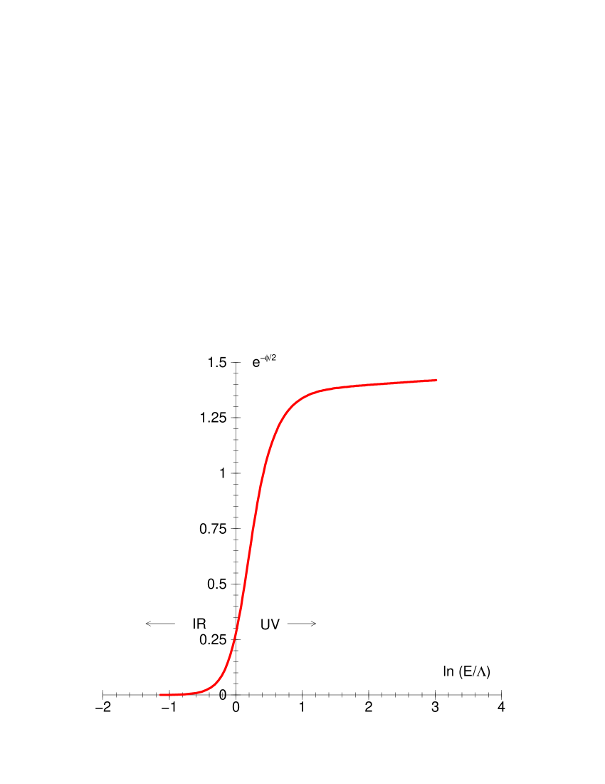
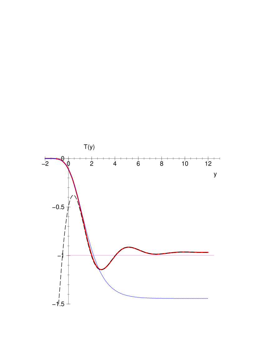
Figure 9: $e^{-\phi/2}$ and the tachyon in the case $\phi_{1}=3,\xi_{1}=1$.

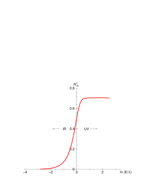
Figure 10: $R_{(5)}^{2}$ in the case $\phi_{1}=3,\xi_{1}=1$.

References

- [1] J. Maldacena, “The large N limit of superconformal field theories and supergravity,” Adv. Theor. Math. Phys. 2 (1998) 231 [hep-th/9711200].
- [2] S. S. Gubser, I. R. Klebanov and A. M. Polyakov, “Gauge theory correlators from non-critical string theory,” Phys. Lett. B428 (1998) 105 [hep-th/9802109].
- [3] E. Witten, “Anti-de Sitter space and holography,” Adv. Theor. Math. Phys. 2 (1998) 253 [hep-th/9802150].
- [4] O. Aharony, S. S. Gubser, J. Maldacena, H. Ooguri and Y. Oz, “Large N field theories, string theory and gravity,” Phys. Rept. 323 (2000) 183 [hep-th/9905111].
- [5] E. Witten, “Anti-de Sitter space, thermal phase transition, and confinement in gauge theories,” Adv. Theor. Math. Phys. 2 (1998) 505 [hep-th/9803131].
- [6] L. Girardello, M. Petrini, M. Porrati and A. Zaffaroni, “Novel local CFT and exact results on perturbations of N = 4 super Yang-Mills from AdS dynamics,” JHEP 9812 (1998) 022 [hep-th/9810126].
- [7] L. Girardello, M. Petrini, M. Porrati and A. Zaffaroni, “The supergravity dual of N = 1 super Yang-Mills theory,” Nucl. Phys. B569 (2000) 451 [hep-th/9909047].
- [8] J. Polchinski and M. J. Strassler, “The string dual of a confining four-dimensional gauge theory,” hep-th/0003136.
- [9] A. M. Polyakov, “The wall of the cave,” Int. J. Mod. Phys. A14 (1999) 645 [hep-th/9809057].
- [10] A. M. Polyakov, “String theory and quark confinement,” Nucl. Phys. Proc. Suppl. 68 (1998) 1 [hep-th/9711002].
- [11] I. R. Klebanov and A. A. Tseytlin, “D-branes and dual gauge theories in type 0 strings,” Nucl. Phys. B546 (1999) 155 [hep-th/9811035].
- [12] I. R. Klebanov and A. A. Tseytlin, “Asymptotic freedom and infrared behavior in the type 0 string approach to gauge theory,” Nucl. Phys. B547 (1999) 143 [hep-th/9812089].
- [13] J. A. Minahan, “Glueball mass spectra and other issues for supergravity duals of QCD models,” JHEP 9901 (1999) 020 [hep-th/9811156].
- [14] J. A. Minahan, “Asymptotic freedom and confinement from type 0 string theory,” JHEP 9904 (1999) 007 [hep-th/9902074].
- [15] G. Ferretti and D. Martelli, “On the construction of gauge theories from non critical type 0 strings,” Adv. Theor. Math. Phys. 3 (1999) 119 [hep-th/9811208].
- [16] G. Ferretti, J. Kalkkinen and D. Martelli, “Non-critical type 0 string theories and their field theory duals,” Nucl. Phys. B555 (1999) 135 [hep-th/9904013].
- [17] M. Alishahiha, A. Brandhuber and Y. Oz, “Branes at singularities in type 0 string theory,” JHEP 9905 (1999) 024 [hep-th/9903186].
- [18] C. Angelantonj and A. Armoni, “Non-tachyonic type 0B orientifolds, non-supersymmetric gauge theories and cosmological RG flow,” hep-th/9912257.
- [19] C. Angelantonj and A. Armoni, “RG flow, Wilson loops and the dilaton tadpole,” hep-th/0003050.
- [20] A. Armoni, E. Fuchs and J. Sonnenschein, “Confinement in 4D Yang-Mills theories from non-critical type 0 string theory,” JHEP 9906 (1999) 027 [hep-th/9903090].
- [21] L. J. Dixon and J. A. Harvey, “String Theories In Ten-Dimensions Without Space-Time Supersymmetry,” Nucl. Phys. B274 (1986) 93.
- [22] N. Seiberg and E. Witten, “Spin Structures In String Theory,” Nucl. Phys. B276 (1986) 272.
- [23] J. Polchinski, “String Theory”, vol. 2, Cambridge University Press, 1998.
- [24] O. Bergman and M. R. Gaberdiel, “A non-supersymmetric open-string theory and S-duality,” Nucl. Phys. B499 (1997) 183 [hep-th/9701137].
- [25] J. Maldacena, “Wilson loops in large N field theories,” Phys. Rev. Lett. 80 (1998) 4859 [hep-th/9803002].
- [26] S. Rey and J. Yee, “Macroscopic strings as heavy quarks in large N gauge theory and anti-de Sitter supergravity,” hep-th/9803001.
- [27] S. Rey, S. Theisen and J. Yee, “Wilson-Polyakov loop at finite temperature in large N gauge theory and anti-de Sitter supergravity,” Nucl. Phys. B527 (1998) 171 [hep-th/9803135].
- [28] A. Brandhuber, N. Itzhaki, J. Sonnenschein and S. Yankielowicz, “Wilson loops, confinement, and phase transitions in large N gauge theories from supergravity,” JHEP 9806 (1998) 001 [hep-th/9803263].
- [29] G. Parisi, “The physical basis of the asymptotic estimates in perturbation theory,” Cargese Summer Institute 1977.
- [30] G. ’t Hooft, “Can We Make Sense Out Of ’Quantum Chromodynamics’?,” Erice 1977, A. Zichichi ed., Plenum Press, NY 1978.
- [31] G. Altarelli, “Introduction to renormalons,” CERN-TH-95-309 International School of Subnuclear Physics: 33rd Course: Vacuum and Vacua: The Physics of Nothing, 2-10 Jul 1995, Erice, Italy.
- [32] M. Beneke, “Renormalons,” Phys. Rept. 317 (1999) 1 [hep-ph/9807443].
- [33] M. Beneke and V. I. Zakharov, “Improving large order perturbative expansions in quantum chromodynamics,” Phys. Rev. Lett. 69 (1992) 2472.
- [34] A. I. Vainshtein and V. I. Zakharov, “Ultraviolet renormalon calculus,” Phys. Rev. Lett. 73 (1994) 1207 [hep-ph/9404248].