The Trans-Planckian Problem of Inflationary Cosmology

Abstract

In most current models of inflation based on a weakly self-coupled scalar matter field minimally coupled to gravity, the period of inflation lasts so long that, at the beginning of the inflationary period, the physical wavelengths of comoving scales which correspond to the present large-scale structure of the Universe were smaller than the Planck length. Thus, the usual computations of the spectrum of fluctuations in these models involve extrapolating low energy physics (both in the matter and gravitational sector) into regions where this physics is not applicable. In this article we study the dependence of the usual predictions of inflation for the spectrum of cosmological fluctuations on the hidden assumptions about super-Planck scale physics. We introduce a class of modified dispersion relations to mimic possible effects of super-Planck scale physics, and find that, given an initial state determined by minimizing the energy density, for dispersions relations introduced by Unruh the spectrum is unchanged, whereas for a class of dispersion relations similar to those used by Corley and Jacobson (which involve a more radical departure from the usual linear relation) important deviations from the usual predictions of inflation can be obtained. Some implications of this result for the unification of fundamental physics and early Universe cosmology are discussed.

PACS numbers: 98.80.Cq, 98.70.Vc

]

I Introduction

The inflationary Universe scenario [1] is the first theory of the very early Universe to provide a mechanism [2] for the production of density fluctuations on scales of cosmological interest based on causal physics (see also Ref. [3] for initial ideas). The key point is that during the period of inflation fixed comoving scales are stretched exponentially compared to the Hubble radius. Thus, the wavelengths corresponding to the present large-scale structure in the Universe and to the measured Cosmic Microwave Background (CMB) anisotropies were equal to the Hubble radius about 50 Hubble expansion times before the end of inflation. This gives rise to the possibility that causal physics acting before that time can generate fluctuations on these scales while they are of sub-Hubble length.

Most current models of inflation are based on weakly self-coupled scalar matter fields minimally coupled to gravity. In this context, quantum vacuum fluctuations provide [2] a causal mechanism for generating fluctuations. In fact, the coupled linear metric and matter fluctuations can be quantized in a unified manner [4]. The problem reduces to the quantization of a free scalar field with a time-dependent mass (see e.g. Ref. [5] for a comprehensive review). An initial vacuum state thus undergoes squeezing during inflation, and this leads to the generation of fluctuations. According to the standard calculations [2, 6, 7, 8, 9, 10], the predicted spectrum is scale-invariant (modulo a mild deviation from scale-invariance which stems from the time-dependence of the Hubble constant during the inflationary period).

There are good heuristic reasons [3] to expect a scale-invariant spectrum of fluctuations to emerge from inflation. Since de-Sitter space is time-translation-invariant, one should expect the amplitude of the density fluctuations ${\delta M}/M$ to be independent of the scale (labelled by the comoving wavenumber $n$) if measured at the time when the corresponding wavelength crosses the Hubble radius $l_{\rm H}$ during the inflationary period. Since microphysics cannot change the physical amplitude of the mass fluctuations while the wavelength is larger than $l_{\rm H}$, one therefore expects ${\delta M}/M$ to be independent of $n$ when measured at the time $t_{\rm f}(n)$ when the scale re-enters the Hubble radius in the post-inflationary Friedmann-Robertson-Walker period:

$${{\delta M}\over M}\bigl{(}n,t_{\rm f}(n)\bigr{)}\,=\,{\rm const.}\,,$$ (1)

which is the definition of a scale-invariant Harrison-Zel’dovich spectrum [11].

The time-translation-invariance is, however, broken in the current models of inflation. The calculations are done by picking an initial time $t_{\rm i}$ (e.g. the beginning of the inflationary period), by choosing a specific state of the quantum fields at this time (e.g. the local Minkowski vacuum state [10] or the Bunch-Davies vacuum [12]), by evolving this state using the linearized equations of motion, and by finally calculating the correlation functions and expectation values of interest. In this context, the emergence of a scale-invariant spectrum of fluctuations is seen to arise from a subtle cancellation of the wavenumber dependence in the initial state wave function and in the growth factor before Hubble radius crossing, and thus depends explicitly on the initial state chosen. States can be found [13] which do not yield a scale-invariant spectrum. Thus, it is clear that the prediction of a Harrison-Zel’dovich spectrum is not completely generic in current models of inflation.

There is, however, a much more serious potential problem for the claim that current models of inflation based on weakly self-coupled scalar fields generically lead to a scale-invariant spectrum of fluctuations. Most of these models of inflation involve (see e.g. [14] for a recent review) a period of inflation much longer than the 60 e-foldings of inflation required to solve the horizon and flatness problems of standard cosmology. Since wavelengths exponentially redshift during inflation, the physical wavelengths of the modes which correspond to the present large-scale structure in the Universe were, in those models, much smaller than the Planck length at the initial time $t_{\rm i}$. Thus, the usual computations of the spectrum of fluctuations involve extrapolating weakly self-coupled field theory coupled to classical gravity into a regime where these theories are known to break down.

This problem is analogous to the Trans-Planckian problem for black hole physics (see Ref. [15] for a recent overview). In black hole physics there is an arbitrarily large blue shift when following modes of Hawking radiation at future infinity into the past, and the usual calculations of Hawking radiation [16] seem suspect (see e.g. Ref. [17] for a discussion of this point).

In the case of the black hole problem, it was recently shown by Unruh [18], Brout et al. [19], Hambli and Burgess [20] and by Corley and Jacobson [21] that the prediction of a thermal Hawking spectrum of black hole radiation is insensitive to modifications of the physics at the ultraviolet end of the spectrum. In these works, the dispersion relation of the quantum fields was modified (in rather ad-hoc ways) at energies larger than some ultraviolet scale $k_{\rm C}$, and it was found that the spectrum of radiation at future infinity at wavenumbers much smaller than $k_{\rm C}$ is insensitive to the modifications considered. In this sense, Hawking radiation from black holes was shown to be an infrared effect.

The obvious question is whether a similar conclusion will hold for the generation of fluctuations in inflationary cosmology. This is the question we will address in this paper. We will consider a free scalar field in an inflationary background [de Sitter phase of a Friedmann-Robertson-Walker cosmology with scale factor $a(t)$]. This scalar field can represent the scalar metric fluctuations, the gravitational wave mode, or a matter scalar field on the fixed background geometry - the case of most interest for cosmology corresponds to scalar metric fluctuations. We will modify the usual dispersion relation

$$\omega^{2}=k^{2},\quad k^{2}\equiv{{n^{2}}\over{a^{2}}},$$ (2)

where $n$ and $k$ are the comoving and physical wavenumbers, respectively, for values of $k$ larger than some cutoff scale $k_{\rm C}$, and will calculate the predicted spectrum of fluctuations in the modified theory for well-motivated initial quantum states, states which in the unmodified theory coincide with the state usually chosen as the initial state. The modified dispersion relations which we use are the same as the ones used by Unruh [18] and by Corley and Jacobson [21]. As preferred initial states we will use either the state which minimizes the energy density at the initial time $t_{\rm i}$, following the approach of Brown and Dutton [23], or a naive generalization of the local Minkowski vacuum.

We find that in the case of Unruh’s dispersion relation, the spectrum of density fluctuations is unchanged in the minimum energy density initial state. However, in the case of the family of dispersion relations generalizing the choice of Corley and Jacobson, the choice of the minimum energy density initial state leads to a spectrum of fluctuations which, depending on the specific member of the family of dispersion relations chosen, may be characterized by a tilt, by an exponential factor, and by superimposed oscillations.

Our work indicates that the prediction of a scale-invariant spectrum in inflationary cosmology depends sensitively on hidden assumptions about super-Planck-scale physics. This has important implications for the attempts to unify fundamental physics and early Universe cosmology. It is now a rather nontrivial question under which conditions a unified theory of all forces such as string or M-theory will lead to a scale-invariant spectrum, assuming for the moment that it does indeed lead to a period of inflation.

The outline of this paper is as follows. In Section II we demonstrate that the growth of linear density fluctuations, gravitational waves and linear scalar matter fluctuations can all be described in terms of the same framework: that of a free scalar field with a time-dependent mass. In Section III we introduce the two classes of modified dispersion relations which will be used in the calculations. The quantization of the scalar field in the time-dependent background and the construction of the minimum energy density initial state are reviewed in Section IV. Section V contains our calculations for both classes of dispersion relations. Our results are summarized and discussed in the final section.

II Equivalence between cosmological perturbations and a fictitious scalar field

Without loss of generality, the line element for the spatially flat Friedmann-Lemaître-Robertson-Walker (FLRW) background plus the perturbations can be written in the synchronous gauge according to [24, 25]:

$${\rm d}s^{2} = a^{2}(\eta)\biggl{\{}-{\rm d}\eta^{2}+\biggl{[}\delta_{ij}+h(\eta,{\bf n})Q\delta_{ij}$$ (4)

$$+h_{l}(\eta,{\bf n})\frac{Q_{,i,j}}{n^{2}}+h_{\rm gw}(\eta,{\bf n})Q_{ij}\biggr{]}{\rm d}x^{i}{\rm d}x^{j}\biggr{\}}.$$

In this equation, the dimensionless quantity ${\bf n}$ is the comoving wavevector related to the physical wavevector ${\bf k}$ through the relation ${\bf k}\equiv{\bf n}/a(\eta)$. $\eta$ is the conformal time related to the cosmic time $t$ by ${\rm d}t=a(\eta){\rm d}\eta$. The functions $h$ and $h_{l}$ represent the scalar sector and $Q(x^{i})$ is the eigenfunction of the Laplace operator on the flat spacelike hypersurfaces. The function $h_{\rm gw}$ represents the gravitational waves and $Q_{ij}(x^{i})$ is the eigentensor of the Laplace operator. It is traceless and transverse, namely $Q_{i}{}^{i}=Q_{ij}{}^{,j}=0$. It is convenient to introduce the background quantity $\gamma(\eta)$ defined by $\gamma\equiv-\dot{H}/H^{2}$, where a dot means differentiation with respect to cosmic time and $H$ is the Hubble rate, $H\equiv\dot{a}/a$. We can also write $\gamma=1-{\cal H}^{\prime}/{\cal H}^{2}$, where ${\cal H}\equiv a^{\prime}/a$ and a prime denotes differentiation with respect to the conformal time.

In the tensor sector, we define the quantity $\mu_{\rm T}$ by $h_{\rm gw}\equiv\mu_{\rm T}/a$. Then, the equation of motion is given by [26]:

$$\mu_{{\rm T}}^{\prime\prime}+\biggl{[}n^{2}-\frac{a^{\prime\prime}}{a}\biggr{]}\mu_{{\rm T}}=0.$$ (5)

Since gravitational waves do not couple to matter, the last equation is valid for every type of matter.

In the scalar sector, it is convenient to work with a residual gauge invariant variable $\mu_{\rm S}$ defined by $\mu_{\rm S}\equiv[a/({\cal H}\sqrt{\gamma})](h^{\prime}+{\cal H}\gamma h)$ where we have supposed $\gamma\neq 0$. The case $\gamma=0$ must be treated separately (see below). The quantity $\mu_{\rm S}$ is related to the gauge invariant Bardeen potential by $\Phi_{\rm B}^{({\rm SG})}=[{\cal H}\gamma/(2n^{2})][\mu_{\rm S}/(a\sqrt{\gamma})]^{\prime}$ where the subscript ‘${\rm SG}$’ means ‘calculated in the synchronous gauge’ [27]. Therefore, knowing the solution for $\mu_{\rm S}$ permits the calculation of the Bardeen variable. If matter is described by a scalar field (the inflaton), then one can show that $\mu_{\rm S}$ obeys the equation:

$$\mu_{{\rm S}}^{\prime\prime}+\biggl{[}n^{2}-\frac{(a\sqrt{\gamma})^{\prime\prime}}{(a\sqrt{\gamma})}\biggr{]}\mu_{{\rm S}}=0.$$ (6)

The case $\gamma=0$ corresponds to a scale factor $a(t)\propto e^{Ht}$, i.e. to the de Sitter manifold. Then, one can show that the exact solution to the perturbed Einstein equations is $\Phi_{\rm B}=0$: there are no density perturbations at all. This is because when the equation of state is $p=-\rho$, fluctuations of the inflaton are not coupled to fluctuations of the perturbed metric. Coupling occurs only as a result of the violation of the condition $p=-\rho$.

Observable quantities can be computed when the initial power spectra are known. These are defined in terms of the two-point correlation functions. For the Bardeen potential one has

$$\langle 0|\Phi_{\rm B}(\eta,{\bf x}) \Phi_{\rm B}(\eta,{\bf x}+{\bf r})|0\rangle$$ (8)

$$\equiv\int_{0}^{+\infty}\frac{{\rm d}n}{n}\frac{\sin nr}{nr}n^{3}P_{\rm\Phi_{\rm B}}(\eta,n),$$

whereas for gravitational waves the correlator is given by

$$\langle 0|h_{ij}(\eta,{\bf x})h^{ij}(\eta,{\bf x}+{\bf r})|0\rangle\equiv\int_{0}^{+\infty}\frac{{\rm d}n}{n}\frac{\sin nr}{nr}n^{3}P_{\rm h}(\eta,n),$$ (9)

where we have written $h_{ij}=h_{\rm gw}Q_{ij}$. We are specially interested in modes which are outside the horizon at the end of inflation, i.e. $n/(aH)\ll 1$. For these modes, the power spectra do not depend on time and can be written as

$$n^{3}P_{\rm\Phi_{\rm B}}(n)=A_{\rm S}n^{n_{\rm S}-1},\quad n^{3}P_{\rm h}(n)=A_{\rm T}n^{n_{\rm T}}.$$ (10)

Let us now consider power law inflation models where the scale factor is given by $a(\eta)=l_{0}|\eta|^{1+\beta}$ where $\beta$ is a number such that $\beta\leq-2$ and $l_{0}$ has the dimension of a length. The advantage of this class of models is that everything can be calculated exactly. In the case $\beta=-2$ which corresponds to exponential expansion, the length $l_{0}$ is nothing but the Hubble radius, $l_{\rm H}\equiv a^{2}/a^{\prime}$ . The function $\gamma$ is a constant given by $\gamma=(\beta+2)/(\beta+1)$ which vanishes for $\beta=-2$. We see that Eq. (6) now reduces to Eq. (5). The spectral indices can be determined exactly and read

$$n_{\rm S}=2\beta+5,\quad n_{\rm T}=2\beta+4.$$ (11)

We have the relation $n_{\rm S}-1=n_{\rm T}$ which is valid exactly only for power law inflation.

Let us now consider a massless scalar field $\Phi(\eta,{\bf x})$ living in a FLRW spacetime. It is convenient to Fourier decompose the field and to introduce the quantity $\mu$ defined according to $\Phi(\eta,{\bf x})\equiv[1/(2\pi)^{3/2}]\int{\rm d}{\bf n}(\mu/a)e^{i{\bf n}\cdot{\bf x}}$. It is easy to show that the Klein-Gordon equation reduces to the following equation for $\mu$

$$\mu^{\prime\prime}+\biggl{[}n^{2}-\frac{a^{\prime\prime}}{a}\biggr{]}\mu=0.$$ (12)

This equation is exactly the same as Eq. (5) and Eq. (6). Therefore, investigating the properties of cosmological perturbations is equivalent to investigating the properties of a fictitious scalar field $\Phi(\eta,{\bf x})$. In particular, the calculation of the power spectrum of the scalar and tensor perturbations reduces to the computation of the power spectrum of this fictitious scalar field. In the following, we will restrict our considerations to this case, having in mind that, in fact, we will calculate the power spectra of cosmological perturbations.

Let us make a last remark. Although it seems that we have considered only a limited class of models (i.e. power law inflation), the previous analogy is in fact much more general. This is because the slow roll approximation, valid for a wide class of inflationary models, reduces to first order to power law inflation.

III Time dependent dispersion relations

In this section, we present the two classes of modified dispersion relations that will be used in this article. Let us return to the equation of motion (12). In this equation, the presence of the term $n^{2}$ is due to the differential operator $\delta^{ij}{\rm\partial}_{i}{\rm\partial}_{j}$ in the Klein-Gordon equation. In Fourier space, this means that

$$\omega^{2}=k^{2}=\frac{n^{2}}{a^{2}}.$$ (13)

The dispersion relation is therefore linear in the physical wavenumber $k$: $\omega=k$. A possible alteration of the high frequency behaviour of the Klein-Gordon equation can be obtained if we require the presence of a nonlinear function $F(k)$ such that $\omega=F(k)$ which, for physical wavenumbers smaller than a new characteristic scale $k_{\rm C}$, i.e. $k\ll k_{\rm C}$, reduces to $\omega\approx k$. This means that the $n^{2}$ term in the Klein-Gordon equation should now be replaced with a time dependent $n_{\rm eff}^{2}(\eta)$ such that

$$n_{\rm eff}^{2}=a^{2}(\eta)F^{2}(k)=a^{2}(\eta)F^{2}[n/a(\eta)].$$ (14)

We see that, in terms of comoving wavenumbers, we obtain a time dependent dispersion relation. In what follows, we will consider two explicit examples for the function $n_{\rm eff}$. Given the modified dispersion relation, Eq. (12) can now be written as

$$\mu^{\prime\prime}+\biggl{[}n_{\rm eff}^{2}-\frac{a^{\prime\prime}}{a}\biggr{]}\mu=0.$$ (15)

Let us analyze this equation in more detail. We can distinguish three regimes. In Region I, the wavelength of a given mode, $\lambda(\eta)\equiv(2\pi/n)a(\eta)$, is much smaller than the characteristic length: $\lambda\ll l_{\rm C}$. The nonlinearities in the dispersion relation play an important role and the solution of the equation of motion depends on the particular form of $F(k)$. A crucial issue is that the mode no longer behaves as a free wave initially. As a consequence, the choice of initial conditions cannot be done in the usual way. In Region II, the wavelength of the mode is larger than the characteristic length but still smaller than the Hubble radius, $l_{\rm C}\ll\lambda\ll l_{\rm H}$. In this case, one can consider the dispersion relation to be linear, i.e. $\Omega(\eta)\approx 0$ and neglect the term $a^{\prime\prime}/a$. Therefore, the solution can be expressed as:

$$\mu_{\rm II}(\eta)\,=\,B_{1}e^{in\eta}+B_{2}e^{-in\eta}\,.$$ (16)

Finally, in Region III, the mode is outside the Hubble radius: $\lambda\gg l_{\rm H}$ and the solution (the growing mode) is given by:

$$\mu_{\rm III}(\eta)\,=\,Ca(\eta)\,,$$ (17)

where $C$ is a $n$ dependent constant. This constant has to be determined by performing the matching of $\mu$ and $\mu^{\prime}$ at the times of transition between regions I and II and regions II and III, $\eta_{1}$ and $\eta_{2}$ respectively. Then, the spectrum can be calculated and reads

$$n^{3}P_{\rm\Phi}=n^{3}\biggl{|}\frac{\mu}{a}\biggr{|}^{2}=n^{3}|C|^{2}.$$ (18)

Let us now turn to the first example of a time dependent modified dispersion relation.

A Unruh’s dispersion relation

The dispersion relation used by Unruh in Ref. [18], in the context of black holes physics, is:

$$\omega=F(k)\equiv k_{\rm C}\tanh^{1/p}\biggl{[}\biggl{(}\frac{k}{k_{\rm C}}\biggr{)}^{p}\biggl{]},$$ (19)

where $p$ is an arbitrary coefficient. For large values of the wave number, this becomes a constant $k_{\rm C}$ whereas for small values this is a linear law as expected. According to Eq. (14), in the context of cosmology, we take

$$n_{\rm eff}(\eta)=\frac{2\pi a(\eta)}{l_{\rm C}}\tanh^{1/p}\biggl{[}\biggl{(}\frac{nl_{\rm C}}{2\pi a(\eta)}\biggr{)}^{p}\biggl{]},$$ (20)

where $l_{\rm C}$ is the characteristic length corresponding to $k_{\rm C}$. The argument of the hyperbolic tangent can also be rewritten as $l_{\rm C}/\lambda(\eta)$. This means that when $\lambda\gg l_{\rm C}$, $n_{\rm eff}(\eta)$ tends to $n$.

B Generalized Corley/Jacobson dispersion relation

The dispersion relation utilized by Corley and Jacobson in Ref. [21] is given by the following expression

$$\omega^{2}=F^{2}(k)\equiv k^{2}-\frac{k^{4}}{k_{\rm C}^{2}}.$$ (21)

In this article, we consider a more general case and write

$$\omega^{2}=k^{2}+k^{2}\sum_{q=1}^{m}b_{q}\biggl{(}\frac{k}{k_{\rm C}}\biggr{)}^{2q},$$ (22)

where the $b_{q}$ are, a priori, arbitrary coefficients. Let us suppose that the previous sum only contains the last term. The physics depends on the sign of $b_{m}$. If $b_{m}$ is negative, then $\omega$ vanishes for $k=k_{\rm C}|b_{m}|^{-2m}$. Beyond this point, the dispersion relation becomes complex. The Corley/Jacobson case corresponds to $m=1$ and $b_{1}=-1$. In the context of cosmology, the previous ansatz gives rise to the following function $n_{\rm eff}(\eta)$

$$n_{\rm eff}^{2}(\eta)=n^{2}+n^{2}\sum_{q=1}^{m}\frac{b_{q}}{(2\pi)^{2q}}\biggl{(}\frac{l_{\rm C}}{a}\biggr{)}^{2q}n^{2q}.$$ (23)

Again, when $\lambda\gg l_{\rm C}$ then the effective comoving wavenumber simply reduces to $n$. On the other hand, when $\lambda\ll l_{\rm C}$, one has

$$n_{\rm eff}^{2}\,\approx\,\frac{b_{m}}{(2\pi)^{2m}}\biggl{(}\frac{l_{\rm C}}{a}\biggr{)}^{2m}n^{2m+2}\,.$$ (24)

The different dispersion relations used in this article are displayed in Fig. (1) together with the dispersion relation considered in Ref. [22] denoted “KG”.

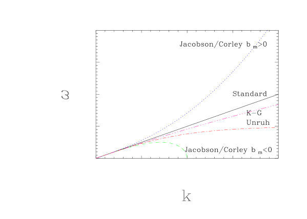
FIG. 1.: Sketch of the different dispersion relations.

IV Quantization of a massive scalar field

The aim of this section is to develop a Lagrangian and Hamiltonian formalism for the system described above. We will show that considering a time-dependent dispersion relation is equivalent to giving a time-dependent mass to the fictitious scalar field. The main purpose of this section is to discuss the initial conditions. As already mentioned previously, when the wavelength of a mode is smaller than the critical length $l_{\rm C}$, the mode does not behave as a free wave because the dispersion relation in this region is no longer $\omega=k$. As a consequence, it is no longer possible to impose the usual initial condition at $\eta=\eta_{\rm i}$, i.e. $\mu\rightarrow e^{-in(\eta-\eta_{\rm i})}/\sqrt{2n}$. Another method must be used. Following Ref. [23], we will choose the state which initially minimizes the energy density of the field.

A Lagrangian and Hamiltonian formalisms

We now study a massive fictitious scalar field $\Phi$ whose action is given by

$$S = \int{\rm d}\eta\int_{R^{3+}}{\rm d}{\bf n}\biggl{[}\mu_{\bf n}^{\prime}\mu_{\bf n}^{*^{\prime}}+\frac{a^{{}^{\prime}2}}{a^{2}}\mu_{\bf n}\mu_{\bf n}^{*}$$ (26)

$$-\frac{a^{\prime}}{a}(\mu_{\bf n}^{\prime}\mu_{\bf n}^{*}+\mu_{\bf n}\mu_{\bf n}^{*^{\prime}})-n_{\rm eff}^{2}\mu_{\bf n}\mu_{\bf n}^{*}\biggr{]}.$$

In this equation, the scalar field has been Fourier expanded according to

$$\Phi(\eta,{\bf x})=\frac{1}{(2\pi)^{3/2}}\frac{1}{a(\eta)}\int{\rm d}{\bf n}\mu_{\bf n}(\eta)e^{i{\bf n}\cdot{\bf x}},$$ (27)

and $\mu_{\bf n}(\eta)$ denotes the complex Fourier component of the field. We can easily check that the Lagrange equation of motion for the quantity $\mu_{\bf n}(\eta)$ leads to Eq. (15).

We are now in a position where we can pass to the Hamiltonian formalism. Our first move is to perform the following time-dependent transformation

$$\mu_{\bf n}(\eta)\equiv\frac{1}{N(n,\eta)}\psi_{\bf n}(\eta),$$ (28)

where $N(n,\eta)$ is a time-dependent factor which will be fixed below. Next, the action given in Eq. (26) expressed in terms of the new variable $\psi_{\bf n}(\eta)$ takes the form

$$S = \int{\rm d}\eta\int_{R^{3+}}{\rm d}{\bf n}\biggl{[}\frac{1}{N^{2}}\psi_{\bf n}^{\prime}\psi_{\bf n}^{*^{\prime}}+\frac{1}{N^{2}}\biggl{(}\frac{N^{\prime}}{N}+\frac{a^{\prime}}{a}\biggr{)}^{2}\psi_{\bf n}\psi_{\bf n}^{*}$$ (31)

$$-\frac{1}{N^{2}}\biggl{(}\frac{N^{\prime}}{N}+\frac{a^{\prime}}{a}\biggr{)}\biggl{(}\psi_{\bf n}^{\prime}\psi_{\bf n}^{*}+\psi_{\bf n}\psi_{\bf n}^{*^{\prime}}\biggr{)}$$

$$-\frac{1}{N^{2}}n_{\rm eff}^{2}\psi_{\bf n}\psi_{\bf n}^{*}\biggr{]}.$$

We can now calculate the conjugate momentum to $\psi_{\bf n}(\eta)$. Its definition is $p_{\bf n}\equiv{\rm\partial}\bar{{\cal L}}_{\bf n}/{\rm\partial}\psi_{\bf n}^{*}(\eta)$ where $\bar{{\cal L}}_{\bf n}$ is the Lagrangian density (the bar indicates that one calculates the Lagrangian in Fourier space) which one can deduce from the previous equation. The conjugate momentum reads

$$p_{\bf n}=\frac{1}{N^{2}}\biggl{(}\psi_{\bf n}^{\prime}-\frac{a^{\prime}}{a}\psi_{\bf n}\biggr{)}-\frac{N^{\prime}}{N^{3}}\psi_{\bf n}.$$ (32)

The Hamiltonian can be determined using the following relation

$$\bar{{\cal H}}_{\bf n}\equiv p_{\bf n}\psi_{\bf n}^{*^{\prime}}+p_{\bf n}^{*}\psi_{\bf n}^{\prime}-\bar{{\cal L}}_{\bf n}.$$ (33)

Inserting the expressions of the Lagrangian and of the the conjugate momentum in this definition, we obtain

$$\bar{{\cal H}}_{\bf n} = N^{2}p_{\bf n}p_{\bf n}^{*}+\frac{(aN)^{\prime}}{aN}\biggl{(}\psi_{\bf n}p_{\bf n}^{*}+\psi_{\bf n}^{*}p_{\bf n}\biggr{)}$$ (35)

$$+\frac{1}{N^{2}}n_{\rm eff}^{2}\psi_{\bf n}\psi_{\bf n}^{*}.$$

The explicit quantization can now be carried out. We express the Fourier component $\psi_{\bf n}$ and its conjugate momentum $p_{\bf n}$ in terms of creation and annihilation operators, satisfying the usual commutation relation $[c_{\bf n},c_{\bf r}^{\dagger}]=\delta({\bf n}-{\bf r})$, according to

$$\psi_{\bf n}\equiv\sqrt{\hbar}\biggl{(}c_{\bf n}+c_{-{\bf n}}^{\dagger}\biggr{)},\quad p_{\bf n}\equiv\frac{\sqrt{\hbar}}{2i}\biggl{(}c_{\bf n}-c_{-{\bf n}}^{\dagger}\biggr{)}.$$ (36)

The Hamiltonian operator is obtained by plugging the previous expressions into Eq. (35) and requiring that ‘$\hbar\omega/2$’ be present in each mode, which fixes the normalization factor $N$ to be

$$N^{2}\,=\,2\omega(\eta)\,,$$ (37)

where $\omega$ is the ‘comoving frequency’ defined by $\omega(\eta)\equiv n_{\rm eff}$. Although we use the same notation for convenience, this frequency should not be confused with the physical frequency which appears in Eqns. (19) and (21) and which can obtained by multiplying the comoving frequency by a factor $1/a$. The Hamiltonian reads

$$H= \int_{R^{3}}{\rm d}{\bf n}\biggl{[}\frac{\hbar\omega}{2}\biggl{(}c_{\bf n}c_{\bf n}^{\dagger}+c_{-{\bf n}}c_{-{\bf n}}^{\dagger}\biggr{)}+\frac{i\hbar}{2}\frac{(a\sqrt{\omega})^{\prime}}{a\sqrt{\omega}}\biggl{(}c_{-{\bf n}}^{\dagger}c_{\bf n}^{\dagger}$$ (39)

$$-c_{-{\bf n}}c_{\bf n}\biggr{)}\biggr{]}.$$

This Hamiltonian has the usual structure. The first term is just a collection of harmonic oscillators whereas the second term represents the interaction between the background and the perturbations. This term is responsible for the phenomenon of particle creation, which is a squeezing effect. In a static spacetime, the pump function $(a\sqrt{\omega})^{\prime}/(a\sqrt{\omega})$ vanishes and the interaction part of the Hamiltonian disappears. The field operator can be expressed as

$$\Phi(\eta,{\bf x}) = \frac{\sqrt{\hbar}}{a(\eta)}\frac{1}{(2\pi)^{3/2}}\int\frac{{\rm d}{\bf n}}{\sqrt{2\omega(\eta)}}\biggl{[}c_{\bf n}(\eta)e^{i{\bf n}\cdot{\bf x}}$$ (41)

$$+c_{\bf n}^{\dagger}(\eta)e^{-i{\bf n}\cdot{\bf x}}\biggr{]}.$$

The time evolution of the creation and annihilation operators and therefore of the quantum scalar field is calculated by means of the Heisenberg equation:

$$i\hbar\frac{{\rm d}}{{\rm d}\eta}c_{\bf n}(\eta)=[c_{\bf n},H].$$ (42)

Using the form of the Hamiltonian derived previously, one gets the following equations of motion

$$i\hbar\frac{{\rm d}c_{\bf n}}{{\rm d}\eta} = \hbar\omega(\eta)c_{\bf n}+i\hbar\frac{(a\sqrt{\omega})^{\prime}}{a\sqrt{\omega}}c_{-{\bf n}}^{\dagger},$$ (43)

$$i\hbar\frac{{\rm d}c_{\bf n}^{\dagger}}{{\rm d}\eta} = -\hbar\omega(\eta)c_{\bf n}^{\dagger}+i\hbar\frac{(a\sqrt{\omega})^{\prime}}{a\sqrt{\omega}}c_{-{\bf n}}.$$ (44)

The solution of these equations is a Bogoliubov transformation which can be written as

$$c_{\bf n}(\eta) = u_{n}(\eta)c_{\bf n}(\eta_{\rm i})+v_{n}(\eta)c_{-{\bf n}}^{\dagger}(\eta_{\rm i}),$$ (45)

$$c_{\bf n}^{\dagger}(\eta) = u_{n}^{*}(\eta)c_{\bf n}^{\dagger}(\eta_{\rm i})+v_{n}^{*}(\eta)c_{-{\bf n}}(\eta_{\rm i}),$$ (46)

where we have introduced two new functions $u_{n}(\eta)$ and $v_{n}(\eta)$. These functions satisfy $|u_{n}(\eta)|^{2}-|v_{n}(\eta)|^{2}=1$ in order for the commutation relation given to be preserved in time. Let us notice that $u_{n}$ and $v_{n}$ do not depend on the vector ${\bf n}$ but only on its modulus $n$. Inserting the previous equations in Eqns. (43) and (44), one obtains the equation of motion for these two functions

$$i\hbar\frac{{\rm d}u_{n}}{{\rm d}\eta} = \hbar\omega(\eta)u_{n}+i\hbar\frac{(a\sqrt{\omega})^{\prime}}{a\sqrt{\omega}}v_{n}^{*},$$ (47)

$$i\hbar\frac{{\rm d}v_{n}}{{\rm d}\eta} = \hbar\omega(\eta)v_{n}+i\hbar\frac{(a\sqrt{\omega})^{\prime}}{a\sqrt{\omega}}u_{n}^{*}.$$ (48)

The functions $u_{n}$ and $v_{n}$ can be re-expressed in terms of three other arbitrary functions $r_{n}(\eta)$, $\theta_{n}(\eta)$ and $\varphi_{n}(\eta)$. Following this path would lead to the squeezed state formalism. However, we will not need it in this article.

B Fixing the initial conditions

The previous considerations permit to fix the initial value of the mode function $\mu_{n}(\eta_{\rm i})$ and its derivative $\mu_{n}^{\prime}(\eta_{\rm i})$ for any choice of function $\Omega(\eta)$, i.e. for any time dependent dispersion relation.

It is straightforward to check that the function

$$\mu_{n}\equiv\frac{1}{N(n,\eta)}(u_{n}+v_{n}^{*})=\frac{1}{\sqrt{2\omega}}(u_{n}+v_{n}^{*}),$$ (49)

satisfies Eq. (15). From Eqns. (45) and (46), we see that the initial conditions for the two function $u_{n}$ and $v_{n}$ are given by: $u_{n}(\eta=\eta_{\rm i})=1$ and $v_{n}(\eta=\eta_{\rm i})=0$. Therefore, the initial value of the mode function $\mu$ can be written as:

$$\mu(\eta=\eta_{\rm i})=\frac{1}{\sqrt{2\omega(\eta_{\rm i})}}=\frac{1}{\sqrt{2n_{\rm eff}}}.$$ (50)

Let us now turn to the determination of $\mu^{\prime}(\eta=\eta_{\rm i})$. It will be found by the requirement that the energy density is minimized. The stress energy tensor can be obtained from the action (26) with the help of the standard definition. In terms of the Fourier components $\psi_{n}$, the energy density reads

$$\rho = \frac{\hbar}{4\pi^{2}a^{4}}\int_{0}^{\infty}\frac{{\rm d}n}{N^{2}}\biggl{[}\psi_{n}^{\prime}\psi_{n}^{*^{\prime}}-\frac{(aN)^{\prime}}{aN}(\psi_{n}\psi_{n}^{*^{\prime}}+\psi_{n}^{\prime}\psi_{n}^{*})$$ (53)

$$+\frac{a^{\prime 2}}{a^{2}}\psi_{n}\psi_{n}^{*}+\frac{N^{\prime 2}}{N^{2}}\psi_{n}\psi_{n}^{*}+n_{\rm eff}^{2}\psi_{n}\psi_{n}^{*}$$

$$+2\frac{a^{\prime}N^{\prime}}{aN}\psi_{n}\psi_{n}^{*}\biggr{]}.$$

We now define the functions $x(\eta)$ and $y(\eta)$ as the real and imaginary parts of the ratio $\psi_{n}^{\prime}/\psi_{n}\equiv x+iy$, respectively. Then, the initial energy density can be expressed in terms of $x_{\rm i}\equiv x(\eta=\eta_{\rm i})$, $y_{\rm i}\equiv y(\eta=\eta_{\rm i})$ and the Wronskian $W(n)\equiv\mu_{n}^{\prime}\mu_{n}^{*}-\mu_{n}^{*^{\prime}}\mu_{n}$ which is a time independent quantity (as can be checked in calculating ${\rm d}W(n)/{\rm d}\eta$ and using the equation of motion for $\mu_{n}$)

$$\rho = \frac{\hbar}{4\pi^{2}a^{4}}\int_{0}^{\infty}{\rm d}n\frac{W(n)}{2iy_{\rm i}}\biggl{[}x_{\rm i}^{2}+y_{\rm i}^{2}-2\frac{(aN)^{\prime}}{aN}x_{\rm i}+\frac{a^{\prime 2}}{a^{2}}$$ (54)

$$+ n_{\rm eff}^{2}+\frac{N^{\prime 2}}{N^{2}}+2\frac{a^{\prime}N^{\prime}}{aN}\biggr{]},$$ (55)

where $N$ and $a$ are also evaluated at the initial time. Notice that, while deriving the previous equation, we used the fact that the Wronskians of $\mu_{n}$ and $\psi_{n}$ are related by a factor $N^{2}$. The ‘vacuum’ used in this article is defined as the state which initially minimizes the energy density. The variation of the previous expression with respect to $x_{\rm i}$ and $y_{\rm i}$ leads to

$$\delta\rho = \frac{\hbar}{4\pi^{2}a^{4}}\int_{0}^{\infty}{\rm d}n\frac{W(n)}{2i}\biggl{\{}\frac{2}{y_{\rm i}}\biggl{[}x_{\rm i}-\frac{(aN)^{\prime}}{aN}\biggr{]}\delta x_{\rm i}$$ (58)

$$+\frac{1}{y_{\rm i}^{2}}\biggl{[}y_{\rm i}^{2}-x_{\rm i}^{2}+2\frac{(aN)^{\prime}}{aN}x_{\rm i}-\frac{a^{\prime 2}}{a^{2}}-n_{\rm eff}^{2}$$

$$-\frac{N^{\prime 2}}{N^{2}}-2\frac{a^{\prime}N^{\prime}}{aN}\biggl{]}\delta y_{\rm i}\biggr{\}}.$$

Demanding that $\delta\rho=0$, one deduces the initial values of $x$ and $y$

$$x_{\rm i}=\frac{a^{\prime}}{a}(\eta_{\rm i})+\frac{N^{\prime}}{N}(\eta_{\rm i}),\quad y_{\rm i}=\pm n_{\rm eff}.$$ (59)

These expressions can be simplified. Using the explicit form of the function $N(n,\eta)$, one can write

$$\frac{N^{\prime}}{N}=\frac{\omega^{\prime}}{2\omega}.$$ (60)

At the time $\eta=\eta_{\rm i}$, it is reasonable to consider $\lambda\ll l_{\rm C}$ (otherwise, the whole problem studied here would be pointless). Then, for Unruh’s dispersion relation, one finds $N^{\prime}/N\approx a^{\prime}/2a$ and for the Corley/Jacobson dispersion relation, one has $N^{\prime}/N\approx-ma^{\prime}/2a$. In addition, $a^{\prime}/a$ is very small in the limit where the conformal time goes to $-\infty$ since $a^{\prime}/a(\eta_{\rm i})=(1+\beta)/|\eta_{\rm i}|$ and $|\eta_{\rm i}|\gg 1$. Therefore, one gets that $\psi_{n}^{\prime}/\psi_{n}\approx iy_{\rm i}$. On the other hand, we have $\mu_{n}=\psi_{n}/N$. Combining this formula with the previous one, one obtains $\mu_{n}^{\prime}+N^{\prime}/N=iy_{\rm i}\mu_{n}$. Neglecting again the term $N^{\prime}/N$, we finally arrive at

$$\mu^{\prime}(\eta=\eta_{\rm i})=\pm i\sqrt{\frac{n_{\rm eff}}{2}}.$$ (61)

The initial conditions are now completely fixed and given by Eqns. (50) and (61).

Let us also mention that it is possible to adopt another choice of initial conditions which corresponds to the ‘instantaneous Minkowski vacuum’ at $\eta=\eta_{\rm i}$, namely

$$\mu(\eta_{\rm i})=\frac{1}{\sqrt{2n}},\quad\mu^{\prime}(\eta_{\rm i})=\pm i\sqrt{\frac{n}{2}}.$$ (62)

If the dispersion relation is standard, then $\Omega=0$ and the mode is initially free: locally, it does not feel the curvature of space-time and behaves as it were flat. In this case, the two possible choices of initial conditions discussed above coincide.

Two last comments are in order before ending this section. Let us first remark that the concept of an initial state which minimizes the energy density of the field could be problematic in a region where the dispersion relation becomes complex, as it is the case for the Corley/Jacobson dispersion relation with $b_{m}<0$, since the energy needs not to be bounded from below in such a situation. We are not aware of any more obvious method than the one used here to deal with this case.

Finally, although we have introduced two initial states, it should be clear that the minimizing energy state is the only physical vacuum state. The instantaneous Minkowski vacuum is considered here only to stress the fact that the choice of the initial conditions becomes more crucial than in the standard situation where one can show that a large class of initial states leads to the same spectrum [28] (although, as already mentioned in the introduction, it is possible to find examples which do not belong to this class of initial states [13]).

V Analytical solutions

In this section, we calculate the spectrum of fluctuations for the two classes of dispersion relations introduced in Section III. We focus on a fixed comoving wavenumber $n$ and proceed as follows. We solve the equation of motion in each of the three regions (defined in Section III) separately. The coefficients of the two fundamental solutions in Region I are fixed by the initial conditions discussed above. Then, we explicitly perform the matching of $\mu$ and $\mu^{\prime}$ at the transitions between Region I and Region II, which occurs at a time denoted by $\eta_{1}$, and between Region II and Region III, which occurs at time $\eta_{2}$, to obtain the coefficients of the two fundamental solutions in Region III, from which the spectrum can be calculated. The time $\eta_{2}$ is when the mode crosses the Hubble radius, which is given by

$$l_{\rm H}(\eta)\,=\,\frac{l_{0}}{|1+\beta|}|\eta|^{2+\beta}\,.$$ (63)

Thus, the condition $l_{\rm H}(\eta_{2})=\lambda(\eta_{2})$ boils down to

$$|\eta_{2}|=\frac{2\pi}{n}|1+\beta|\,.$$ (64)

The geometry of space-time is illustrated in Fig. (2).

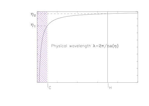
FIG. 2.: Sketch of the evolution of a physical mode throughout the three regions defined in the text. The dashed region is the region where the dispersion relation is modified.

We start this section with Unruh’s dispersion relation.

A Unruh’s case

The equation of motion for the mode function can be written as

$$\mu^{\prime\prime}+\biggl{\{}\frac{4\pi^{2}}{l_{\rm C}^{2}}a^{2}\tanh^{2/p}\biggl{[}\biggl{(}\frac{l_{\rm C}}{\lambda(\eta)}\biggr{)}^{p}\biggl{]}-\frac{a^{\prime\prime}}{a}\biggr{\}}\mu=0.$$ (65)

This equation can be solved exactly in Region I only if the scale factor is given by $a(\eta)=l_{0}/|\eta|$, i.e. in the case $\beta=-2$. Fortunately, this corresponds to the de Sitter space-time, the prototypical model of inflationary cosmology. Note that in this case $l_{0}$ is the Hubble radius [see Eq. (63)]. In Region I, the hyperbolic tangent is approximatively one since $l_{\rm C}\gg\lambda$ initially. Therefore, Equation (65) reduces to

$$\mu^{\prime\prime}+\biggl{(}\frac{4\pi^{2}l_{0}^{2}/l_{\rm C}^{2}-2}{\eta^{2}}\biggr{)}\mu=0.$$ (66)

Note that, in fact, the form of this last equation is independent of the precise form (i.e. the hyperbolic tangent) of the dispersion relation in the regime $l_{\rm C}\gg\lambda$. It is just necessary to assume that $F(k)$ goes to a constant. We see that the result depends in an essential way on the dimensionless parameter $\epsilon\equiv l_{\rm C}/l_{0}$. At this point, we have assumed nothing about the value of the ratio $l_{\rm C}/l_{0}$. However, physically, it is clear that $\epsilon\ll 1$. One would expect the cutoff length to be given by the Planck length ($l_{\rm C}\approx l_{\rm Pl}$), whereas $l_{0}\approx 10^{5}l_{\rm Pl}$ if the spectrum of fluctuations is COBE normalized. In this case, we have $\epsilon\approx 10^{-5}$. In the following, we will use an expansion in terms of this parameter. The exact solution of Eq. (66) is

$$\mu_{\rm I}(\eta)=A_{1}|\eta|^{x_{1}}+A_{2}|\eta|^{x_{2}},$$ (67)

where the exponents $x_{1}$ and $x_{2}$ are given by

$$x_{1,2}=\frac{1}{2}\pm\frac{1}{2}\sqrt{9-\frac{16\pi^{2}}{\epsilon^{2}}}.$$ (68)

It is now time to fix the coefficients $A_{1}$ and $A_{2}$. They are completely determined by the initial conditions (50) and (61). In the approximation where $l_{\rm C}\gg\lambda$, they are solutions of (note that we do not yet use the fact that $\epsilon$ is small)

$$A_{1}|\eta_{\rm i}|^{x_{1}}+A_{2}|\eta_{\rm i}|^{x_{2}} = \frac{1}{2}\sqrt{\frac{\epsilon}{\pi}}|\eta_{\rm i}|^{1/2},$$ (69)

$$A_{1}x_{1}|\eta_{\rm i}|^{x_{1}-1}+A_{2}x_{2}|\eta_{\rm i}|^{x_{2}-1} = \mp i\sqrt{\frac{\pi}{\epsilon}}|\eta_{\rm i}|^{-1/2}.$$ (70)

The exact solution of this system of equations can be written as

$$A_{1} = |\eta_{\rm i}|^{1/2-x_{1}}\frac{1}{1-x_{1}/x_{2}}\frac{1}{2}\sqrt{\frac{\epsilon}{\pi}}\biggl{(}1\pm\frac{2i\pi}{\epsilon x_{2}}\biggr{)},$$ (71)

$$A_{2} = |\eta_{\rm i}|^{1/2-x_{2}}\frac{1}{1-x_{2}/x_{1}}\frac{1}{2}\sqrt{\frac{\epsilon}{\pi}}\biggl{(}1\pm\frac{2i\pi}{\epsilon x_{1}}\biggr{)}.$$ (72)

It is at this point that we use the fact that $\epsilon$ is small. To first order in a systematic expansion in this parameter we obtain

$$A_{1} \approx \frac{i}{8}\biggl{(}\frac{\epsilon}{\pi}\biggr{)}^{3/2}\biggl{(}\frac{1}{2}-\frac{2i\pi}{\epsilon}\pm\frac{2i\pi}{\epsilon}\biggr{)}$$ (74)

$$\times\exp\biggl{(}-\frac{2i\pi}{\epsilon}\ln\bigl{|}\eta_{\rm i}\bigr{|}\biggr{)},$$

$$A_{2} \approx \frac{i}{8}\biggl{(}\frac{\epsilon}{\pi}\biggr{)}^{3/2}\biggl{(}\frac{1}{2}+\frac{2i\pi}{\epsilon}\pm\frac{2i\pi}{\epsilon}\biggr{)}$$ (76)

$$\times\exp\biggl{(}\frac{2i\pi}{\epsilon}\ln\bigl{|}\eta_{\rm i}\bigr{|}\biggr{)}.$$

We now pursue the calculation for both choices of the sign of the initial conditions. We introduce an index ‘u’ for the upper choice and ‘l’ for the lower choice. This leads to

$$A_{1}^{u} = \frac{i}{16}\biggl{(}\frac{\epsilon}{\pi}\biggr{)}^{3/2}\exp\biggl{(}-\frac{2i\pi}{\epsilon}\ln\bigl{|}\eta_{\rm i}\bigr{|}\biggr{)},$$ (77)

$$A_{2}^{u} = \frac{1}{2}\biggl{(}\frac{\epsilon}{\pi}\biggr{)}^{1/2}\exp\biggl{(}\frac{2i\pi}{\epsilon}\ln\bigl{|}\eta_{\rm i}\bigr{|}\biggr{)},$$ (78)

$$A_{1}^{l} = \frac{1}{2}\biggl{(}\frac{\epsilon}{\pi}\biggr{)}^{1/2}\exp\biggl{(}-\frac{2i\pi}{\epsilon}\ln\bigl{|}\eta_{\rm i}\bigr{|}\biggr{)},$$ (79)

$$A_{2}^{l} = -\frac{i}{16}\biggl{(}\frac{\epsilon}{\pi}\biggr{)}^{3/2}\exp\biggl{(}\frac{2i\pi}{\epsilon}\ln\bigl{|}\eta_{\rm i}\bigr{|}\biggr{)}.$$ (80)

Therefore, one has $A_{2}^{u}\gg A_{1}^{u}$, $A_{1}^{l}\gg A_{2}^{l}$ and only one branch of the solution (67) survives. Then, the solution in Region I can be expressed as

$$\mu_{\rm I}^{u,l}(\eta)=\frac{1}{2}\sqrt{\frac{\epsilon|\eta|}{\pi}}\exp\biggl{(}\mp\frac{2i\pi}{\epsilon}\ln\biggl{|}\frac{\eta}{\eta_{\rm i}}\biggr{|}\biggr{)}.$$ (81)

Let us now turn to Region II. As already mentioned above, in this region, the solution is given by

$$\mu_{\rm II}(\eta)\,=\,B_{1}e^{in\eta}+B_{2}e^{-in\eta}\,.$$ (82)

The coefficients $B_{1}$ and $B_{2}$ are determined by the matching of this solution with the solution (81) at the time $\eta_{1}$. Continuity of $\mu$ and $\mu^{\prime}$ yields

$$inB_{1}e^{in\eta_{1}} + inB_{2}e^{-in\eta_{1}}$$ (83)

$$= \frac{in}{2}\biggl{(}\frac{\epsilon|\eta_{1}|}{\pi}\biggr{)}^{1/2}\exp\biggl{(}\mp\frac{2i\pi}{\epsilon}\ln\biggl{|}\frac{\eta_{1}}{\eta_{\rm i}}\biggr{|}\biggr{)},$$ (84)

$$inB_{1}e^{in\eta_{1}} - inB_{2}e^{-in\eta_{1}}$$ (85)

$$= \pm i\biggl{(}\frac{\pi}{\epsilon|\eta_{1}|}\biggr{)}^{1/2}\exp\biggl{(}\mp\frac{2i\pi}{\epsilon}\ln\biggl{|}\frac{\eta_{1}}{\eta_{\rm i}}\biggr{|}\biggr{)}.$$ (86)

The solution can be found easily and reads

$$B_{1} = \frac{1}{2\sqrt{n}}(1\pm 1)\exp\biggl{(}\mp\frac{2i\pi}{\epsilon}\ln\biggl{|}\frac{\eta_{1}}{\eta_{\rm i}}\biggr{|}+\frac{2i\pi}{\epsilon}\biggr{)},$$ (87)

$$B_{2} = \frac{1}{2\sqrt{n}}(1\mp 1)\exp\biggl{(}\mp\frac{2i\pi}{\epsilon}\ln\biggl{|}\frac{\eta_{1}}{\eta_{\rm i}}\biggr{|}-\frac{2i\pi}{\epsilon}\biggr{)},$$ (88)

As a consequence, the solution in Region II also contains only one branch.

Finally, we must solve the mode equation in Region III. As already mentioned, the non-decaying mode is

$$\mu_{\rm III}=Ca(\eta)\,.$$ (89)

The coefficient $C$ is fixed by the matching of the mode function when the mode crosses the horizon at $\eta_{2}$ . One gets

$$C\,=\,\mu_{\rm II}(\eta_{2})\frac{|\eta_{2}|}{l_{0}}=\frac{2\pi}{n}\frac{\mu_{\rm II}(\eta_{2})}{l_{0}}\,.$$ (90)

Therefore, regardless of the choice of the sign of the initial conditions, we have $|C|\propto 1/n^{3/2}$ and as a result

$$n^{3}P_{\rm\Phi}\propto n^{0}\,.$$ (91)

We see that, when $\beta=-2$, the final answer is not changed compared to what is obtained without the modification of the dispersion relation, i.e. we get a scale invariant spectrum $n_{\rm S}=1$ [see Eq. (11)].

We now discuss different initial conditions. We adopt the ‘instantaneaous Minkowski’ initial conditions given by Eqns. (62). Of course, the form of the solution in Region I is still the same but, now, the coefficients $A_{1}$ and $A_{2}$ are different. The exact expressions for theses coefficients can now be written as

$$A_{1} = \pm\sqrt{\frac{n}{2}}\frac{i}{x_{2}-x_{1}}|\eta_{\rm i}|^{1-x_{1}}\biggl{(}1\mp\frac{ix_{2}}{n|\eta_{\rm i}|}\biggr{)},$$ (92)

$$A_{2} = \pm\sqrt{\frac{n}{2}}\frac{i}{x_{1}-x_{2}}|\eta_{\rm i}|^{1-x_{2}}\biggl{(}1\mp\frac{ix_{1}}{n|\eta_{\rm i}|}\biggr{)}.$$ (93)

In the limit when the parameter $\epsilon$ is small, an expansion of the previous expressions leads to the following formulas

$$A_{1}\approx\frac{1}{2\sqrt{2n}}|\eta_{\rm i}|^{-2i\pi/\epsilon-1/2},\quad A_{2}\approx\frac{1}{2\sqrt{2n}}|\eta_{\rm i}|^{2i\pi/\epsilon-1/2}.$$ (94)

The result does not depend on the choice of the sign of the initial conditions. We see also another crucial difference in comparison with the previous case, see Eq. (74) and (76): this time, the coefficients are of the same order in $\epsilon$. Therefore, the solution in Region I is now given by a cosine instead of by a pure phase

$$\mu_{\rm I}(\eta)=\frac{1}{\sqrt{2n}}\biggl{|}\frac{\eta}{\eta_{\rm i}}\biggr{|}^{1/2}\cos\biggl{(}\frac{2\pi}{\epsilon}\ln\biggl{|}\frac{\eta}{\eta_{\rm i}}\biggr{|}\biggr{)}.$$ (95)

The solution in Region II is still given by plane waves. The matching at time $\eta_{1}$ permits the calculation of the coefficients $B_{1}$ and $B_{2}$. They read

$$B_{1} = \frac{1}{2n}\sqrt{\frac{\pi}{\epsilon|\eta_{\rm i}|}}\exp\biggl{(}-in\eta_{1}-\frac{2\pi i}{\epsilon}\ln\biggl{|}\frac{\eta_{1}}{\eta_{\rm i}}\biggr{|}\biggr{)},$$ (96)

$$B_{2} = \frac{1}{2n}\sqrt{\frac{\pi}{\epsilon|\eta_{\rm i}|}}\exp\biggl{(}in\eta_{1}+\frac{2\pi i}{\epsilon}\ln\biggl{|}\frac{\eta_{1}}{\eta_{\rm i}}\biggr{|}\biggr{)}.$$ (97)

Again, there is an important difference in comparison with the previous case: both coefficients are now non vanishing. The mode function in Region II can be expressed as

$$\mu_{\rm II}(\eta)=\frac{1}{n}\sqrt{\frac{\pi}{\epsilon|\eta_{\rm i}|}}\cos\biggl{(}n\eta-n\eta_{1}+\frac{2\pi}{\epsilon}\ln\biggl{|}\frac{\eta_{1}}{\eta_{\rm i}}\biggr{|}\biggr{)}.$$ (98)

The function is proportional to $1/n$ instead of $1/\sqrt{n}$. The determination of the constant $C$ proceeds as previously and leads to the spectrum

$$n^{3}P_{\rm\Phi}\propto n^{-1}\cos^{2}\biggl{(}\frac{2\pi}{\epsilon}+\frac{2\pi}{\epsilon}\ln\biggl{|}\frac{2\pi}{n\eta_{\rm i}}\biggr{|}\biggr{)}.$$ (99)

A few remarks are in order here. Firstly, the difference between (91) and (99) demonstrates that the final result does depend on the choice of the initial conditions. Secondly, the spectral index is now modified and is $n_{\rm S}=0$ instead of $n_{\rm S}=1$ previously. Thirdly, oscillations in the spectrum are present. If $n_{1}$ and $n_{2}$ are two wave numbers such that the argument of the cosine differs by a factor $2\pi p$ where $p$ is an integer then one has $n_{2}/n_{1}=\exp(p\epsilon)$. This means that unless $p$ is comparable to $\epsilon^{-1}$, $n_{1}$ and $n_{2}$ are almost equal. Therefore, the oscillations are very rapid.

B The Corley/Jacobson case

With the dispersion relation (22), the equation of motion becomes

$$\mu^{\prime\prime}+\mu\biggl{[}n^{2}+n^{2}\sum_{q=1}^{m}\frac{b_{q}}{(2\pi)^{2q}}\biggl{(}\frac{\epsilon\,n}{|\eta|^{1+\beta}}\biggr{)}^{2q}-\frac{a^{\prime\prime}}{a}\biggr{]}=0.$$ (100)

This equation is valid for any scale factor of the form $a(\eta)=l_{0}|\eta|^{1+\beta}$. Unlike in Unruh’s case, we do not need to specify $\beta=-2$.

We now need to discuss the form of the solution in Region I. This crucially depends on the sign of the coefficient $b_{m}$. In the regime we are interested in, i.e. $l_{\rm C}\gg\lambda(\eta_{\rm i})$, one can retain only the dominate term and the dispersion relation can be written as

$$n_{\rm eff}^{2}\approx n^{2}+n^{2}b_{m}\biggl{(}\frac{l_{\rm C}}{\lambda}\biggr{)}^{2m}.$$ (101)

This means that if $b_{m}$ is positive, the dispersion relation remains real. If $b_{m}$ is negative the situation is more complicated. For very small value of $|b_{m}|$, the dispersion relation can remain real even in the regime $l_{\rm C}\gg\lambda(\eta_{\rm i})$. However, it seems a bit artificial to fine-tune the value of $|b_{m}|$ such that this actually happens. Without this fine-tuning the dispersion relation certainly becomes complex. This last property should not be considered as a surprise. Indeed there exist many situations in Physics where complex dispersion relations appear. This is for example the case in Hydrodynamics when one describes the damping of a sound wave in a fluid due to viscosity [29]. Then, the dispersion relation is given by $k=\omega/c+ia\omega^{2}$ where $a$ is a factor which depends on the viscosity coefficients. In Cosmology, other examples are Silk damping or damping of density perturbations due to neutrino decoupling [30]. In this paper, we choose to analyze both cases and write $b_{m}\equiv s|b_{m}|$ with $s=\pm 1$. Then, from Eqns. (50) and (61), the quantities $\mu_{\rm I}(\eta_{\rm i})$ and $\mu_{\rm I}^{\prime}(\eta_{\rm i})$ take the form

$$\mu_{\rm I}(\eta_{\rm i}) = \frac{s^{-1/4}}{\sqrt{2b\gamma}}|\eta_{i}|^{1/2-b/2},$$ (102)

$$\mu_{\rm I}^{\prime}(\eta_{\rm i}) = \pm is^{1/4}\sqrt{\frac{b\gamma}{2}}|\eta_{i}|^{-1/2+b/2},$$ (103)

where we have defined $b$ and $\gamma$ (not to be confused with the function $\gamma$ used in Section II) by the following expressions

$$b\equiv 1-m(1+\beta),\quad\gamma\equiv\frac{\sqrt{|b_{m}|}}{b(2\pi)^{m}}\epsilon^{m}n^{m+1}.$$ (104)

From the expressions (102) and (103), we deduce

$$\mu^{\prime}_{\rm I}(\eta_{\rm i})/\mu_{\rm I}(\eta_{\rm i})\,=\,\pm is^{1/2}b\gamma|\eta_{i}|^{b-1}\,.$$ (105)

This ratio will out turn to be important in the calculation of the various coefficients determined by the matching procedure. To go further, we need to treat the cases $s=\pm 1$ separately.

1 The case $s=-1$, $b_{m}<0$

In Region I, the equation of motion for the mode function reduces to

$$\mu^{\prime\prime}+n^{2}\frac{b_{m}}{(2\pi)^{2m}}\biggl{(}\frac{\epsilon\,n}{|\eta|^{1+\beta}}\biggr{)}^{2m}\mu=0.$$ (106)

For a negative coefficient $b_{m}$, the exact solution of Eq. (106) can be expressed in terms of modified Bessel functions as follows

$$\mu_{\rm I}(\eta)=A_{1}|\eta|^{1/2}I_{\nu}(z)+A_{2}|\eta|^{1/2}K_{\nu}(z),$$ (107)

where $\nu\equiv 1/(2b)$ and where the function $z(\eta)$ is defined by the following expression $z(\eta)\equiv\gamma|\eta|^{b}$. The coefficients $A_{1}$ and $A_{2}$ are determined by the initial conditions given in Eqns. (102) and (103). These coefficients should satisfy the system of equations

$$A_{1}I_{\nu}(z_{\rm i})+A_{2}K_{\nu}(z_{\rm i}) = |\eta_{\rm i}|^{-1/2}\mu_{\rm I}(\eta_{\rm i}),$$ (108)

$$-A_{1}I_{\nu-1}(z_{i})+A_{2}K_{\nu-1}(z_{i}) = \frac{|\eta_{\rm i}|^{1/2-b}}{\gamma b}\mu_{\rm I}^{\prime}(\eta_{\rm i}),$$ (109)

where $z_{\rm i}$ denotes the value of $z(\eta)$ at time $\eta=\eta_{\rm i}$. The exact solution for $A_{1}$ and $A_{2}$ can be expressed as

$$A_{1} = \gamma|\eta_{\rm i}|^{b-1/2}\mu_{\rm I}(\eta_{\rm i})K_{\nu-1}(z_{\rm i})$$ (111)

$$\times\biggl{[}1-\frac{|\eta_{\rm i}|^{1-b}}{\gamma b}\frac{\mu_{\rm I}^{\prime}(\eta_{\rm i})}{\mu_{\rm I}(\eta_{\rm i})}\frac{K_{\nu}(z_{\rm i})}{K_{\nu-1}(z_{\rm i})}\biggr{]},$$

$$A_{2} = \gamma|\eta_{\rm i}|^{b-1/2}\mu_{\rm I}(\eta_{\rm i})I_{\nu-1}(z_{\rm i})$$ (113)

$$\times\biggl{[}1+\frac{|\eta_{\rm i}|^{1-b}}{\gamma b}\frac{\mu_{\rm I}^{\prime}(\eta_{\rm i})}{\mu_{\rm I}(\eta_{\rm i})}\frac{I_{\nu}(z_{\rm i})}{I_{\nu-1}(z_{\rm i})}\biggr{]}.$$

In the derivation of the previous expressions, we used the exact equation: $(I_{\nu}K_{\nu-1}+I_{\nu-1}K_{\nu})(z)=1/z$. Since, when $l_{\rm C}\gg\lambda(\eta_{i})$, the argument $z_{\rm i}$ is large we can now rewrite these equations using the asymptotic formulas for Bessel functions of large arguments [31]. Notice that it is necessary to go to the second order in the expansion of the modified Bessel functions. We obtain

$$A_{1} \approx \biggl{(}\frac{\pi}{2}\biggr{)}^{1/2}\gamma^{1/2}\mu_{\rm I}(\eta_{\rm i})|\eta_{\rm i}|^{b/2-1/2}e^{-z_{\rm i}}$$ (115)

$$\times\biggl{[}1\pm 1\pm\frac{2\nu-1}{2\gamma}|\eta_{\rm i}|^{-b}\biggr{]},$$

$$A_{2} \approx \biggl{(}\frac{1}{2\pi}\biggr{)}^{1/2}\gamma^{1/2}\mu_{\rm I}(\eta_{\rm i})|\eta_{\rm i}|^{b/2-1/2}e^{z_{\rm i}}$$ (117)

$$\times\biggl{[}1\mp 1\mp\frac{1-2\nu}{2\gamma}|\eta_{\rm i}|^{-b}\biggr{]}.$$

For the sake of completeness, we pursue the calculation for both choices of the sign of the initial conditions. Let us again use an index “u” for the upper choice and “l” for the lower choice. We obtain:

$$A_{1}^{u} = 2\biggl{(}\frac{\pi}{2}\biggr{)}^{1/2}\gamma^{1/2}\mu_{\rm I}(\eta_{\rm i})|\eta_{\rm i}|^{b/2-1/2}e^{-z_{\rm i}},$$ (118)

$$A_{2}^{u} = \biggl{(}\frac{1}{2\pi}\biggr{)}^{1/2}\mu_{\rm I}(\eta_{\rm i})|\eta_{\rm i}|^{-b/2-1/2}\frac{2\nu-1}{2\gamma^{1/2}}e^{z_{\rm i}},$$ (119)

$$A_{1}^{l} = \biggl{(}\frac{\pi}{2}\biggr{)}^{1/2}\mu_{\rm I}(\eta_{\rm i})|\eta_{\rm i}|^{-b/2-1/2}\frac{1-2\nu}{2\gamma^{1/2}}e^{-z_{\rm i}},$$ (120)

$$A_{2}^{l} = 2\biggl{(}\frac{1}{2\pi}\biggr{)}^{1/2}\gamma^{1/2}\mu_{\rm I}(\eta_{\rm i})|\eta_{\rm i}|^{b/2-1/2}e^{z_{\rm i}}.$$ (121)

The exponential factor always determines the behaviour of the coefficients for any power of $|\eta_{\rm i}|$. This implies $A_{1}^{u}\approx A_{1}^{l}\approx 0$. We also see the following crucial effect: it turns out that for one choice of the sign of the derivative the first term in the squared bracket in Eqns. (115) and (117) cancels whereas for the other choice it is no longer the case. This has as a consequence that the dependence on $\gamma$ is not the same. Since $\gamma$ depends on $n$, the $n$ dependence of $A_{2}^{u}$ and $A_{2}^{l}$ is not the same. We have $A_{2}^{u}\propto\gamma^{-1}A_{2}^{l}$.

The second step of the calculation is to perform the matching of the solutions at the time $\eta=\eta_{1}$. This will allow us to express the coefficients $B_{1}$ and $B_{2}$ in terms of the coefficients $A_{1}$ and $A_{2}$. In Region II, the solution is given by plane waves. Therefore, the coefficients $B_{1}$ and $B_{2}$ are now solutions of the equations

$$B_{1}e^{in\eta_{1}}+B_{2}e^{-in\eta_{1}} = A_{1}|\eta_{1}|^{1/2}I_{\nu}(z_{1})$$ (123)

$$+A_{2}|\eta_{1}|^{1/2}K_{\nu}(z_{1}),$$

$$B_{1}e^{in\eta_{1}}-B_{2}e^{-in\eta_{1}} = -\frac{\gamma b}{in}A_{1}|\eta_{1}|^{b-1/2}I_{\nu-1}(z_{1})$$ (125)

$$+\frac{\gamma b}{in}A_{2}|\eta_{1}|^{b-1/2}K_{\nu-1}(z_{1}),$$

where $z_{1}$ is the value of the function $z(\eta)$ at $\eta=\eta_{1}$. The exact solution of this system of equations can be easily found and reads

$$e^{in\eta_{1}}B_{1} = \frac{A_{1}}{2}|\eta_{1}|^{1/2}I_{\nu}(z_{1})\biggl{[}1+\frac{i\gamma b}{n}|\eta_{1}|^{b-1}\frac{I_{\nu-1}(z_{1})}{I_{\nu}(z_{1})}\biggr{]}$$ (127)

$$+\frac{A_{2}}{2}|\eta_{1}|^{1/2}K_{\nu}(z_{1})\biggl{[}1-\frac{i\gamma b}{n}|\eta_{1}|^{b-1}\frac{K_{\nu-1}(z_{1})}{K_{\nu}(z_{1})}\biggr{]},$$

$$e^{-in\eta_{1}}B_{2} = \frac{A_{1}}{2}|\eta_{1}|^{1/2}I_{\nu}(z_{1})\biggl{[}1-\frac{i\gamma b}{n}|\eta_{1}|^{b-1}\frac{I_{\nu-1}(z_{1})}{I_{\nu}(z_{1})}\biggr{]}$$ (129)

$$+\frac{A_{2}}{2}|\eta_{1}|^{1/2}K_{\nu}(z_{1})\biggl{[}1+\frac{i\gamma b}{n}|\eta_{1}|^{b-1}\frac{K_{\nu-1}(z_{1})}{K_{\nu}(z_{1})}\biggr{]}.$$

Much simpler (approximate) formulas can be obtained if one notices that the argument of the Bessel function is a big number $z_{1}=\gamma|\eta_{1}|^{b}\gg 1$, essentially because $\epsilon$ is a small number in realistic cases. A very simple estimate allows us to quickly check the validity of this approximation. We take $m=1$, $|b_{1}|=1$, $\beta=-2.2$ which would correspond to a spectral index of $n_{\rm S}=0.6$ for power law inflation and $\epsilon=10^{-5}$ as already discussed in the previous section. We can then estimate $z_{1}$ for $n=4\pi$ which corresponds to the mode which re-enters horizon today and which consequently mainly determines the value of the CMB quadrupole anisotropy. We find $z_{1}\approx 4.7\times 10^{4}$. Therefore, we can again use the asymptotic behaviour of the Bessel function to simplify the previous equations. Putting all these ingredients together, we find

$$B_{1} \approx \frac{A_{2}}{2}\biggl{(}\frac{\pi}{2\gamma}\biggr{)}^{1/2}|\eta_{1}|^{1/2-b/2}e^{-in\eta_{1}-z_{1}-i\frac{\pi}{4}},$$ (130)

$$B_{2} \approx \frac{A_{2}}{2}\biggl{(}\frac{\pi}{2\gamma}\biggr{)}^{1/2}|\eta_{1}|^{1/2-b/2}e^{in\eta_{1}-z_{1}+i\frac{\pi}{4}}.$$ (131)

As a consequence, the solution in Region II can be written as

$$\mu_{\rm II}(\eta)=A_{2}\biggl{(}\frac{\pi}{2\gamma}\biggr{)}^{1/2}|\eta_{1}|^{1/2-b/2}e^{-z_{1}}\cos\biggl{(}n\eta-n\eta_{1}-\frac{\pi}{4}\biggr{)}.$$ (132)

The last step of the calculation is to perform the matching at $\eta=\eta_{2}$ when the mode leaves the Hubble radius (boundary between Region II and Region III). As already mentioned, in Region III, the non-decaying solution is the super-Hubble function given by

$$\mu_{\rm III}(\eta)=Ca(\eta)\,.$$ (133)

Repeating the same procedure as for Unruh’s case, the spectra can easily be calculated and read

$$n^{3}P_{\rm\Phi}^{l} \propto n^{2\beta+4}e^{2(z_{\rm i}-z_{1})}\cos^{2}\biggl{(}n\eta_{2}-n\eta_{1}-\frac{\pi}{4}\biggr{)},$$ (134)

$$n^{3}P_{\rm\Phi}^{u} \propto n^{2\beta+2-2m}e^{2(z_{\rm i}-z_{1})}\cos^{2}\biggl{(}n\eta_{2}-n\eta_{1}-\frac{\pi}{4}\biggr{)}.$$ (135)

We see that the spectrum depends explicitly on the initial conditions chosen. We can check that the tilt is correct by noticing that $n^{3}P_{\rm\Phi}\propto A_{2}^{2}$, $\gamma\propto n^{m+1}$ and using the relation between $A_{2}^{u}$ and $A_{2}^{l}$ already mentioned. From now on, we concentrate on the lower case which corresponds to an unmodified tilt and study the expression of the corresponding spectrum in more details (for convenience, we drop the subscript ‘l’). First, as mentioned above, we see that the power-law part is not modified in comparison with the usual case, i.e. the spectral index is still $n_{\rm S}=2\beta+5$. Secondly, there are oscillations in the spectrum since the argument of the cosine can be written as (considering for simplicity that $|b_{m}|=1$)

$$2\pi|1+\beta|-\biggl{(}\frac{\epsilon}{2\pi}\biggr{)}^{1/(1+\beta)}n^{(2+\beta)/(1+\beta)}-\frac{\pi}{4}.$$ (136)

However, contrary to Unruh’s case with Minkowski initial conditions, no logarithmic dependence is present. Interestingly enough, for $\beta=-2$, the oscillations disappear. The most important part concerns the exponential factor. The factor $z_{\rm i}-z_{1}$ is equal to $z_{\rm i}-z_{1}=\gamma|\eta_{\rm i}|^{b}(1-|\eta_{1}|^{b}/|\eta_{\rm i}^{b})\approx\gamma|\eta_{\rm i}|^{b}=z_{\rm i}$ since we have $|\eta_{\rm i}|\gg|\eta_{1}|$. The factor $z_{\rm i}$ can be re-written in such a way that the dependence on $n$ is explicit

$$z_{\rm i}=\frac{\sqrt{|b_{m}|}}{b(2\pi)^{m}}\epsilon^{m}|\eta_{\rm i}|^{1-m(1+\beta)}n^{m+1}.$$ (137)

The important factor in this expression is $\epsilon^{m}|\eta_{\rm i}|^{1-m(1+\beta)}$ since the others ones are of order one. It can be re-written as

$$\epsilon^{m}|\eta_{\rm i}|^{1-m(1+\beta)}=\biggl{[}\frac{l_{\rm C}}{a(\eta_{\rm i})}\biggr{]}^{m}|\eta_{\rm i}|,$$ (138)

and must be considered as large since $|\eta_{\rm i}|\gg 1$ and $l_{\rm C}/a(\eta_{\rm i})\approx l_{\rm C}/\lambda(\eta_{\rm i})\gg 1$, at least for wavenumbers not too different from $2\pi$. This means that the influence of the exponential factor is dominant and is responsible for a huge increase of the spectrum at large $n$. This is illustrated if we write the spectrum for $\beta=-2$ and $m=1$

$$n^{3}P_{\rm\Phi}\propto e^{An^{2}},$$ (139)

where $A\gg 1$. Such a spectrum is almost certainly in contradiction with observations.

We end this subsection with the calculation of the spectrum in the case where the initial state is the minimum energy density state. We restart from the exact expressions for the coefficients $A_{1}$ and $A_{2}$, see Eqns. (111) and (113). Using Eqns. (62), we have

$$\frac{|\eta_{\rm i}|^{1-b}}{\gamma b}\frac{\mu_{\rm I}^{\prime}(\eta_{\rm i})}{\mu_{\rm I}(\eta_{\rm i})}=\pm\frac{i}{\sqrt{b_{m}}}\biggl{[}\frac{\lambda(\eta_{\rm i})}{l_{\rm C}}\biggr{]}^{m}\ll 1,$$ (140)

since, initially, $l_{\rm C}\gg\lambda(\eta_{\rm i})$. As a consequence, we can derive a compact approximate expression for the coefficients $A_{1}$ and $A_{2}$

$$A_{1}\approx 0,\quad A_{2}\approx\frac{1}{\sqrt{2\pi}}\gamma^{1/2}|\eta_{\rm i}|^{b/2-1/2}\mu_{I}(\eta_{\rm i})e^{z_{\rm i}}.$$ (141)

Notice that these formulas are valid for any choice of the sign of $\mu_{\rm I}^{\prime}(\eta_{\rm i})$. The rest of the calculation proceeds as above and leads to ($|b_{m}|=1$)

$$n^{3}P_{\rm\Phi} = n^{2\beta+4+m}e^{An^{m+1}}$$ (143)

$$\times\cos^{2}\biggl{[}2\pi|1+\beta|-\biggl{(}\frac{\epsilon}{2\pi}\biggr{)}^{\frac{1}{1+\beta}}n^{\frac{2+\beta}{1+\beta}}-\frac{\pi}{4}\biggr{]}.$$

The main difference in comparison with the spectrum of the previous section is the presence of a modified tilt. The spectral index is now given by $n_{\rm S}=2\beta+5+m$.

2 The case $s=1$, $b_{m}>0$

When the dispersion relation is real, the solution in Region I can be expressed in terms of usual Bessel functions

$$\mu_{\rm I}(\eta)=A_{1}|\eta|^{1/2}J_{\nu}(z)+A_{2}|\eta|^{1/2}J_{-\nu}(z),$$ (144)

where $\nu$ and $z(\eta)$ have already been defined previously. The coefficients $A_{1}$ and $A_{2}$ are now solutions of the following system of equations

$$A_{1}J_{\nu}(z_{\rm i})+A_{2}J_{-\nu}(z_{\rm i}) = \mu_{\rm I}(\eta_{\rm i})|\eta_{\rm i}|^{-1/2},$$ (145)

$$-A_{1}J_{\nu}(z_{\rm i})+A_{2}J_{-\nu}(z_{\rm i}) = \frac{\mu_{\rm I}^{\prime}(\eta_{\rm i})}{\gamma b}|\eta_{\rm i}|^{1/2-b}.$$ (146)

Using the relation expressing the Wronskian $[J_{-\nu}J_{\nu-1}+J_{-\nu+1}J_{\nu}](z)=2\sin[\pi/(2b)]/(\pi z)$, and performing some straightforward algebraic manipulations, exact expressions can be easily found. They read

$$A_{1} = \frac{\pi\gamma}{2\sin(\pi\nu)}|\eta_{\rm i}|^{b-1/2}\mu_{\rm I}(\eta_{\rm i})J_{1-\nu}(z_{\rm i})$$ (148)

$$\times\biggr{[}1-\frac{|\eta_{\rm i}|^{1-b}}{\gamma b}\frac{\mu_{\rm I}^{\prime}(\eta_{\rm i})}{\mu_{\rm I}(\eta_{\rm i})}\frac{J_{-\nu}(z_{\rm i})}{J_{1-\nu}(z_{\rm i})}\biggr{]},$$

$$A_{2} = \frac{\pi\gamma}{2\sin(\pi\nu)}|\eta_{\rm i}|^{b-1/2}\mu_{\rm I}(\eta_{\rm i})J_{\nu-1}(z_{\rm i})$$ (150)

$$\times\biggr{[}1+\frac{|\eta_{\rm i}|^{1-b}}{\gamma b}\frac{\mu_{\rm I}^{\prime}(\eta_{\rm i})}{\mu_{\rm I}(\eta_{\rm i})}\frac{J_{\nu}(z_{\rm i})}{J_{\nu-1}(z_{\rm i})}\biggr{]}.$$

These expressions are not valid if $\nu=1/(2b)$ is an integer and this particular case must be treated separately. In this article, we assume that this does not happen. Since the solution in Region II is still given by plane waves, the derivation of exact expressions for the coefficients $B_{1}$ and $B_{2}$ proceeds as before. Explicit matching of the mode function and of its derivative leads to

$$e^{in\eta_{1}}B_{1} = \frac{A_{1}}{2}|\eta_{1}|^{1/2}J_{\nu}(z_{1})\biggl{[}1+i\frac{\gamma b}{n}|\eta_{1}|^{b-1}\frac{J_{\nu-1}(z_{1})}{J_{\nu}(z_{1})}\biggr{]}$$ (152)

$$+\frac{A_{2}}{2}|\eta_{1}|^{1/2}J_{-\nu}(z_{1})\biggl{[}1-i\frac{\gamma b}{n}|\eta_{1}|^{b-1}\frac{J_{-\nu+1}(z_{1})}{J_{-\nu}(z_{1})}\biggr{]},$$

$$e^{-in\eta_{1}}B_{2} = \frac{A_{1}}{2}|\eta_{1}|^{1/2}J_{\nu}(z_{1})\biggl{[}1-i\frac{\gamma b}{n}|\eta_{1}|^{b-1}\frac{J_{\nu-1}(z_{1})}{J_{\nu}(z_{1})}\biggr{]}$$ (154)

$$+\frac{A_{2}}{2}|\eta_{1}|^{1/2}J_{-\nu}(z_{1})\biggl{[}1+i\frac{\gamma b}{n}|\eta_{1}|^{b-1}\frac{J_{-\nu+1}(z_{1})}{J_{-\nu}(z_{1})}\biggr{]}.$$

Having all the relevant exact expressions at our disposal we can now start to do some approximations based on the fact that $z_{\rm i}$ is a big number. For convenience, we introduce two new definitions [not to be confused with the functions $x(\eta)$ and $y(\eta)$ introduced in section IV-B]

$$x(\eta)\equiv z(\eta)+\frac{\pi\nu}{2}-\frac{\pi}{4},\quad y(\eta)\equiv z(\eta)-\frac{\pi\nu}{2}-\frac{\pi}{4}.$$ (155)

Then, using the expressions of the Bessel functions for large arguments [31], we find

$$A_{1} \approx \mp i\biggl{(}\frac{\pi\gamma}{2}\biggr{)}^{1/2}|\eta_{\rm i}|^{b/2-1/2}\frac{\mu_{\rm I}(\eta_{\rm i})}{\sin(\pi\nu)}e^{\pm ix_{\rm i}},$$ (156)

$$A_{2} \approx \pm i\biggl{(}\frac{\pi\gamma}{2}\biggr{)}^{1/2}|\eta_{\rm i}|^{b/2-1/2}\frac{\mu_{\rm I}(\eta_{\rm i})}{\sin(\pi\nu)}e^{\pm iy_{\rm i}},$$ (157)

where $x_{\rm i}\equiv x(\eta_{\rm i})$ and $y_{\rm i}\equiv y(\eta_{\rm i})$. The correct matching time is $|\eta_{1}|=[n\epsilon/(2\pi)]^{1/(1+\beta)}b_{m}^{1/[2m(1+\beta)]}$, see Ref. [32], and is equal to the time at which $\lambda=l_{\rm C}$ if $b_{m}=1$. In the following, for simplicity, we consider $b_{m}=1$. The coefficients $B_{1}$ and $B_{2}$ can be expressed as

$$B_{1} \approx \biggl{(}\frac{1}{2\pi\gamma}\biggr{)}^{1/2}|\eta_{1}|^{1/2-b/2}e^{-in\eta_{1}}\biggl{(}A_{1}\cos y_{1}$$ (159)

$$-iA_{1}\sin y_{1}+A_{2}\cos x_{1}-iA_{2}\sin x_{1}\biggr{)},$$

$$B_{2} \approx \biggl{(}\frac{1}{2\pi\gamma}\biggr{)}^{1/2}|\eta_{1}|^{1/2-b/2}e^{in\eta_{1}}\biggl{(}A_{1}\cos y_{1}$$ (161)

$$+iA_{1}\sin y_{1}+A_{2}\cos x_{1}+iA_{2}\sin x_{1}\biggr{)},$$

where $x_{1}\equiv x(\eta_{1})$ and $y_{1}=y(\eta_{1})$. Our next move is to replace the expressions of $A_{1}$ and $A_{2}$, see Eqns. (156) and (157), in the previous formula. This leads to

$$B_{1} = \mp i\frac{\mu_{\rm I}(\eta_{\rm i})e^{-in\eta_{1}}}{2\sin(\pi\nu)}\biggl{|}\frac{\eta_{1}}{\eta_{\rm i}}\biggr{|}^{1/2-b/2}e^{\pm ix_{\rm i}}\biggl{(}\cos y_{1}$$ (163)

$$-i\sin y_{1}-e^{\mp i\pi\nu}\cos x_{1}+ie^{\mp i\pi\nu}\sin x_{1}\biggl{)},$$

$$B_{2} = \mp i\frac{\mu_{\rm I}(\eta_{\rm i})e^{in\eta_{1}}}{2\sin(\pi\nu)}\biggl{|}\frac{\eta_{1}}{\eta_{\rm i}}\biggr{|}^{1/2-b/2}e^{\pm ix_{\rm i}}\biggl{(}\cos y_{1}$$ (165)

$$+i\sin y_{1}-e^{\mp i\pi\nu}\cos x_{1}-ie^{\mp i\pi\nu}\sin x_{1}\biggl{)}.$$

Then, the mode function at time $\eta=\eta_{2}$ (which is the relevant quantity for the determination of the constant $C$) can be expressed as

$$\mu_{\rm II}(\eta_{2})=\mp i\frac{\mu_{\rm I}(\eta_{\rm i})}{2\sin(\pi\nu)}\biggl{|}\frac{\eta_{1}}{\eta_{\rm i}}\biggr{|}^{1/2-b/2}e^{\pm ix_{\rm i}}.$$ (166)

From this equation, the expression of the spectrum can be easily established and reads

$$n^{3}P_{\rm\Phi}\propto n^{2\beta+4}.$$ (167)

Let us analyze this spectrum in more detail. The first remark is that the tilt is unchanged and that the spectral index is given by the usual expression $n_{\rm S}=2\beta+5$. The second remark is that the exponential dependence has disappeared. This is due to the fact that, for $s=1$, this factor becomes a pure phase. We recover the usual result as pointed out in Ref. [33].

Let us finally turn to the case where the initial conditions are those which correspond to the instantaneous Minkowski vacuum. Restarting from the exact expressions for the coefficients $A_{1}$ and $A_{2}$, see Eqns. (148) and (150), and using Eqns. (62), we find

$$A_{1} \approx \biggl{(}\frac{\pi\gamma}{2}\biggr{)}^{1/2}|\eta_{\rm i}|^{b/2-1/2}\frac{\mu_{\rm I}(\eta_{\rm i})}{\sin(\pi\nu)}\sin x_{\rm i},$$ (168)

$$A_{2} \approx -\biggl{(}\frac{\pi\gamma}{2}\biggr{)}^{1/2}|\eta_{\rm i}|^{b/2-1/2}\frac{\mu_{\rm I}(\eta_{\rm i})}{\sin(\pi\nu)}\sin y_{\rm i}.$$ (169)

Inserting these equations into the exact formulas giving the coefficients $B_{1}$ and $B_{2}$, we obtain

$$B_{1} \approx \frac{\mu_{\rm I}(\eta_{\rm i})e^{-in\eta_{1}}}{2\sin(\pi\nu)}\biggl{|}\frac{\eta_{1}}{\eta_{\rm i}}\biggr{|}^{-b/2+1/2}$$ (172)

$$\times\biggl{(}\sin x_{\rm i}\cos y_{1}-i\sin x_{\rm i}\sin y_{1}-\sin y_{\rm i}\cos x_{1}$$

$$+i\sin y_{\rm i}\sin x_{1}\biggr{)},$$

$$B_{2} \approx \frac{\mu_{\rm I}(\eta_{\rm i})e^{in\eta_{1}}}{2\sin(\pi\nu)}\biggl{|}\frac{\eta_{1}}{\eta_{\rm i}}\biggr{|}^{-b/2+1/2}$$ (175)

$$\times\biggl{(}\sin x_{\rm i}\cos y_{1}+i\sin x_{\rm i}\sin y_{1}-\sin y_{\rm i}\cos x_{1}$$

$$-i\sin y_{\rm i}\sin x_{1}\biggr{)}.$$

We are now in a position where we can write the expression of the mode function at time $\eta=\eta_{2}$. It reads

$$\mu_{\rm II}(\eta_{2}) = \frac{\mu_{\rm I}(\eta_{\rm i})}{2\sin(\pi\nu)}\biggl{|}\frac{\eta_{1}}{\eta_{\rm i}}\biggr{|}^{-b/2+1/2}\biggl{[}\tilde{B}(n)e^{in(\eta_{2}-\eta_{1})}$$ (177)

$$+\tilde{B}^{*}(n)e^{-in(\eta_{2}-\eta_{1})}\biggr{]},$$

where the function $\tilde{B}(n)$ is defined by

$$\tilde{B}(n) \equiv \sin x_{\rm i}\cos y_{1}-i\sin x_{\rm i}\sin y_{1}-\sin y_{\rm i}\cos x_{1}$$ (179)

$$+i\sin y_{\rm i}\sin x_{1}.$$

Then, one can write $\tilde{B}(n)$ as $\tilde{B}(n)\equiv|\tilde{B}|e^{i\psi}$ and define $\bar{B}(n)$ as $\bar{B}(n)\equiv|\tilde{B}(n)|\cos(n\eta_{2}-n\eta_{1}+\psi)$. It follows that the spectrum can be written as

$$n^{3}P_{\rm\Phi}\propto n^{2\beta+4+m}|\bar{B}(n)|^{2}.$$ (180)

The spectral index is given by $n_{\rm S}=2\beta+5+m$, i.e. it differs from the standard one but is equal to the spectral index obtained in the case $s=-1$ for instantaneous Minkowski initial conditions. The factor $|\bar{B}(n)|^{2}$ is of order one and produces a complicated oscillatory pattern.

In conclusion, the resulting spectrum in the case of the Corley/Jacobson dispersion relation is very different from the usual spectrum calculated using an unmodified dispersion relation, and different from what is obtained using Unruh’s relation, even for initial conditions which minimize the energy.

VI Discussion and Conclusions

We have studied the dependence of the predictions of inflationary cosmology for the spectrum of fluctuations on hidden assumptions about super-Planck-scale physics. The motivation for our work is that in most current models of inflation, the period of exponential expansion lasts so long that at the beginning of inflation, scales of cosmological interest today had a physical wavelength much smaller than the Planck length, and the theories used to compute the spectrum of fluctuations are known to break down on these scales.

We studied the problem by replacing the dispersion relation of a free field theory which is used to compute the spectrum in the standard approaches by a modified dispersion relation, the modifications only being important on length scales smaller than a cutoff length $l_{\rm C}$ (which we expect to be given by the Planck length). We considered two classes of dispersion relations, based on the ones considered by Unruh [18] (Class A) and by Corley and Jacobson [21] (Class B), respectively, in their studies of the trans-Planckian problem of black hole physics. Admittedly, modifying the physics in this way is a very ad hoc way of taking into account possible effects of super-Planck-scale physics, chosen for mathematical simplicity. We do not want to introduce mode-mode coupling in order to keep the computations simple. However, in order to demonstrate that there is a possible problem for the robustness of the usual predictions of inflation it is sufficient to construct one example of a modified theory which leads to different predictions.

For a non-standard dispersion relation the choice of initial state becomes more difficult. We considered two choices, both of which coincide with the usual initial state in the case of the standard dispersion relation. The first (and better motivated) choice is the state which minimizes the energy density, the second choice is the naive generalization of the ‘local Minkowski vacuum’.

We have shown that for Class A dispersion relations the usual predictions of inflationary cosmology are recovered (in the case of exponential inflation) if the initial state minimizes the energy density. In particular, the spectrum of fluctuations is scale-invariant. If the initial state is chosen to be the ‘local Minkowski vacuum’, then the resulting spectrum has a tilt and superimposed oscillations.

In contrast, for Class B dispersion relations and an initial state which minimizes the energy density, the resulting spectrum of fluctuations is in general not scale-invariant. The precise nature of the spectrum depends sensitively on whether the dispersion relation turns complex or remains real. In the complex case, the spectrum is characterized by an exponential factor (more power in the blue, i.e. $n_{\rm S}>1$), a tilt (compared to the “standard” predictions) which depends on the precise initial conditions, and superimposed oscillations. The exponent, the tilt, and the precise oscillatory pattern depend on the specific member of the class of dispersion relations chosen. For a spectrum which remains real, the usual result is unchanged.

The reason why for Class A dispersion relations the usual predictions of inflation are maintained is that the time evolution during the period when the mode wavelength is smaller than the cutoff scale is adiabatic. This emerges from our calculations, but an intuitive way of understanding the result is that at all times the effective frequency of the mode is larger than the Hubble rate and the initial vacuum state therefore adjusts itself adiabatically to track the instantaneous vacuum state, thus leading to the same state at time $\eta_{1}$ as in the theory with unmodified dispersion relation . For Class B dispersion relations, in contrast, the dispersion relation varies too quickly as a function of time while the scale is smaller than the critical length $l_{\rm C}$ and hence the evolution is not adiabatic .

Let us now be more quantitative about the previous discussion. In Region I, Eq. (15) can be written as

$$\mu^{\prime\prime}+n_{\rm eff}^{2}\mu=\mu^{\prime\prime}+a^{2}(\eta)\omega^{2}_{\rm phys}(n,\eta)\mu=0,$$ (181)

where $\omega_{\rm phys}$ is the physical frequency defined by $\omega_{\rm phys}\equiv(1/a)\sqrt{n^{2}+a^{2}\Omega^{2}(n,\eta)/l_{\rm C}^{2}}$. The latter can be considered as constant as long as its characteristic time scale of evolution is small compared to the Hubble time, i.e. as long as we have adiabaticity. Therefore, let us define an “adiabaticity coefficient” $\alpha$ according to

$$\alpha(n,\eta)\equiv\Biggl{|}\frac{{\cal H}}{\frac{1}{\omega_{\rm phys}}\frac{{\rm d}\omega_{\rm phys}}{{\rm d}\eta}}\Biggr{|},$$ (182)

where we recall that ${\cal H}\equiv a^{\prime}/a$. When $\alpha\gg 1$, adiabaticity is satisfied and Eq. (181) reduces to the equation of motion in the Unruh’s case, Eq. (66). In this situation, we know that the final spectrum is unmodified since there is an exact cancellation of the $n$-dependence in the minimizing energy state and in the growth factor before Hubble radius crossing which results in the usual spectrum. The previous argument shows that an unmodified spectrum is expected when $\alpha\gg 1$ in the region where the dispersion relation is modified. Let us also note in passing that for the standard case, $\alpha=1$, since the time scale of evolution of $\omega_{\rm phys}(n,\eta)$ and of the Hubble rate is the same.

We have calculated the adiabaticity coefficient for the different cases treated in this article. The result is displayed in Fig. (3). When $\eta$ goes to $-\infty$, we have $l_{\rm C}\gg\lambda$ whereas $l_{\rm C}\ll\lambda$ when $\eta$ goes to zero.

We see that there exists a clear difference between Unruh’s case and the Corley/Jacobson cases. In the Unruh’s case, $\alpha$ goes to infinity when $l_{\rm C}\gg\lambda$ and adiabaticity is preserved. When $b_{m}<0$, the adiabaticity coefficient reaches zero at the time when $\omega=0$ . Then, adiabaticity is progressively re-established. The coefficient $\alpha$ goes to infinity and there is a divergence when ${\rm d}\omega/{\rm d}\eta=0$ . In the regime when $l_{\rm C}\ll\lambda$, $\alpha$ goes to one as it should since the various dispersion relations all become similar to the standard one. The previous considerations explain why the final spectrum can be modified in the Corley/Jacobson case with a complex dispersion relation but not in Unruh’s case.

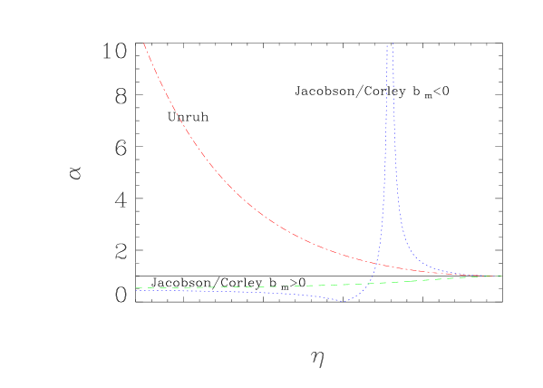
FIG. 3.: Sketch of the time evolution of the adiabaticity coefficient $\alpha$ for the dispersion relations.

We conclude that it is possible that in models of inflation based consistently on a unified theory at the Planck scale the predictions for fluctuations will not coincide with the usual predictions from our current inflationary Universe models. Generalizing from our results, a crucial issue appears to be whether the evolution of the quantum states corresponding to the fluctuations will be adiabatic on length scales smaller than the Planck scale.

Our results point to the possibility that the interaction between fundamental physics and cosmology may be much richer than hitherto assumed. It is not only a question of if and how fundamental physics leads to inflation; a much richer question is what the specific predictions of the fundamental model of inflation will be, assuming for the sake of argument that such a fundamental model exists.

It is not surprising that super-Planck-scale physics may modify the usual predictions of inflation. One model of the early Universe motivated by string theory, the Pre-Big-Bang Cosmology [34] based on dilaton gravity, leads to a super-exponential period of early evolution in which the Hubble constant is increasing, and where the predicted spectrum of scalar metric fluctuations is not scale-invariant [35]. It would be interesting to analyze the predictions of other models of inflation based on string theory, taking into account the evolution on string scales. One toy model in which this question could be analyzed is the nonsingular Universe [36] based on higher derivative terms in the gravitational action.

In the context of the models studied here, it would be interesting to explore whether the minimum energy density initial state is an attractor in a similar sense that the local Minkowski vacuum is in standard inflationary cosmology [28].

Note that models of inflation based on a strongly interacting theory (such as the model analyzed in [37]) do not suffer from the Trans-Planckian problem discussed in this paper. In strongly interacting theories, perturbations are generated at all times at a fixed physical scale, and a scale-invariant spectrum results based on the heuristic arguments mentioned in the Introduction. In such theories, however, the presence of strong interactions makes it hard to calculate the amplitude of the resulting spectrum.

Acknowledgements

We are grateful to Lev Kofman, Dominik Schwarz, Carsten Van de Bruck and in particular Bill Unruh for stimulating discussions and useful comments. We also thank an anonymous referee for useful comments. We acknowledge support from the BROWN-CNRS University Accord which made possible the visit of J. M. to Brown during which most of the work on this project was done, and we are grateful to Herb Fried for his efforts to secure this Accord. One of us (R. B.) wishes to thank Bill Unruh for hospitality at the University of British Columbia during the time when this work was completed. J. M. thanks the High Energy Group of Brown University for warm hospitality. The research was supported in part by the U.S. Department of Energy under Contract DE-FG02-91ER40688, TASK A.

REFERENCES

- [1] A. Guth, Phys. Rev. D23, 347 (1981).
-
[2]
G. Chibisov and V. Mukhanov, ‘Galaxy Formation and
Phonons,’ Lebedev Physical Institute Preprint No. 162 (1980);
V. Mukhanov and G. Chibisov, JETP Lett. 33, 532 (1981);
V. Mukhanov and G. Chibisov, Sov. Phys. JETP 56, 258 (1982);
G. Chibisov and V. Mukhanov, Mon. Not. R. Astron. Soc. 200, 535 (1982)
V. Lukash, Pis’ma Zh. Eksp. Teor. Fiz. 31, 631 (1980). -
[3]
W. Press, Phys. Scr. 21, 702 (1980);
K. Sato, Mon. Not. R. Astron. Soc. 195, 467 (1981). -
[4]
M. Sasaki, Prog. Theor. Phys. 76, 1036 (1986);
V. Mukhanov, Zh. Eksp. Teor. Fiz. 94, 1 (1988). - [5] V. Mukhanov, H. Feldman, and R. Brandenberger, Phys. Rep. 215, 203 (1992).
- [6] A. Starobinsky, Phys. Lett. 117B, 175 (1982).
- [7] S. Hawking, Phys. Lett. 115B, 295 (1982).
- [8] A. Guth and S. Y. Pi, Phys. Rev. Lett. 49, 1110 (1982).
- [9] J. Bardeen, P. Steinhardt, and M. Turner, Phys. Rev. D28, 679 (1983).
- [10] R. Brandenberger, Nucl. Phys. B245, 328 (1984).
-
[11]
E. Harrison, Phys. Rev. D1, 2726 (1970);
Ya. B. Zel’dovich, Mon. Not. R. astron. Soc. 160, 1 (1972). - [12] T. Bunch and P. C. W. Davies, Proc. Roy. Soc. Lond. A360, 117 (1978).
- [13] J. Martin, A. Riazuelo and M. Sakellariadou, Phys. Rev. D61, 083518 (2000). astro-ph/9904167.
-
[14]
A. Linde, D. Linde and A. Mezhlumian, Phys. Rev.
D49, 1783 (1994);
A. Linde, ‘Lectures on Inflationary Cosmology’, Stanford preprint SU-ITP-94-36, hep-th/9410082 (1994). - [15] T. Jacobson, hep-th/0001085.
- [16] S. Hawking, Comm. Math. Phys. 43, 199 (1975).
-
[17]
T. Jacobson, Phys. Rev. D44, 1731 (1991);
T. Jacobson, Phys. Rev. D48, 728 (1993). - [18] W. Unruh, Phys. Rev. D51, 2827 (1995).
- [19] R. Brout, S. Massar, R. Parentani and P. Spindel, Phys. Rev. D52, 4559 (1995).
- [20] N. Hambli and C. Burgess, Phys. Rev. D53, 5717 (1996)
-
[21]
S. Corley and T. Jacobson, Phys. Rev. D54, 1568 (1996);
S. Corley, Phys. Rev. D57, 6280 (1998). - [22] J. Kowalski-Glikman, Phys. Lett. 409B, 1 (2001).
- [23] M. Brown and C. Dutton, Phys. Rev. D18, 4422 (1978).
- [24] E. M. Lifshitz amd I. M. Khalatnikov, Adv. Phys. 12, 185 (1963).
- [25] L. P. Grishchuk, Phys. Rev. D 50, 7154 (1994).
- [26] L. P. Grishchuk, Zh. Eksp. Teor. Fiz 67, 825 (1974).
- [27] J. Martin and D. Schwarz, Phys. Rev. D57, 3302 (1998).
- [28] R. Brandenberger and C. Hill, Phys. Lett. 179B, 30 (1986).
- [29] L. Landau and E. M. Lifshitz, Hydrodynamics, Vol. 6, p. 432, Mir (1972).
- [30] C. Schmid, D. J. Schwarz and P. Widerin, Phys. Rev. D 59, 043517 (1999).
- [31] I. S. Gradshteyn and I. M. Ryzhik, Tables of Integrals, Series and Products, Academic, New York, 1981.
- [32] R. Brandenberger and J. Martin, in preparation.
- [33] J. C. Niemeyer and R. Parentani, astro-ph/0101451.
-
[34]
M. Gasperini and G. Veneziano, Astropart. Phys. 1, 317 (1993);
J. Levin and K. Freese Phys. Rev. D47, 4282 (1993). - [35] R. Brustein, M. Gasperini, M. Giovannini, V. Mukhanov and G. Veneziano, Phys. Rev. D51, 7644 (1995).
- [36] V. Mukhanov and R. Brandenberger, Phys. Rev. Lett. 68, 1969 (1992).
- [37] R. Brandenberger and A. Zhitnitsky, Phys. Rev. D55, 4640 (1997).