ANL-HEP-PR-00-055

MIT-CTP-2986

hep-th/0005192

We examine the dual correspondence between holographic IIB superstring theory and ${\cal N}=4$ super Yang-Mills theory at finite values of the coupling constants. In particular we analyze a field theory strong-coupling expansion which is the S-dual of the planar expansion. This expansion arises naturally as the AdS/CFT dual of the IIB superstring scattering amplitudes given a genus truncation property due to modular invariance. The space-time structure of the contributions to the field theory four-point correlation functions obtained from the IIB scattering elements is investigated in the example of the product of four conserved stress tensors, and is expressed as an infinite sum of field theory triangle integrals. The OPE structure of these contributions to the stress tensor four-point function is analyzed and shown not to give rise to any poles. Quantization of the string in the background of a five-form field strength is performed through a covariantized background field approach, and relations to the ${\cal N}=4$ topological string are found.

1 Introduction

Holographic string scattering within the conjectured duality between ${\cal N}=4$ super Yang-Mills theory and IIB superstring theory [1, 2, 3] has led to many interesting results within the low-energy supergravity approximation of string theory. According to the Maldacena conjecture, the string theory parameters $\alpha^{\prime}$ and $g_{s}$, the inverse string tension and the string coupling, are related to the field theory parameters $N$ and $\lambda$, the number of colors and the ’t Hooft coupling, by

$${L^{4}\over\alpha^{\prime 2}}=\lambda=g^{2}_{\rm YM}N\,,\qquad\qquad g_{s}={1\over 4\pi}\,g^{2}_{\rm YM}\ ,$$ (1.1)

where $L$ is the AdS radius. The supergravity approximation to string theory is valid if the string coupling is small and if the inverse string tension is much smaller than the square of the AdS radius. In the dual field theory this regime pertains to both $N$ and $\lambda$ very large with $g_{\rm YM}$ small. In this approximation a variety of ${\cal N}=4$ super Yang-Mills theory correlation functions have been calculated and properties of the strong coupling limit of the gauge theory found using the AdS/CFT correspondence (an exhaustive list of references may be found in [4]). Non-trivial renormalization properties of the correlation functions, as well as the correspondence between field theory operators and string states, provide evidence for the AdS/CFT correspondence. For correlation functions satisfying a non-renormalization theorem, such as two- and three-point functions involving conserved currents or scalar chiral primary operators, these results have been used successfully to test the AdS/CFT correspondence by finding agreement between the strong coupling AdS results and weak coupling perturbative field theory calculations [5, 6, 7, 8, 9, 10]. Further non-trivial tests of the correspondence in the supergravity approximation are provided by non-renormalization theorems for extremal $n$-point correlation functions with $n\geq 4$ and by non-trivial renormalization properties of related correlators [11, 12, 13, 14, 15].

However holographic string scattering, as formulated in [3], provides a generating functional also for finite values of the coupling constant. By virtue of the AdS/CFT duality, this formulation provides additional constraints on both string and field theory given that the AdS/CFT duality holds at finite values of the couplings. The OPE structure of ${\cal N}=4$ super Yang-Mills theory is directly related to the string scattering, and also to the truncation of the string theory to its massless modes in a string-inspired regulated supergravity context as discussed in [16].

A natural extension of the supergravity limit investigations towards the intermediate coupling regime is to relax the conditions of the supergravity low-energy limit and to consider string contributions to the correlation functions. This amounts to investigating the consequences of the duality in its “strong” form, i.e. to assume its validity for any value of $N$ and $\lambda$, and to analyzing its consequences both for the boundary field theory and for the superstring itself. A first step is the consideration of corrections to the massless mode scattering of supergravity in an expansion in the inverse string tension and in the string coupling in the holographic context [17], as opposed to a direct path integral quantization in the five-form background. This weakly coupled parameter region of string theory with $\alpha^{\prime}$ and $g_{s}$ small corresponds on the field theory side to the parameter region where

$$\lambda=g_{\rm YM}^{2}N\;\;\;\;{\rm large}\,,\;\;\;\;\;\;\;\;g_{\rm YM}^{2}=\frac{\lambda}{N}\;\;\;\;{\rm small}\,.$$ (1.2)

For the stress tensor four-point function, the first non-trivial $\alpha^{\prime}$ correction was considered in [17] with regards to instantons within the AdS/CFT correspondence. On the string theory side, this correction is given by [18]

$$S^{IIB}=\frac{1}{{\alpha^{\prime}}^{4}}\,\int\!{\rm d}^{10}x\;\sqrt{-g}\,{\alpha^{\prime}}^{3}\,e^{-\phi/2}\,f^{0}(\tau,\bar{\tau})t^{8}t^{8}R^{4}\,,$$ (1.3)

where $R$ is the curvature tensor contracted in the way well-known from the tree and genus one scattering amplitude in IIB string theory. The tensor $t^{8}$ and its contraction with $R^{4}$ will be given in more detail below. $f^{0}(\tau,\bar{\tau})$ is a non-holomorphic Eisenstein series, $E_{3/2}(\tau,\bar{\tau})$, whose form is strongly constrained by the $SL(2,Z)$ invariance of IIB superstring graviton scattering. In the quantum supergravity limit where string modes are absent there is a piece of this structure that remains upon specification of the string-related regulator of the supergravity. Furthermore in the classical limit of supergravity, there is a $SL(2,R)$ symmetry which has implications for ${\cal N}=4$ super Yang-Mills at infinite $N$ and $\lambda$, as discussed discussed in detail in [19, 20]. To the derivative order given by (1.3), the low-energy scattering of gravitons (and of the other fields of the string) receives tree and genus one contributions from the string perturbation expansion in $g_{s}$, as well as non-perturbative contributions from D instantons. Within AdS/CFT, the argument $\tau$ in (1.3) is related to the Yang-Mills variables by

$$\tau={\theta\over 2\pi}+i{4\pi\over g_{\rm YM}^{2}}\,.$$ (1.4)

$f^{0}(\tau,\bar{\tau})$ has the correct coupling constant dependence to agree with field-theory instanton calculations.

In [17] it was shown that $AdS_{5}\times S_{5}$ remains a solution of the string theory equations of motion in the presence of the term (1.3) to all orders in $g_{s}$. This is essentially due to the symmetry properties of the $t^{8}$ tensors which ensure that only the Weyl tensor part of the curvature tensors contributes to (1.3). Since the space $AdS_{5}\times S_{5}$ is conformally flat, its Weyl tensor vanishes. The space-time dependence of the four-point function contribution obtained from the four-dilaton term in the low-energy S-matrix in (1.3) was calculated in [21], where it was shown for holographic dilaton scattering that its short-distance singularities are at most logarithmic.

On the string theory side, several extensions of (1.3) to higher orders in $\alpha^{\prime}$ have been discussed. These include terms involving the five-form field strength $F_{5}$ [22], a direct $SL(2,Z)$ covariantization of the IIB tree-level graviton scattering involving derivatives acting on the $R^{4}$ structure [24, 25], as well perturbation theory based on a manifest $SL(2,Z)$ invariant theory [26]. The $\Box^{2}R^{4}$ next to leading term was analyzed at genus two in [27]. Supersymmetry constraints on the string expansion to lowest order were investigated in [28]. In all of these cases $S$-duality or modular invariance play a crucial role in determining the coupling dependence in terms of Eisenstein series (See also [29, 30]). For graviton scattering, an extension of the S-matrix that is compatible with perturbative string theory and the known results in maximal supergravity, as well as with unitarity of the massless sector, has been given in [16].

Via the AdS/CFT correspondence, all of these string theory scattering amplitudes give rise to contributions to the stress tensor four-point function at strong ’t Hooft coupling. The $\lambda$ and $N$ dependence of these contributions corresponds to a resummation of the perturbative series as well as to a ’t Hooft expansion around an instanton background. The fact that the coupling dependence of the string theory amplitudes is strongly constrained by modular invariance implies on the field theory side that the ’t Hooft large $N$ expansion, for which

$$\lambda=g_{\rm YM}^{2}N\;\;\;\;{\rm small\;and\;fixed}\,,\;\;\;\;\;\;\;\;N\rightarrow\infty\,,\;\;$$ (1.5)

has only a finite number of perturbative terms in $\lambda$ at each order in $N$, considered for the instantonic terms in [31]. Of course, the derivation of this result requires the assumption that the large $\lambda$ expression obtained from string theory may be analytically continued to the weak coupling regime determined by the ’t Hooft limit (1.5). The instanton sector non-renormalization theorem following from this assumption, where “non-renormalization” means that there are only finitely many perturbative terms for a given order in $1/N$, is consistent with the results of [32, 33, 34], where instanton contributions are calculated to leading order in $\alpha^{\prime}$. We refer the reader to [35] for a comprehensive review.

In this paper we consider the extension of the IIB superstring S-matrix to all orders in $\alpha^{\prime}$ and $g_{s}$ given in [16]. By virtue of the AdS/CFT correspondence we examine its consequences for ${\cal N}=4$ super Yang-Mills theory. In the superstring theory, there are, for example, higher derivative terms in the covariantized S-matrix which are generated by

$$S_{4-pt}^{\rm IIB}=\frac{1}{\alpha^{\prime}}\sum_{k=0}^{\infty}\int d^{10}x\sqrt{g}~{}\alpha^{\prime}{}^{k}\,f_{k}(\tau,\bar{\tau})\Box^{k}R^{4}\ \,.$$ (1.6)

Here $\Box^{k}R^{4}$ is a shorthand notation for derivatives acting on some of the curvature tensors. The $\Box^{k}R^{4}$ terms have the same supersymmetry weight as the $R^{4}H^{4k}$ amplitudes of the ${\cal N}=4$ topological string [36]. As discussed in [16], the functions $f_{k}$ in (1.6) are again severely constrained by modular invariance, which strongly suggests in particular that at order $k$ in $\alpha^{\prime}$, there are only finitely many perturbative corrections up to a maximum genus $g_{\rm max}={1\over 2}(k+2)$ for $k$ even or $g_{\rm max}={1\over 2}(k+1)$ for $k$ odd. We refer to this behaviour as the genus truncation property.

Using the strong form of the AdS/CFT correspondence, we calculate the contributions to the stress tensor four point function arising from (1.6) and from further polynomial terms in the string scattering elements. We derive the $\lambda$ and $N$ dependence of these contributions from the functions $f_{k}$ using the relations (1.1). A further essential ingredient of our analysis, motivated by the importance of modular invariance in this context, is to reorganize the series for the coupling dependence into terms involving the S-dual of the ’t Hooft coupling $\lambda$. Under $S$-duality we have $g_{\rm YM}\rightarrow 1/g_{\rm YM}$ such that

$$\lambda=g^{2}_{YM}N\,\;\;\;\;\rightarrow\,\;\;\;\;\lambda_{D}=\frac{N}{g^{2}_{\rm YM}}=\frac{N^{2}}{\lambda}\,.$$ (1.7)

Furthermore the S-dual of the original ’t Hooft limit (1.5) is given by

$$\lambda_{D}=\frac{N^{2}}{\lambda}\,\;\;\;\;{\rm small\;and\;fixed}\,,\;\;\;\;\;\;\;\;N\rightarrow\infty\,.$$ (1.8)

From the point of view of the original ’t Hooft coupling $\lambda$ this is clearly a strong coupling limit since both $\lambda$ as well as the Yang-Mills coupling $g_{\rm YM}$ are very large in this limit.

We find that in this dual ’t Hooft limit the perturbation series in $\lambda_{D}$ arising from the modular functions $f_{k}$ contains just the terms corresponding to the highest genus contribution for each $\alpha^{\prime}$ on the string theory side, given that the genus truncation property holds. This leads us to the result that given the strong form of the AdS/CFT correspondence, the genus truncation property is equivalent to the convergence of the strong coupling perturbative expansion of ${\cal N}=4$ SYM in $\lambda_{D}$ in the dual ’t Hooft limit.

Since $g_{\rm YM}$ is no longer small in the dual ’t Hooft limit we are outside the parameter region given by (1.2). We do not prove the convergence of the S-dual to the planar series here. However the original proof of the convergence of the planar series in $\lambda$ [38], according to which the planar expansion has a finite radius of convergence, in combination with the strong implications of S-duality, provides a strong argument in favour of the convergence of the $\lambda_{D}$ series in the dual ’t Hooft limit.

Furthermore, we determine the spatial dependence of the contributions to the stress tensor four-point function arising from (1.6), which correspond to contact diagrams for the graviton scattering, and investigate their short-distance limit when two of the four point approach each other. In particular, we show that (1.6) does not contribute any leading terms to the OPE. This implies that there are no poles, which is consistent with the instanton nature of (1.6), and also with Ward identities relating the four-point function to the three-point function for which a non-renormalization theorem holds. Another consequence is that these contact contributions to the stress tensor four-point function do not contain any term which factors into two two-point functions (in contrast to the exchange contributions, which also contribute non-trivially to the Ward identities).

The outline of this work is as follows. In section 2 we examine the generating function of correlation functions given by the holographic string scattering of gravitons dual to the composite stress-tensor operators. We analyze the coupling constant structure and re-organize the planar expansion into its S-dual relative. In section 3 we examine the latter series and convergence with regards to the modular properties of the string scattering. In section 4 we derive a generating functional as a one-parameter integral representation that resums an infinite class of known contributions of the string scattering (with similar resummations in integral form). We also examine the unitarity structure of the holographic scattering with regards to the correlation functions in the dual gauge theory. The space-time structure of the correlation functions are examined in section 5, and using conformal inversions, the holographic contact diagrams are expressed as triangle one-loop integral functions. The tensor structure is obtained by extracting appropriate derivatives. We also consider related box diagrams relevant for contact diagrams as well as for massless supergravity exchange diagrams. The pole structure of the finite coupling constant dual correlators is examined and shown to be sub-leading away from the infinite coupling limit when only the contact diagrams contribute. In section 7 we conclude and discuss related avenues.

2 ${\cal N}=4$ Correlation functions from IIB Quantum S-matrix

In this section we examine the $\alpha^{\prime}$ and $g_{s}$ expansion of IIB superstring theory in the background of the $AdS_{5}\times S^{5}$ space with regards to deriving the super Yang-Mills theory correlators and their coupling dependence. We begin by discussing terms in the $\alpha^{\prime}$ expansion which lead to contact diagrams for the four-graviton scattering. Then we discuss terms in the expansion which lead to exchange diagrams. Subsequently we show how Yang-Mills correlators are obtained by virtue of the AdS/CFT correspondence and discuss their coupling dependence in detail, in particular the implications of the genus truncation property.

As discussed in [16], the low-energy derivative expansion of the IIB superstring S-matrix in ten-dimensions for energies such that $s<4/\alpha^{\prime}$ involves contributions of the form

$$S_{4-pt}^{\rm IIB}=\sum_{k=0}^{\infty}{1\over\alpha^{\prime}}\int d^{10}x\sqrt{g}~{}f_{k}(\tau,\bar{\tau})(\alpha^{\prime}\Box)^{k}R^{4}\$$ (2.1)

in Einstein frame and where $f_{k}(\tau,\bar{\tau})$ are invariant non-holomorphic functions under fractional linear transformations of the IIB string coupling constant $\tau=\chi+ie^{-\phi}$, which we label as $\tau=\tau_{1}+i\tau_{2}$. The individual terms in (2.1) are

$$\Box^{k}R^{4}\rightarrow t^{8}_{\mu_{1}\nu_{1}\ldots\mu_{4}\nu_{4}}t^{8}_{{\bar{\mu}}_{1}{\bar{\nu}}_{1}\ldots{\bar{\mu}}_{4}{\bar{\nu}}_{4}}\Box^{k}\Bigl{(}R^{\mu_{1}\nu_{1}{\bar{\mu}}_{1}{\bar{\nu}}_{1}}R^{\mu_{2}\nu_{2}{\bar{\mu}}_{2}{\bar{\nu}}_{2}}\Bigr{)}R^{\mu_{3}\nu_{3}{\bar{\mu}}_{3}{\bar{\nu}}_{3}}R^{\mu_{4}\nu_{4}{\bar{\mu}}_{4}{\bar{\nu}}_{4}}\ ,$$ (2.2)

together with mixed derivatives on the curvature tensors (at tree-level in momentum space the tensor has the form $s^{k}+t^{k}+u^{k}$). The expansion in (2.1) pertains to the four-point graviton scattering amplitude; higher $n$-point amplitudes involve further curvature tensors (related to additional polarization vectors). The generic $R^{4}$ structure has not been explicitly shown to be the unique tensor at higher-genus, although there is evidence based on multi-loop IIB supergravity scattering [39] as well as in multi-genus superstring scattering; further symmetry structures of the indices constrain the possible forms, as discussed below. We consider the generic $R^{4}$ tensor structure to be a consequence of ${\cal N}=8$ supersymmetry. In momentum space, $\Box^{k}$ represents the symmetrized factor

$$\Box^{k}\rightarrow s^{k}+t^{k}+u^{k}\ ,$$ (2.3)

with the invariants

$$s=(k_{1}+k_{2})^{2}\qquad t=(k_{1}+k_{3})^{2},\qquad u=(k_{2}+k_{3})^{2}$$ (2.4)

at tree-level, and more general (unknown) combinations $s^{k_{1}}t^{k_{2}}u^{k_{3}}$ (with $k_{1}+k_{2}+k_{3}=k$) at higher-genus. Note that $s+t+u=0$ and $s^{3}+t^{3}+u^{3}=3stu$ via momentum conservation.

Furthermore, the R$\otimes$R five-form effects coupled with the $R^{4}$ have the expansion

$$S^{F}_{4-pt}=\sum_{k=1}^{\infty}{1\over\alpha^{\prime}}\int d^{10}x\sqrt{g}~{}g_{k}(\tau,\bar{\tau})\alpha^{\prime 2k}F_{5}^{4k}R^{4}\ .$$ (2.5)

Consistent classical propagation of the string requires the beta function conditions

$$\langle R_{\mu\nu}\rangle=e^{\phi}\langle F_{5,\mu}{}^{\mu_{1}\ldots\mu_{4}}F_{5,\nu\mu_{1}\ldots\mu_{4}}\rangle\ ,$$ (2.6)

and we take this to hold at higher order (potential corrections at higher order in $\alpha^{\prime}$, i.e. at four loops, potentially produce an $R^{4}$ counterterm which vanishes in the background as required by stability).

The tree-level coefficient in (2.5) in string frame has the coupling constant

$$g_{k}^{\rm tree}=\tau_{2}^{-5k+2}$$ (2.7)

with successive $\tau_{2}^{-2}$ at higher genus; the conjecture in [22, 23] generates the form of (2.5) at genus zero and genus $k-1$ for a given $k$. Lastly, a multi-point graviton scattering amplitude generates terms in the quantum generating functional of the S-matrix of the form

$$S^{4+n;k}=\sum_{i_{n}=1}^{\infty}{1\over\alpha^{\prime}}\int d^{10}x\sqrt{g}~{}h^{(n)}_{i_{n}}(\tau,\bar{\tau})(\alpha^{\prime})^{2k+n}F_{5}^{4k}R^{4+n}\ ,$$ (2.8)

where a tensor contraction of the curvature tensors is implied and may be found by performing amplitude calculations in the IIB superstring. The analysis of the coupling constant structure of these terms in (2.8) and (2.5) is similar to that in (2.1).

In the background field approach, the substitution of the $AdS_{5}\times S^{5}$ metric into (2.8) leads to a contraction of four $R_{\mu\nu}$ terms in the expansion, and the question arises as to how many independent tensors this term may generate. The Weyl symmetries and those of the four-graviton scattering permit in general three independent tensors, and requiring stability of the background implies that the contribution of the higher-derivative term in (2.8) gives rise to the same $R^{4}$ term as before but with a coupling constant structure associated with the higher derivatives. The form has an overall factor of

$${1\over L^{2n+4k}}\alpha^{\prime 2k+n}={1\over\lambda^{k+n/2}}\ ,$$ (2.9)

in addition to the relative higher string coupling constants associated with the genus corrections in $h^{(n)}(\tau,\bar{\tau})$.

The form in (2.5) and in (2.1) may be found by performing explicit S-matrix calculations in IIB superstring theory. In (2.5) a background value $\langle F_{5}\rangle$ and $g_{\mu\nu}^{AdS}$ ($\langle R^{\mu\nu}{}_{\rho\gamma}\rangle$) generates additional contributions in the covariantized scattering to those obtained from that in (2.1) within the AdS/CFT correspondence. Note that in the on-shell quantum corrected effective action there is no requirement to have an off-shell IIB description of the action for the self-dual five-form.

In addition to (2.5) and (2.1) which lead to contact bulk four-point interactions for gravitons on the anti-de Sitter space, there are also exchanges of the massless modes at tree-level. They contribute a term of the form

$$S_{m=0}^{4-pt,IIB}={1\over\alpha^{\prime}}\int d^{10}x\sqrt{g}~{}{1\over(\alpha^{\prime}\Box)^{3}}R^{4}\ ,$$ (2.10)

to the quantum corrected on-shell action found from the S-matrix. Here the inverted $\Box$’s are arranged so that in momentum space the factor $stu$ is found. In the holographic context these exchange contributions have been analyzed in a number of works and correspond to the infinite $N$ and $\lambda$ results. There are further non-analytic terms in the S-matrix related to the thresholds of the massless modes and unitarity, which may be constructed iteratively following the analysis in [16] from the $SL(2,Z)$ construction of matrix elements in IIB superstring theory.

We now investigate the coupling dependence of these S-matrix contributions. The functional form in (2.1) represents the polynomial terms that arise from integrating out the massive modes at genus $g\geq 0$ and the massless ones at $g\geq 1$ in the genus expansion (in the string field theory this arises in a well-specified regulator). An ansatz for the functional form of $f_{k}(\tau,\bar{\tau})$ using Eisenstein series has been proposed in [16]. The general perturbative structure of $f_{k}(\tau,\bar{\tau})$ required by the dilaton dependence of IIB superstring perturbation theory is

$$f_{k}(\tau,\bar{\tau})=a_{0}^{(k)}\tau_{2}^{{3\over 2}+{k\over 2}}+a_{1}^{(k)}\tau_{2}^{-{1\over 2}+{k\over 2}}+a_{2}^{(k)}\tau_{2}^{-{5\over 2}+{k\over 2}}+\ldots\ ,$$ (2.11)

which is a decreasing power series in the string coupling constant $\tau_{2}^{2}$. In (2.11), the index $k$ labels the order in $\alpha^{\prime}$ (twice the number of derivatives with respect to the eight derivative $R^{4}$ term) and the subscript on $a_{i}$ the contributing genus order. In [16] it was conjectured that this series truncates, i.e. for a given $k$ the S-matrix receives perturbative corrections up to a maximum genus $g_{\rm max}={1\over 2}(k+2)$ ($k$ even) and $g_{\rm max}={1\over 2}(k+1)$ ($k$ odd). The corresponding set of terms in the low-energy expansion is listed in Table 1. This genus truncation is in agreement with the modular structure of S-duality, together with the perturbative dependence in uncompactified IIB string theory together with further consistency conditions of the S-matrix. Furthermore, it is in agreement with the genus truncation of the conjectures for the amplitudes $R^{4}H^{4g-4}$ in [22]. The non-analytic terms in the superstring S-matrix contribute orders in the derivative expansion below the starred entries in Table 1. The leading primitive divergences of the supergravity are polynomials in momenta, with the non-analytic terms non-leading. In ${\cal N}=4$ super Yang-Mills theory these terms will therefore contribute only at sub-leading in $N$.

Table 1: Example contributions to $\Box^{k}R^{4}$ arising in string perturbation theory at genus $g$. The asterisk denotes the top genus contributions.

	$g=0$	$g=1$	$g=2$	$g=3$	$g=4$	$\ldots$
$R^{4}$	$\surd$	$\surd^{\star}$
$\Box R^{4}$
$\Box^{2}R^{4}$	$\surd$		$\surd^{\star}$
$\Box^{3}R^{4}$	$\surd$	$\surd$	$\surd$
$\Box^{4}R^{4}$	$\surd$	$\surd$	$\surd$	$\surd^{\star}$
$\Box^{5}R^{4}$	$\surd$	$\surd$	$\surd$	$\surd$
$\Box^{6}R^{4}$	$\surd$	$\surd$	$\surd$	$\surd$	$\surd^{\star}$
$\cdots$

From the expansion in (2.1) we may derive quantum corrected equations of motion and generate the finite $\lambda$ and $N$ terms in the boundary ${\cal N}=4$ gauge theory; in the following we consider the contributions from (2.1) for simplicity. The remaining terms in (2.8) may be analyzed in a similar way, and we shall comment on their contributions to the analysis when appropriate.

For obtaining the contribution of (2.1) to the stress tensor four-point function, we consider fluctuations around the background geometry $AdS_{5}\times S_{5}$ and vary four times with respect to the five-dimensional fluctuation around $AdS_{5}$. Then we restrict to $AdS_{5}\times S_{5}$. The five-sphere contributes just a constant factor which we omit in the subsequent.

For the $AdS_{5}$ geometry we use the conventions and notations of [5]. In particular, for the square of the five-dimensional line element we have $ds^{2}={1\over z_{0}^{2}}(dz_{0}^{2}+d{\vec{z}}^{2})$, where $z_{0}\geq 0$ and ${\vec{z}}\in R^{d}$. The background solution for the $AdS_{5}$ compactification is

$$F_{\mu_{1}\ldots\mu_{5}}={1\over L}\epsilon_{\mu_{1}\ldots\mu_{5}}\qquad R_{\mu_{1}\ldots\mu_{4}}={1\over L^{2}}\bigl{(}g_{\mu_{1}\mu_{3}}g_{\mu_{2}\mu_{4}}-g_{\mu_{1}\mu_{4}}g_{\mu_{2}\mu_{3}}\bigr{)}\ .$$ (2.12)

The curvature of the AdS space, $L$, is set to unity unless otherwise stated. The form in (1.1) translates tree exchange of the modes of the superstring and the higher genus orders in the holographic string theory on $AdS_{5}\times S^{5}$ to $\lambda$ and $N^{2}$ effects, respectively, in the ${\cal N}=4$ gauge theory.

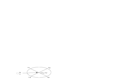
Figure 1: Holographic effective four-point contact diagram found from the covariantized fourth variation of the on-shell IIB string scattering element. The $\Box$ denotes the action $\Box^{k}R^{4}$.

In this way we obtain for the effective four-point vertex

$$V_{g}^{(k),\{\mu_{i}\nu_{i}\}}(z_{0},{\vec{z}})\equiv a_{g}^{(k)}\tau_{2}^{3/2+k/2-2g}\alpha^{{}^{\prime}k+3}~{}\prod_{j=1}^{4}\bigl{\{}{\delta\over\delta{\hat{g}}(z_{0},{\vec{z}})}\bigr{\}}\Bigl{[}\sqrt{g}~{}\Box^{k}R^{4}\Bigr{]}|_{g_{AdS_{5}\times S^{5}}}\ ,$$ (2.13)

$$=a_{g}^{(k)}\tau_{2}^{3/2+k/2-2g}\alpha^{{}^{\prime}k+3}~{}{\tilde{V}}_{g}^{(k),\{\mu_{i}\nu_{i}\}}(z_{0},{\vec{z}})\ ,$$ (2.14)

where ${\hat{g}}$ is the fluctuation around the background geometry and $a_{g}^{(k)}$ is a numerical constant related to the genus $g$ and order $\alpha^{\prime k}$ term in the expansion at small $\alpha^{\prime}$. The vertex in (2.13) generates the holographic Feynman-Witten diagram in Figure 1 and is dual to the contribution to the correlation of four stress-tensors by virtue of

$$\langle\prod_{j=1}^{4}T^{a_{j}b_{j}}({\vec{x}}_{i})\rangle=N^{2}\sum_{k=0}^{\infty}\sum_{g=0}^{g_{k}}\lambda^{-k/2}\Bigl{(}{\lambda\over N}\Bigr{)}^{-3/2+2g}a_{g}^{(k),\{a_{j}b_{j}\}}({\vec{x}}_{i})$$ (2.15)

$$a_{g}^{(k),\{a_{i}b_{i}\}}({\vec{x}}_{i})=a_{g}^{(k)}~{}\int{dz_{0}d^{d}{\vec{z}}\over z_{0}^{d+1}}~{}\Bigl{[}\prod_{i=1}^{4}G^{\{a_{i}b_{i}\}}{}_{\{\mu_{i}\nu_{i}\}}({\vec{x}}_{i};z_{0},{\vec{z}})\Bigr{]}~{}{\tilde{V}}_{g}^{(k),\{\mu_{i}\nu_{i}\}}(z_{0},{\vec{z}})\ ,$$ (2.16)

for ${\cal N}=4$, $d=4$ ($AdS_{d+1}$). Here $G^{ab}{}_{\mu\nu}({\vec{x}}_{i};z_{0},{\vec{z}})$ is the appropriate bulk-boundary kernel. The space-time dependence of (2.15) is discussed in detail in Section 5 below.

We shall suppress the external graviton indices associated with the bulk-boundary kernel,

$$a_{k}^{(g)}({\vec{x}}_{i})=a_{k}^{(g),\{a_{j}b_{j}\}}({\vec{x}}_{i})\ ,$$ (2.17)

when it is clear from the text. Furthermore we define

$$\langle\prod_{j=1}^{4}T^{a_{j}b_{j}}({\vec{x}}_{i})\rangle=N^{2}~{}\sum_{k=1}^{\infty}\sum_{g=0}^{g_{k}}f_{g}^{(k),\{a_{j}b_{j}\}}({\vec{x}}_{j})\ ,$$ (2.18)

where $g$ labels the genus order and $(k)$ the derivative order ($k=0$ corresponds to eight derivatives) in the genus expansion. We define the the functions $f$ without an overall factor of $N^{2}$ and note that they express both the coupling dependence as well as the space-time structure. The space-time indices in (2.18) will be suppresssed in the subsequent discussion of the coupling dependence. Furthermore we define

$$f^{(k)}=\sum_{g=0}^{g_{k}}f_{g}^{(k)}\ ,$$ (2.19)

and

$$f_{g}=\sum_{k_{\rm min}}^{\infty}f^{(k)}_{g}\,,\quad\quad k_{\rm min}=2(g_{\rm max}-1)\,,$$ (2.20)

where $g_{\rm max}$ is the maximum even genus in agreement with the genus truncation property as defined in the introduction. Low-energy holographic scattering in the bulk string corresponds in the dual gauge theory to a power series in the coupling around infinite $\lambda$. Integrating out modes in the string and fixing energy scales of the scattering at lower values (hence probing larger distances) does not correspond to energy scales in the dual field theory but rather the region in coupling space accessible in the approximation around infinite coupling; this translates the Wilsonian sense of energy scales to the boundary data and we must integrate out to more orders in the bulk to access finite coupling in the dual gauge theory.

The massless graviton exchange given by (2.10) represents the supergravity approximation and has the coupling constant structure to be the leading $N$ and $\lambda$ contribution to the four-point correlation function. Its general form for the massless field exchange has been found in a number of recent papers [40, 41, 42, 43, 44], and generically corresponds to coordinate space box diagrams in the boundary field theory with rational function coefficients in the position variables. Contact diagrams arising from integrating massive string exchange diagrams produces similar box integrals, although in this case the results are found both by performing an $\alpha^{\prime}$ expansion at higher genus as well as at genus zero as far as the massive modes are concerned. We find that the field theory box structure appears generically to all orders in $\lambda$ and $N$ in this approach, including the integration over the massless propagating modes, as illustrated in Figure 2.

We shall step through the expansion in (2.15) to demonstrate the coupling structure from the point of view of IIB superstring theory and the regrouping of the terms in the S-dual variable. The general form of the large $\lambda$ and $N$ expanded correlation functions is found by using the covariantized S-matrix in (2.1) to leading order in $N^{2}$ through the $\alpha^{\prime}$ expansion. Using the $\tau_{2}^{2}$ expansion of (2.1), we list explicitly the functional dependence arising from $\Box^{k}R^{4}$ for $k=0$ through $k=4$ in the ${\cal N}=4$ gauge theory: From the $R^{4}$ term we have, using the notation (2.19),

$$f^{(0)}({\vec{x}}_{i}) = {1\over\lambda^{3/2}}\Bigl{[}a_{0}^{(0)}({\vec{x}}_{i})+a_{1}^{(0)}({\vec{x}}_{i})\Bigl{(}{\lambda\over N}\Bigr{)}^{2}\Bigr{]}\ ,$$ (2.21)

with $a_{0}^{(0)}$ the genus zero and $a_{1}^{(1)}$ the genus one terms of the gauge theory. The $\Box R^{4}$ vanishes on-shell due to momentum conservation, and the next ones are, from $\Box^{2}R^{4}$,

$$f^{(2)}({\vec{x}}_{i}) = {1\over\lambda^{5/2}}\Bigl{[}a_{0}^{(2)}({\vec{x}}_{i})+a_{2}^{(2)}({\vec{x}}_{i})\Bigl{(}{\lambda\over N}\Bigr{)}^{4}\Bigr{]}\ ,$$ (2.22)

from $\Box^{3}R^{4}$,

$$f^{(3)}({\vec{x}}_{i}) = {1\over\lambda^{3}}\Bigl{[}a_{0}^{(3)}({\vec{x}}_{i})+a_{1}^{(3)}({\vec{x}}_{i})\Bigl{(}{\lambda\over N}\Bigr{)}^{2}+a_{2}^{(3)}({\vec{x}}_{i})\Bigl{(}{\lambda\over N}\Bigr{)}^{4}\Bigr{]}\ ,$$ (2.23)

and from $\Box^{4}R^{4}$,

$$f^{(4)}({\vec{x}}_{i})={1\over\lambda^{7/2}}\Bigl{[}a_{0}^{(4)}({\vec{x}}_{i})+a_{1}^{(4)}({\vec{x}}_{i})\Bigl{(}{\lambda\over N}\Bigr{)}^{2}+a_{2}^{(4)}({\vec{x}}_{i})\Bigl{(}{\lambda\over N}\Bigr{)}^{4}+a_{3}^{(4)}({\vec{x}}_{i})\Bigl{(}{\lambda\over N}\Bigr{)}^{6}\Bigr{]}\ .$$ (2.24)

The general dependence from (2.1) is

$$f^{(k)}({\vec{x}}_{i})=\lambda^{-3/2-k/2}~{}\sum_{g=1}^{g_{\rm max}(k)}a_{g}^{(k)}({\vec{x}}_{i})\bigl{(}{\lambda\over N}\bigr{)}^{2g}\ .$$ (2.25)

In the above we assumed the genus truncation property to hold, but we shall analyze possible higher order contributions in the next section.

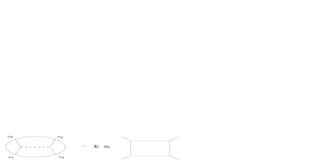
Figure 2: Massless field exchange produces linear combinations of box diagrams with rational function coefficients $a_{j}$.

We now rearrange the series in (2.25) in a manner so that the $N^{2}$ dependence is manifest. The leading $N$ dependence is captured by the first term in every series listed in (2.25). We use the notation (2.20). In the classical string theory limit we have, expanding in the string scale

$$f_{0}({\vec{x}}_{i})={1\over N^{3}}\Bigl{(}{N^{2}\over\lambda}\Bigr{)}^{3/2}\Bigl{[}a_{0}^{(0)}({\vec{x}}_{i})+{1\over\lambda}a_{0}^{(2)}({\vec{x}}_{i})+{1\over\lambda^{3/2}}a_{0}^{(3)}({\vec{x}}_{i})+{1\over\lambda^{2}}a_{0}^{(4)}({\vec{x}}_{i})+\ldots\Bigr{]}\ .$$ (2.26)

Sub-leading $N^{2}$-suppressed contributions are taken from the non-leading functions in (2.25). Each sub-leading series contains an infinite number of terms and are explicitly, from genus one,

$$f_{1}({\vec{x}}_{i})={1\over N}\bigl{(}{\lambda\over N^{2}}\bigr{)}^{1/2}\Bigl{[}a_{1}^{(0)}({\vec{x}}_{i})+{1\over\lambda^{3/2}}a_{1}^{(3)}({\vec{x}}_{i})+{1\over\lambda^{2}}a_{1}^{(4)}({\vec{x}}_{i})+{1\over\lambda^{5/2}}a_{1}^{(5)}({\vec{x}}_{i})+\ldots\Bigr{]}\ ,$$ (2.27)

from genus two,

$$f_{2}({\vec{x}}_{i})={1\over N}\bigl{(}{\lambda\over N^{2}}\bigr{)}^{3/2}\Bigl{[}a_{2}^{(2)}({\vec{x}}_{i})+{1\over\lambda^{1/2}}a_{2}^{(3)}({\vec{x}}_{i})+{1\over\lambda}a_{2}^{(4)}({\vec{x}}_{i})+{1\over\lambda^{3/2}}a_{2}^{(5)}({\vec{x}}_{i})+\ldots\Bigr{]}\ ,$$ (2.28)

and from genus three,

$$f_{3}({\vec{x}}_{i})={1\over N}\bigl{(}{\lambda\over N^{2}}\bigr{)}^{5/2}\Bigl{[}a_{3}^{(4)}({\vec{x}}_{i})+{1\over\lambda^{1/2}}a_{3}^{(5)}({\vec{x}}_{i})+{1\over\lambda}a_{3}^{(6)}({\vec{x}}_{i})+{1\over\lambda^{3/2}}a_{3}^{(7)}({\vec{x}}_{i})+\ldots\Bigr{]}\ .$$ (2.29)

The relative factors to the leading ones in the above series are

$${1\over\lambda^{1/2}}={1\over N}\Bigl{(}{N^{2}\over\lambda}\Bigr{)}^{1/2}\ ,$$ (2.30)

and for fixed $N^{2}/\lambda$ are $1/N$ suppressed as $N$ becomes large. The higher genus contributions have a factor of $N^{2}$ relative to the first series (i.e. classical superstring theory) in (2.26) after using the expansion in the dual coupling via (2.30); the classical string contribution is sub-leading in $N$ in the expansion of $\lambda/N^{2}$. Specific contributions are listed in (2.26)-(2.29). The perturbative series for the correlation function at large coupling $\lambda$ (and $N$) is encoded in the equation,

$$f_{j}({\vec{x}}_{i})=\lambda^{-1/2}\Bigl{[}{\lambda\over N^{2}}\Bigr{]}^{j}~{}\sum_{k=2j-2}^{\infty}\lambda^{-k/2}~{}a_{j}^{(k)}({\vec{x}}_{i})\ ,$$ (2.31)

where $j$ denotes the genus order and $k$ the $\alpha^{\prime}$ order in the low-energy expansion of the superstring graviton scattering.

In taking the dual ’t Hooft limit in (1.8) the perturbative series is re-organized and different terms in $f_{j}({\vec{x}}_{j})$ contribute. The strong coupling limit

$${\lambda\over N^{2}}={\rm fixed},\qquad N\rightarrow\infty\ ,$$ (2.32)

isolates from the sum of the functions $f_{j}({\vec{x}}_{i})$, or $f^{(k)}({\vec{x}}_{i})$, the leading dependence

$$\langle\prod_{j=1}^{4}T^{a_{j}b_{j}}({\vec{x}}_{i})\rangle|_{S-dual}=N^{2}\lambda^{-1/2}~{}\sum_{g=1}^{\infty}\Bigl{(}{\lambda\over N^{2}}\Bigr{)}^{g}a_{g}^{(2g-2),\{\mu_{j}\nu_{j}\}}({\vec{x}}_{j})\ .$$ (2.33)

The remainder to (2.33) has terms of order ${1\over\lambda^{1/2}}={1\over N}({N^{2}\over\lambda})^{1/2}$ higher and are individually suppressed in this limit. A similar expansion in $1/N$ is available by collecting the terms in (2.31) at lower orders in $\lambda$. The series in (2.33) does not contain terms in tree-level string scattering in the background, and as such does not have a classical supergravity limit.

The important aspect of the series in (2.33) in the string context is that for every $\alpha^{\prime}$ it just involves the maximum even genus contribution in agreement with the genus truncation property of [16], which is defined after (1.6) of the present paper. On the Yang-Mills side, (2.33) is an expansion in the S-dual of the ’t Hooft coupling to leading order in $1/N$. We see that a field theory proof of the convergence of the expansion in (2.33) would imply the genus truncation property in string theory. Vice-versa, a string theory proof of the genus truncation property would imply the convergence of the field theory strong coupling expansion. We note that ’t Hooft’s original proof of the convergence of the large $N$ planar expansion holds for a finite radius of convergence; together with the S-duality between the original planar expansion and the one considered here this provides strong evidence for the possibility of a field theory proof for the convergence of (2.33). The limit in (2.32) describes the dual planar limit of ${\cal N}=4$ gauge theory, and hence the monopole and dyonic dual description to the planar expansion in $1/N$.

From the weak coupling point of view, the limit in (2.32) does not have a microscopic formulation because the gauge theory does not generate graphs perturbatively with the dependence in (1.8). The general diagram, for $SU(N)$, of genus $g$ with Lagrangian normalization

$${\cal L}={N\over 2\lambda}\int d^{d}x~{}\Bigl{(}-{1\over 2}{\rm Tr}F^{\mu\nu}F_{\mu\nu}+{\rm Tr}(\nabla^{\mu}\phi)^{\dagger}\nabla_{\mu}\phi+\ldots\Bigr{)}$$ (2.34)

has a $N$-dependence in the correlator of gauge invariant composite operators $O_{\{i\}}({\vec{x}}_{i})$ in perturbation theory at small ’t Hooft coupling $\lambda=g^{2}N$ of

$$\langle\prod_{i=1}^{n}O_{\{i\}}({\vec{x}}_{i})\rangle=N^{2(1-g)}\lambda^{p}C_{\{i_{j}\}}({\vec{x}}_{i})\ .$$ (2.35)

The chiral primary operators (composed of a symmetric traceless representation of $n$ chiral fields $\phi^{i}$) relevant to (2.35) are normalized so that

$$O^{\{i_{j}\}}({\vec{x}})=N\lambda^{-{n\over 2}}~{}{\rm Tr}\Bigl{[}\phi^{\{i_{1}}({\vec{x}})\ldots\phi^{i_{n}\}}({\vec{x}})\Bigr{]}\ .$$ (2.36)

The dependence in (2.32) arises as a reexpansion of the $N$ and $\lambda$ series, with $N$ large and $\lambda/N^{2}$ fixed, of the microscopic theory with graphs of weight (2.35). Although the weak coupling limit $\lambda/N^{2}<<1$ does not permit a description in terms of a microscopic ${\cal N}=4$ gauge theory because there are no Feynman diagrams with the appropriate powers of $\lambda/N^{2}$, it does have a perturbative description in terms of holographic IIB superstring theory on $AdS_{5}\times S^{5}$. More specifically, it is described by the genus $g$ calculations obtained directly from the ${\cal N}=4$ topological string, which have also been used to compute similar terms in the IIB superstring [36] with conjectured truncated complete results.

The correlation function, as an expansion in $N$, from the weak coupling side has the form based on the perturbative structure of Feynman diagrams,

$$\langle\prod_{i=1}^{4}O_{\Delta_{i}}({\vec{x}}_{i})\rangle=N^{2}F_{0}(\lambda)+F_{1}(\lambda)+{1\over N^{2}}F_{2}(\lambda)+\ldots$$ (2.37)

Simply exchanging $\lambda\rightarrow{N^{2}\over\lambda}$ to obtain a dual limit,

$$\langle\prod_{i=1}^{4}O_{\Delta_{i}}({\vec{x}}_{i})\rangle=N^{2}F_{0}(N^{2}/\lambda)+F_{1}(N^{2}/\lambda)+{1\over N^{2}}F_{2}(N^{2}/\lambda)+\ldots\ ,$$ (2.38)

via S-duality of ${\cal N}=4$ super Yang-Mills theory gives the same function as in (2.37). This exchange of $\lambda$ with its dual would indicate that the dual ’t Hooft limit has a power series expansion generically, if the original expansion does in both limits $\lambda\rightarrow 0$ and $\lambda\rightarrow\infty$ based on perturbation theory. However, the strongly coupled limit of $F_{j}(\lambda)$ is subject to have a limit, i.e. at infinite $\lambda$ and finite $N$ the terms in the series have a maximum power of $\lambda$. For example, the four-point function from the string point of view generate at infinite $N$ the structure of order 1 with a sub-leading contribution of order $\lambda^{-3/2}$. The existence of the strongly coupled limit in the large $N$ limit requires additional input then just the functional form in (2.37) together with its dual relation (2.38).

The analagous statement made for the dual limit requires the re-expansion of the expression in (2.38) at large values of $\lambda/N^{2}$ together with the incorporation of instanton effects. The first instanton, for example, has the form

$${1\over N^{1/2}}e^{-N/\lambda}\rightarrow{1\over N^{1/2}}e^{-N(\lambda/N^{2})}\ ,$$ (2.39)

and does not fit into the expansion form of (2.37), which is based on the topology of Feynman diagrams. The consistency of the dual ’t Hooft limit requires that the instanton expansion is compatible with the expansion in $\lambda/N^{2}$. We require that in the large $N$ limit that the power series does not generate an ever increasing number of terms with factors $N^{2p}$. A consistency check is to show that potential of this form terms could not exponentiate into an instanton type of effect in the dual limit (at sub-leading order in $N$).

The genus selection of the $\Box^{k}R^{4}$ terms in the low-energy expansion in the limit ${\tilde{\lambda}}=\lambda/N^{2}$ fixed is related by supersymmetry to the amplitudes $R^{4}H^{4g-4}$ in the string in [22, 36] because the same order in the genus is naturally obtained; a holographic formulation of this ${\cal N}=4$ superstring generates the coupling constant dependence of the dual field theory description. By virtue of $S$-duality, the existence of the series with (2.32) in ${\cal N}=4$ super Yang-Mills theory at finite values of $\lambda/N^{2}$ translates into the perturbative truncation property of the genus expansion.

3 Dual Planar Limit and Genus Truncation

The structure of the series in (2.25) is such that the ${\cal N}=4$ super Yang-Mills theory planar expansion at finite $\lambda$ exists under the conditions outlined in (1.8). As we take $N$ large in the $\lambda/N$ fixed limit of (1.2), the leading order supergravity approximation is obtained because the individual terms in (2.25) go to zero as $1/N\rightarrow 0$. Similarly, at large $\lambda$ and large $N$, the leading term of every $1/N^{2p}$ contribution to (2.33) is given by

$$\langle\prod_{j=1}^{4}T^{a_{j}b_{j}}({\vec{x}}_{j})\rangle_{p}=N^{-2p}~{}{\lambda^{p-{1\over 2}}}a_{p}^{(2p-2)}({\vec{x}}_{i})+{\cal O}(\lambda^{p-{3\over 2}})\ ,$$ (3.1)

with similar structure in the generic correlation functions. For a given factor $N^{2p}$ the form indicates a maximum power $\lambda^{p-{1/2}}$ in the $\lambda$ series. The leading $\lambda$ power indicates, in effect, an infinite number of non-renormalizations for the dependence on the sub-leading $1/N^{p}$ terms at strong coupling (similarly to the perturbative series at weak coupling in an expansion in $\lambda$).

In this section we will investigate the possibility of higher genus occurences above $g_{\rm max}$ in string theory; this would lead to an infinite number of higher order terms in (3.1) which are of higher order in $\lambda$. The duality between IIB superstring theory and ${\cal N}=4$ gauge theory has in the past given a non-perturbative insight into the latter. In this analysis we shall extract information about the perturbative string from the gauge theory through the dual description. Specifically, by assuming that the existence of the expansion in $\lambda_{D}$ in the S-dual of the ’t Hooft limit may be proved within field theory, we show that contributions to the string perturbation theory expansion for which $g>g_{\rm max}$ must be absent. In the dual planar expansion, $\lambda/N^{2}={\rm fixed}$ and $N\rightarrow\infty$, the generic contribution from higher genus terms could generate terms that diverge individually in $N$ of increasing power at a fixed power of $\lambda/N^{2}$. For example, power counting at genus two relevant to the $R^{4}$ term gives

$${\lambda\over\lambda^{1/2}}\bigl{(}{\lambda\over N^{2}}\bigr{)}^{2}=N\bigl{(}{\lambda\over N^{2}}\bigr{)}^{5/2}\ ,$$ (3.2)

that at genus four relevant to $\Box^{2}R^{4}$,

$${\lambda^{2}\over\lambda^{1/2}}\bigl{(}{\lambda\over N^{2}}\bigr{)}^{4}=N^{3}\bigl{(}{\lambda\over N^{2}}\bigr{)}^{11/2}\ ,$$ (3.3)

and as another example, the genus three contribution to the $R^{4}$ term,

$${\lambda^{2}\over\lambda^{1/2}}\bigl{(}{\lambda\over N^{2}}\bigr{)}^{3}=N^{3}\bigl{(}{\lambda\over N^{2}}\bigr{)}^{9/2}\ .$$ (3.4)

The general counting at order $2p$ in derivatives and at genus $g$ follows from that in (2.25), i.e.

$$\lambda^{-3/2-p/2}\bigl{(}{\lambda\over N}\bigr{)}^{2g}=N^{2g-3-p}\bigl{(}{\lambda\over N^{2}}\bigr{)}^{2g-3/2-p/2}\ .$$ (3.5)

For $g\geq{1/2}(p+2)$ the factors of $N$ increase relative to the leading $N$ term at fixed $\lambda/N^{2}$. (Note that there is an overall factor of $N^{2}$ which has not been included in the normalization of the counting in (3.5)).

Table 2: Non-analytic dependence tied to the leading even genus contributions. The former contributes at higher order in $\alpha^{\prime}$ at the same genus order.

	$g=0$	$g=1$	$g=2$	$g=3$	$g=4$	$\ldots$
$R^{4}$		$\surd^{\star}$
$\Box R^{4}$		$\surd_{0}$
$\Box^{2}R^{4}$		$\ldots$	$\surd^{\star}$
$\Box^{3}R^{4}$			$\surd_{2}$
$\Box^{4}R^{4}$			$\ldots$	$\surd^{\star}$
$\Box^{5}R^{4}$				$\surd_{4}$
$\Box^{6}R^{4}$				$\ldots$	$\surd^{\star}$
$\cdots$

Contributions to $\Box^{k}R^{4}$ in the genus expansion with $g>g_{\rm max}$ generate further $\lambda/N^{2}$ powers to (2.33) but with additional powers of $N$ (or $\lambda$ for fixed $\lambda_{D}=N^{2}/\lambda$). We label these terms by ${\tilde{f}}({\vec{x}}_{i})$, with explicit form

$${\tilde{f}}({\vec{x}}_{i}) = \sum_{p=1}^{\infty}\sum_{m_{p}=1}^{2p-2}\lambda^{-{1\over 2}+{m_{p}\over 2}}\Bigl{(}{\lambda\over N^{2}}\Bigr{)}^{p}a_{p}^{(2p-2-m_{p})}({\vec{x}}_{i})\ .$$ (3.6)

The generalization to all of the even $k$ terms in (2.25) is

$${\tilde{f}}({\vec{x}}_{i})=\sum_{a=0}^{\infty}\sum_{p=1}^{\infty}\sum_{m_{p}=1}^{2p-2}\lambda^{-{1\over 2}}N^{m_{p}-2a}\Bigl{(}{\lambda\over N^{2}}\Bigr{)}^{p+{m_{p}\over 2}-a}a_{p}^{(2p-2-m_{p}+2a)}({\vec{x}}_{i})\,.$$ (3.7)

The sum over $m_{p}$ represents the possible higher genus contributions beyond those of $g_{\rm max}$, and the sum over $a$ denotes the sub-leading in $\lambda$ terms in (2.25). In (3.7) either each term diverges as $N$ becomes large or is suppressed in $N$. Therefore, consistency with the convergence of the series in (2.33) in the S-dual of the planar limit, which we assume to exist in the field theory, requires that the divergent terms in (3.7) are absent and implies that there are no terms with $g>g_{\rm max}$ in the string theory expansion. Moreover such terms would not be of the form (2.39) required by compatibility with the instanton expansion.

4 Tree-Level: Infinite $N$

The explicit summation of all of the leading derivative structures in (2.1) contributing at infinite $N$ may be extracted from the tree-level superstring scattering amplitude. At tree-level in the graviton scattering amplitude there are no space-time fermions contributing to the amplitude, yet the boundary dual correlator is that of a supersymmetric field theory at finite coupling constant; the supersymmetry of the infinite $N$ result is encoded in the isometry structure of the bulk spacetime related to the $R$-symmetry of the gauge theory. We shall compare the result with the expected unitarity and $\lambda$ structure of the ${\cal N}=4$ super Yang-Mills theory. The general covariantized $n$-point function of gravitons in IIB string theory at tree-level gives rise to a Koba-Nielsen like form of the correlation function $\langle\prod_{j=1}^{n}T_{a_{j}b_{j}}({\vec{x}}_{j})\rangle$ at infinite ${\cal N}$ and finite $\lambda$. The integral result of the latter is expressed as a one-parameter integration (over the holographic dimension $z_{0}$) which contains the physical features of the correlator in ${\cal N}=4$ super Yang-Mills theory as described in this section. Similar amplitudes arising from (2.5) and (2.8) would need to be computed in order to obtain the complete large $N$ result in the background.

The four-point graviton IIB scattering amplitude (in flat space) is described by the well-known amplitude in string frame,

$$A_{4}=e^{-2\phi}{R^{4}\over stu}{\Gamma(1-\alpha^{\prime}s)\Gamma(1-\alpha^{\prime}t)\Gamma(1-\alpha^{\prime}u)\over\Gamma(1+\alpha^{\prime}s)\Gamma(1+\alpha^{\prime}t)\Gamma(1+\alpha^{\prime}u)}\ ,$$ (4.1)

and alternatively as

$$A_{4}=e^{-2\phi}{R^{4}\over stu}\exp{\sum_{k=1}^{\infty}{2\zeta(2k+1)\over 2k+1}(\alpha^{\prime})^{2k+1}\bigl{(}s^{2k+1}+t^{2k+1}+u^{2k+1}\bigr{)}}\ ,$$ (4.2)

which may be found by summing over the four-punctured tori of the correlation of four graviton vertex operators. It is interesting to note that upon $\alpha^{\prime}\rightarrow-\alpha^{\prime}$ (corresponding to $\lambda^{1/2}\rightarrow-\lambda^{1/2}$) the ratio of gamma functions in (4.1) is inverted.

The general $n$-point amplitude of gravitons with individual polarizations $\epsilon_{\mu\bar{\mu}}$ decomposed into $\epsilon_{\mu}$ and ${\bar{\epsilon}}_{\mu}$ at tree-level is

$$A_{n}(k_{i},\epsilon_{i})=e^{-2\phi}\int d\mu_{n}^{s}~{}\prod_{i<j}|e^{-\alpha^{\prime}k_{i}\cdot k_{j}G_{ij}+\epsilon_{i}\cdot k_{j}D^{+}_{i}G_{ij}+(i\leftrightarrow j)+\epsilon_{i}\cdot\epsilon_{j}D^{+}_{i}D^{+}_{j}G_{ij}+\epsilon_{i}\cdot{\bar{\epsilon}}_{j}D^{+}_{i}D^{-}_{j}G_{ij}}|~{}|_{\rm multi}\ ,$$ (4.3)

found directly by the known path integration over the $n$-punctured super sphere; the form in (4.3) is to be expanded multi-linearly in the polarizations. The holomorphic half of the world-sheet scalar superfield Greens function is

$$G_{ij}=-\ln(z_{i}-z_{j}+\theta_{i}\theta_{j})\ ,$$ (4.4)

and in (4.3) we have the measure

$$d\mu_{n}^{s}=|z_{i}-z_{j}|^{2}|z_{j}-z_{k}|^{2}|z_{k}-z_{l}|^{2}~{}d\rho_{n}(\theta)\prod_{m=1,\neq i,j,k}^{n}d^{2}z_{j}\ ,$$ (4.5)

over the integration of the vertex insertion points with three fixed points (and the measure over the fermionic components $\theta$).

The expansion in $\alpha^{\prime}$ of (4.1) generates the low-energy expansion of the covariantized S-matrix,

$$S=e^{-2\phi}\int d^{10}x\sqrt{g}\Bigl{[}{1\over\alpha^{\prime 3}stu}R^{4}+\sum_{k=1}^{\infty}g_{k}(\alpha^{\prime}\Box)^{k}R^{4}\Bigr{]}\ ,$$ (4.6)

which is the first in an infinite series in the genus expansion. The derivatives and their order in (4.6) are arranged in accord with the expansion of the four-point function in (4.1).

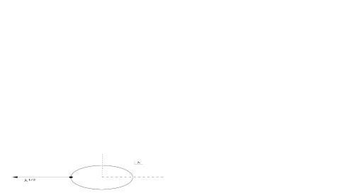
Figure 3: The complex $\lambda$-plane. The expansion of the four-point correlator around $\lambda=\infty$ is double-valued and indicates a branch cut. We represent it here from $\lambda=-1$ to the point at (minus) infinity.

The explicit background expansion of the covariantized four-graviton scattering amplitude resummed in derivatives produces the Gamma function form in (4.1). Indeed, the ratio of Gamma functions is of the form, $\alpha^{\prime}s_{\rm bdy}\rightarrow(\alpha^{\prime}/R_{AdS}^{2})~{}z_{0}^{2}~{}(k_{1}+k_{2})\cdot(k_{1}+k_{2})$,

$${\Gamma(1-\lambda^{-1/2}s)\Gamma(1-\lambda^{-1/2}t)\Gamma(1-\lambda^{-1/2}u)\over\Gamma(1+\lambda^{-1/2}s)\Gamma(1+\lambda^{-1/2}t)\Gamma(1+\lambda^{-1/2}u)}\ ,$$ (4.7)

where the invariants represent the differential operators in the $(1,2)$, $(1,3)$ and $(2,3)$ channels such that

$$s=z_{0}^{2}\bigl{(}{\partial\over\partial z_{0}}{\partial\over\partial z_{0}}+({\partial\over\partial{\vec{x}}_{1}}+{\partial\over\partial{\vec{x}}_{2}})\cdot({\partial\over\partial{\vec{x}}_{1}}+{\partial\over\partial{\vec{x}}_{2}})\bigr{)}\ ,$$ (4.8)

where the Fourier expansion would generate $(k_{1}+k_{2})^{2}$ in the boundary components from the partial derivatives. The explicit evaluation of the generating function, or one-parameter integral, for the $N_{c}\rightarrow\infty$ and finite $\lambda$ correlation function requires the Gamma function with the differential argument in (4.8)

$$\mathop{\rm lim}_{N\rightarrow\infty}\langle\prod_{j=1}^{4}T^{a_{j}b_{j}}({\vec{x}}_{j})\rangle=N^{2}\int{dz_{0}d^{d}{\vec{z}}\over z_{0}^{d+1}}~{}{1\over stu}{\Gamma(1-\lambda^{-1/2}s)\Gamma(1-\lambda^{-1/2}t)\Gamma(1-\lambda^{-1/2}u)\over\Gamma(1+\lambda^{-1/2}s)\Gamma(1+\lambda^{-1/2}t)\Gamma(1+\lambda^{-1/2}u)}$$ (4.9)

$$\times\Bigl{[}\prod_{i=1}^{4}G^{\{a_{i}b_{i}\}}{}_{\{\mu_{i}\nu_{i}\}}({\vec{x}}_{i};z_{0},{\vec{z}})\Bigr{]}\prod_{j=1}^{4}\bigl{\{}{\delta\over\delta{\hat{g}}_{\mu_{j}\nu_{j}}(z_{0},{\vec{z}})}\bigr{\}}\Bigl{[}R^{4}\Bigr{]}|_{g_{AdS_{5}\times S^{5}}}~{}\ ,$$ (4.10)

together with the propagation associated withe the graviton intermediate lines; the expression in (4.10) can be understood as an infinite expansion given in (4.6) of the $k\geq 0$ terms, but resummed. We have included only the four-point graviton scattering in (4.10), and there are further contributions from the background effects associated with the terms in (2.5) and (2.8). The integration over the ${\vec{z}}$ components in (4.10) is straightforward after Fourier transforming to momentum space. The $\lambda$ dependence is manifest in (4.10). We comment on three points regarding the integral form in (4.10).

First, because the Gamma function structure in the integrand is inverted under $\lambda^{-1/2}\rightarrow-\lambda^{-1/2}$ the one-parameter integral (in $z_{0}$) representing the infinite $N_{c}$ correlator in (4.10) satisfies the reflection property,

$$\mathop{\rm lim}_{N\rightarrow\infty}\langle\prod_{j=1}^{4}T_{a_{j}b_{j}}({\vec{x}}_{j})\rangle~{}|_{e^{i\theta}|\lambda|^{-1/2}}=\Bigl{[}\mathop{\rm lim}_{N\rightarrow\infty}\langle\prod_{j=1}^{4}T_{a_{j}b_{j}}({\vec{x}}_{j})\rangle~{}|_{e^{-i\theta}|\lambda|^{-1/2}}\Bigr{]}^{\star}\ ,$$ (4.11)

for $\theta<\pi$. The inclusion of the massless graviton exchange is one term in the series and by normalization is $\lambda$ independent in the field theory; it does not change the analysis. As a function of the complex parameter $\lambda^{-1}=e^{i\phi}|\lambda|^{-1}$, it has a branch cut in the complex $\lambda$-plane; taking $\lambda^{-1}=e^{i\phi}|\lambda|^{-1}$ and sending $\phi\rightarrow\phi+2\pi$ the Gamma functions in (4.10) get inverted. After rotating twice in the complex plane the correlation function is invariant,

$$\mathop{\rm lim}_{N\rightarrow\infty}\langle\prod_{j=1}^{4}T_{a_{j}b_{j}}({\vec{x}}_{j})\rangle~{}|_{e^{4\pi i}\lambda}=\mathop{\rm lim}_{N\rightarrow\infty}\langle\prod_{j=1}^{4}T_{a_{j}b_{j}}({\vec{x}}_{j})\rangle~{}|_{\lambda}\ .$$ (4.12)

The square root of the coupling is what is required to make the dual correlator form in (4.10) invariant after two rotations in the complex plane. In perturbation theory the correlator is termwise a function of $\lambda$ and so this monodromy structure does not appear in the perturbative series without resumming. At small $\lambda$ coupling in perturbation theory there is no phase associated with the termwise rotation under $\lambda\rightarrow e^{2\pi i}\lambda$. A square root branch cut reflecting the double cover of the $\lambda$ plane possibly exists from $\lambda=-1$ to the point at infinity, illustrated in figure 5. There is a $Z_{2}$ ambiguity in relating the dual strongly coupled limit of the ${\cal N}=4$ gauge theory with that of the IIB superstring because of the branch cut in this description. The relation (1.1) together with the non-invariance of string theory as $\alpha^{\prime}\rightarrow-\alpha$ is the origin of the ambiguity.

Second, the free-field limit of the correlation function in ${\cal N}=4$ super Yang-Mills theory is related to the Gross-Mende limit of the string scattering. The evaluation may be approximated by the application of Stirling’s formula,

$$\Gamma(z)=\sqrt{2\pi}z^{z-{1/2}}e^{-z}~{}\bigl{[}1+{\cal O}({1\over z})\bigr{]}\ ,$$ (4.13)

which might enable a comparison with the free-field theory limit obtained at $\lambda=0$.

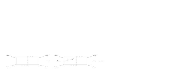
Figure 4: The unitarity properties of the correlator in the two-particle channel at finite $\lambda$ has a non-trivial structure found by summing and reexpanding the perturbative series. The string tree exchange in (4.10) generates unitarity cuts after integration over $z_{0}$, found alternatively by resumming the low-energy scattering.

Our third point refers to the unitarity structure and its comparison with the dual field theory result. As in (2.13) the holographic integral representation is found by four variations of the Einstein frame result in (4.1) together with an integration over the bulk points. The massless graviton contribution is obtained at low-energy by integrating over the supergravity modes directly in the AdS background. In the approximated form given in (4.6) the unitarity cut in the two-particle $(12)$ channel (analyzed in detail in [41]) found by

$$\mathop{\rm Im}_{s<0}~{}\langle\prod_{j=1}^{4}T_{a_{j}b_{j}}({\vec{k}}_{j})\rangle\ ,$$ (4.14)

in the regime,

$$({\vec{k}}_{1}+{\vec{k}}_{2})^{2}<0\qquad({\vec{k}}_{1}+{\vec{k}}_{4})\geq 0,\quad({\vec{k}}_{2}+{\vec{k}}_{4})^{2}\geq 0\ ,$$ (4.15)

is not clear because the four-point graphs do not individually in perturbation theory possess the poles to extract the imaginary part. However, after resumming the expansion, i.e. in the form of (4.1), the poles at arbitrary mass level (and intermediate $\lambda$ are obtained). Indeed, individually from the weak-coupling series in ${\cal N}=4$ super Yang-Mills theory there are unitarity cuts in the two-particle channel generically at every order in $\lambda$, illustrated in figure 6. They are found by integrating over $z_{0}$ and summing the series in $\alpha^{\prime}$; the poles of the gamma function in (4.1) are obtained by integrating over $z_{0}$ at fixed momenta. The integration over $z_{0}$ in (4.10) in principle extracts the unitarity cuts of the complete ${\cal N}=4$ super Yang-Mills result (expanded around $\lambda\rightarrow\infty$ as opposed to $\lambda\rightarrow 0$) [45].

5 Space-Time Structure

Here we calculate the explicit dependence of the contact diagram contributions to the stress tensor four-point function given by (2.15). This leads to expressions involving Feynman parameter integrals which give rise to power series in the cross-ratios in general. For analysing the OPE structure of these expressions we evaluate these integrals in the limit when two of the four points approach each other. In Section 5.1 we discuss the OPE of two stress tensors for a general conformal field theory in $d$ dimensions. In Section 5.2 we turn to the OPE behaviour of the four-point function arising from (2.15). In Sections 5.3 and 5.4 we analyze the triangle integrals arising in the discussion of the space-time structure for arbitrary separation of the four points. Related OPE investigations may be found in [46, 47, 48, 49].

5.1 Operator Product Expansion

For a general $d$-dimensional CFT, the stress tensor OPE contains terms of the form $(\vec{x}_{21}\equiv\vec{x}_{1}-\vec{x}_{2})$

$$T_{a_{1}b_{1}}(\vec{x}_{1})T_{a_{2}b_{2}}(\vec{x}_{2})$$ (5.1)

$$\sim \,t^{O}_{a_{1}b_{1},a_{2}b_{2}}(\vec{x}_{21})\,O_{0}(\vec{x}_{2})+t^{V}_{a_{1}b_{1},a_{2}b_{2},k}(\vec{x}_{21})V_{k}(\vec{x}_{2})+t^{T}_{a_{1}b_{1},a_{2}b_{2},kl}(\vec{x}_{21})\,T_{kl}(\vec{x}_{2})\,+\cdots\,,$$

where $O_{0}$ is a dimensionless scalar and $V_{k}$ is a conserved vector current of dimension $d-1$. The terms shown explicitly are all leading terms in the sense that the tensors $t$ are of dimension $t\sim|x_{21}|{}^{\lambda}$ which $\lambda\geq d$, such that they may potentially give rise to poles by virtue of [50]

$$\frac{1}{|\vec{x}_{12}|^{\lambda}}\sim\frac{1}{d+2n-\lambda}\frac{1}{2^{2n}n!}\frac{2\pi^{d/2}}{\Gamma(d/2+n)}\,(\partial^{2})^{n}\delta^{d}(\vec{x}_{12})\,,$$ (5.2)

where $n=0,1,2\dots$. There are leading contributions to (5.1), where ‘leading’ is used in the sense discussed above, for example scalar operators of dimension $\eta\leq d$ or from a two-form operator $F_{ab}$ of scale dimension $d-2$. For our discussion here however it is sufficient to consider the terms shown. Of course there are also non-leading terms contributing to (5.1). As discussed extensively in [51], [52] , the tensors $t$ play a crucial role in constructing conformal three-point functions. In [51] it was shown that for a $d$-dimensional CFT, the three-point function involving two stress tensors and a third operator ${\cal O}_{J}$ of arbitrary spin $J$ and dimension $\eta$ (here ${\cal O}_{J}\in\{O_{0},V_{k},T_{kl}\}$) is given to leading order by

$$\langle T_{a_{1}b_{1}}(\vec{x}_{1})T_{a_{2}b_{2}}(\vec{x}_{2})T_{a_{3}b_{3}}(\vec{x}_{3})\rangle = \frac{{\cal I}^{T}{}_{a_{2}b_{2},kl}(\vec{x}_{21}){\cal I}^{T}{}_{a_{3}b_{3},mn}(\vec{x}_{31})}{|\vec{x}_{21}|^{2d}|\vec{x}_{31}|^{2d}}t^{J}{}_{kl,mn,J}(X)\,,$$ (5.3)

where

$$X_{k}\equiv\frac{{\vec{x}}_{21}{}_{k}}{|\vec{x}_{21}|^{2}}-\frac{\vec{x}_{31}{}_{k}}{|\vec{x}_{31}|^{2}}\quad,\,{\cal I}^{T}{}_{ab,kl}(x)\equiv{\cal E}_{ab,mn}I_{mk}(x)I_{nl}(x)\,.$$ (5.4)

Here

$$I_{ab}(\vec{y})=\delta_{ab}-2{\vec{y}_{a}\vec{y}_{b}\over|\vec{y}|^{2}}$$ (5.5)

is the defining representation of the inversion and

$${\cal E}_{kl,mn}={\textstyle\frac{1}{2}}(\delta_{km}\delta_{ln}+\delta_{lm}\delta_{kn})-{\textstyle\frac{1}{d}}\delta_{km}\delta_{ln}$$ (5.6)

the projector onto traceless symmetric tensors which satisfies

$${\cal E}_{ij,kl}I_{lm}=\delta_{ik}I_{jm}+\delta_{jk}I_{im}-{1\over d}\delta_{ij}I_{km}\ .$$ (5.7)

It was shown in [51] that the form (5.3) for the conformal three-point function is unique in the sense that it is both necessary and sufficient. The tensor $t^{J}$ has to satisfy constraints arising from symmetry and stress-tensor conservation.

Let us now consider the stress tensor four-point function. When $\vec{x}_{1}\rightarrow\vec{x}_{2}$ we have ($\vec{x}_{21}\equiv\vec{x}_{2}-\vec{x}_{1}$)

$$\langle T_{a_{1}b_{1}}({\vec{x}}_{1})T_{a_{2}b_{2}}({\vec{x}}_{2})T_{a_{3}b_{3}}({\vec{x}}_{3})T_{a_{4}b_{4}}({\vec{x}}_{4})\rangle$$

$$= t^{O}_{a_{1}b_{1},a_{2}b_{2}}(\vec{x}_{21})\langle O_{0}({\vec{x}}_{2})T_{a_{3}b_{3}}({\vec{x}}_{3})T_{a_{4}b_{4}}({\vec{x}}_{4})\rangle\,$$

$$+t^{V}_{a_{1}b_{1},a_{2}b_{2},k}(\vec{x}_{21})\langle V_{k}({\vec{x}}_{2})T_{a_{3}b_{3}}({\vec{x}}_{3})T_{a_{4}b_{4}}({\vec{x}}_{4})\rangle$$

$$+\,t^{T}_{a_{1}b_{1},a_{2}b_{2},kl}(\vec{x}_{21})\langle T_{kl}({\vec{x}}_{2})T_{a_{3}b_{3}}({\vec{x}}_{3})T_{a_{4}b_{4}}({\vec{x}}_{4})\rangle+\cdots\,,$$

where the three point functions are of the form (5.3). As was shown in [51], the three point function involving the dimensionless scalar $O_{0}(\vec{x}_{2})$ is independent of $\vec{x}_{2}$ and is proportional to the two-point function

$$\langle O_{0}({\vec{x}}_{2})T_{a_{3}b_{3}}({\vec{x}}_{3})T_{a_{4}b_{4}}({\vec{x}}_{4})\rangle\propto\langle T_{a_{3}b_{3}}({\vec{x}}_{3})T_{a_{4}b_{4}}({\vec{x}}_{4})\rangle=C_{T}\,\frac{{\cal I}^{T}_{a_{3}b_{3},a_{4}b_{4}}(x_{12})}{(x_{12}{}^{2})^{d}}\,.$$ (5.9)

Similarly $t^{O}_{a_{1}b_{1}a_{2}b_{2}}(\vec{x}_{12})$ is also proportional to the two-point function,

$$t^{O}_{a_{1}b_{1}a_{2}b_{2}}(\vec{x}_{12})\propto\langle T_{a_{3}1b_{1}}({\vec{x}}_{1})T_{a_{2}b_{2}}({\vec{x}}_{2})\rangle\,,$$ (5.10)

such that the dimensionless scalar in the OPE leads to the contribution to the four-point function which factors into two two-point functions,

$$\langle T_{a_{1}b_{1}}({\vec{x}}_{1})T_{a_{2}b_{2}}({\vec{x}}_{2})T_{a_{3}b_{3}}({\vec{x}}_{3})T_{a_{4}b_{4}}({\vec{x}}_{4})\rangle_{O}\propto\langle T_{a_{1}b_{1}}({\vec{x}}_{1})T_{a_{2}b_{2}}({\vec{x}}_{2})\rangle\,\langle T_{a_{3}b_{3}}({\vec{x}}_{3})T_{a_{4}b_{4}}({\vec{x}}_{4})\rangle\,.$$ (5.11)

As discussed in [52], $\langle T_{a_{1}b_{1}}({\vec{x}}_{1})T_{a_{2}b_{2}}({\vec{x}}_{2})\rangle$ contains a pole due to (5.2). As far as $t^{T}_{a_{1}b_{1}a_{2}b_{2}kl}$ in (5.3) is concerned, it was shown in [52] that although the dimension is $t^{T}_{a_{1}b_{1}a_{2}b_{2}kl}\sim|x_{21}|{}^{-d}$, such that a pole of type (5.2) might be expected, the tensorial structure ensures that there is no such pole if energy-momentum conservation is imposed. We expect a similar result to hold for $t^{V}_{a_{1}b_{1}a_{2}b_{2}k}$.

5.2 String theory contributions to the stress tensor four-point function

We are going to show that the contribution to the stress tensor four-point function (2.15), which corresponds to contact diagrams for the graviton scattering, does not contain any leading OPE term in the sense that when $x_{1}\rightarrow x_{2}$, there is no term involving $|\vec{x}_{21}|{}^{-\lambda}$ with $\lambda\geq d$, which implies that the tensors $t^{J}$ discussed above are identically zero for this contribution. For the explicit evaluation of (2.15) we generalize techniques developed in [53]. At first we consider the case $k=0$ in (2.15), which corresponds to the well-known $R^{4}$ term, and discuss the extension to $k\neq 0$ and to the five-form terms later on.

For the $AdS_{5}$ geometry we use the conventions of [5]. We use the $AdS_{5}$ bulk-to-boundary propagator in the the Donder gauge [54], which is given by

$$G_{\mu\nu,}{}_{ab}({\vec{x}};z_{0},{\vec{z}})=\Bigl{[}(d+1){\Gamma(d-1)\over\pi^{d/2}\Gamma({d\over 2})}\Bigr{]}{z_{0}{}^{d-2}\over\left(z_{0}^{2}+|{\vec{z}}-{\vec{x}}|^{2}\right)^{d}}I_{\mu k}(z-{\vec{x}})I_{\nu l}(z-{\vec{x}}){\cal E}_{kl}{}_{ab}\ .$$ (5.12)

Our conventions for the connection and for the covariant derivatives are

$$\Gamma_{\mu\nu}{}^{\kappa}=-{1\over z_{0}}\Bigl{[}\eta_{\mu}^{0}\eta^{\kappa}_{\nu}+\eta_{\nu}^{0}\eta^{\kappa}_{\mu}-\eta^{0\kappa}\eta_{\mu\nu}\Bigr{]}\ ,$$ (5.13)

$$\nabla_{\mu}V_{\nu}=\partial_{\mu}V_{\nu}-\Gamma_{\mu\nu}{}^{\kappa}V_{\kappa}\ ,$$ (5.14)

where for the AdS metric we have $g_{\mu\nu}={1\over z_{0}^{2}}\eta_{\mu\nu}$. For evaluating the vertex given by (2.15) we make use of the fact that for the metric fluctuations around the background we have

$$\delta R_{\mu\sigma\rho\nu}=\nabla_{[\mu}\nabla_{[\nu}\delta g_{\rho]\sigma]}\,,$$ (5.15)

where the antisymmetrization is in pairs $[\mu,\sigma]$ and $[\nu,\rho]$. We find that

$$\nabla_{[\mu}^{z}\nabla_{[\nu}^{z}G_{\rho]\sigma];ab}(z,{\vec{x}}) = \Bigl{[}{\Gamma(d+2)\over\pi^{d/2}\Gamma({d\over 2})}\Bigr{]}\,{z_{0}^{d-4}\over(z-{\vec{x}})^{2d}}$$ (5.16)

$$\times\Bigl{[}I_{0[\mu}I_{\sigma]k}I_{0[{\nu}}I_{{\rho}]l}{\cal E}_{kl,ab}-{\frac{1}{d}}\eta_{[\mu[\nu}I_{\sigma]k}I_{\rho]l}{\cal E}_{kl,ab}\Bigr{]}(z-{\vec{x}})\,,$$

the form of which is of particular importance for the evaluation of the four-point function. This result is very similar to a result of [5] for the bulk-to-boundary gauge field propagator $G^{G}$ for which

$$G^{G}_{\mu i}(z,\vec{x}) = C^{d}\frac{z_{0}^{d-2}}{(z-\vec{x})^{2(d-1)}}\,I_{\mu i}(z-\vec{x})\,,$$

$$\partial_{[\mu}G^{G}_{\nu]i}(z,\vec{x}) = (d-2)C^{d}\frac{z_{0}^{d-3}}{(z-\vec{x})^{2(d-1)}}\,I_{0[\mu}(z-\vec{x})I_{\nu]i}(z-\vec{x})\,,$$ (5.17)

where $\partial_{[\mu}G^{G}_{\nu]i}$ is gauge invariant. We note that if the second term in (5.16) had the factor $(d-1)^{-1}$ instead of $d^{-1}$, $\nabla\nabla G$ would have the index symmetry of the Weyl tensor in five dimensions when $d=4$. However since the factor is $d^{-1}$ this seems not to be the case. Although the vertex (2.15) has Weyl index symmetry in $d=10$, this structure seems to be lost when just considering the AdS part of the compactification $AdS_{5}\times S_{5}$. See also [55].

With these ingredients the stress tensor four-point function defined in (2.15) is given by

$$T_{a_{1}b_{1}a_{2}b_{2}a_{3}b_{3}a_{4}b_{4}}(\vec{x}_{1},\vec{x}_{2},\vec{x}_{3},\vec{x}_{4})$$

$$= \int\!\!\frac{d^{d+1}z}{z_{0}^{d+1}}t^{8\mu_{1}\sigma_{1}\cdots\mu_{4}\sigma_{4}}t^{8\nu_{1}\rho_{1}\cdots\nu_{4}\rho_{4}}\nabla_{[\rho_{1}}\nabla_{[\sigma_{1}}G_{\mu_{1}]\nu_{1}],a_{1}b_{1}}(z-\vec{x}_{1})\cdots\nabla_{[\rho_{4}}\nabla_{[\sigma_{4}}G_{\mu_{4}]\nu_{4}],a_{4}b_{4}}(z-\vec{x}_{4})$$

$$= \int\!\!\frac{d^{d+1}z}{z_{0}^{d+1}}t^{8}_{\mu_{1}\sigma_{1}\cdots\mu_{4}\sigma_{4}}t^{8}_{\nu_{1}\rho_{1}\cdots\nu_{4}\rho_{4}}{\cal E}_{a_{1}b_{1},k_{1}l_{1}}\cdots{\cal E}_{a_{4}b_{4},k_{4}l_{4}}$$

$$\;\qquad\quad\times\,{\cal I}^{R}_{0\mu_{1}\sigma_{1}k_{1}l_{1}\rho_{1}\nu_{1}0}(z-\vec{x}_{1}){\cal I}^{R}_{0\mu_{2}\sigma_{2}k_{1}l_{2}\rho_{2}\nu_{2}0}(z-\vec{x}_{2})$$

$$\;\qquad\quad\times\,{\cal I}^{R}_{0\mu_{3}\sigma_{3}k_{1}l_{3}\rho_{3}\nu_{3}0}(z-\vec{x}_{3}){\cal I}^{R}_{0\mu_{4}\sigma_{4}k_{1}l_{4}\rho_{4}\nu_{4}0}(z-\vec{x}_{4})\,,$$

where

$${\cal I}^{R}_{0\mu\sigma kl\rho\nu 0}(z-\vec{x}) = \left[\frac{\Gamma(d+2)}{\pi^{d/2}\Gamma(d/2)}\right]\frac{z_{0}^{d}}{(z-\vec{x})^{2d}}\,(I_{0[\mu}I_{\sigma]k}I_{l[\rho}I_{\nu]0}-{\textstyle\frac{1}{d}}\delta_{[\mu[\nu}I_{\rho]k}I_{\sigma]l})(z-\vec{x})\,.$$ (5.19)

The overall factor of $z_{0}^{16}$ compensates for the lowering of sixteen indices. For reference the explicit expression for the $t^{8}$ tensor is given in the Appendix.

We perform an inversion in $\vec{x}_{1}$ according to the method of [5] and define

$$\vec{x}^{\prime}_{21\,k}=\frac{\vec{x}_{21\,k}}{|\vec{x}_{21}|^{2}}\,.$$ (5.20)

This gives for the four-point correlation function as given by (5.2)

$$T_{a_{1}b_{1}a_{2}b_{2}a_{3}b_{3}a_{4}b_{4}}(\vec{x}_{1},\vec{x}_{2},\vec{x}_{3},\vec{x}_{4})$$ (5.21)

$$= \frac{{\cal I}^{T}_{a_{2}b_{2},k_{2}l_{2}}(\vec{x}_{21}){\cal I}^{T}_{a_{3}b_{3},k_{3}l_{3}}(\vec{x}_{31}){\cal I}^{T}_{a_{4}b_{4},k_{4}l_{4}}(\vec{x}_{41}){\cal E}_{a_{1}b_{1}k_{1}l_{1}}}{|\vec{x}_{21}|^{2d}|\vec{x}_{31}|^{2d}|\vec{x}_{41}|^{2d}}t^{TTTT}_{k_{1}l_{1}k_{2}l_{2}k_{3}l_{3}k_{4}l_{4}}(\vec{x}^{\prime}_{23},\vec{x}^{\prime}_{24})\,,$$

where

$$t^{TTTT}_{k_{1}l_{1}k_{2}l_{2}k_{3}l_{3}k_{4}l_{4}}(\vec{x}^{\prime}_{23},\vec{x}^{\prime}_{24})$$ (5.22)

$$=\int\!\!\frac{d^{d+1}z^{\prime}}{z^{\prime}_{0}{}^{d+1}}t^{8}_{\mu_{1}\sigma_{1}\cdots\mu_{4}\sigma_{4}}t^{8}_{\nu_{1}\rho_{1}\cdots\nu_{4}\rho_{4}}(\delta_{0[\mu_{1}}\delta_{\sigma_{1}]k_{1}}\delta_{l_{1}[\rho_{1}}\delta_{\nu_{1}]0}-{\textstyle\frac{1}{d}}\delta_{\mu_{1}[\nu_{1}}\delta_{\rho_{1}]k_{1}}\delta_{\sigma_{1}]l_{1}})$$

$$\;\;\times{\cal I}^{R}_{0\mu_{2}\sigma_{2}k_{2}l_{2}\rho_{2}\nu_{2}0}(z^{\prime}-\vec{x}^{\prime}_{21}){\cal I}^{R}_{0\mu_{3}\sigma_{3}k_{3}l_{3}\rho_{3}\nu_{3}0}(z^{\prime}-\vec{x}^{\prime}_{31}){\cal I}^{R}_{0\mu_{4}\sigma_{4}k_{4}l_{4}\rho_{4}\nu_{4}0}(z^{\prime}-\vec{x}^{\prime}_{41})\,.$$

${\cal I}^{T}$ is given by (5.4). In defining $t^{TTTT}$ we have used the fact that the integral in (5.22) depends only on the differences

$$\vec{x}^{\prime}_{23\,k}=\frac{\vec{x}_{21\,k}}{|\vec{x}_{21}|^{2}}-\frac{\vec{x}_{31\,k}}{|\vec{x}_{31}|^{2}}\,,\quad\vec{x}^{\prime}_{24\,k}=\frac{\vec{x}_{21\,k}}{|\vec{x}_{21}|^{2}}-\frac{\vec{x}_{41\,k}}{|\vec{x}_{41}|^{2}}\,.$$ (5.23)

Note that these variables are of the same form as the variable $X$ in (5.4). The expression (5.21) is very reminiscent of the general construction procedure for conformal three-point functions of [51, 52] as described in 5.1, and gives some indication how this procedure may be generalized to four-point functions.

The next step is the evaluation of the integral in (5.22). Since this is a tedious task we just outline the calculation here and proceed to the determination of the leading terms when $\vec{x}_{1}\rightarrow\vec{x}_{2}$. In the general case the evaluation of the integral necessitates the extraction of derivatives with respect to the $\vec{x}^{\prime}_{m}$ such as to obtain a collection of scalar integrals. In order to achieve this, we decompose the sum over indices in (5.22) by writing $\mu\,\hat{=}\,(0,m)$, where $0$ stands for the bulk coordinate and the Latin indices for the coordinates parallel to the boundary. We demonstrate this procedure using the simple example of two antisymmetric tensors $M$ and $N$:

$$M_{\mu\nu}N_{\mu\nu}=2M_{0n}N_{0n}+M_{mn}N_{mn}.$$ (5.24)

Some terms in the sum in (5.22) obtained this way vanish due to

$$t^{8}_{0kijmnpq}=0\quad t^{8}_{0k0j0npq}=0.$$ (5.25)

From the expressions

$${\cal I}^{R}_{0msklrn0}\,,{\cal I}^{R}_{00sklr00}\,,{\cal I}^{R}_{0msklr00}$$ (5.26)

the necessary derivatives with respect to $\vec{x}$ may be extracted using the algebraic computing program FORM. The results are given in the Appendix.

The procedure outlined here gives a sum of scalar integrals of the type

$${\cal I}=\int\!\!\frac{d^{d+1}z^{\prime}}{z^{\prime}_{0}{}^{d+1}}\,\frac{z_{0}^{\sum\limits_{i=1}^{4}\Delta_{i}}}{(z^{\prime}-\vec{x}^{\prime}_{21})^{2\Delta_{2}}(z^{\prime}-\vec{x}^{\prime}_{31})^{2\Delta_{3}}(z^{\prime}-\vec{x}^{\prime}_{41})^{2\Delta_{4}}}\,,$$ (5.27)

with a collection of derivatives acting on them. There are at most four derivatives for every $x$. The tensor structure is completed by a number of Kronecker $\delta$’s. The integral (5.27) may be evaluated using Feynman parameter methods which give

$${\cal I} = \pi^{d/2}\frac{\Gamma[(\sum\limits_{i=1}^{4}\Delta_{i}-d)/2]\Gamma[{\textstyle\frac{1}{2}}(\Delta_{2}+\Delta_{3}+\Delta_{4}-\Delta_{1})]}{2\Gamma[\Delta_{2}]\Gamma[\Delta_{3}]\Gamma[\Delta_{4}]}$$

$$\times\,\int\!\!\ \prod_{j=2}^{4}d\alpha_{j}~{}\delta(1-\sum\limits_{i}\alpha_{i})~{}\frac{{\alpha_{j}^{\Delta_{j}-1}}}{(\alpha_{2}\alpha_{3}|\vec{x}^{\prime}_{23}|^{2}+\alpha_{2}\alpha_{4}|\vec{x}^{\prime}_{24}|^{2}+\alpha_{3}\alpha_{4}|\vec{x}^{\prime}_{34}|^{2})^{{\textstyle\frac{1}{2}}(\Delta_{2}+\Delta_{3}+\Delta_{4}-\Delta_{1})}}\,,$$

with $\vec{x}^{\prime}_{23},\vec{x}^{\prime}_{24}$ given by (5.23) and $\vec{x}^{\prime}_{34}=\vec{x}^{\prime}_{24}-\vec{x}^{\prime}_{23}$. By a standard change of variables we obtain

$${\cal I} = \pi^{d/2}\frac{\Gamma[(\sum\limits_{i=1}^{4}\Delta_{i}-d)/2]\Gamma[{\textstyle\frac{1}{2}}(\Delta_{2}+\Delta_{3}+\Delta_{4}-\Delta_{1})]}{2\Gamma[\Delta_{2}]\Gamma[\Delta_{3}]\Gamma[\Delta_{4}]}$$

$$\times\,\int\!\!d{\beta_{2}}d{\beta_{3}}\frac{\beta_{2}^{\Delta_{2}-1}\beta_{3}^{\Delta_{3}-1}}{(1+\beta_{2}+\beta_{3})^{\Delta_{1}}}\,\frac{1}{|\vec{x}^{\prime}_{23}|^{{\textstyle\frac{1}{2}}(\Delta_{2}+\Delta_{3}+\Delta_{4}-\Delta_{1})}(\beta_{2}\beta_{3}+\xi\beta_{3}+\eta\beta_{2})^{{\textstyle\frac{1}{2}}(\Delta_{2}+\Delta_{3}+\Delta_{4}-\Delta_{1})}}\ ,$$

where we have introduced the conformally invariant cross-ratios,

$$\eta=\frac{|\vec{x}^{\prime}_{24}|^{2}}{|\vec{x}^{\prime}_{23}|^{2}}=\frac{|\vec{x}_{24}|^{2}|\vec{x}_{31}|^{2}}{|\vec{x}_{23}|^{2}|\vec{x}_{41}|^{2}}\,,\quad\xi=\frac{|\vec{x}^{\prime}_{34}|^{2}}{|\vec{x}^{\prime}_{23}|^{2}}=\frac{|\vec{x}_{34}|^{2}|\vec{x}_{21}|^{2}}{|\vec{x}_{23}|^{2}|\vec{x}_{41}|^{2}}\,.$$ (5.30)

In general this integral gives a power series involving a generalized hypergeometric function. However for our purpose it is sufficient to consider the case when $|\vec{x}_{12}|\rightarrow 0$ in which

$$\eta\rightarrow 1\,,\quad\xi\rightarrow|\vec{x}_{21}|^{2}\frac{|\vec{x}_{34}|^{2}}{|\vec{x}_{32}|^{2}|\vec{x}_{34}|^{2}}\,=|\vec{x}_{21}|^{2}|\vec{x}^{\prime}_{34}|^{2}\,,$$ (5.31)

and $|\vec{x}^{\prime}_{23}|^{-\Delta}\simeq|\vec{x}_{21}|^{\Delta}$. Although the form in (5.2) is sufficient to extract the leading behavior, we perform a further transformation as in [21] to simplify the analysis,

$$\beta_{2}\rightarrow\beta_{2}^{\prime}=\frac{\beta_{2}}{\beta_{3}}(1+\beta_{3})\,,$$ (5.32)

which gives, omitting the overall prefactor,

$${\cal I}^{\prime} = \int\!\!d\beta_{2}^{\prime}d\beta_{3}\,\frac{\beta_{3}^{{\textstyle\frac{1}{2}}(\Delta_{1}+\Delta_{2}+\Delta_{3}-\Delta_{4})}}{(1+\beta_{3})^{\Delta_{2}}(1+\beta_{3}+\beta_{2}^{\prime}\frac{\beta_{3}}{1+\beta_{3}})^{\Delta_{1}}}\,\frac{\beta^{\prime}_{2}{}^{\Delta_{2}-1}}{(\beta^{\prime}_{2}+\xi)^{{\textstyle\frac{1}{2}}(\Delta_{2}+\Delta_{3}+\Delta_{4}-\Delta_{1})}}\,.$$ (5.33)

For $\Delta_{2}+\Delta_{1}>\Delta_{3}+\Delta_{4}$ we see that when $\xi\rightarrow 0$ the dominant contribution to the $\beta_{2}^{\prime}$ integral comes from the region where $\beta^{\prime}_{2}\simeq 0$. In this region the second tern in the denominator of (5.33) is independent of $\beta^{\prime}_{2}$ and the integral factors to give

$${\cal I} \sim K\,|\vec{x}_{21}|^{\Delta_{2}+\Delta_{3}+\Delta_{4}-\Delta_{1}}\,\xi^{{\textstyle\frac{1}{2}}(\Delta_{2}+\Delta_{1}-\Delta_{3}-\Delta_{4})}\,=\,K|\vec{x}_{21}|^{2\Delta_{2}}|\vec{x}^{\prime}_{34}|^{(\Delta_{2}+\Delta_{1}-\Delta_{3}-\Delta_{4})}\,,$$ (5.34)

$$K = \frac{1}{\Gamma[\Delta_{1}+\Delta_{2}]\Gamma[\Delta_{3}]\Gamma[\Delta_{4}]}\,\Big{\{}\Gamma[(\sum\Delta_{i}-d)/2]\Gamma[(\Delta_{3}+\Delta_{4}-\Delta_{2}-\Delta_{1})/2]$$

$$\hskip-2.84544pt\times\,\Gamma[(\Delta_{3}+\Delta_{4}-\Delta_{2}-\Delta_{1})/2]\Gamma[(\Delta_{1}+\Delta_{2}+\Delta_{3}-\Delta_{4})/2]\Gamma[(\Delta_{1}+\Delta_{2}+\Delta_{4}-\Delta_{3})/2]\Big{\}}\,.$$

For $\Delta_{2}+\Delta_{1}=\Delta_{3}+\Delta_{4}$ we perform the $\beta^{\prime}_{2}$ integral explicitly which leads to a hypergeometric function whose leading term involves ${\rm ln}\xi$. In this case we have

$${\cal I}\sim\frac{\pi^{d}}{2}\frac{\Gamma[(\sum\Delta_{i}-d)/2]}{\Gamma[\Delta_{1}+\Delta_{2}]}\,|\vec{x}_{21}|^{2\Delta_{2}}\,({\rm const.}-{\rm ln}\xi)\,.$$ (5.35)

With the help of these general results we may determine the leading behaviour of (5.22). As an example for a term present in (5.22) we consider

$$\delta_{a_{1}b_{1}}\delta_{a_{2}b_{2}}\delta_{a_{3}b_{3}}\delta_{a_{4}b_{4}}P_{0}\equiv\delta_{a_{1}b_{1}}\delta_{a_{2}b_{2}}\delta_{a_{3}b_{3}}\delta_{a_{4}b_{4}}\int\!\!\frac{d^{d+1}z^{\prime}}{z^{\prime}_{0}{}^{d+1}}\;\frac{z^{\prime}_{0}{}^{d}}{(z^{\prime}-\vec{x}^{\prime}_{21})^{2d}(z^{\prime}-\vec{x}^{\prime}_{31})^{2d}(z^{\prime}-\vec{x}^{\prime}_{41})^{2d}}\,$$ (5.36)

Here no extraction of derivatives is necessary since the tensor structure is entirely given by Kronecker deltas. Using the results for Feynman integrals described above, in particular (5.34), we find for $\vec{x}_{1}\rightarrow\vec{x}_{2}$:

$$P_{0}\propto|\vec{x}_{21}|^{2d}\,({\rm const.}-\ln\xi)\quad.$$ (5.37)

Together with the factor of ${\cal I}^{T}/x_{21}^{2d}$ present in (5.22) we see that in the limit $\vec{x}_{1}\rightarrow\vec{x}_{2}$ the contribution (5.36) depends only on dimensionless combinations of $\vec{x}_{21}$ such as $\vec{x}_{21\,a}\vec{x}_{21\,b}/x_{21}{}^{2}$ and $\ln\xi$. (5.36) does not give rise to any poles for which according to (5.2) a dependence of the form $|\vec{x}_{21}|^{-\lambda}$ with $\lambda\geq d$ is necessary.

By simple power-counting we may determine the $|\vec{x}_{21}|$ dependence of the terms in (5.22) involving derivatives. In extracting the derivatives a dimensional regulation in $d$ is used to ensure finite scalar integrals at every step of the calculation. However after taking the derivatives again after evaluating the integrals, all expressions are finite such that the regulator may be taken to zero.

By inspection of the expressions for the ${\cal I}^{R}$ listed in the appendix we see that the derivative terms are of the general form

$$P_{\partial} = \delta\cdots\delta\,\partial^{x^{\prime}_{21}}\cdots\partial^{x^{\prime}_{21}}\,\partial^{x^{\prime}_{31}}\cdots\partial^{x^{\prime}_{31}}\,\partial^{x^{\prime}_{41}}\,\cdots\partial^{x^{\prime}_{41}}\;\;$$ (5.38)

$$\hskip 2.84544pt\times\,\int\!\!\frac{d^{d+1}z^{\prime}}{z_{0}^{d+1}}\,\frac{z_{0}^{\prime}{}^{4d+2\sum a_{i}+b}}{(z^{\prime}-\vec{x}_{21})^{2(d-n_{2}/2+a_{2})}(z^{\prime}-\vec{x}_{31})^{2(d-n_{3}/2+a_{3}}(z^{\prime}-\vec{x}_{41})^{2(d-n_{4}/2+a_{4})}}\,,$$

where the tensor structure ($\delta\cdots\delta)$ in (5.38) is determined by a combination of Kronecker deltas and derivatives. Furthermore defining $q_{i}$ to be the total number of derivatives extracted with respect to the variable $x^{\prime}_{i1}$, we have for the numbers $n_{2},n_{3},n_{4}$ in (5.38)

$$q_{i}~{}\,{\rm even}\, : n_{i}\equiv q_{i}$$

$$q_{i}~{}\,{\rm odd}\, : n_{i}\equiv q_{i}+1\,.$$

The $a_{i}$ are integers for which $a_{i}\geq 0$. $b$ is an integer for which $2\geq b\geq 0$, which is non-zero if an odd number of derivatives is extracted for any of the three variables ${\vec{x}}^{\prime}_{21},{\vec{x}}^{\prime}_{31},{\vec{x}}^{\prime}_{41}$. For the discussion here we note that (5.38) may be written as a Feynman parameter integral of the form (5.2). These integrals are evaluated explicitly in Section 5.3.

We now consider the expression we obtain when consecutively evaluating the derivatives explicitly when acting on the Feynman parameter representation (5.2) and (5.38). A given derivative $\partial_{p}^{x^{\prime}_{ij}}$ may act on the denominator of the Feynman parameter integral or on factors $x^{\prime}_{ij}$ ($i,j\in\{2,3,4\}$) in the numerator created by the action of derivatives evaluated before $\partial_{p}^{x^{\prime}_{ij}}$.

For determining the scaling behaviour of the $\vec{x}_{12}$ dependence it is convenient to define the following integers:

$$n_{ij}^{(i,D)} : {\rm number\,of\,derivatives\,with\,respect\,to}\,x^{\prime}_{i1}\,{\rm acting\,on}\,x^{\prime}_{ij}\,{\rm in\,the\,denominator}$$

$${\rm\,of\,the\,Feynman\,parameter\,integral}$$

$$n_{ij}^{(i,N)} : {\rm number\,of\,derivatives\,with\,respect\,to}\,x^{\prime}_{i1}\,{\rm acting\,on}\,x^{\prime}_{ij}\,{\rm in\,the\,numerator}$$

$$N_{N}^{(2)} \equiv n_{23}^{(2,N)}+n_{24}^{(2,N)}+n_{23}^{(3,N)}+n_{24}^{(4,N)}\,,$$

$$N_{D}^{(2)} \equiv n_{23}^{(2,D)}+n_{24}^{(2,D)}+n_{23}^{(3,D)}+n_{24}^{(4,D)}.$$

We have

$$n_{2} = n_{23}^{(2,N)}+n_{2,4}^{(2,N)}+n_{23}^{(2,D)}+n_{24}^{(2,D)}\,\qquad{\rm for}\,q_{2}~{}\,{\rm even}\,,$$

$$n_{2} = n_{23}^{(2,N)}+n_{2,4}^{(2,N)}+n_{23}^{(2,D)}+n_{24}^{(2,D)}+1\,\quad{\rm for}\,q_{2}~{}\,{\rm odd}\,.$$

With these definitions we obtain

$$P_{\partial} = (x^{\prime}_{23,l_{2}}\cdots x^{\prime}_{34,l_{(D-N)}})(\delta\cdots\delta)\int\,\!\!\ \prod_{j=2}^{4}d\alpha_{j}~{}\delta(1-\sum\limits_{i}\alpha_{i})~{}$$ (5.40)

$$\times\frac{{\alpha_{j}^{\Delta_{j}-1}}}{(\alpha_{2}\alpha_{3}|\vec{x}^{\prime}_{23}|^{2}+\alpha_{2}\alpha_{4}|\vec{x}^{\prime}_{24}|^{2}+\alpha_{3}\alpha_{4}|\vec{x}^{\prime}_{34}|^{2})^{{\textstyle\frac{1}{2}}(\Delta_{2}+\Delta_{3}+\Delta_{4}-\Delta_{1})}}\,.$$

where

$$\Delta_{2}=d-n_{2}/2+N_{D}^{(2)}+a_{2}\,,\quad\Delta_{1}=d+\sum n_{i}+\sum a_{i}+b.$$ (5.41)

$\Delta_{3},\Delta_{4}$ are given by expressions similar to $\Delta_{2}$. We always have $\Delta_{1}+\Delta_{2}\geq\Delta_{3}+\Delta_{4}$. The first factor in (5.40) is a tensor product of vectors of which $N_{D}^{(2)}-N_{N}^{(2)}$ contain $\vec{x}^{\prime}_{21,l}$. In the limit $\vec{x}_{1}\to\vec{x}_{2}$ we calculate the integral using (5.34) or (5.37) to obtain

$$P_{\partial}\propto\left(\frac{\vec{x}_{21,l_{1}}}{|\vec{x}_{21}|^{2}}\cdots\frac{\vec{x}_{21,l_{(D-N)}}}{|\vec{x}_{21}|^{2}}\right)\,|\vec{x}_{21}|^{2\Delta_{2}}\,({\rm const.}-\ln\xi)\,t(\vec{x}^{\prime}_{34})\quad.$$ (5.42)

Here $\vec{x}^{\prime}_{34}$ is now independent of $\vec{x}_{1}$,

$$\vec{x}^{\prime}_{34,l}=\frac{\vec{x}_{32,l}}{|\vec{x}_{32}|^{2}}-\frac{\vec{x}_{42,l}}{|\vec{x}_{42}|^{2}}\quad.$$ (5.43)

$t$ is a tensor which is of a similar structure as the tensors $t$ in (5.3). In (5.42) there are $N_{D}^{(2)}-N_{N}^{(2)}$ factors of $\vec{x}_{21}/|\vec{x}_{21}|^{2}$. Remembering the factor ${\cal I}^{T}/|\vec{x}_{21}|^{2d}$ in (5.22) we see that all the terms contributing to (5.22) depend at most on dimensionless combinations of $\vec{x}_{21}$ if

$$2\Delta_{2}-N_{D}^{(2)}+N_{N}^{(2)}\geq 2d\quad,$$ (5.44)

which using the definitions of the integers defined in the table above (LABEL:n2) as well as (5.41) is equivalent to

$$2a_{2}+n_{24}^{(4,D)}+n_{23}^{(3,D)}+n_{24}^{(4,N)}+n_{23}^{(3,N)}\geq 0\,.$$ (5.45)

Since by definition all the integers in this condition are non-negative, this condition is always satisfied. Therefore we have proved that the contribution to the stress-tensor four-point function given by (5.22) contributes only non-leading terms involving operators of dimension $\eta\geq 2d$ to the stress-tensor OPE.

It is straightforward to see that our argument extends also to contributions with $k\neq 0$ in (2.15). Any additional $\Box^{z}=g^{\mu\nu}\nabla^{z}_{\mu}\nabla^{z}_{\nu}$ increases $N_{D}^{(2)}$ by $2$ at most, but increases $\Delta_{2}$ by the same amount at the same time such that (5.44) is not modified. Moreover the general terms in the string scattering elements, including those involving the background values of the five-form field strength in (2.5), are of the form $\Box^{k}R^{4}$, and in a similar way these terms do not contribute any leading terms to the OPE through the holographic scattering.

Finally we note that the absence of leading terms in the OPE implies that the contributions to the stress-tensor four-point function discussed here are not linked to the stress-tensor two- and three-point function by any Ward identity, which is consistent with the non-renormalization properties of the two- and three-point functions. In fact, the diffeomorphism and Weyl symmetry Ward identities expressing conservation and tracelessness of the stress tensor are of the form

$$\partial^{\vec{x}_{1}}_{a_{1}}\langle T_{a_{1}b_{1}}(\vec{x}_{1})T_{a_{2}b_{2}}(\vec{x}_{2})T_{a_{3}b_{3}}(\vec{x}_{3})T_{a_{4}b_{4}}(\vec{x}_{4})\rangle = \partial_{b_{1}}\delta^{(d)}(\vec{x}_{12})\langle T_{a_{2}b_{2}}(\vec{x}_{2})T_{a_{3}b_{3}}(\vec{x}_{3})T_{a_{4}b_{4}}(\vec{x}_{4})\rangle+\dots\,,$$

$$\langle T_{a_{1}a_{1}}(\vec{x}_{1})T_{a_{2}b_{2}}(\vec{x}_{2})T_{a_{3}b_{3}}(\vec{x}_{3})T_{a_{4}b_{4}}(\vec{x}_{4})\rangle = \delta^{(d)}(\vec{x}_{12})\langle T_{a_{2}b_{2}}(\vec{x}_{2})T_{a_{3}b_{3}}(\vec{x}_{3})T_{a_{4}b_{4}}(\vec{x}_{4})\rangle+\dots\,,$$ (5.46)

where the dots denote permutations of $(2\leftrightarrow 3\leftrightarrow 4)$ and terms involving two-point functions. According to (5.2), the necessary delta distributions on the right hand side of the Ward identity are generated by those terms on the left hand side which in the limit $\vec{x}_{1}\rightarrow\vec{x}_{2}$ involve $|\vec{x}_{21}|^{-\lambda}$ with $\lambda\geq d$, and similarly for $\vec{x}_{3},\vec{x}_{4}$. As we have shown above, the four-point function contributions discussed here do not involve such terms.

However we expect the stress-tensor four-point function contribution corresponding to exchange diagrams in the supergravity approximation to contain such leading terms, such that the Ward identities above are satisfied by the full stress-tensor four-point function obtained from the AdS/CFT correspondence. Moreover we expect massless supergravity exchange contributions to contain terms which factor into two-point functions (at leading order in $\lambda$ large).

5.3 Triangle diagram structure

In this section we give the form of all of the triangle integrals necessary to reproduce the contributions to the four-point correlation function at intermediate values of the coupling within our approach, except for the non-analytic terms which are not considered here. The form of the integral in (5.27) is related to a triple off-shell triangle integral with massless internal lines. The $d$ dimensional version of which has been evaluated in terms of Appel functions in [56, 57]. We give the form here, together with the parameters necessary to map between the two expressions.

The off-shell triangle described by

$$I[p_{1},p_{2},p_{3}]=\int{d^{d}l\over(2\pi)^{d}}~{}{1\over l^{2d_{1}}(l-p_{1})^{2d_{2}}(l-p_{1}-p_{3})^{2d_{3}}}$$ (5.47)

is related to the integral in (5.27) by the redefinition of the variables,

$$p_{1}={\vec{x}}_{32}\qquad p_{3}={\vec{x}}_{24}\ ,$$ (5.48)

and in (5.40) with

$$Q_{1}^{2}=|{\vec{x}}_{23}|^{2}\ ,\,Q_{2}^{2}=|{\vec{x}}_{24}|^{2}\ ,\,Q_{3}^{2}=|{\vec{x}}_{34}|^{2}\ ,$$ (5.49)

together with the identification of dimension $d$ and powers $d_{i}$

$$d=\sum_{j=1}^{4}\Delta_{j},\qquad d_{1}=\Delta_{2},\quad d_{2}=\Delta_{3},\quad d_{3}=\Delta_{4}\ ,$$ (5.50)

in addition to a normalization factor found after comparing the two integrals in a Schwinger proper time form. In comparing the integral forms we appeal directly to the latter form in (5.40) and refer the reader to [56, 57] for the derivation.

The result for the integral in (5.27) in terms of the two independent conformal invariant cross-ratios in (5.30) (where $\eta=Q^{2}_{2}/Q_{1}^{2}$ and $\xi=Q_{3}^{2}/Q_{1}^{2}$) is,

$$I_{\Delta_{j}}(\eta,\xi)=\sum_{j=1}^{4}A^{(j)}_{\Delta_{j}}(\eta,\xi)\ ,$$ (5.51)

with

$$\hskip-14.22636ptA^{(1)}_{\Delta_{j}}(\eta,\xi)=(-1)^{d/2}\Bigl{(}{\vec{x}}_{23}^{2}\Bigr{)}^{{d\over 2}-\Delta_{2}-\Delta_{3}-\Delta_{4}}{\Gamma\left({d\over 2}-\Delta_{2}-\Delta_{3}\right)\Gamma\left({d\over 2}-\Delta_{2}-\Delta_{4}\right)\Gamma\left(\Delta_{2}+\Delta_{3}-{d\over 2}\right)\over\Gamma\left(\Delta_{3}\right)\Gamma\left(\Delta_{4}\right)\Gamma\left(d-\Delta_{2}-\Delta_{3}\right)}$$

$$\times F_{4}\Bigl{(}\Delta_{2},\Delta_{2}+\Delta_{3}-{d\over 2},1+\Delta_{2}+\Delta_{4}-{d\over 2},1+\Delta_{2}+\Delta_{3}-{d\over 2};\eta,\xi\Bigr{)}\ ,$$ (5.52)

$$\hskip-14.22636ptA^{(2)}_{\Delta_{j}}(\eta,\xi)=(-1)^{d/2}\Bigl{(}{\vec{x}}_{23}^{2}\Bigr{)}^{-\Delta_{3}}\Bigl{(}{\vec{x}}_{24}^{2}\Bigr{)}^{{d\over 2}-\Delta_{2}-\Delta_{4}}{\Gamma\left({d\over 2}-\Delta_{2}-\Delta_{3}\right)\Gamma\left(\Delta_{2}+\Delta_{4}-{d\over 2}\right)\Gamma\left({d\over 2}-\Delta_{4}\right)\over\Gamma(\Delta_{2})\Gamma\left(\Delta_{4}\right)\Gamma\left(d-\Delta_{2}-\Delta_{3}\right)}$$

$$\times F_{4}\Bigl{(}\Delta_{3},{d\over 2}-\Delta_{4},1+{d\over 2}-\Delta_{2}-\Delta_{4},1+\Delta_{2}+\Delta_{3}-{d\over 2};\eta,\xi\Bigr{)}\ ,$$ (5.53)

$$\hskip-14.22636ptA^{(3)}_{\Delta_{j}}(\eta,\xi)=(-1)^{d/2}\Bigl{(}{\vec{x}}_{23}^{2}\Bigr{)}^{-\Delta_{4}}\Bigl{(}{\vec{x}}_{24}^{2}\Bigr{)}^{{d\over 2}-\Delta_{2}-\Delta_{3}}{\Gamma\left({d\over 2}-\Delta_{2}-\Delta_{4}\right)\Gamma\left(\Delta_{2}+\Delta_{3}-{d\over 2}\right)\Gamma\left({d\over 2}-\Delta_{3}\right)\over\Gamma\left(\Delta_{2}\right)\Gamma\left(\Delta_{3}\right)\Gamma\left(d-\Delta_{2}-\Delta_{3}\right)}$$

$$\times F_{4}\Bigl{(}\Delta_{4},{d\over 2}-\Delta_{3},1+\Delta_{2}+\Delta_{4}-{d\over 2},1+{d\over 2}-\Delta_{2}-\Delta_{3};\eta,\xi\Bigr{)}\ ,$$ (5.54)

and,

$$\hskip-56.9055ptA^{(4)}_{\Delta_{j}}(\eta,\xi)=(-1)^{d/2}\Bigl{(}{\vec{x}}_{23}^{2}\Bigr{)}^{\Delta_{2}-{d\over 2}}\Bigl{(}{\vec{x}}_{24}^{2}\Bigr{)}^{{d\over 2}-\Delta_{2}-\Delta_{4}}\Bigl{(}{\vec{x}}_{34}^{2}\Bigr{)}^{{d\over 2}-\Delta_{2}-\Delta_{3}}$$

$$\times{\Gamma\left(\Delta_{2}+\Delta_{3}-{d\over 2}\right)\Gamma\left(\Delta_{2}+\Delta_{4}-{d\over 2}\right)\Gamma\left({d\over 2}-\Delta_{2}\right)\over\Gamma\left(\Delta_{2}\right)\Gamma\left(\Delta_{3}\right)\Gamma\left(\Delta_{4}\right)}$$

$$\times F_{4}\Bigl{(}d-\Delta_{2}-\Delta_{3},{d\over 2}-\Delta_{2},1+{d\over 2}-\Delta_{2}-\Delta_{4},1+{d\over 2}-\Delta_{2}-\Delta_{3};\eta,\xi\Bigr{)}\ .$$ (5.55)

These Appel functions are defined by the double infinite series expansion,

$$F_{4}(\alpha,\beta,\gamma,\delta;x,y)=\sum_{(m,n)}^{\infty}{\Gamma\left(\alpha+m+n\right)\Gamma\left(\beta+m+n\right)\Gamma\left(m\right)\Gamma\left(n\right)\over\Gamma^{2}\left(m+n\right)\Gamma(\gamma+m)\Gamma\left(\delta+n\right)}{x^{m}\over\Gamma(m+1)}{y^{n}\over\Gamma\left(n+1\right)}\ ,$$ (5.56)

and their integral representations, from which an analytic continuation may obtained. We refer the reader to [56, 57] or references therein for further details. The forms above for the integrals are useful for finding the complete OPE of the ${\cal N}=4$ super Yang-Mills gauge theory away from infinite coupling.

5.4 Comments on box diagram structure and $n\geq 4$ points

An alternative representation for the contributions to the stress-tensor four-point function given by (5.2) may be found without performing an inversion which leads to a box diagram structure. We find by expanding the inversion tensor $I_{ab}$ and extracting an explicit $(z-{\vec{x}}_{j})^{-4}$ from each graviton propagator in (5.2)

$$\int{dz_{0}d^{d}{\vec{z}}\over z_{0}^{d+1}}\prod_{j=1}^{4}{z_{0}^{d}\over(z-{\vec{x}}_{j})^{2d+4}}T_{\{\mu_{j}\nu_{j}\}\{{\bar{\mu}}_{j}{\bar{\nu}}_{j}\}\{a_{j}b_{j}\}}\ ,$$ (5.57)

where the $\mu_{j}$ and $\nu_{j}$ indices on $T_{\{\mu_{j}\nu_{j}\}\{{\bar{\mu}}_{j}{\bar{\nu}}_{j}\}\{a_{j}b_{j}\}}$ are to be contracted with the two $t_{8}$ tensors. The result for $T$ is

$$T = \prod_{j=1}^{4}\Bigl{\{}~{}\left[(z-{\vec{x}}_{j})^{2}\delta_{0[\mu_{j}}\delta_{\nu_{j}]a_{j}}-2z_{0}(z-{\vec{x}}_{j})_{[\mu_{j}}\delta_{\nu_{j}]a_{j}}-2(z-{\vec{x}}_{j})_{[\mu_{j}|}(z-{\vec{x}}_{j})_{a_{j}}\delta_{|\nu_{j}]0}\right]$$ (5.58)

$$\hskip 15.89948pt\times\left[(z-{\vec{x}}_{j})^{2}\delta_{0[{\bar{\mu}}_{j}}\delta_{{\bar{\nu}}_{j}]b_{j}}-2z_{0}(z-{\vec{x}}_{j})_{[{\bar{\mu}}_{j}}\delta_{{\bar{\nu}}_{j}]b_{j}}-2(z-{\vec{x}}_{j})_{[{\bar{\mu}}_{j}|}(z-{\vec{x}}_{j})_{b_{j}}\delta_{|{\bar{\nu}}_{j}]0}\right]$$

$$\hskip 144.54pt+(a_{j}\leftrightarrow b_{j})$$

$$\hskip-26.73953pt-{1\over d}\delta_{a_{j}b_{j}}\left[(z-{\vec{x}}_{j})^{2}\delta_{0[\mu_{j}|}-2z_{0}(z-{\vec{x}}_{j})_{[\mu_{j}|}\right]\left[(z-{\vec{x}}_{j})^{2}\delta_{0[{\bar{\mu}}_{j}}-2z_{0}(z-{\vec{x}}_{j})_{[{\bar{\mu}}_{j}}\right]\delta_{|\nu_{j}]{\bar{\nu}}_{j}]}~{}\Bigr{\}}\ .$$

(5.57) is of the form of a field theory box diagram as calculated below, and the expansion of (5.58) modifies it with derivatives or different powers of $(z-{\vec{x}}_{j})^{2}$. The general term found from expanding $T$ in (5.58) is constructed by differentiating the integral

$${\cal I}_{a;a_{j}}=\int{dz_{0}d^{d}{\vec{z}}\over z_{0}^{d+1}}~{}z_{0}^{a}~{}\prod_{j=1}^{4}{z_{0}^{d}\over(z-{\vec{x}}_{j})^{2d+2a_{j}}}\ ,$$ (5.59)

with $a\leq 16$ and $a_{j}\leq 2$. An analysis of the singularities within the OPE structure of (5.59) may be performed on the box integrals, but we have analyzed this in the reduced inverted form on the triangle representation. Conformal invariance allows the representation in (5.58) to be simplified into a triangle form (together with external derivatives).

We note that for more general correlator examples at $n$-point the relation between the $n$-point scalar integral functions persists with that of the holographic Feynman-Witten diagrams. For example, the scalar holographic integral at $n$-point is described by

$$I_{a;a_{j}}^{\gamma}=\int{dz_{0}d^{d}{\vec{z}}\over z_{0}^{d+1}}~{}z_{0}^{\gamma}~{}\prod_{j=1}^{n}{z_{0}^{\Delta_{j}}\over(z-{\vec{x}}_{i})^{2\Delta_{j}}}\ ,$$ (5.60)

where in this case there are up to a general $n$ number of bulk-boundary scalar integral functions. The translation to Schwinger form to compare with a non-holographic field theory expression is

$$I_{a;a_{j}}^{\gamma}=C^{n;\gamma}_{a;a_{j}}\int\prod_{i=1}^{n}d\alpha_{i}~{}\delta(1-\sum\alpha_{j})~{}{\alpha_{j}^{\Delta_{j}-1}\over M^{{1\over 2}\sum_{j=1}^{4}\Delta_{j}}}~{}M^{\gamma\over 2}\ .$$ (5.61)

The matrix in (5.61) is $M=\sum\alpha_{i}\alpha_{j}y_{i}\cdot y_{j}$, where the vectors ${\vec{y}}_{i}$ are chosen to agree with the routing of those ${\vec{x}}_{j}$ in the integral (5.60). The form in (5.61) is a scalar field theory $n$-point one-loop diagram modified as in (5.61) in the general case of non-vanishing $\gamma$. The relation is depicted in Figure 5. The $n$-point correlation functions found from expanding the higher-point IIB covariantized string amplitudes have this form, together with further $m<n$ point contributions found from multiple $n$ variations of the $m$-point covariantized amplitudes of the graviton scattering involving terms for example of the form

$$S^{n-pt}_{\rm IIB}=\int d^{10}x\sqrt{g}~{}\Bigl{[}f_{k,g}(\tau,\bar{\tau})\Box^{k}R^{n}+{\rm(2n+2k)-derivative~{}terms}\Bigr{]}\ .$$ (5.62)

We expect the general structure of the one-loop $n$-point field theory interpretation of the dual to the IIB superstring scattering to persist at finite $\lambda$ and $N$ for this reason in the covariantized scattering approach.

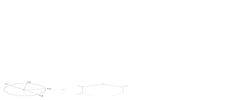
Figure 5: The $n$-point exchange in the low-energy covariantized scattering has the integral form of an $n$-gon integral function in $d$ dimensions.

6 Discussion

In this work we have examined the dual relation between IIB superstring theory and ${\cal N}=4$ super Yang-Mills theory, exploring a number of issues: 1) a formulation of the ${\cal N}=4$ gauge theory which is $S$-dual to the planar limit, 2) the implications of the former for the genus truncation property of the IIB superstring theory at finite couplings, 3) the space-time structure of contributions to the correlation functions in the gauge theory arising from string theory, 4) the pole structure of the OPE for these correlators, 5) features associated with infinite $N_{c}$ and unitarity in the correspondence including one-parameter integrations associated with correlators in accord with Källen-Lehmann representations.

The determination of the space-time integral forms and the coupling structure is a step towards finding the operator product expansion in ${\cal N}=4$ super Yang-Mills theory at intermediate values of the coupling constants. Given the strong form of the AdS/CFT duality and the self-equivalence of IIB superstring theory, the OPE structure is related to the string scattering at different energy scales. We have not analyzed the non-analytic terms in the string scattering in detail within this work, but rather the class of polynomial terms occuring in the expansion of the string S-matrix. These terms generate a class of configuration space triangle diagrams on the field theory side (generally box diagrams, which due to conformal invariance may reduced to triangle diagrams by performing an inversion), whose form suggests that these integral functions are dual to the weak-coupling Feynman diagrams contributing to the correlation function.

The one-parameter integral representations in Section 4 of the large $N$ limit representing the space-time results on the boundary resemble Källen-Lehmann forms in perturbative supersymmetric Yang-Mills theory. By virtue of the strong form of the duality, the infinite curvature limit corresponds to free-field results for the correlators. A deduction of Feynman diagram representations of the correlators in this limit would demonstrate the duality at different regions in coupling space. The presence of non-renormalization theorems indicates that this limit can be taken.

The constraints of $S$-duality and kinematics imply many features of the superstring scattering and the ${\cal N}=4$ gauge theory. In particular, S-duality indicates additional cancellations in the truncation of the IIB superstring to its massless modes in backgrounds preserving all of the supersymmetry. Via the strong form of the AdS/CFT correspondence, this is supported by the existence of an S-dual of the planar expansion in ${\cal N}=4$ super Yang-Mills theory.

In the $S$-dual of the ’t Hooft limit there is no classical supergravity description. However in this limit the coupling structure is such that the superstring theory is potentially to be described by ${\cal N}=4$ topological string calculations [22]. This relation between the $S$-dual limit and the ${\cal N}=4$ topological string theory indicates that there may be a simple description of non-supersymmetric gauge theory in this strong-coupling regime, which may be obtained by a resummation of the perturbative regime or by a string description.

Acknowledgements

The work of G.C. is supported in part by the U.S. Department of Energy, Division of High Energy Physics, Contract W-31-109-ENG-38. J.E., who is a DFG Emmy Noether fellow, acknowledges funding through a DAAD postdoctoral fellowship. G.C. thanks David Kutasov for a useful discussion.

7 Appendix

7.1 $t^{8}$ tensor

The tensor $t^{8}$ has the explicit form

$$t^{8,\mu_{1}\nu_{1}\mu_{2}\nu_{2}\mu_{3}\nu_{3}\mu_{4}\nu_{4}}=-{1\over 2}\epsilon^{\mu_{1}\nu_{1}\mu_{2}\nu_{2}\mu_{3}\nu_{3}\mu_{4}\nu_{4}}$$

$$-{1\over 2}\Bigl{[}(\eta^{\mu_{1}\mu_{2}}\eta^{\nu_{1}\nu_{2}}-\eta^{\mu_{1}\nu_{2}}\eta^{\mu_{2}\nu_{1}})(\eta^{\mu_{3}\mu_{4}}\eta^{\nu_{3}\nu_{4}}-\eta^{\mu_{3}\nu_{4}}\eta^{\mu_{4}\nu_{3}})+(2\leftrightarrow 3),(2\leftrightarrow 4)\Bigr{]}$$

$$+{1\over 2}\Bigl{[}\eta^{\nu_{1}\mu_{2}}\eta^{\nu_{2}\mu_{3}}\eta^{\nu_{3}\mu_{4}}\eta^{\nu_{4}\mu_{1}}+(1\leftrightarrow 2),(2\leftrightarrow 3)+{\rm anti-}(\mu_{j}\leftrightarrow\nu_{j})\Bigr{]}\,.$$ (7.1)

The component of the tensor containing the epsilon tensor does not contribute when restricted to the bulk five-dimensional anti-de Sitter space.

7.2 Terms necessary for determining the space-time dependence

$${\cal E}_{ij,kl}{\cal I}^{R}_{0msklrn0}(z-\vec{x})$$ (7.2)

$$= {\cal E}_{ij,kl}\left[-\frac{1}{16}\frac{1}{d^{2}(d+1)(d-1)(d-2)}\delta_{mn}\partial^{x}_{k}\partial^{x}_{l}\partial^{x}_{r}\partial^{x}_{s}\frac{z_{0}^{d}}{(z-\vec{x})^{2(d-2)}}\right.$$

$$- \frac{1}{8}\frac{1}{d^{2}(d-1)(d+1)}\delta_{mn}\delta_{rs}\partial_{k}\partial_{l}\frac{z_{0}^{d}}{(z-\vec{x})^{2(d-1)}}$$

$$+ \frac{1}{8}\frac{1}{d^{2}(d+1)}\delta_{mn}\delta_{rk}\partial_{s}\partial_{l}\frac{z_{0}^{d}}{(z-\vec{x})^{2(d-1)}}$$

$$+ \frac{1}{2}\frac{1}{d(d+1)}\delta_{mk}\delta_{nl}\partial_{r}\partial_{s}\frac{z_{0}^{(d+2)}}{(z-\vec{x})^{2d}}$$

$$- \left.\frac{1}{4}\frac{(d-1)}{d(d+1)}\delta_{mk}\delta_{nl}\delta_{rs}\frac{z_{0}^{d}}{(z-\vec{x})^{2d}}+\frac{1}{2(d+1)}\delta_{mk}\delta_{nl}\delta_{rs}\frac{z_{0}^{d+2}}{(z-\vec{x})^{2(d+1)}}\right]$$

$$- (m\leftrightarrow s,n\leftrightarrow r)\,,$$

$${\cal E}_{ij,kl}{\cal I}^{R}_{0msklr00}(z-\vec{x})$$ (7.3)

$$= {\cal E}_{ijkl}\left[\frac{(-1)}{2(d+1)}\delta_{lr}\delta_{k[s}\partial^{x}{}_{m]}\frac{z_{0}^{d+1}}{(z-\vec{x})^{2d}}+\frac{1}{(d+1)}\delta_{lr}\delta_{k[m}\partial^{x}_{s]}\frac{z_{0}^{d+3}}{(z-\vec{x})^{2(d+1)}}\right.$$

$$+ \left.\frac{1}{4(d-1)d(d+1)}\delta_{k[m}\partial_{s]}\partial_{l}\partial_{r}\frac{z_{0}^{d+1}}{(z-\vec{x})^{2(d-1)}}+\frac{1}{2(d+1)}\delta_{k[m}\delta_{s]r}\partial_{l}\frac{z_{0}^{d+1}}{(z-\vec{x})^{2d}}\right]\quad,$$

$${\cal E}_{ij,kl}{\cal I}^{R}_{00sklr00}(z-\vec{x})$$ (7.4)

$$= {\cal E}_{ij,kl}\left[\frac{1}{16d^{2}(d-2)(d+1)}\partial_{r}^{x}\partial_{s}^{x}\partial_{k}^{x}\partial_{l}^{x}\frac{z_{0}^{d}}{(z-\vec{x})^{2(d-2)}}\right.$$

$$- \frac{1}{8d^{2}(d-1)(d+1)}\left(\delta_{sk}\partial_{r}\partial_{l}\frac{z_{0}^{d}}{(z-\vec{x})^{2(d-1)}}+\delta_{rl}\partial_{s}\partial_{k}\frac{z_{0}^{d}}{(z-\vec{x})^{2(d-1)}}\right)$$

$$+ \frac{1}{4}\frac{1}{d(d+1)}\left(\delta_{sk}\partial_{r}\partial_{l}\frac{z_{0}^{d+2}}{(z-\vec{x})^{2d}}+\delta_{rl}z_{0}^{d+2}\partial_{s}\partial_{k}\frac{1}{(z-\vec{x})^{2d}}\right)$$

$$+ \frac{1}{4}\frac{1}{(d-1)^{2}d(d+1)}\delta_{rk}\delta_{sl}\frac{z_{0}^{d}}{(z-\vec{x})^{2d}}-\frac{d}{(d+1)}\frac{z_{0}^{d+2}}{(z-\vec{x})^{2(d+1)}}\delta_{rk}\delta_{sl}+\frac{z_{0}^{d+4}}{(z-\vec{x})^{2(d+2)}}\delta_{rk}\delta_{sl}$$

$$- \left.\frac{1}{4d^{2}(d+1)}z_{0}^{d+2}\delta_{rs}\partial_{k}\partial_{l}\frac{1}{(z-\vec{x})^{2d}}+\frac{1}{8d^{2}(d+1)}\delta_{rs}z_{0}^{d}\partial_{k}\partial_{l}\frac{1}{(z-\vec{x})^{2(d-1)}}\right]\,.$$

7.3 Box diagrams

The general box diagram required for the evaluation of the finite $\lambda$ and $N$ results is of the form,

$$I_{a;a_{j}}^{\gamma}=\int{dz_{0}d^{d}{\vec{z}}\over z_{0}^{d+1}}~{}z_{0}^{\gamma}\times\prod_{j=1}^{4}\Bigl{[}{z_{0}^{d+a_{j}}\over(z-{\vec{x}}_{j})^{2d+2a_{j}}}\Bigr{]}\ ,$$ (7.5)

with $\gamma=a+m-\sum_{j=1}^{4}a_{j}$. The integral form in (7.5) is of a box diagram with $d+a_{j}$ powers of propagators on each internal line. We may express the integral in a more conformal field notation via

$$I_{a;a_{j}}^{\gamma}=\int{dz_{0}d^{d}{\vec{z}}\over z_{0}^{d+1}}~{}z_{0}^{\gamma}\times\prod_{j=1}^{4}\Bigl{[}{z_{0}^{\Delta_{j}}\over(z-{\vec{x}}_{j})^{2\Delta_{j}}}\Bigr{]}\ ,$$ (7.6)

with $\Delta_{j}=d+a_{j}$. The conformal invariance at $\gamma=0$ of the integral demands the structure,

$$I_{a;a_{j}}^{0}=F(\zeta,\eta)\times\prod_{i<j}(x_{ij}^{2})^{-{{\Delta_{i}+\Delta_{j}}\over 2}+{1\over 6}\sum_{j=1}^{4}\Delta_{j}}\ ,$$ (7.7)

with the two independent scalar conformal invariant cross ratios in (5.30).

The Schwinger parameterization of the integrals in (7.5) leads to the integral form,

$$I_{a;a_{j}}^{\gamma}=C_{a;a_{j}}^{\gamma}\int\prod_{j=1}^{4}d\alpha_{j}~{}\delta(1-\sum\alpha_{i})~{}M^{\gamma\over 2}~{}{\alpha_{j}^{\Delta_{j}-1}\over M^{{1\over 2}\sum_{j=1}^{4}\Delta_{j}}}\ ,$$ (7.8)

with

$$C_{a;a_{j}}^{\gamma}={1\over 2}\Omega_{d+1}^{(a+m)}{\Gamma(2d+{a+m\over 2})\Gamma(2d-{\gamma\over 2}+{1\over 2}\sum a_{j})\over\prod_{j=1}^{4}\Gamma(d+a_{j})}$$ (7.9)

and

$$M=\sum_{i\neq j}^{4}\alpha_{i}\alpha_{j}x_{ij}^{2}\ .$$ (7.10)

The $M^{\gamma/2}$ factor represents the difference from the standard four-point scalar conformal diagram without any derivatives, i.e. the box diagram. Note that with non-zero $\gamma$ the form in (7.8) is that of a conformal box diagram evaluated in dimension $d=4-a+\sum a_{j}$.

The integrals in (7.5) for $\gamma=0$ are finite; the range of $a_{j}$ is $|a_{j}|\leq 2$ and for $d\geq 4$ the arguments of the gamma functions are finite. However, for large enough values of $\gamma$, the prefactor in $C_{a;a_{j}}^{\gamma}$ develops a pole after regulating, for example, with dimensional continuation ($d=m-\epsilon$ and $m$ integer); the origin of this pole is an ultra-violet divergence found in standard field theory by integrating a box diagram with multiple insertions of loop momenta in the numerator. For this reason the integrals in these cases have to be evaluated to first order in $\epsilon$.

We note that in $d=4$ and for $\gamma=0$ the integrals above may be found by multiple differentiation with respect to ${\vec{x}}_{ij}^{2}$ of the scalar box function

$$B=\int\prod d\alpha_{j}~{}{\delta(1-\sum\alpha_{j})\over(\mathop{\sum}_{i\neq j}\alpha_{i}\alpha_{j}{\vec{x}}_{ij}^{2})^{2}}\ .$$ (7.11)

References

- [1] J. Maldacena, Adv. Theor. Math. Phys. 2, 231 (1998) [hep-th/9711200].
- [2] S. S. Gubser, I. R. Klebanov and A. M. Polyakov, Phys. Lett. B428, 105 (1998) [hep-th/9802109].
- [3] E. Witten, Adv. Theor. Math. Phys. 2, 253 (1998) [hep-th/9802150].
- [4] O. Aharony, S. S. Gubser, J. Maldacena, H. Ooguri and Y. Oz, [hep-th/9905111].
- [5] D. Z. Freedman, S. D. Mathur, A. Matusis and L. Rastelli, Nucl. Phys. B546, 96 (1999) [hep-th/9804058].
- [6] W. Muck and K. S. Viswanathan, Phys. Rev. D58, 041901 (1998) [hep-th/9804035].
- [7] G. Chalmers, H. Nastase, K. Schalm and R. Siebelink, Nucl. Phys. B540, 247 (1999) [hep-th/9805105].
- [8] S. Lee, S. Minwalla, M. Rangamani and N. Seiberg, Adv. Theor. Math. Phys. 2, 697 (1998) [hep-th/9806074].
- [9] E. D’Hoker, D. Z. Freedman and W. Skiba, Phys. Rev. D59, 045008 (1999) [hep-th/9807098].
- [10] W. Skiba, Phys. Rev. D60, 105038 (1999) [hep-th/9907088].
- [11] E. D’Hoker, D. Z. Freedman, S. D. Mathur, A. Matusis and L. Rastelli, hep-th/9908160.
- [12] M. Bianchi and S. Kovacs, Phys. Lett. B468, 102 (1999) [hep-th/9910016].
- [13] J. Erdmenger and M. Pérez-Victoria, hep-th/9912250, to appear in Phys. Rev. D.
- [14] E. D’Hoker, J. Erdmenger, D. Z. Freedman and M. Pérez-Victoria, hep-th/0003218.
- [15] B. U. Eden, P. S. Howe, E. Sokatchev and P. C. West, hep-th/0004102.
- [16] G. Chalmers, to appear in Nuclear Physics B, hep-th/0001190.
- [17] T. Banks and M. B. Green, JHEP 9805, 002 (1998) [hep-th/9804170].
- [18] M. B. Green and M. Gutperle, Nucl. Phys. B498, 195 (1997), [hep-th/9701093].
- [19] K. Intriligator, Nucl. Phys. B551, 575 (1999) [hep-th/9811047].
- [20] K. Intriligator and W. Skiba, Nucl. Phys. B559, 165 (1999) [hep-th/9905020].
- [21] J. H. Brodie and M. Gutperle, Phys. Lett. B445, 296 (1999) [hep-th/9809067].
- [22] N. Berkovits and C. Vafa, Nucl. Phys. B533 (1998) 181 [hep-th/9803145].
- [23] N. Berkovits, Proceedings Strings ’98, http://www.itp.ucsb.edu/online/strings98.
- [24] J. G. Russo, Phys. Lett. B417, 253 (1998) [hep-th/9707241].
- [25] J. G. Russo, Nucl. Phys. B535, 116 (1998) [hep-th/9802090].
- [26] G. Chalmers and K. Schalm, JHEP 9910, 016 (1999) [hep-th/9909087].
- [27] M. B. Green, H. Kwon and P. Vanhove, Phys. Rev. D61, 104010 (2000) [hep-th/9910055].
- [28] M. B. Green and S. Sethi, Phys. Rev. D59, 046006 (1999) [hep-th/9808061].
- [29] N. A. Obers and B. Pioline, Commun. Math. Phys. 209, 275 (2000) [hep-th/9903113].
- [30] N. A. Obers and B. Pioline, Phys. Rept. 318, 113 (1999) [hep-th/9809039].
- [31] R. Gopakumar and M. B. Green, JHEP 9912, 015 (1999) [hep-th/9908020].
- [32] M. Bianchi, M. B. Green, S. Kovacs and G. Rossi, JHEP 9808, 013 (1998) [hep-th/9807033].
- [33] N. Dorey, V. V. Khoze, M. P. Mattis and S. Vandoren, Phys. Lett. B442, 145 (1998) [hep-th/9808157].
- [34] N. Dorey, T. J. Hollowood, V. V. Khoze, M. P. Mattis and S. Vandoren, Nucl. Phys. B552, 88 (1999) [hep-th/9901128].
- [35] A. V. Belitsky, S. Vandoren and P. van Nieuwenhuizen, hep-th/0004186.
- [36] N. Berkovits and C. Vafa, Nucl. Phys. B433 (1995) 123 [hep-th/9407190].
- [37] T. Eguchi, hep-th/9804037.
- [38] G. ’t Hooft, Commun. Math. Phys. 86, 449 (1982).
- [39] Z. Bern, L. Dixon, D. C. Dunbar, M. Perelstein and J. S. Rozowsky, Nucl. Phys. B530, 401 (1998) [hep-th/9802162].
- [40] H. Liu and A. A. Tseytlin, Phys. Rev. D59, 086002 (1999) [hep-th/9807097].
- [41] G. Chalmers and K. Schalm, Nucl. Phys. B554, 215 (1999) [hep-th/9810051].
- [42] E. D’Hoker and D. Z. Freedman, Nucl. Phys. B550, 261 (1999) [hep-th/9811257].
- [43] E. D’Hoker, D. Z. Freedman, S. D. Mathur, A. Matusis and L. Rastelli, Nucl. Phys. B562, 330 (1999) [hep-th/9902042].
- [44] E. D’Hoker, D. Z. Freedman, S. D. Mathur, A. Matusis and L. Rastelli, Nucl. Phys. B562, 353 (1999) [hep-th/9903196].
- [45] G. Chalmers, hep-th/9907015.
- [46] H. Liu, Phys. Rev. D60, 106005 (1999) [hep-th/9811152].
- [47] D. Anselmi, Class. Quant. Grav. 17, 1383 (2000) [hep-th/9906167].
- [48] E. D’Hoker, S. D. Mathur, A. Matusis and L. Rastelli, hep-th/9911222.
- [49] L. Hoffmann, A. C. Petkou and W. Rühl, hep-th/0002154, hep-th/0002025.
- [50] I.M. Gel’fand and G.E. Shilov, Generalized Functions, Vol. I: Properties and Operations. Academic Press, New York and London, 1964.
- [51] H. Osborn and A. C. Petkou, Annals Phys. 231, 311 (1994) [hep-th/9307010].
- [52] J. Erdmenger and H. Osborn, Nucl. Phys. B483, 431 (1997) [hep-th/9605009].
- [53] G. Arutyunov and S. Frolov, Phys. Rev. D60, 026004 (1999) [hep-th/9901121].
- [54] H. Liu and A. A. Tseytlin, Nucl. Phys. B533, 88 (1998) [hep-th/9804083].
- [55] A. A. Tseytlin, hep-th/0005072.
- [56] C. Anastasiou, E. W. Glover and C. Oleari, Nucl. Phys. B572, 307 (2000) [hep-ph/9907494].
- [57] E. E. Boos and A. I. Davydychev, Theor. Math. Phys. 89, 1052 (1991).