KUNS-1665 hep-th/0005178
Scalar field theories in a Lorentz-invariant three-dimensional noncommutative space-time

We discuss scalar quantum field theories in a Lorentz-invariant three-dimensional noncommutative space-time. We first analyse the one-loop diagrams of the two-point functions, and show that the non-planar diagrams are finite and have infrared singularities from the UV/IR mixing. The scalar quantum field theories have the problem that the violation of the momentum conservation from the non-planar diagrams does not vanish even in the commutative limit. A way to obtain an exact translational symmetry by introducing an infinite number of tensor fields is proposed. The translational symmetry transforms local fields into non-local ones in general. We also discuss an analogue of thermodynamics of free scalar field theory in the noncommutative space-time.

1 Introduction

Quantum field theories in noncommutative space-times with the noncommutativity $[x^{\mu},x^{\nu}]=i\theta^{\mu\nu}$ are interesting in pursuing the new possibilities of quantum field theories in quantum space-times. Remarkably, this kind of noncommutativity between coordinates appears in string theory, for instance, in the toroidal compactification of Matrix Theory [1] and in open string theory [3]-[7] with a B-field background. Thus it may be expected that field theories in this kind of noncommutative space-times are controllable in some way. On the other hand, however, perturbative analyses show that these noncommutative field theories have interesting but unusual behaviours [8]-[21]. Infrared singularities in the correlation functions were shown to appear even for massive theories [8]-[11]. In the case with space-time noncommutativity with $\theta^{0i}\neq 0$ [15]-[18], the causality is violated in interesting ways [15], and S-matrix does not satisfy unitarity constraints [18]. Thus, before we become able to handle such noncommutative quantum field theories consistently, there still seems to remain a lot to learn about them.

An obvious direction to learn more would be to generalise the class of noncommutative space-time. A constant background of $\theta^{\mu\nu}$ violates Lorentz symmetry in more than two-dimensional space-time. Since Lorentz symmetry is one of the fundamental components in the present theoretical physics, in this paper we consider a Lorentz-invariant three-dimensional space-time with the noncommutativity $[x^{\mu},x^{\nu}]=2i\l_{P}\varepsilon^{\mu\nu\rho}x_{\rho}$. Though this noncommutativity is different from that obtained from the constant background of the two-form field in string theory, a similar kind of noncommutativity between more than two coordinates appears on the boundary string of a membrane in M-theory with a non-vanishing background of the three-form field [26, 27], and also on a D2-brane in a non-constant two-form field background in string theory [28]. Another motivation comes from that this noncommutative space-time may be regarded as a fuzzy space-time with a Lorentz-invariant space-time uncertainty relation [29] derived from a gedanken experiment in which only the general relativity and quantum mechanics are used [30]-[34]. Concerning the questions whether there is any relationship between the space-time uncertainty relation and quantum gravity or string theory [35], as well as whether the properties obtained so far for the specific noncommutative quantum field theories are general in other noncommutative space-times, it would be interesting to investigate quantum field theories in that noncommutative three-dimensional space-time. As for the latter question, since the time-coordinate is also noncommutative in the space-time we consider, it should be the most radical case with the above-mentioned violations of causality and unitarity [15]-[18]. In this paper, we shall discuss only scalar field theories in the noncommutative space-time.

The organisation of this paper is as follows. In section 2, we discuss the group theoretical structure of the one-particle Hilbert space of free scalar field theory. In section 3, we define the action and derive the Feynman rules. In section 4, we compute some one-loop diagrams. The non-planar diagrams are shown to be finite and have infrared singularities from the UV/IR mixing. We encounter the feature that the violation of the momentum conservation from the non-planar diagrams does not vanish even in the commutative limit $l_{P}\rightarrow 0$. In section 5, we propose a translationally symmetric theory to remedy the defect. In section 6, we discuss a noncommutative analogue of the thermodynamics of free scalar field theory and compare the result with the qualitative estimation given previously in [32]. Section 7 is devoted for the summary and discussions.

2 One-particle Hilbert space

In the paper [29], one of the present authors discussed the momentum space representation of the one-particle Hilbert space of free scalar field theory in a Lorentz-invariant three-dimensional noncommutative space-time. There the noncommutativity of the space-time is motivated by a space-time uncertainty relation derived from a certain gedanken experiment [29]-[32]. In this section we discuss the group theoretical structure of the one-particle Hilbert space.

2.1 Construction via $ISO(2,2)$ algebra

The three-dimensional noncommutative space-time in [29] is represented by the following $SO(1,2)$ Lorentz-invariant commutation relations between the coordinates and momentum operators:

$$[\hat{x}^{\mu},\hat{x}^{\nu}] = 2il_{P}\epsilon^{\mu\nu\rho}\hat{x}_{\rho},$$ (1)

$$[\hat{p}^{\mu},\hat{p}^{\nu}] = 0,$$ (2)

$$[\hat{p}^{\mu},\hat{x}^{\nu}] = -i\eta^{\mu\nu}\sqrt{1+l_{P}^{2}\hat{p}^{2}}+il_{P}\epsilon^{\mu\nu\rho}\hat{p}_{\rho},$$ (3)

where the greek indices run through 0 to 2, and the numerical constant $l_{P}$ should be in the order of Planck length.

Now let us consider the lie algebra of $ISO(2,2)$,

$$[\hat{J}_{mn},\hat{J}_{kl}] = -i(\eta_{mk}\hat{J}_{nl}-\eta_{ml}\hat{J}_{nk}-\eta_{nk}\hat{J}_{ml}+\eta_{nl}\hat{J}_{mk}),$$ (4)

$$[\hat{J}_{mn},\ \hat{p}_{k}] = -i(\eta_{mk}\hat{p}_{n}-\eta_{nk}\hat{p}_{m}),$$ (5)

$$[\ \hat{p}_{m},\ \hat{p}_{n}] = 0,$$ (6)

where the roman indices run through $-1$ to 2, and the signature is given by $\eta_{mn}=(-,-,+,+)$. By identifying

$$\hat{x}_{\mu} = l_{P}(\hat{J}_{-1,\mu}-\frac{1}{2}\epsilon_{\mu}{}^{\alpha\beta}\hat{J}_{\alpha\beta}),$$ (7)

$$\hat{p}_{\mu} = \hat{p}_{m=\mu},$$ (8)

and imposing a constraint

$$1+l_{P}^{2}\hat{p}^{m}\hat{p}_{m}=0,$$ (9)

we can easily show that the commutation relations (1) can be derived from (4). The momentum square $\hat{p}^{m}\hat{p}_{m}$ is one of the Casimir operators of the algebra (4), and hence we may consistently impose the constraint (9). The remaining three independent generators in (4) are now the $SO(1,2)$ Lorentz generators of the noncommutative space-time (1).

The representation of the algebra (1) is obtained from that of $ISO(2,2)$, which is given by $\hat{J}_{mn}=i(p_{m}\frac{\partial}{\partial p^{n}}-p_{n}\frac{\partial}{\partial p^{m}})$ in the momentum space representation. In order to impose the constraint (9), the following “polar” coordinate is convenient:

$$p_{-1} = r{\rm cosh}\chi\cos\theta,$$ (10)

$$p_{0} = r{\rm cosh}\chi\sin\theta,$$ (11)

$$p_{1} = r{\rm sinh}\chi\cos\phi,$$ (12)

$$p_{2} = r{\rm sinh}\chi\sin\phi.$$ (13)

This coordinate is only valid in the neighbourhood of the hyperboloid $1+l_{P}^{2}p^{m}p_{m}=0$, but this is enough for our purposes. Since $\hat{J}_{mn}p^{l}p_{l}=0$ and $\hat{J}_{mn}$ do not contain $r$-derivative, we can restrict the representation space to the functions on the hyperboloid, i.e. the functions depending only on $\chi,\theta,\phi$. Thus the natural inner-product that makes $\hat{J}_{mn},\hat{p}_{m}$ hermite in the restricted representation space is given by

$$\langle\Phi_{1}|\Phi_{2}\rangle=2\int d^{4}p\ \delta(1+l_{P}^{2}p^{m}p_{m})\Phi_{1}^{*}(p)\Phi_{2}(p).$$ (14)

After integrating over $p_{-1}$, this inner product is identical to that obtained previously in [29].

The constraint (9) shows that the mass square $-p^{\mu}p_{\mu}$ in the noncommutative space-time should have an upper bound $-p^{\mu}p_{\mu}\leq 1/l_{P}^{2}$, and also that, coming from the choices of the sign of $p_{-1}$, there exists two-fold degeneracy in the momentum space of the noncommutative space-time. These features agree with the results obtained in [29].

2.2 $SL(2,R)$ structure of the momentum space

In the previous subsection, we have shown that the momentum space is the hyperboloid, $1+l_{P}^{2}p^{m}p_{m}=0$. This hyperboloid can be mapped to the group manifold $SL(2,R)$ as follows. Let us define the matrices

$${\mathbb{x}}^{0} = l_{P}\sigma^{2}=l_{P}\left(\matrix{0&-i\cr i&0}\right),$$ (15)

$${\mathbb{x}}^{1} = l_{P}i\sigma^{3}=l_{P}\left(\matrix{i&0\cr 0&-i}\right),$$ (16)

$${\mathbb{x}}^{2} = l_{P}i\sigma^{1}=l_{P}\left(\matrix{0&i\cr i&0}\right),$$ (17)

which satisfy

$${\mathbb{x}}^{\mu}{\mathbb{x}}^{\nu}=-l_{P}^{2}\eta^{\mu\nu}+il_{P}\epsilon^{\mu\nu\lambda}{\mathbb{x}}_{\lambda}.$$ (18)

Then the map between the hyperboloid and the group elements of $SL(2,R)$ is defined by

$$g=l_{P}\left(\matrix{p_{-1}-p_{1}&p_{0}-p_{2}\cr-p_{0}-p_{2}&p_{-1}+p_{1}}\right)=l_{P}p_{-1}+i{\mathbb{x}}^{\mu}p_{\mu}=e^{ik{\mathbb{x}}}.$$ (19)

By a direct computation, we can verify $p_{\mu}=k_{\mu}{\rm sinh}(l_{P}\sqrt{k^{2}})/l_{P}\sqrt{k^{2}}$. As discussed in [29], this relation is identical to the relation between $k_{\mu}$ and the $\hat{p}_{\mu}$-eigenvalue of the state $e^{-ik\hat{x}}|0\rangle$, where $|0\rangle$ denotes the momentum-zero eigen-state with $p_{-1}=1$. Thus the one-particle Hilbert space can be parameterised by the group manifold $SL(2,R)$:

$$|p(g)\rangle=e^{ik(g)\hat{x}}|0\rangle,$$ (20)

where $p_{m}(g)$ and $k_{\mu}(g)$ are defined by (19). This parameterisation with $SL(2,R)$ elements is superior to the parameterisation by the space-time momentum $p_{\mu}$, because distinct choices of the signs of $p_{-1}$ correspond to distinct group elements and we do not need to worry about the two-fold degeneracy in the momentum space representation.

For later convenience, we collect some useful formulae in the followings. From (18) and (19), we can show that the group multiplication can be expressed in terms of $p_{m}$ by

$$p(gh)_{-1} = l_{P}(p(g)_{-1}p(h)_{-1}+p(g)^{\alpha}p(h)_{\alpha}),$$ (21)

$$p(gh)_{\mu} = l_{P}(p(g)_{-1}p(h)_{\mu}+p(g)_{\mu}p(h)_{-1}-\epsilon_{\mu}{}^{\alpha\beta}p(g)_{\alpha}p(h)_{\beta}).$$ (22)

Note that ${\rm tr}(g)=2p(g)_{-1}=\pm 2\sqrt{l_{P}^{-2}+p_{\mu}(g)p^{\mu}(g)}$. Since an adjoint action keeps the trace invariant, it keeps $p_{\mu}p^{\mu}$ invariant. Hence the adjoint action of $SL(2,R)$ corresponds to the $SO(1,2)$ Lorentz transformation of the space-time. Under the adjoint action, $p(h)_{m}$ transforms as

$$p(g^{-1}hg)_{-1} = p(h)_{-1},$$ (23)

$$p(g^{-1}hg)_{\mu} = p(h)_{\mu}(1+2a^{\alpha}a_{\alpha})-2p(h)^{\alpha}a_{\alpha}a_{\mu}-2\epsilon_{\mu}{}^{\alpha\beta}p(h)_{\alpha}a_{\beta}a_{-1},$$ (24)

where $a_{m}=l_{P}p(g)_{m}$.

After a short computation, we can verify that the inner product defined in (14) is just the integration over the $SL(2,R)$ group manifold with the invariant measure,

$$d\mu(g)=\frac{1}{2\ 3!}{\rm tr}(g^{-1}dg)^{3}=2d^{4}p\ \delta(1+l_{P}^{2}p^{m}p_{m}).$$ (25)

Hence we have

$$d\mu(g)=d\mu(gh)=d\mu(hg).$$ (26)

The above formulas will be used in computing one-loop diagrams in section 4.

3 Action and Feynman rules

In this section, we construct the actions of interacting scalar field theories in the noncommutative space-time and derive the Feynman rules.

A scalar field in the noncommutative space-time is defined by associating momentum space wave functions $\Phi(g)$ to “vertex operators” as follows:

$$\hat{\Phi} = \int d\mu(g)\Phi(g)e^{ik(g)\hat{x}},$$ (27)

$$|\Phi\rangle = \int d\mu(g)\Phi(g)e^{ik(g)\hat{x}}|0\rangle=\int d\mu(g)\Phi(g)|p(g)\rangle,$$ (28)

where $p(g)$ and $k(g)$ are defined by (19). We impose the reality condition on the field $\hat{\Phi}$, i.e. $\hat{\Phi}^{\dagger}=\hat{\Phi}$. We can define the product of the vertex operators by Hausdorff formula, following the line of [25]. Since the Hausdorff formula is nothing but the group multiplication, we obtain

$$e^{ik(g_{1})\hat{x}}*e^{ik(g_{2})\hat{x}}=e^{ik(g_{1}g_{2})\hat{x}}.$$ (29)

Making use of this $*$-product, we can construct interaction terms. For example, the action of noncommutative $\phi^{3}$-theory can be defined in the following way:

$$S[\Phi]=\frac{-1}{2}\langle 0|\hat{\Phi}*(\hat{p}^{2}+m^{2})\hat{\Phi}|0\rangle+\frac{\lambda}{3}\langle 0|\hat{\Phi}*\hat{\Phi}*\hat{\Phi}|0\rangle,$$ (30)

where $\hat{p}^{2}=\hat{p}_{\mu}\hat{p}^{\mu}$.

For practical computation, it is convenient to rewrite this action in the momentum space representation with $SL(2,R)$ elements, and, for this, we need to evaluate $\langle 0|e^{ik(g)\hat{x}}|0\rangle=\langle 0|p(g)\rangle$. From the definition of the inner product, we can show that $\langle 0|p(g)\rangle$ is a $\delta$-function with respect to the invariant measure $d\mu(g)$, which has a support at the unit element of $SL(2,R)$:

$$\langle 0|\Phi\rangle\equiv\int d\mu(g)\langle 0|p(g)\rangle\langle p(g)|\Phi\rangle\Leftrightarrow\Phi(g=1)=\int d\mu(g)\langle 0|p(g)\rangle\Phi(g).$$ (31)

Henceforth, we denote this $\delta$-function as $\delta(g)$.

Now we can write down the momentum representation of the action as

$$S[\Phi] = \frac{-1}{2}\langle 0|\hat{\Phi}*(\hat{p}^{2}+m^{2})\hat{\Phi}|0\rangle+\frac{\lambda}{3}\langle 0|\hat{\Phi}*\hat{\Phi}*\hat{\Phi}|0\rangle$$ (32)

$$= \frac{-1}{2}\int d\mu(g)\Phi(g^{-1})(p^{2}(g)+m^{2})\Phi(g)$$ (34)

$$+\frac{\lambda}{3}\int\prod_{i=1}^{3}d\mu(g_{i})\delta(g_{1}g_{2}g_{3})\Phi(g_{1})\Phi(g_{2})\Phi(g_{3}).$$

Assuming an appropriate path integral measure, we can perform perturbative computation.

$$Z[J] = \int[D\Phi]\exp\left(iS_{\rm free}[\Phi]+iS_{\rm int}[\Phi]+i\int d\mu(g)J(g^{-1})\Phi(g)\right)$$ (35)

$$= \exp\left(iS_{\rm int}\left[\frac{\delta}{i\delta J}\right]\right)\exp\left(\frac{1}{2}\int d\mu(g)\ iJ(g^{-1})\frac{-i}{p^{2}(g)+m^{2}}iJ(g)\right)$$ (37)

$$\times\int[D\Phi]\exp\left(\frac{i}{2}\int d\mu(g)(\Phi-\frac{1}{p^{2}+m^{2}}J)(p^{2}+m^{2})(\Phi-\frac{1}{p^{2}+m^{2}}J)\right)$$

We may assume the last Gaussian path integral just gives a constant. Thus, generalising to arbitrary $\phi^{n}$ interactions, we obtain the following Feynman rules,

$${\rm propagator}: \int d\mu(g)\frac{-i}{p^{2}(g)+m^{2}},$$ (38)

$$n{\rm-vertex}: i\lambda_{n}\delta(g_{1}\dots g_{n})$$ (39)

Note that, since momentums are $SL(2,R)$ elements, we have noncommutativity at the vertex. In the following section, we compute some one-loop diagrams, using these rules.

4 One-loop computation

In this section we shall compute the one-loop diagrams of the two-point functions from $\phi^{3}$ and $\phi^{4}$-interactions defined in the previous section. We will show that the non-planar one-loop diagrams are finite and have infrared singularities from the UV/IR mixing [8]-[11]. We will also find that those diagrams cause a problem concerning the conservation of momentums. In this section, we set $l_{P}=1$ for simplicity.

4.1 The planar diagram of the two-point function from $\phi^{4}$-interaction

In the first place, we shall compute the simplest graph to show our computational strategy: the one-loop planar diagram of the two-point function from $\phi^{4}$-interaction as in fig.(1).

Figure 1: The one-loop planar diagram of the two-point function.

From the Feynman rules in the preceding section, the amplitude of this diagram is given by

$$\Gamma^{(2)}_{P} = \int d\mu(g)i\delta(g^{-1}h_{2}h_{1}g)\frac{-i}{p^{2}(g)+m^{2}}=\delta(h_{2}h_{1})\int d\mu(g)\frac{1}{p^{2}(g)+m^{2}}.$$ (40)

The polar coordinate (10) is convenient for the explicit evaluation of this integral, and we further perform the change of the variable, $x={\rm cosh}^{2}\chi$. With this parameterisation, we obtain

$$p(g) = (x^{\frac{1}{2}}\sin\theta,\ (1+x)^{\frac{1}{2}}\cos\phi,\ (1+x)^{\frac{1}{2}}\sin\phi),$$ (41)

$$p^{2}(g)+m^{2} = (p(g)_{-1})^{2}-1+m^{2}=x\cos^{2}\theta-\cos^{2}\mu,$$ (42)

$$d\mu(g) = \int_{0}^{2\pi}d\phi\int_{0}^{2\pi}d\theta\int_{1}^{\infty}\frac{dx}{2},$$ (43)

where $\sin\mu=m\ (0\leq\mu\leq\pi/2)$.

Since this integration turns out to be divergent, we introduce a momentum cut-off $\Lambda$ in the $x$-integration.

$$\Gamma^{(2)}_{P} = \delta(h_{2}h_{1})\int_{0}^{2\pi}d\phi\int_{0}^{2\pi}d\theta\int_{1}^{\Lambda^{2}}\frac{dx}{2}\frac{1}{x\cos^{2}\theta-\cos^{2}\mu}$$ (44)

$$= 2\pi^{2}\ \delta(h_{2}h_{1})\int_{1}^{\Lambda^{2}}\frac{dx}{x}\int_{0}^{2\pi}\frac{id\theta}{2\pi i}\frac{1}{\cos^{2}\theta-\cos^{2}\mu_{x}}$$ (45)

$$= 2\pi^{2}\ \delta(h_{2}h_{1})\int_{1}^{\Lambda^{2}}\frac{dx}{x}\int_{0}^{2\pi}\frac{id\theta}{2\pi i}\frac{1}{\sin(\mu_{x}+\theta)\sin(\mu_{x}-\theta)},$$ (46)

where we have defined $\cos\mu_{x}=\cos\mu/x$.

Figure 2: $(m^{2}-i\epsilon)$-prescription

By the change of the integration variable $z=e^{i\theta}$, the integration over $\theta$ is now a contour integration on a unit circle in the $z$-plane. There are poles at $z=\pm e^{i\mu_{x}},\pm e^{-i\mu_{x}}$. Since they are on the unit circle, we adopt $(m^{2}-i\epsilon)$-prescription to make the integral well-defined. Then we just pick up the residues at $z=\pm e^{-i\mu_{x}}$ as shown in fig.(2). Thus the result of the integration is given by

$$\Gamma^{(2)}_{P} = 2\pi^{2}i\ \delta(h_{2}h_{1})\int_{1}^{\Lambda^{2}}\frac{dx}{x}\frac{x}{\sqrt{x-(1-m^{2})}\sqrt{1-m^{2}}}$$ (47)

$$= -4\pi^{2}i\ \delta(h_{2}h_{1})\left(\sqrt{\frac{m^{2}}{1-m^{2}}}-\sqrt{\frac{\Lambda^{2}}{1-m^{2}}}\right),$$ (48)

where we have neglected the terms that vanish as $\Lambda\rightarrow\infty$. We need to renormalize the divergence of the second term by a mass counter term.

4.2 The non-planar diagram of the two-point function from $\phi^{4}$-interaction

Figure 3: The non-planar one-loop diagram of the two-point function

Next we consider the non-planar diagram of fig.(3). The amplitude is given by

$$\Gamma^{(2)}_{NP}=\int d\mu(g)i\delta(h_{2}g^{-1}h_{1}g)\frac{-i}{p^{2}(g)+m^{2}}.$$ (49)

The integration over $g$ is performed for the solutions to $h_{2}g^{-1}h_{1}g=1$. Thus this integral is non-vanishing only if $h_{1}$ and $h_{2}$ belong to the same conjugacy class, so both $p(h_{1})_{\mu}$ and $p(h_{2})_{\mu}$ must be time-like or space-like, simultaneously. We shall evaluate this integral when both the momentums are time-like. Without loss of generality, we may assume $p(h_{1})_{\mu}$ is in the time direction, and $p(h_{2})_{\mu}$ is represented by a vector obtained by boosting a vector $p(h_{2}^{\prime})_{\mu}$ which is in the time direction:

$$p(h^{\prime}_{2})_{\mu} = (p(h^{\prime}_{2})_{0},\ 0,\ 0),$$ (50)

$$p(h_{2})_{\mu} = p(g_{2}^{-1}h^{\prime}_{2}g_{2})$$ (51)

$$= (p(h^{\prime}_{2})_{0}\ {\rm cosh}2\chi_{2},\ p(h^{\prime}_{2})_{0}\ {\rm sinh}2\chi_{2}\sin\phi_{2},\ -p(h^{\prime}_{2})_{0}\ {\rm sinh}2\chi_{2}\cos\phi_{2}).$$ (52)

We can rewrite

$$\Gamma^{(2)}_{NP} = \int d\mu(g)\delta(h^{\prime}_{2}g_{2}g^{-1}h_{1}gg_{2}^{-1})\frac{1}{p^{2}(g)+m^{2}}$$ (53)

$$= \int d\mu(g)\delta(h^{\prime}_{2}g^{-1}h_{1}g)\frac{1}{p^{2}(gg_{2})+m^{2}},$$ (54)

where we have changed the integration variable $g$ to $gg_{2}$. An adjoint action is simplified when acting on a vector in the time-direction:

$$p(g^{-1}h_{1}g)_{0} = p(h_{1})_{0}(1+2(p_{1}^{2}+p_{2}^{2})),$$ (55)

$$p(g^{-1}h_{1}g)_{i} = 2p(h_{1})_{0}(p_{0}p_{i}+\epsilon_{i}{}^{j}p_{-1}p_{j}),$$ (56)

where we have abbreviated $p_{m}=p(g)_{m}$. We can show the following formula :

$$\delta(gh)=|p(h)_{-1}|\ \theta(p(g)_{-1}p(h)_{-1})\ \delta^{(3)}(p(g)+p(h)).$$ (60)

Making use of it, we obtain

$$\Gamma_{NP}^{2} = |p(h_{1})_{-1}|\ 2\int d^{4}p\ \delta(1+p^{m}p_{m})$$ (62)

$$\ \times\theta(p(g^{-1}h_{1}g)_{-1}p(h^{\prime}_{2})_{-1})\ \delta^{(3)}(p(g^{-1}h_{1}g)+p(h^{\prime}_{2}))\frac{1}{p^{2}(gg_{2})+m^{2}}$$

$$= |p(h_{1})_{-1}|\ 2\int d^{4}p\ \delta(1+p^{m}p_{m})$$ (65)

$$\ \times\theta(p(h_{1})_{-1}p(h^{\prime}_{2})_{-1})\ \delta(p(h_{1})_{0}(1+2p_{1}^{2}+2p_{2}^{2})+p(h^{\prime}_{2})_{0})$$

$$\ \times\delta(2p(h_{1})_{0}(p_{0}p_{1}-p_{-1}p_{2}))\ \delta(2p(h_{1})_{0}(p_{0}p_{2}+p_{-1}p_{1}))\frac{1}{p^{2}(gg_{2})+m^{2}}.$$

The integrations over $p_{1}$ and $p_{2}$ can be trivially performed by the 2nd and 3rd $\delta$-functions, picking up the values $p_{1}=p_{2}=0$ and giving the Jacobian factor $1/4(p(h_{1})_{0})^{2}(p_{-1}^{2}+p_{0}^{2})=1/(-4p^{2}(h_{1}))(p_{-1}^{2}+p_{0}^{2})$:

$$\Gamma^{(2)}_{NP} = \frac{|p(h_{1})_{-1}|}{-4p^{2}(h_{1})}\ \theta(p(h_{1})_{-1}p(h^{\prime}_{2})_{-1})\ \delta(p(h_{1})_{0}+p(h^{\prime}_{2})_{0})$$ (67)

$$\ \times 2\int dp_{-1}dp_{0}\ \delta(1-p_{-1}^{2}-p_{0}^{2})\left.\frac{1}{p^{2}(gg_{2})+m^{2}}\right|_{p_{1}=p_{2}=0}.$$

Thus the integration reduces to the contour integral on a unit circle in $(p_{-1},p_{0})$-plane. We evaluate this integral by $(m^{2}-i\epsilon)$-prescription:

$$\Gamma^{(2)}_{NP} = \frac{|p(h_{1})_{-1}|}{-4p^{2}(h_{1})}\ \theta(p(h_{1})_{-1}p(h^{\prime}_{2})_{-1})\ \delta(p(h_{1})_{0}+p(h^{\prime}_{2})_{0})\int_{0}^{2\pi}d\theta\frac{1}{{\rm cosh}^{2}\chi_{2}\cos^{2}(\theta+\frac{\phi_{2}}{2})+\cos^{2}\mu}$$ (68)

$$= \frac{|p(h_{1})_{-1}|}{-4p^{2}(h_{1})}\ \theta(p(h_{1})_{-1}p(h^{\prime}_{2})_{-1})\ \delta(p(h_{1})_{0}+p(h^{\prime}_{2})_{0})\frac{2\pi i}{\sqrt{({\rm sinh}^{2}\chi_{2}+\sin^{2}\mu)\cos^{2}\mu}}$$ (69)

Taking into account the relation ${\rm sinh}^{2}\chi_{2}=-\frac{1}{2}\left(\frac{p(h_{1})\cdot p(h_{2})}{p(h_{1})^{2}}+1\right)$ and an identity,

$$\theta(p_{-1}q_{-1})\ \delta(p_{0}+q_{0})=\frac{\sqrt{-p^{2}}}{|p_{-1}|}\theta(-p_{0}q_{0})\ \delta(p_{-1}-q_{-1}),$$ (70)

we finally obtain the following Lorentz invariant result:

$$i\Gamma^{(2)}_{NP}=\frac{-\pi}{\sqrt{2(1-m^{2})}}\frac{\theta(-p(h_{1})_{0}p(h_{2})_{0})\ \delta(p(h_{1})_{-1}-p(h_{2})_{-1})}{\sqrt{(1-2m^{2})p^{2}(h_{1})+p(h_{1})\cdot p(h_{2})}}.$$ (72)

This result shows that the non-planar diagram has an infrared singularity coming from the UV/IR mixing [8]-[11] irrespective of massive theory. We can also see that the momentum is not conserved while the momentum square is. One might expect that the momentum would be conserved in the commutative limit $l_{p}\rightarrow 0$, since, in this limit, the commutation relations (1) have the translational symmetry $\hat{x}^{\mu}\rightarrow\hat{x}^{\mu}+v^{\mu}$ with a $c$-number vector $v^{\mu}$. However this is not true. In the commutative limit, $m$ approaches to zero, and the factor $1/\sqrt{p^{2}(h_{1})+p(h_{1})\cdot p(h_{2})}$ in the amplitude $\Gamma^{(2)}_{NP}$ has an infinite peak at $p_{\mu}(h_{1})+p_{\mu}(h_{2})=0$. Although the momentums are conserved at this peak, we can easily show that the factor $1/\sqrt{p^{2}(h_{1})+p(h_{1})\cdot p(h_{2})}$ is not a $\delta$-function under the measure $d\mu(g)$. Thus, in this theory, the momentum conservation is violated substantially even in the low-energy limit. The problem of the violation of momentum conservation was observed in another noncommutative space-time in [36]. We shall discuss this problem further in section 5.

4.3 The two-point function from $\phi^{3}$-interaction

The one-loop contributions to the two-point function from $\phi^{3}$-interaction can be computed in the same way as in $\phi^{4}$-interaction. There are two diagrams as in figs.(4).

Figure 4: (a) The one-loop planar diagram           (b) The one-loop non-planar diagram

The contribution from the diagram (4)-(a) is given by

$$\Gamma^{(2)}_{P} = \int d\mu(g_{1})d\mu(g_{2})i\delta(g_{2}^{-1}h_{1}g_{1})i\delta(g_{1}^{-1}h_{2}g_{2})\frac{-i}{p^{2}(g_{1})+m^{2}}\frac{-i}{p^{2}(g_{2})+m^{2}}$$ (73)

$$= \int d\mu(g)\delta(h_{2}h_{1})\frac{1}{p^{2}(g)+m^{2}}\frac{1}{p^{2}(h_{1}g)+m^{2}}.$$ (74)

In this case the three-momentum $p_{\mu}$ conserves, so we may assume, without loss of generality, $p(h_{1})_{\mu}=-p(h_{2})_{\mu}=(\sin\theta_{1},\ 0,\ 0)$ for time-like three-momenta. Parameterising the loop momentum by the polar coordinate as in eq.(41), we have $p^{2}(h_{1}g)={\rm cosh}^{2}\chi\cos^{2}(\theta+\theta_{1})-1$. Thus

$$\Gamma^{(2)}_{P} = \delta(h_{2}h_{1})\int_{0}^{2\pi}d\phi\int_{0}^{2\pi}d\theta\int_{1}^{\infty}\frac{dx}{2}\frac{1}{x\cos^{2}\theta-\cos^{2}\mu}\frac{1}{x\cos^{2}(\theta+\theta_{1})-\cos^{2}\mu}$$ (75)

$$= \frac{\pi}{1-m^{2}}\delta(h_{2}h_{1})\frac{-1}{\sin\theta_{1}}I(\theta_{1}),$$ (76)

where

$$I(\theta_{1})=\int_{0}^{2\pi}d\theta\frac{1}{\sin 2\theta}\log\left(\frac{\cos^{2}(\theta-\frac{1}{2}\theta_{1})\sin(\theta+\frac{1}{2}\theta_{1}+\mu)\sin(\theta+\frac{1}{2}\theta_{1}-\mu)}{\cos^{2}(\theta+\frac{1}{2}\theta_{1})\sin(\theta-\frac{1}{2}\theta_{1}+\mu)\sin(\theta-\frac{1}{2}\theta_{1}-\mu)}\right).$$ (77)

Now let us compute the first derivative $I^{\prime}(\theta_{1})$ with respect to $\theta_{1}$. The $\theta$-integral can be rewritten as a contour integral on a unit circle in the $z=e^{i\theta}$ plane. There appears several poles on the contour. These poles originate from the poles of the propagators in (75) at $\cos(\theta\pm\frac{1}{2}\theta_{1})=\pm\sqrt{(1-m^{2})/x}$, where we have shifted $\theta$ by $-\frac{1}{2}\theta_{1}$ from that of (75). These poles are treated by the $(m^{2}-i\epsilon)$-prescription as the preceding subsections. Then, since the poles of $I^{\prime}(\theta_{1})$ at $\cos(\theta\pm\frac{1}{2}\theta_{1})=0$ come from the $x=\infty$ contributions of the integral (75), we see that these poles are in fact degenerate pairs of poles in the inside and those in the outside of the unit circle. By an explicit computation, it turns out that the contributions from those poles cancel. Out of the poles of $I^{\prime}(\theta_{1})$ at $\sin(\theta\pm\frac{1}{2}\theta_{1}\pm\mu)=0$, which come from the $x=1$ contributions of the integral (75), only the poles at $\sin(\theta\pm\frac{1}{2}\theta_{1}+\mu)$ are inside. Evaluating the residues, we obtain

$$I^{\prime}(\theta_{1}) = 2\pi i\left(\frac{1}{\sin(\theta_{1}-2\mu)}-\frac{1}{\sin(\theta_{1}+2\mu)}\right).$$ (78)

Using $1/\sin x=(\log\tan(x/2))^{\prime}$, we obtain

$$I(\theta_{1}) = 2\pi i\log\left(\frac{\tan(\mu-\frac{1}{2}\theta_{1})}{\tan(\mu+\frac{1}{2}\theta_{1})}\right),$$ (79)

where the integration constant is determined by $I(0)=0$. Thus we reach the result

$$i\Gamma^{(2)}_{P} = \frac{2\pi^{2}}{1-m^{2}}\delta(h_{2}h_{1})\frac{1}{\sin\theta_{1}}\log\left(\frac{\tan(\mu-\frac{1}{2}\theta_{1})}{\tan(\mu+\frac{1}{2}\theta_{1})}\right),$$ (80)

where $\mu$ should be understood as $\mu-i\epsilon$. This expression has the branch cuts which represent the continuous spectrum of two-body states as in the fig.(5).

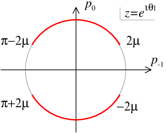
Figure 5: The bold line corresponds to the continuous spectrum of two-body states

As in $\phi^{4}$-interaction, the contribution from fig.(4)-(b) also violates the conservation of the three-momentum. We have computed the amplitude in the case that the external momenta are time-like. The result is

$$i\Gamma^{(2)}_{NP} = \frac{\pi}{\sqrt{1-m^{2}}}\theta(-p_{0}p^{\prime}_{0})\ \delta(p_{-1}-p^{\prime}_{-1})$$ (82)

$$\times\frac{1}{\sqrt{\frac{1}{4}(p+p^{\prime})^{2}-m^{2}p^{2}}}\ \frac{2(1-m^{2})p^{2}-\frac{1}{4}(p+p^{\prime})^{2}}{-(\frac{1}{4}(p+p^{\prime})^{2})^{2}-4(1-m^{2})(\frac{1}{4}(p+p^{\prime})^{2}-m^{2}p^{2})}$$

where $p_{m}=p(h_{1})_{m},\ p^{\prime}_{m}=p(h_{2})_{m}$. This amplitude has the same problems discussed for the non-planar diagram from $\phi^{4}$-interaction.

4.4 Some comments on higher loops and renormalization

In the preceding subsections, we see that the one-loop contributions to the two-point function conserve $p^{2}$ while they do not conserve $p_{\mu}$. In higher loops, the $p^{2}$ is not conserved either. To see this, let us consider the diagram of fig.(4.4) as an example. The amplitude is proportional to

$$\int d\mu(g_{1})d\mu(g_{2})d\mu(g_{3})\delta(g_{1}g_{2}^{-1}h_{2}h_{1})\delta(g_{1}^{-1}g_{3}g_{2}g_{3})\sim\int d\mu(g_{1})d\mu(g_{3})\delta(g_{1}g_{3}^{-1}g_{1}^{-1}g_{3}h_{2}h_{1}).$$ (83)

Thus $h_{1}$ and $h_{2}$ do not need to belong to the same conjugacy class, and therefore $p^{2}$ is not conserved.

Figure 6: A $p^{2}$-violating graph

Figure 7: A divergent tadpole graph

Figure 8: A non-planar tadpole graph

As for the renormalization at one-loop order, the only divergent graphs are planar tadpole graphs such as fig.(4.4). These can be calculated simply by replacing the external momenta of the result of subsection 4.1. Then their external momentum dependence becomes $\delta(h_{1}\dots h_{n})$, and these divergences can be absorbed by $n$-point counter terms and renormalizable. No non-planar graphs such as fig.(4.4) diverge. This is because those graphs can be evaluated only by replacing the external momenta $(h_{1},h_{2})$ of the result of subsection 4.2 with those of appropriate channel $(h_{1}\dots h_{k},h_{k+1}\dots h_{n})$. Notice that the group manifold $\delta$-function at the vertex reduces the dimensions of loop-momentum integration and has an effect similar to the Moyal phase factor which serves as a damping factor. For example, in the non-planar graphs such as figs.(3) and (4.4), the loop momentum runs only over the one-dimensional subgroup of $SL(2,R)$ determined from the external momenta.

Beyond the one-loop order, we do not know whether the noncommutative scalar field theory we are discussing is renormalizable or not. In the case of scalar field theory with the Moyal type noncommutativity, renormalizability is shown up to two-loop [37] and also a convergence theorem of Feynman integral has recently been well understood [19]. For the noncommutative YM and QED cases, renormalizability is shown up to one-loop [38]-[40], [9]. In order to investigate the issue in our field theory from perturbative analysis, we need first a systematic evaluation of Feynman integral as was done in [19]. In the present work, this is out of our scope.

5 Translational symmetry

In the previous section, we have shown that the contributions from the non-planar diagram violates the momentum conservation. This violation comes from the fact that the commutation relations of the coordinate operators (1) do not respect the naive translational invariance, $\hat{x}^{\mu}\rightarrow\hat{x}^{\mu}+v^{\mu}$ with a c-number vector $v^{\mu}$. Since the translational invariance is recovered in the commutation relations in the commutative limit $l_{P}\rightarrow 0$, one naively expects that the violation should vanish in this limit. But this naive expectation is not true as we saw for the non-planar one-loop results in the preceding section. Since this violation exists substantially in the low energy limit while the momentum conservation is one of the fundamental components in the present theoretical physics, we need an exact symmetry in the noncommutative space-time, which corresponds to the translational symmetry in the commutative limit.

To introduce such symmetry, let us define a field

$$\hat{\Psi}=\sum_{n=0}\int d\mu(g)\ \Phi(g)_{\mu_{1}\cdots\mu_{n}}\ \hat{p}^{\mu_{1}}\cdots\hat{p}^{\mu_{n}}\exp(ik_{\mu}(g)\hat{x}^{\mu}),$$ (84)

where $\Phi(g)_{\mu_{1}\cdots\mu_{n}}$ are c-number tensor fields. This can be regarded as a non-local generalisation of the scalar field defined in (27).

Let us define a unitary operator

$$U(v)=\exp(iv_{\mu}\hat{p}^{\mu}).$$ (85)

The $p_{\mu}=0$ eigen-state $|0\rangle$ is invariant under this unitary operator

$$U|0\rangle=|0\rangle.$$ (86)

We define the translational transformation of the field $\hat{\Psi}$ by

$$\hat{\Psi}\rightarrow U^{\dagger}\hat{\Psi}U.$$ (87)

Then this translational transformation is a symmetry of the following type of action

$$S=\sum\langle 0|(\hat{\Psi}^{\dagger})^{m}f(\hat{p})\hat{\Psi}^{n}|0\rangle.$$ (88)

In usual commutative cases, the translational transformation just generates a phase shift $\exp(-ik_{\mu}v^{\mu})$, and the tensor fields $\hat{\Phi}(g)_{\mu_{1}\cdots\mu_{n}}$ do not mix. Hence we may truncate the fields only to the scalar sector. However, in our noncommutative case, since the commutation relations are given by (1), the tensor fields mix. Thus the translational symmetry transforms local fields into non-local ones in general.

This coordinate dependence of locality would not be ridiculous when we recall the initial motivation of considering the noncommutative space-time. One of the authors regarded the noncommutative space-time (1) as a space-time realizing a space-time uncertainty relation derived from a gedanken experiment [29]. We have no means to obtain a coordinate system more accurate than the limit specified by the space-time uncertainty relation. The uncertainty will become larger if a space-time event is farther from the origin of the coordinate system. Thus the space-time spread of an event is not an invariant notion anymore under the translational symmetry.

In places where the general relativity and quantum mechanics play major roles simultaneously, similar kinds of issues have already been observed in the literatures. The subtlety of the locality of an event has appeared already as an aspect of the black hole complementarity of Susskind [41]. For instance, he argued that the location of the baryon violation in a black hole geometry is an observer dependent notion. Moreover, in the holographic description of the world [42, 43], a space-time event is mapped to a screen, and the spread of the image will depend on the relative locations of the event and the screen [41].

Lastly we see that the action (88) may be derivable from a pregeometric action in the form

$$S_{preg}=\langle 0|g(\hat{\Psi}^{\dagger},\hat{\Psi})|0\rangle.$$ (89)

An action with a kinetic term would be generated in a certain background of the field $\hat{\Psi}=\hat{\Psi}_{0}$. For example, starting from a cubic pregeometric action and considering the background of $\hat{\Psi}_{0}$ with $\Phi_{0}=m^{2}$ and $\Phi_{0}^{\mu\nu}=\eta^{\mu\nu}$, we obtain an action with a kinetic term and cubic interactions for the fluctuation field $\hat{\Psi}_{1}$ in $\hat{\Psi}=\hat{\Psi}_{0}+\hat{\Psi}_{1}$. The action (89) would be more interesting than (88), since it has more symmetry.

6 Thermodynamics

In this section, we will discuss an analogue of thermodynamics of free scalar field theory in the noncommutative space-time. Reflecting the noncommutativity of the space-time, we find a non-trivial behaviour at high temperature. Following the common trick in usual commutative field theories, we will take the Euclidean metric and calculate the partition function, imposing the periodicity of the inverse temperature in the time-direction.

In the Euclidean metric with signature $\eta^{\mu\nu}=(1,1,1)$ , the consistency with the Jacobi identity changes the last commutation relation of (1) to

$$[\hat{p}^{\mu},\hat{x}^{\nu}]=-i\eta^{\mu\nu}\sqrt{1-l_{P}^{2}\hat{p}^{2}}+il_{P}\epsilon^{\mu\nu\rho}\hat{p}_{\rho}.$$ (90)

Thus the coordinate operators in the momentum representation are given by

$$\hat{x}^{\mu}=i\sqrt{1-l_{P}^{2}p^{2}}\frac{\partial}{\partial p_{\mu}}-il_{P}\epsilon^{\mu\nu\rho}p_{\nu}\frac{\partial}{\partial p^{\rho}},$$ (91)

where we have ignored the possible ambiguity [29].

We now use a parameterisation

$$p_{0} = \frac{1}{l_{P}}\cos\omega\sin\theta,$$ (92)

$$p_{1} = \frac{1}{l_{P}}\sin\omega\cos\varphi,$$ (93)

$$p_{2} = \frac{1}{l_{P}}\sin\omega\sin\varphi,$$ (94)

where the ranges of the parameters are given by

$$0\leq\theta<2\pi,\ 0\leq\omega\leq\frac{\pi}{2},\ 0\leq\varphi<2\pi.$$ (95)

Then the measure is given by

$$(1-l_{P}^{2}p^{2})^{-\frac{1}{2}}d^{3}p=d\theta d\omega d\varphi\sin\omega\cos\omega.$$ (96)

Using this parameterisation, the coordinate operators are rewritten as

$$x^{0} = il_{P}\left(\frac{\partial}{\partial\theta}-\frac{\partial}{\partial\varphi}\right),$$ (97)

$$x^{1} = il_{P}\left(\tan\omega\sin(\theta-\varphi)\frac{\partial}{\partial\theta}+\cos(\theta-\varphi)\frac{\partial}{\partial\omega}-\cot\omega\sin(\theta-\varphi)\frac{\partial}{\partial\varphi}\right),$$ (98)

$$x^{2} = il_{P}\left(\tan\omega\cos(\theta-\varphi)\frac{\partial}{\partial\theta}+\sin(\varphi-\theta)\frac{\partial}{\partial\omega}+\cot\omega\cos(\theta-\varphi)\frac{\partial}{\partial\varphi}\right).$$ (99)

Because of the noncommutativity of the coordinate operators, it is impossible to find an operator which shifts $x^{0}$ by a certain c-number while $x^{1,2}$ remain intact. Below we shall just find an operator which shifts $x^{0}$ by $\beta$ but does not change the expectation values $\langle\phi|x^{1,2}|\phi\rangle$, where $|\phi\rangle$ is an eigen-state of $x^{0}$.

From (99), we see that the eigen-function of the operator $x^{0}$ is given by

$$\phi=e^{id(\theta-\varphi)}f(\theta+\varphi,\omega).$$ (100)

The periodicities of the wave function under $\theta\rightarrow\theta+2\pi,\ \varphi\rightarrow\varphi+2\pi$ constrain the values of $d$ as

$$d=\frac{n_{d}}{2},$$ (101)

where $n_{d}$ is an integer, and leads to that $f$ must satisfy

$$f(y,\omega)=(-1)^{n_{d}}f(y+2\pi,\omega).$$ (102)

A candidate of the shift operator with $U^{\dagger}x^{0}U=x^{0}+\beta$ is given by

$$U(\beta)=\exp\left(-\frac{i}{l_{P}}\beta\theta\right),$$ (103)

where, in order to satisfy the periodicity with respect to $\theta$,

$$\beta=l_{P}n_{\beta}$$ (104)

with a positive integer $n_{\beta}$. Since $U^{\dagger}x^{1}U=x^{1}+\beta\tan\omega\sin(\theta-\varphi)$, we find

$$\langle\phi|\delta x^{1}|\phi\rangle = \langle\phi|(U^{\dagger}x^{1}U-x^{1})|\phi\rangle$$ (105)

$$= \beta\int d\theta d\omega d\varphi\sin\omega\cos\omega|f(\theta+\varphi,\omega)|^{2}\tan\omega\sin(\theta-\varphi)$$ (106)

$$= 0.$$ (107)

Similarly $\langle\phi|\delta x^{2}|\phi\rangle=0$. The shift operator $U$ could contain $\varphi$-derivative in order to satisfy only the above features. However, since $\varphi$-derivative generates a spatial rotation which we do not need, we assume that (103) is the appropriate operator.

The thermodynamic partition function for the inverse temperature $\beta$ is obtained by taking the trace with respect to the states satisfying $U|\phi\rangle=|\phi\rangle$. Hence we sum up over the states with $\theta=2\pi l_{P}n/\beta$, where $n$ is an arbitrary integer. Thus we obtain

$$\ln Z = -\frac{1}{2}{\rm Tr}_{U=1}\left(\ln(p^{2}+m^{2})\right)$$ (108)

$$= -\frac{1}{8\pi}\sum_{n=-\infty}^{\infty}\int d\theta d^{2}q\ \delta\left(\theta-\frac{2\pi l_{P}n}{\beta}\right)\ln\left(\frac{1}{l_{P}^{2}}\sin^{2}\theta+q^{2}\cos^{2}\theta+m^{2}\right).$$ (109)

The overall numerical constant is determined by comparing with the usual commutative case in the limit $\beta\rightarrow\infty$. The integration over $\theta$ can be done by the contour integration with the new variable $z=e^{i\theta}$ after applying the formula $\sum_{m}e^{2\pi mti}=\sum_{n}\delta(t-n)$ to (109). The result is

$$\ln Z = -\frac{1}{2\pi}\int_{0}^{\frac{1}{l_{P}}}qdq\ln\left(y_{+}^{\beta/2l_{P}}-y_{+}^{-\beta/2l_{P}}\right),$$ (110)

$$y_{+} = \sqrt{1+\frac{-q^{2}+1/l_{P}^{2}}{q^{2}+m^{2}}}+\sqrt{\frac{-q^{2}+1/l_{P}^{2}}{q^{2}+m^{2}}}.$$ (111)

The logarithm of the partition function (111) has the usual behaviour $\sim-1/\beta^{2}$ in the low temperature. If we ignore the quantisation of $\beta$ (104), it has the behaviour $\sim-\log\beta$ at the high temperature $\beta\ll l_{P}$. This suggests the reduction of the degrees of freedom in the high energy region. If we can apply the usual first law of thermodynamics to this system, we obtain the entropy density $s\sim-\ln\beta$ and the energy density $e\sim 1/\beta$ at the high temperature $\beta\ll l_{P}$. Thus $s/\sqrt{e}$ decreases when the temperature increases. On the other hand, in the low temperature region, $s/\sqrt{e}\sim 1/\sqrt{\beta}$, and it increases with the temperature. Thus there is an upper bound of $s/\sqrt{e}$, in agreement with the qualitative argument given in [32].

However, it is not clear whether we can really regard $\beta$ as the inverse of the temperature, and can use the first law of thermodynamics to obtain the energy and entropy. To have a reliable discussion on these issues, we have to construct statistical thermodynamics in the noncommutative space-time. To do so, we need a Hamiltonian and its spectra. Moreover, in usual commutative cases, a thermodynamic system is put in an imaginary box and the states are well regularized by the infrared cut-off given by the size of the box. Since these issues are non-trivial in the noncommutative space-time, the construction of statistical thermodynamics remains unsolved.

7 Summary and discussions

In this paper, we have analysed scalar field theories in the noncommutative three-dimensional space-time characterised by $[x^{\mu},x^{\nu}]=2il_{P}\epsilon^{\mu\nu\rho}x_{\rho}$. The one-particle Hilbert space in momentum representation is represented by the $SL(2,R)$ group manifold. Since momentums are elements of $SL(2,R)$, the interaction vertices have definite ordering of legs coming from the noncommutativity of the group elements. We have performed some one-loop computations, which can be evaluated explicitly by contour integrations in complex planes. The non-planar one-loop diagrams of the two-point functions from $\phi^{4}$ and $\phi^{3}$-interactions were shown to be finite and have the infrared singularity coming from the UV/IR mixing.

The most peculiar feature of the noncommutative space-time is that the commutation relations among the coordinates do not respect the translational symmetry. This violation of translational symmetry is natural from the view point of a fuzzy space-time [29]. If an event is farther from the origin of a reference frame, the location of the event will become more fuzzy by the quantum fluctuation of the space-time. Since the translational symmetry is recovered in the $l_{P}\rightarrow 0$ limit in the commutation relations (1), one might expect that the momentum conservation would be recovered in this limit. However we have shown explicitly that this is not true for the non-planar contributions. To remedy this defect, we had to introduce an infinite number of tensor fields. We leave the analysis of the messy theory with an infinite number of tensor fields for future work.

On the other hand, the noncommutativity at the boundary of a membrane in the $C$-field background in M-theory is the loop-space noncommutativity $[x^{\mu}(\sigma),x^{\nu}(\sigma^{\prime})]\sim i\epsilon^{\mu\nu\rho}x_{\rho}^{\prime}(\sigma)\delta(\sigma-\sigma^{\prime})$ [26, 27]. This noncommutativity obviously respects the translational symmetry. Since the noncommutative string theory comes from a limit of M-theory, the theory might be controllable. Thus, concerning the interests in noncommutative field theories in more than two-dimensions, the noncommutative string theory might be interesting.

We have finally discussed an analogue of thermodynamics of noncommutative free scalar field theory. What we have computed is the partition function of free scalar field theory in a noncommutative three-dimensional space with Euclidean signature, following the common trick in usual commutative field theories. The result shows the reduction of the degrees of freedom in the ultraviolet, which comes essentially from the compactness of the momentum space in the case of Euclidean signature. However it is not clear to us whether the partition function is really related to the thermodynamics of the noncommutative field theory, since the noncommutativity of the time coordinate makes it hard to define statistical thermodynamics in a convincing way.

There seem to exist several puzzles on the three-dimensional noncommutative field theory such as unitarity and renormalizability. To analyse these issues perturbatively, we need to develop further the computational technic of $SL(2,R)$ group theoretic Feynman integral. We hope that the present work may be meaningful as a primitive step toward consistent treatment of quantum field theories in more than two-dimensional noncommutative space-times.

Acknowledgements
The authors would like to thank N. Ikeda for valuable discussions. N.S. is supported in part by Grant-in-Aid for Scientific Research (#12740150), and in part by Priority Area: “Supersymmetry and Unified Theory of Elementary Particles” (#707), from Ministry of Education, Science, Sports and Culture.

References

• [1] A. Connes, M.R. Douglas and A. Schwarz, JHEP 9802 (1998) 003, hep-th/9711162.
• [2] M.R. Douglas and C. Hull, JHEP 9802 (1998) 008, hep-th/9711165.
• [3] C.-S. Chu and P.-M. Ho, Nucl. Phys. B550 (1999) 151, hep-th/9812219; Nucl. Phys. B568 (2000) 447, hep-th/9906192.
• [4] V. Schomerus, JHEP 9906 (1999) 030, hep-th/9903205.
• [5] F. Ardalan, H. Arfaei and M.M. Sheikh-Jabbari, hep-th/9803067;JHEP 9902 (1999) 016, hep-th/9810072; Nucl. Phys. B576 (2000) 578, hep-th/9906161.
• [6] D. Bigatti and L. Susskind, hep-th/9908056.
• [7] N. Seiberg and E. Witten, JHEP 9909 (1999) 032, hep-th/9908142.
• [8] S. Minwalla, M.V. Raamsdonk and N. Seiberg, hep-th/9912072.
• [9] M. Hayakawa, Phys. Lett. B478 (2000) 394, hep-th/9912094; hep-th/9912167.
• [10] A. Matusis, L. Susskind and N. Toumbas, hep-th/0002075.
• [11] M.V. Raamsdonk and N. Seiberg, JHEP 0003 (2000) 035, hep-th/0002186.
• [12] W. Fischler, E. Gorbatov, A. Kashani-Poor, S. Paban, P. Pouliot and J. Gomis, JHEP 0005 (2000) 024, hep-th/0002067.
• [13] B.A. Campbell and K. Kaminsky, Nucl. Phys. B581 (2000) 240, hep-th/0003137.
• [14] W. Fischler, E. Gorbatov, A. Kashani-Poor, R. McNees, S. Paban and P. Pouliot, JHEP 0006 (2000) 032, hep-th/0003216.
• [15] N. Seiberg, L. Susskind and N. Toumbas, JHEP 0006 (2000) 044, hep-th/0005015.
• [16] R. Gopakumar, J. Maldacena, S. Minwalla and A. Strominger, JHEP 0006 (2000) 036, hep-th/0005048.
• [17] J.L.F. Barbon and E. Rabinovici, Phys. Lett. B486 (2000) 202, hep-th/0005073.
• [18] J. Gomis and T. Mehen, hep-th/0005129.
• [19] I. Chepelev and R. Roiban, JHEP 0005 (2000) 037, hep-th/9911098; hep-th/0008090
• [20] G. Arcioni and M.A. Vázquez-Mozo, JHEP 0001 (2000) 028 , hep-th/9912140.
• [21] G. Arcioni, J.L.F. Barbon, J. Gomis and M.A. Vázquez-Mozo, JHEP 0006 (2000) 038, hep-th/0004080.
• [22] E. Hawkins, Comm. Math. Phys. 202 (1999) 517-546, q-alg/9708030.
• [23] C. Klimcik, Comm. Math. Phys. 199 (1998) 257-279, hep-th/9710153.
• [24] U. C.-Watamura and S. Watamura, Comm. Math. Phys. 212 (2000) 395, hep-th/9801195.
• [25] J. Madore, S. Schraml, P. Schupp and J. Wess, hep-th/0001203.
• [26] E. Bergshoeff, D.S. Berman, J.P. van der Schaar, P. Sundell, hep-th/0005026.
• [27] S. Kawamoto and N. Sasakura, JHEP 0007 (2000) 014, hep-th/0005123.
• [28] P.-M. Ho and Y.-T. Yeh, hep-th/0005159.
• [29] N. Sasakura, JHEP 0005 (2000) 015, hep-th/0001161.
• [30] F. Karolyhazy, Nuovo Cim. A42 (1966) 390.
• [31] Y. J. Ng and H. van Dam, Mod. Phys. Lett. A9 (1994) 335; A10 (1995) 2801.
• [32] N. Sasakura, Prog. Theor. Phys. 102 (1999) 169, hep-th/9903146.
• [33] S. Doplicher, K. Fredenhagen and J.E. Roberts, Phys. Lett. B331 (1994) 39.
• [34] D.V. Ahluwalia, Phys. Lett. B339 (1994) 301.
• [35] See T. Yoneya, hep-th/0004074, as a recent review of the space-time uncertainty principle in string theory.
• [36] P. Kosinski, J. Lukierski and P. Maslanka, Phys. Rev. D62 (2000) 025004, hep-th/9902037.
• [37] A. Micu and M.M. Sheikh-Jabbari, hep-th/0008057.
• [38] C.P. Martin and D. Sanchez-Ruiz, Phys. Rev. Lett. 83 (1999) 476, hep-th/9903077.
• [39] M.M. Sheikh-Jabbari, JHEP 9906 (1999) 0157, hep-th/9903107.
• [40] T. Krajewski and R. Wulkenhaar, Int. J. Mod. Phys. A15 (2000) 1011, hep-th/9903187.
• [41] See as a review, D. Bigatti and L. Susskind, hep-th/0002044.
• [42] G. ’t Hooft, gr-qc/9310026.
• [43] L. Susskind, J. Math. Phys. 36 (1995) 6377.
• [44] H. Hata, K. Itoh, T. Kugo, H. Kunitomo and K. Ogawa, Phys. Lett. B175 (1986) 138.