UMTG–224

Exact solution of the supersymmetric sinh-Gordon model with boundary
Changrim Ahn and Rafael I. Nepomechie

The boundary supersymmetric sinh-Gordon model is an integrable quantum field theory in $1+1$ dimensions with bulk $N=1$ supersymmetry, whose bulk and boundary $S$ matrices are not diagonal. We present an exact solution of this model. In particular, we derive an exact inversion identity and the corresponding thermodynamic Bethe Ansatz equations. We also compute the boundary entropy, and find a rich pattern of boundary roaming trajectories corresponding to $c<3/2$ superconformal models.

1 Introduction

The supersymmetric sinh-Gordon (SShG) model [1]-[6] is one of the simplest examples of a $1+1$ dimensional integrable quantum field theory with $N=1$ supersymmetry. Indeed, the particle spectrum consists of one Boson and one Fermion which have equal mass and which enjoy factorized scattering [7]. As such, SShG is a valuable toy model.

In this article, we consider the boundary SShG model, with boundary conditions that preserve the bulk integrability, but not necessarily the bulk supersymmetry [8]-[11]. In addition to its usefulness as a simple prototype, we expect that this model may also have applications to quantum impurity problems [12].

An interesting feature of the boundary SShG model is that the $S$ matrices which have been conjectured for both bulk and boundary scattering are not diagonal. Our main objective is to perform a thermodynamic Bethe Ansatz (TBA) analysis [6], [13]-[17] for this model, using these conjectured $S$ matrices as inputs. Such analysis can provide checks on the input $S$ matrix data, as well as information about the underlying boundary conformal field theory [18]-[19].

Conventional wisdom suggests that the problem of determining the necessary Bethe Ansatz equations is intractable, due to the fact that the boundary $S$ matrix is not diagonal. Nevertheless, we succeed to determine the Bethe Ansatz equations and carry out the TBA analysis for the boundary SShG model. This is the first example of a model with non-diagonal boundary $S$ matrix which is exactly solved.

We also obtain an expression for the boundary entropy [20],[17] for the boundary SShG model. Moreover, we find a rich pattern of boundary roaming trajectories corresponding to $c<3/2$ superconformal models [21], [22], thereby generalizing previous work on bulk [23]-[25] and boundary [26], [27] roaming.

The outline of this article is as follows. In Sec. 2 we review the scattering theory of the boundary SShG model, which serves as our input. Here we also show that the strong-weak duality symmetry of the bulk model (see, e.g., [28]) extends also to the model with boundary. Moreover, we introduce the notations and conventions which are used throughout the paper. In Sec. 3 we formulate the so-called Yang matrix [29] and relate it to a commuting transfer matrix, which is the true starting point of any TBA analysis. For the problem at hand, we require a boundary version of the Yang matrix [30], [31], which presents an interesting complication with respect to the more familiar case of periodic boundary conditions. In Sec. 4 we use the open-chain fusion formula [32] to derive an exact inversion identity, using which we obtain the eigenvalues of the transfer matrix in terms of roots of certain Bethe Ansatz equations. That such an inversion identity exists is presumably due to the fact that the bulk $S$ matrix satisfies the so-called free Fermion condition [33], [34]. In Sec. 5 we use these results to derive the TBA equations. Certain remarkable identities lead to very simple formulas, in particular for the boundary entropy. In Sec. 6 we use our result for the boundary entropy to obtain boundary roaming trajectories. Finally, in Sec. 7 we discuss our results and describe some possible generalizations.

2 Review of boundary SShG scattering theory

In this Section, we review the bulk and boundary $S$ matrices which have been proposed for the boundary supersymmetric sinh-Gordon model. As mentioned in the Introduction, these $S$ matrices will be used as inputs in the calculations that follow. We also show that the strong-weak duality symmetry of the bulk model extends also to the model with boundary.

2.1 Bulk

In order to understand the SShG scattering theory, it is essential to first consider a related model, namely, the supersymmetric sine-Gordon (SSG) model, whose Euclidean-space Lagrangian density is given by

$${\cal L}^{SSG}_{bulk}={1\over 2}\left(\partial_{z}\phi\partial_{\bar{z}}\phi+\bar{\psi}\partial_{z}\bar{\psi}+\psi\partial_{\bar{z}}\psi\right)+iM\bar{\psi}\psi\cos\beta\phi+{M^{2}\over 2\beta^{2}}\sin^{2}\beta\phi\,,$$ (2.1)

where $\phi(z\,,\bar{z})$ is a real scalar field, $\psi(z\,,\bar{z})$ and $\bar{\psi}(z\,,\bar{z})$ are the components of a Majorana spinor field, and $\beta$ is the dimensionless coupling constant. The Lagrangian density for the supersymmetric sinh-Gordon (SShG) model is obtained by analytic continuation to imaginary coupling, i.e. setting $\beta=i\hat{\beta}$ with $\hat{\beta}$ real:

$${\cal L}^{SShG}_{bulk}={1\over 2}\left(\partial_{z}\phi\partial_{\bar{z}}\phi+\bar{\psi}\partial_{z}\bar{\psi}+\psi\partial_{\bar{z}}\psi\right)+iM\bar{\psi}\psi\cosh\hat{\beta}\phi+{M^{2}\over 2\hat{\beta}^{2}}\sinh^{2}\hat{\beta}\phi\,.$$ (2.2)

Both of these models have $N=1$ supersymmetry (without topological charge) [1], [2] and are integrable [3], [4].

Observe that SSG has a periodic potential, which admits classical soliton solutions that interpolate between neighboring minima. Correspondingly, it has been proposed [35]-[37] that the SSG quantum spectrum consists of supersymmetric multiplets of kinks of mass $m$ and breathers (bound states of kinks) of mass $m_{n}=2m\sin(n\alpha\pi)$, $n=1\,,2\,,\ldots\,,[{1\over 2\alpha}]$, where

$$\alpha={{\beta^{2}\over 4\pi}\over 1-{\beta^{2}\over 4\pi}}\,,$$ (2.3)

and $[x]$ denotes integer part of $x$. Hence, breathers can be present only if $0<\alpha<{1\over 2}$. The lightest ($n=1$) breathers are identified as the elementary particles (Boson, Fermion) corresponding to the fields in the Lagrangian density (2.1).

Upon making the analytic continuation to SShG (which is the model of primary interest), we see that the potential is no longer periodic, and hence, there are no longer any classical soliton solutions. Thus, the SShG quantum spectrum does not contain kinks; it consists only of the elementary particles of some mass $m$ corresponding to the fields in the Lagrangian density (2.2), i.e. corresponding to the $n=1$ SSG breather. Setting $\beta=i\hat{\beta}$ in Eq. (2.3), we obtain

$$\alpha=-{{\hat{\beta}^{2}\over 4\pi}\over 1+{\hat{\beta}^{2}\over 4\pi}}\equiv-B\,,$$ (2.4)

where we have introduced the SShG parameter $B$.

Since the SShG spectrum corresponds to the $n=1$ SSG breather, we infer that the SShG $S$ matrix $S(\theta)$ for two particles of rapidities $\theta_{1}\,,\theta_{2}$ (and corresponding energy $E_{i}=m\cosh\theta_{i}$ and momentum $P_{i}=m\sinh\theta_{i}$, $i=1\,,2$) is given by the analytic continuation of the $n=1$ SSG breather $S$ matrix,

$$S(\theta)=S_{ShG}(\theta)\ S_{SUSY}(\theta)\,,$$ (2.5)

where $\theta=\theta_{1}-\theta_{2}$. The scalar factor $S_{ShG}(\theta)$ is given by

$$S_{ShG}(\theta)={\sinh\theta-i\sin(2B\pi)\over\sinh\theta+i\sin(2B\pi)}\,.$$ (2.6)

This is the $S$ matrix of the usual (non-supersymmetric) sinh-Gordon model [38],[39], which is the analytic continuation of the $n=1$ SG breather $S$ matrix [40], but with a different dependence on the coupling constant. It satisfies

$$S_{ShG}(\theta)\ S_{ShG}(-\theta)=1\,,\qquad S_{ShG}(\theta)=S_{ShG}(i\pi-\theta)\,.$$ (2.7)

The factor $S_{SUSY}(\theta)$ is given by

$$S_{SUSY}(\theta)=Y(\theta)\ R(\theta)\,,$$ (2.8)

where $R(\theta)$ is a $4\times 4$ matrix acting on the tensor product space $V\otimes V$, where $V$ is the 2-dimensional vector space of 1-particle states. We choose $\{|b(\theta)\rangle\,,|f(\theta)\rangle\}$ to be the basis of $V$ (corresponding to a Boson, Fermion with rapidity $\theta$, respectively); and hence, the basis of $V\otimes V$ is given by $\{|b_{1}\,,b_{2}\rangle\,,|b_{1}\,,f_{2}\rangle\,,|f_{1}\,,b_{2}\rangle\,,|f_{1}\,,f_{2}\rangle\}$, where $|b_{1}\,,b_{2}\rangle\equiv|b(\theta_{1})\,,b(\theta_{2})\rangle$ , etc. In this basis, $R(\theta)$ is given by

$$R(\theta)=\left(\begin{array}[]{cccc}a_{+}(\theta)&0&0&d(\theta)\\ 0&b&c(\theta)&0\\ 0&c(\theta)&b&0\\ d(\theta)&0&0&a_{-}(\theta)\end{array}\right)\,,$$ (2.13)

with

$$a_{\pm}(\theta)=\pm 1-{2i\sin B\pi\over\sinh\theta}\,,\qquad b=1\,,\qquad c=-{i\sin B\pi\over\sinh{\theta\over 2}}\,,\qquad d=-{\sin B\pi\over\cosh{\theta\over 2}}\,.$$ (2.14)

It is important to note that the matrix elements of $R(\theta)$ satisfy the “free Fermion” condition [33], [6]

$$a_{+}a_{-}+b^{2}=c^{2}+d^{2}\,.$$ (2.15)

The matrix $R(\theta)$ is a solution of the Yang-Baxter equation

$$R_{12}(\theta_{1}-\theta_{2})\ R_{13}(\theta_{1}-\theta_{3})\ R_{23}(\theta_{2}-\theta_{3})\ =R_{23}(\theta_{2}-\theta_{3})\ R_{13}(\theta_{1}-\theta_{3})\ R_{12}(\theta_{1}-\theta_{2})\,.$$ (2.16)

This matrix is both $\sf P$ and $\sf T$ invariant,

$${\cal P}_{12}\ R_{12}(\theta)\ {\cal P}_{12}=R_{12}(\theta)\,,\qquad R_{12}(\theta)^{t_{1}t_{2}}=R_{12}(\theta)\,,$$ (2.17)

where $t_{i}$ denotes transposition in the $i^{th}$ space, and ${\cal P}$ is the permutation matrix

$${\cal P}=\left(\begin{array}[]{cccc}1&0&0&0\\ 0&0&1&0\\ 0&1&0&0\\ 0&0&0&1\end{array}\right)\,.$$ (2.22)

Moreover, $Y(\theta)$ is a scalar factor given by

$$Y(\theta)={\sinh{\theta\over 2}\over\sinh{\theta\over 2}-i\sin B\pi}\exp\left(-\int_{0}^{\infty}{dt\over t}\ {\sinh(it\theta/\pi)\sinh(t(1+B))\sinh(tB)\over\cosh t\cosh^{2}{t\over 2}}\right)\,,$$ (2.23)

which is a solution of the unitarity and crossing constraints

$$Y(\theta)\ Y(-\theta)={\sinh^{2}{\theta\over 2}\over\sinh^{2}{\theta\over 2}+\sin^{2}B\pi}\,,\qquad Y(\theta)=Y(i\pi-\theta)\,.$$ (2.24)

Let us denote the total scalar factor by $Z(\theta)$

$$Z(\theta)=S_{ShG}(\theta)\ Y(\theta)\,.$$ (2.25)

One can show that $Z(\theta)$ has the integral representation [6]

$$Z(\theta)={\sinh{\theta\over 2}\over\sinh{\theta\over 2}+i\sin B\pi}\exp\left(\int_{0}^{\infty}{dt\over t}\ {\sinh(it\theta/\pi)\sinh(t(1-B))\sinh(tB)\over\cosh t\cosh^{2}{t\over 2}}\right)\,,$$ (2.26)

which is the same as the expression in Eq. (2.23), except with $B\rightarrow-B$. It has no poles in the physical strip ($0<Im\ \theta<\pi$), provided $B$ lies in the range

$$0<B<1\,,$$ (2.27)

which corresponds to $0<\hat{\beta}^{2}<\infty$.

In short, the proposed SShG bulk $S$ matrix $S(\theta)$ is given by

$$S(\theta)=Z(\theta)\ R(\theta)\,,$$ (2.28)

where the scalar factor $Z(\theta)$ is given by Eq. (2.26) and the matrix $R(\theta)$ is given by Eqs. (2.13), (2.14).

It is known (see, e.g., [28]) that the SShG bulk $S$ matrix is invariant under the strong-weak duality transformation $\hat{\beta}\rightarrow 4\pi/\hat{\beta}$, which implies

$$B\rightarrow 1-B\,.$$ (2.29)

Indeed, this invariance can be checked by inspection of the matrix elements (2.14) of $R(\theta)$ and the expression (2.26) for $Z(\theta)$. (The factors $S_{ShG}(\theta)$ and $Y(\theta)$ are not separately invariant.) Note that this transformation maps the range (2.27) into itself.

2.2 Boundary

We turn now to boundary conditions and boundary scattering, following the framework developed by Ghoshal and Zamolodchikov [8]. An investigation of which boundary terms can be added to the bulk SShG model (2.2) without spoiling (classical) integrability has led to the following results [9]: the boundary Lagrangian

$$L^{SShG}_{boundary}=\Lambda\cosh\hat{\beta}(\phi-\phi_{0})+\mathsf{M}\bar{\psi}\psi+\epsilon\psi+\bar{\epsilon}\bar{\psi}\,,\qquad\mathsf{M}\neq\pm 1\,,$$ (2.30)

breaks supersymmetry but preserves integrability; and

$$L^{SShG}_{boundary}=\mp{M\over\hat{\beta}^{2}}\cosh\hat{\beta}\phi\pm\bar{\psi}\psi$$ (2.31)

preserves both supersymmetry and integrability. Notice that the boundary terms (2.30) involve a total of 5 boundary parameters $\Lambda\,,\phi_{0}\,,\mathsf{M}\,,\epsilon\,,\bar{\epsilon}$. If $\epsilon\,,\bar{\epsilon}$ are nonzero, then Fermion number is not conserved.

The proposed boundary $S$ matrix $\mathsf{S}(\theta)$ for a particle of rapidity $\theta$ is given by (compare with Eq. (2.5)) ,

$$\mathsf{S}(\theta)=\mathsf{S}_{ShG}(\theta\,;\eta\,,\vartheta)\ \mathsf{S}_{SUSY}^{(\varepsilon)}(\theta\,;\varphi)\,.$$ (2.32)

The scalar factor $\mathsf{S}_{ShG}(\theta\,;\eta\,,\vartheta)$, which depends on two boundary parameters $\eta\,,\vartheta$, is given by

$$\mathsf{S}_{ShG}(\theta\,;\eta\,,\vartheta)=\mathsf{X}_{0}(\theta)\ \mathsf{X}_{1}(\theta\,;{4\eta B\over\pi})\ \mathsf{X}_{1}(\theta\,;{4i\vartheta B\over\pi})\,,$$ (2.33)

where

$$\mathsf{X}_{0}(\theta)=(1)(1+2B)(2-2B)\,,\qquad\mathsf{X}_{1}(\theta\,;F)={1\over(1-F)(1+F)}\,,$$ (2.34)

with

$$(x)\equiv{\sinh({\theta\over 2}+{i\pi x\over 4})\over\sinh({\theta\over 2}-{i\pi x\over 4})}\,.$$ (2.35)

This is the boundary $S$ matrix of the usual (non-supersymmetric) boundary sinh-Gordon model, which is the analytic continuation of the $n=1$ boundary sine-Gordon breather $S$ matrix [44]. It satisfies

$$\mathsf{S}_{ShG}(\theta\,;\eta\,,\vartheta)\ \mathsf{S}_{ShG}(-\theta\,;\eta\,,\vartheta)=1\,,\quad\mathsf{S}_{ShG}({i\pi\over 2}+\theta\,;\eta\,,\vartheta)\ S_{ShG}(2\theta)\ =\mathsf{S}_{ShG}({i\pi\over 2}-\theta\,;\eta\,,\vartheta)\,.$$

(2.36)

The factor $\mathsf{S}_{SUSY}^{(\varepsilon)}(\theta\,;\varphi)$ is given by [10]

$$\mathsf{S}_{SUSY}^{(\varepsilon)}(\theta\,;\varphi)=\mathsf{Y}^{(\varepsilon)}(\theta\,;\varphi)\ \mathsf{R}^{(\varepsilon)}(\theta\,;\varphi)\,,$$ (2.37)

where $\varepsilon$ is a discrete parameter which can be either $+1$ or $-1$, and $\varphi$ is a continuous boundary parameter. $\mathsf{R}^{(\varepsilon)}(\theta\,;\varphi)$ is a $2\times 2$ matrix acting on the vector space $V$ of 1-particle states, which is given by

$$\mathsf{R}^{(\varepsilon)}(\theta\,;\varphi)=\left(\begin{array}[]{cc}\cosh{\theta\over 2}\ G_{+}^{(\varepsilon)}+i\sinh{\theta\over 2}\ G_{-}^{(\varepsilon)}&-\varepsilon i\sinh\theta\\ -i\sinh\theta&\cosh{\theta\over 2}\ G_{+}^{(\varepsilon)}-i\sinh{\theta\over 2}\ G_{-}^{(\varepsilon)}\end{array}\right)\,,$$ (2.40)

where

$$G_{\varepsilon^{\prime}}^{(\varepsilon)}=\left\{\begin{array}[]{r@{\quad\mbox{if} \quad}l}r\left(\cosh\varphi+e^{\varepsilon\varphi}{\sinh^{2}{\theta\over 2}\over 1+\varepsilon\sin B\pi}\right)&\varepsilon^{\prime}=\varepsilon\\ r\left(\sinh\varphi+\varepsilon e^{\varepsilon\varphi}{\sinh^{2}{\theta\over 2}\over 1+\varepsilon\sin B\pi}\right)&\varepsilon^{\prime}=-\varepsilon\end{array}\right.\,,$$ (2.43)

and

$$r=\left({2(\varepsilon+\sin B\pi)\over\sin B\pi}\right)^{1\over 2}\,.$$ (2.44)

The matrix $\mathsf{R}^{(\varepsilon)}(\theta\,;\varphi)$ is a solution of the boundary Yang-Baxter equation [45]

$$R_{12}(\theta_{1}-\theta_{2})\ \mathsf{R}_{1}^{(\varepsilon)}(\theta_{1}\,;\varphi)\ R_{12}(\theta_{1}+\theta_{2})\ \mathsf{R}_{2}^{(\varepsilon)}(\theta_{2}\,;\varphi)$$ (2.45)

$$=\mathsf{R}_{2}^{(\varepsilon)}(\theta_{2}\,;\varphi)\ R_{12}(\theta_{1}+\theta_{2})\ \mathsf{R}_{1}^{(\varepsilon)}(\theta_{1}\,;\varphi)\ R_{12}(\theta_{1}-\theta_{2})\,.$$

We remark that for $\varphi\rightarrow\pm\infty$, the matrix $\mathsf{R}^{(\varepsilon)}(\theta\,;\varphi)$ becomes diagonal and commutes with linear combinations $Q\pm\bar{Q}$ of the supersymmetry charges [10],[11].

In order to determine the scalar factor $\mathsf{Y}^{(\varepsilon)}(\theta\,;\varphi)$, we recall that the full boundary $S$ matrix must satisfy boundary unitarity $\mathsf{S}(\theta)\ \mathsf{S}(-\theta)=\mathbb{I}$ and boundary cross-unitarity [8], which can be written in matrix form as

$$\mathop{\rm tr}\nolimits_{0}\mathsf{S}_{0}({i\pi\over 2}+\theta)^{t_{0}}\ {\cal P}_{01}\ S_{01}(2\theta)^{t_{1}}=\mathsf{S}_{1}({i\pi\over 2}-\theta)\,.$$ (2.46)

We observe that the matrix $\mathsf{R}^{(\varepsilon)}(\theta\,;\varphi)$ satisfies

$$\mathsf{R}^{(\varepsilon)}(\theta\,;\varphi)\ \mathsf{R}^{(\varepsilon)}(-\theta\,;\varphi)=h(\theta)\ \mathbb{I}\,,$$ (2.47)

where

$$h(\theta)=\left(c_{0}+c_{1}\sinh^{2}{\theta\over 2}+c_{2}\sinh^{4}{\theta\over 2}\right)\cosh\theta\,,$$ (2.48)

and

$$c_{0}=\left\{\begin{array}[]{cc}r^{2}\cosh^{2}\varphi&\mbox{ if }\varepsilon=+1\\ r^{2}\sinh^{2}\varphi&\mbox{ if }\varepsilon=-1\end{array}\right.\,,\quad c_{1}={r^{2}e^{\varepsilon 2\varphi}\over 1+\varepsilon\sin B\pi}+2\varepsilon\,,\quad c_{2}={r^{2}e^{\varepsilon 2\varphi}\over(1+\varepsilon\sin B\pi)^{2}}\,.$$ (2.51)

Also,

$$\mathop{\rm tr}\nolimits_{0}\mathsf{R}^{(\varepsilon)}_{0}({i\pi\over 2}+\theta\,;\varphi)^{t_{0}}\ {\cal P}_{01}\ R_{01}(2\theta)^{t_{1}}=g(\theta)\ \mathsf{R}^{(\varepsilon)}_{1}({i\pi\over 2}-\theta\,;\varphi)\,,$$ (2.52)

where

$$g(\theta)={\varepsilon\sinh\theta-i\sin\pi B\over\sinh\theta}\,.$$ (2.53)

Setting

$$\mathsf{Y}^{(\varepsilon)}(\theta\,;\varphi)=\mathsf{Y}_{0}^{(\varepsilon)}(\theta)\ \mathsf{Y}_{1}^{(\varepsilon)}(\theta\,;\varphi)\,,$$ (2.54)

it follows that $\mathsf{Y}_{0}^{(\varepsilon)}(\theta)$ and $\mathsf{Y}_{1}^{(\varepsilon)}(\theta\,;\varphi)$ must satisfy

$$\mathsf{Y}_{0}^{(\varepsilon)}(\theta)\ \mathsf{Y}_{0}^{(\varepsilon)}(-\theta)\ \cosh\theta=1\,,\qquad\mathsf{Y}_{0}^{(\varepsilon)}({i\pi\over 2}+\theta)\ Y(2\theta)\ g(\theta)=\mathsf{Y}_{0}^{(\varepsilon)}({i\pi\over 2}-\theta)\,,$$ (2.55)

and

$$\mathsf{Y}_{1}^{(\varepsilon)}(\theta\,;\varphi)\mathsf{Y}_{1}^{(\varepsilon)}(-\theta\,;\varphi)\left(c_{0}+c_{1}\sinh^{2}{\theta\over 2}+c_{2}\sinh^{4}{\theta\over 2}\right)=1\,,\quad\mathsf{Y}_{1}^{(\varepsilon)}({i\pi\over 2}+\theta\,;\varphi)=\mathsf{Y}_{1}^{(\varepsilon)}({i\pi\over 2}-\theta\,;\varphi)\,,$$

(2.56)

respectively.

For simplicity, we shall henceforth restrict our attention to the case $\varepsilon=+1$, and so we shall drop the superscript $(\varepsilon)$. We propose the following integral representations for $\mathsf{Y}_{0}(\theta)$ and $\mathsf{Y}_{1}(\theta\,;\varphi)$:

$$\mathsf{Y}_{0}(\theta) = {i\over\sqrt{2}\sinh({\theta\over 2}+{i\pi\over 4})}\exp\left({1\over 2}\int_{0}^{\infty}{dt\over t}\ {\sinh(2it\theta/\pi)\sinh(t(1+B))\sinh(tB)\over\cosh^{2}t\cosh^{2}{t\over 2}}\right)\,,$$

$$\mathsf{Y}_{1}(\theta\,;\varphi) = {1\over r\cosh\varphi}\exp\left(4\int_{0}^{\infty}{dt\over t}\ {\cosh(t\zeta/\pi)\cosh({t\over 2}(1-2B))\sinh({t\over 2}(1+{i\theta\over\pi}))\sinh({it\theta\over 2\pi})\over\sinh t\cosh{t\over 2}}\right)\,,$$

where $\zeta$ is a function of the boundary parameter $\varphi$ defined by

$$\zeta=\cos^{-1}\left(1+e^{-2\varphi}(1+\sin B\pi)\right)\,.$$ (2.58)

In order to streamline the notation, let us denote the set of boundary parameters $\{\eta\,,\vartheta\,,\varphi\}$ by $\xi$, and denote the total scalar factor by $\mathsf{Z}(\theta\,;\xi)$

$$\mathsf{Z}(\theta\,;\xi) = \mathsf{S}_{ShG}(\theta\,;\eta\,,\vartheta)\ \mathsf{Y}(\theta\,;\varphi)$$ (2.59)

$$= \mathsf{Z}_{0}(\theta)\ \mathsf{Z}_{1}(\theta\,;\xi)\,.$$

The proposed SShG boundary $S$ matrix is then given by

$$\mathsf{S}(\theta\,;\xi)=\mathsf{Z}(\theta\,;\xi)\ \mathsf{R}(\theta\,;\varphi)\,.$$ (2.60)

We now observe that the boundary $S$ matrix is also invariant under the strong-weak duality transformation (2.29). Indeed, it is evident that the matrix $\mathsf{R}(\theta\,;\varphi)$ (2.40) has this invariance, if we assume that the parameter $\varphi$ remains invariant under this transformation. Let us now consider the scalar factor. The part of the scalar factor that does not depend on boundary parameters can be written in the form

$$\mathsf{Z}_{0}(\theta) = \mathsf{X}_{0}(\theta)\ \mathsf{Y}_{0}(\theta)$$

$$= {i\over\sqrt{2}\sinh({\theta\over 2}-{i\pi\over 4})}$$

$$\times \exp\left(-{1\over 4}\int_{0}^{\infty}{dt\over t}\ {\sinh(2it\theta/\pi)\over\cosh^{2}t\cosh^{2}{t\over 2}}\left[\cosh(t(1-2B))(1+2\cosh t)+\cosh t\right]\right)\,,$$ (2.62)

in which the duality invariance is manifest. (The factors $\mathsf{X}_{0}(\theta)$ and $\mathsf{Y}_{0}(\theta)$ are not separately invariant.) Finally, the part of the scalar factor which does depend on boundary parameters,

$$\mathsf{Z}_{1}(\theta\,;\xi)=\mathsf{X}_{1}(\theta\,;{4\eta B\over\pi})\ \mathsf{X}_{1}(\theta\,;{4i\vartheta B\over\pi})\ \mathsf{Y}_{1}(\theta\,;\varphi)\,,$$ (2.63)

is also invariant under duality, since each of its factors are separately invariant (provided the boundary parameters $\eta B$ and $\vartheta B$ are assumed to remain invariant).

3 Yang equations

Having specified the bulk and boundary $S$ matrices, we are ready to start the TBA program. The first step is to formulate the Yang matrix and relate it to a commuting transfer matrix. Since this is not obvious for the case of boundaries, we begin by reviewing the more familiar case of periodic boundary conditions.

3.1 Closed

We consider $N$ particles of mass $m$ with real rapidities $\theta_{1}\,,\ldots\,,\theta_{N}$ and two-particle $S$ matrix $S(\theta)$ (2.28) in a periodic box of length $L>>{1\over m}$. The Yang equation [29], [16] for particle 1 (which has momentum $P_{1}=m\sinh\theta_{1}$) is given by

$$\left(e^{iLm\sinh\theta_{1}}Y_{(1)}-\mathbb{I}\right)|\theta_{1}\,,\ldots\theta_{N}\rangle=0\,,$$ (3.1)

where $Y_{(1)}$ is the “Yang matrix”

$$Y_{(1)}=S_{1N}(\theta_{1}-\theta_{N})\ S_{1,N-1}(\theta_{1}-\theta_{N-1})\cdots S_{12}(\theta_{1}-\theta_{2})\,,$$ (3.2)

which acts on $V^{\otimes N}$. There are similar equations, and corresponding matrices $Y_{(i)}$, for the other particles $i=2\,,3\,,\ldots\,,N$.

The objective is to diagonalize $Y_{(i)}$. The key to this problem is to relate $Y_{(i)}$ to an inhomogeneous closed-chain transfer matrix, for which there are well-developed diagonalization techniques. (For reviews, see e.g. [41] - [43].) Indeed, consider the transfer matrix (see Figure 1)

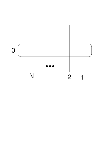
Figure 1: Closed-chain transfer matrix.

$$\tau_{closed}(\theta|\theta_{1}\,,\ldots\,,\theta_{N})=\mathop{\rm tr}\nolimits_{0}\{S_{0N}(\theta-\theta_{N})\cdots S_{02}(\theta-\theta_{2})\ S_{01}(\theta-\theta_{1})\}\,,$$ (3.3)

with inhomogeneities $\theta_{1}\,,\ldots\,,\theta_{N}$. Notice that we have introduced an additional (“auxiliary”) 2-dimensional vector space denoted by $0$. The product of $S$ matrices inside the trace (the so-called monodromy matrix) acts on $V^{\otimes(N+1)}$; but after performing the trace over the auxiliary space, one is left with an operator which acts on the (“quantum”) space $V^{\otimes N}$. Because $S(\theta)$ satisfies the Yang-Baxter equation, the transfer matrix commutes for different values of $\theta$

$$\left[\tau_{closed}(\theta|\theta_{1}\,,\ldots\,,\theta_{N})\,,\tau_{closed}(\theta^{\prime}|\theta_{1}\,,\ldots\,,\theta_{N})\right]=0\,.$$ (3.4)

Let us now evaluate this transfer matrix at $\theta=\theta_{1}$. Using the fact that $S(0)={\cal P}$ (the permutation matrix (2.22)) and ${\cal P}^{2}=\mathbb{I}$, we see that

$$\tau_{closed}(\theta_{1}|\theta_{1}\,,\ldots\,,\theta_{N})=\mathop{\rm tr}\nolimits_{0}\{({\cal P}_{01}{\cal P}_{01})S_{0N}(\theta_{1}-\theta_{N})\cdots({\cal P}_{01}{\cal P}_{01})S_{02}(\theta_{1}-\theta_{2})\ {\cal P}_{01}\}\,.$$ (3.5)

Finally, using ${\cal P}_{01}\ S_{0i}\ {\cal P}_{01}=S_{1i}$ and $\mathop{\rm tr}\nolimits_{0}{\cal P}_{01}=\mathbb{I}_{1}$, we conclude that $\tau_{closed}(\theta_{1}|\theta_{1}\,,\ldots\,,\theta_{N})=Y_{(1)}$. In general, we have

$$Y_{(i)}=\tau_{closed}(\theta_{i}|\theta_{1}\,,\ldots\,,\theta_{N})\,,\qquad i=1\,,\ldots\,,N\,.$$ (3.6)

This is the sought-after relation. In order to diagonalize the Yang matrices $Y_{(i)}$, it suffices to diagonalize the commuting closed-chain transfer matrix $\tau_{closed}(\theta|\theta_{1}\,,\ldots\,,\theta_{N})$. That calculation, as well as the corresponding bulk TBA analysis, is described in [6].

3.2 Open

We now turn to the case with boundaries, which is our primary interest in this paper. We therefore consider $N$ particles of mass $m$ with real rapidities $\theta_{1}\,,\ldots\,,\theta_{N}$ in an interval of length $L>>{1\over m}$, with bulk $S$ matrix $S(\theta)$ (2.28) and boundary $S$ matrix $\mathsf{S}(\theta\,;\xi)$ (2.60). The Yang equation for particle 1 is given by [30], [31]

$$\left(e^{2iLm\sinh\theta_{1}}Y_{(1)}-\mathbb{I}\right)|\theta_{1}\,,\ldots\theta_{N}\rangle=0\,,$$ (3.7)

where the Yang matrix $Y_{(1)}$ is now given by

$$Y_{(1)}=\mathsf{S}_{1}(\theta_{1}\,;\xi_{-})\ S_{21}(\theta_{1}+\theta_{2})\cdots S_{N1}(\theta_{1}+\theta_{N})\ \mathsf{S}_{1}(\theta_{1}\,;\xi_{+})\ S_{1N}(\theta_{1}-\theta_{N})\cdots S_{12}(\theta_{1}-\theta_{2})\,,$$ (3.8)

where the subscripts $\pm$ denote the left and right boundaries. (There are similar matrices $Y_{(i)}$ for the other particles.) In analogy with the case of periodic boundary conditions, the key to diagonalizing the Yang matrix is to relate it to an inhomogeneous open-chain transfer matrix [46] (see Figure 2)

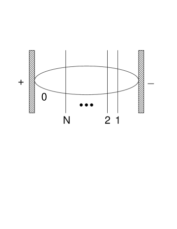
Figure 2: Open-chain transfer matrix.

$$\tau(\theta|\theta_{1}\,,\ldots\,,\theta_{N}) = \mathop{\rm tr}\nolimits_{0}\{\mathsf{S}_{0}(-\theta+i\pi\,;\xi_{+})^{t_{0}}\ S_{0N}(\theta-\theta_{N})\cdots S_{01}(\theta-\theta_{1})$$ (3.9)

$$\times \mathsf{S}_{0}(\theta\,;\xi_{-})\ S_{01}(\theta+\theta_{1})\cdots S_{0N}(\theta+\theta_{N})\}\,,$$

which commutes for different values of $\theta$

$$\left[\tau(\theta|\theta_{1}\,,\ldots\,,\theta_{N})\,,\tau(\theta^{\prime}|\theta_{1}\,,\ldots\,,\theta_{N})\right]=0\,.$$ (3.10)

Using the boundary cross-unitarity relation (2.46) as well as the Yang-Baxter equation (2.16), (2.45), one can show that

$$Y_{(i)}=\tau(\theta_{i}|\theta_{1}\,,\ldots\,,\theta_{N})\,,\qquad i=1\,,\ldots\,,N\,.$$ (3.11)

A proof for the case $N=2$ is presented in Appendix A. Hence, in order to diagonalize the Yang matrices $Y_{(i)}$, it suffices to diagonalize the commuting open-chain transfer matrix $\tau(\theta|\theta_{1}\,,\ldots\,,\theta_{N})$. It is to this task that we devote the following section.

4 Inversion identity and transfer-matrix eigenvalues

In this Section, we consider the problem of determining the eigenvalues of the inhomogeneous open-chain transfer matrix (3.9). Our approach will be to first derive an exact so-called inversion identity. This approach has been used in the past to diagonalize simple (e.g., Ising) closed-chain transfer matrices [47],[15],[6].

4.1 Inversion identity

Instead of working with the “dressed” transfer matrix (3.9), it is more convenient (see Footnote 9 below) to strip away the scalar factors from the bulk and boundary $S$ matrices, and to work instead with the “bare” transfer matrix

$$\mathfrak{t}(\theta|\theta_{1}\,,\ldots\,,\theta_{N}) = \mathop{\rm tr}\nolimits_{0}\{\mathsf{R}_{0}(-\theta+i\pi\,;\varphi_{+})^{t_{0}}\ R_{0N}(\theta-\theta_{N})\cdots R_{01}(\theta-\theta_{1})$$ (4.1)

$$\times \mathsf{R}_{0}(\theta\,;\varphi_{-})\ R_{01}(\theta+\theta_{1})\cdots R_{0N}(\theta+\theta_{N})\}\,,$$

where $R(\theta)$ is given by (2.13) and $\mathsf{R}(\theta\,;\varphi)$ is given by (2.40) with $\varepsilon=+1$.

There are two key points involved in obtaining the inversion identity. The first key point is to observe that the bulk $S$ matrix degenerates into a one-dimensional projector for a certain value of $\theta\ (=-i\pi)$:

$$S(-i\pi)\propto{1\over 2}\left(\begin{array}[]{rrrr}1&0&0&-1\\ 0&0&0&0\\ 0&0&0&0\\ -1&0&0&1\end{array}\right)\,.$$ (4.6)

Hence, it is possible to “fuse” [48],[49],[41] in the auxiliary space, and thereby obtain a fusion formula of the form [32]

$$\mathfrak{t}(\theta|\theta_{1}\,,\ldots\,,\theta_{N})\ \mathfrak{t}(\theta+i\pi|\theta_{1}\,,\ldots\,,\theta_{N})\propto\tilde{}\mathfrak{t}(\theta|\theta_{1}\,,\ldots\,,\theta_{N})+\Delta\,,$$ (4.7)

where $\tilde{}\mathfrak{t}(\theta|\theta_{1}\,,\ldots\,,\theta_{N})$ is a “fused” open-chain transfer matrix (see Figure 3), and here $\Delta$ represents a product of certain quantum determinants [50]. The fused transfer matrix is constructed from the fused bulk $S$ matrix $\tilde{R}(\theta)$ and the fused boundary $S$ matrix $\tilde{}\mathsf{R}(\theta\,;\varphi)$ , using the “fused” 3-dimensional (instead of 2-dimensional) auxiliary space.

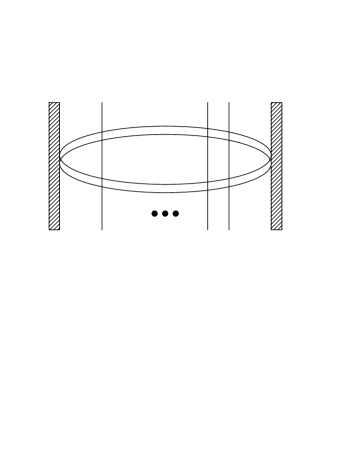
Figure 3: Fused open-chain transfer matrix.

The second key point is that both $\tilde{R}(\theta)$ and $\tilde{}\mathsf{R}(\theta\,;\varphi)$ can be brought to upper-triangular form by a $\theta$-independent similarity transformation. This remarkable fact is presumably due to the fact that $R(\theta)$ satisfies the free Fermion condition (2.15) (cf, [34]). As a result, the fused transfer matrix is proportional to the identity matrix

$$\tilde{}\mathfrak{t}(\theta|\theta_{1}\,,\ldots\,,\theta_{N})\propto\mathbb{I}\,.$$ (4.8)

It follows from the fusion formula that the transfer matrix obeys an exact inversion identity

$$\mathfrak{t}(\theta|\theta_{1}\,,\ldots\,,\theta_{N})\ \mathfrak{t}(\theta+i\pi|\theta_{1}\,,\ldots\,,\theta_{N})=f(\theta)\mathbb{I}\,,$$ (4.9)

where $f(\theta)$ is a calculable scalar function. We find (see Appendix B for more details)

$$f(\theta)={16\sinh^{2}\theta\over\sinh(\theta-iB\pi)\sinh(\theta+iB\pi)(1+\sin B\pi)^{2}\sin^{2}B\pi}\Big{\{}$$ (4.10)

$$\Big{(}\mathfrak{a}\prod_{j=1}^{N}{\cosh({1\over 2}(\theta-\theta_{j})-iB\pi)\over\cosh({1\over 2}(\theta-\theta_{j}))}{\cosh({1\over 2}(\theta+\theta_{j})-iB\pi)\over\cosh({1\over 2}(\theta+\theta_{j}))}$$

$$-\mathfrak{b}\prod_{j=1}^{N}{\sinh({1\over 2}(\theta-\theta_{j})-iB\pi)\over\sinh({1\over 2}(\theta-\theta_{j}))}{\sinh({1\over 2}(\theta+\theta_{j})-iB\pi)\over\sinh({1\over 2}(\theta+\theta_{j}))}\Big{)}$$

$$\times\Big{(}\mathfrak{c}\prod_{j=1}^{N}{\cosh({1\over 2}(\theta-\theta_{j})+iB\pi)\over\cosh({1\over 2}(\theta-\theta_{j}))}{\cosh({1\over 2}(\theta+\theta_{j})+iB\pi)\over\cosh({1\over 2}(\theta+\theta_{j}))}$$

$$-\mathfrak{d}\prod_{j=1}^{N}{\sinh({1\over 2}(\theta-\theta_{j})+iB\pi)\over\sinh({1\over 2}(\theta-\theta_{j}))}{\sinh({1\over 2}(\theta+\theta_{j})+iB\pi)\over\sinh({1\over 2}(\theta+\theta_{j}))}\Big{)}\Big{\}}\,,$$

where

$$\mathfrak{a} = \sinh^{2}({1\over 2}(i\pi B+{i\pi\over 2}-\theta))\left[e^{-\varphi_{-}}\sinh^{2}({1\over 2}(i\pi B+{i\pi\over 2}))+e^{\varphi_{-}}\sinh^{2}({1\over 2}(-i\pi B+{i\pi\over 2}+\theta))\right]\times\left[\varphi_{-}\rightarrow\varphi_{+}\right]$$

$$\mathfrak{b} = \sinh^{2}({1\over 2}(-i\pi B+{i\pi\over 2}+\theta))\left[e^{-\varphi_{-}}\sinh^{2}({1\over 2}(i\pi B+{i\pi\over 2}))+e^{\varphi_{-}}\sinh^{2}({1\over 2}(i\pi B+{i\pi\over 2}-\theta))\right]\times\left[\varphi_{-}\rightarrow\varphi_{+}\right]$$

$$\mathfrak{c} = \sinh^{2}({1\over 2}(i\pi B+{i\pi\over 2}+\theta))\left[e^{-\varphi_{-}}\sinh^{2}({1\over 2}(i\pi B+{i\pi\over 2}))+e^{\varphi_{-}}\sinh^{2}({1\over 2}(i\pi B-{i\pi\over 2}+\theta))\right]\times\left[\varphi_{-}\rightarrow\varphi_{+}\right]$$

$$\mathfrak{d} = \sinh^{2}({1\over 2}(i\pi B-{i\pi\over 2}+\theta))\left[e^{-\varphi_{-}}\sinh^{2}({1\over 2}(i\pi B+{i\pi\over 2})+e^{\varphi_{-}}\sinh^{2}({1\over 2}(i\pi B+{i\pi\over 2}+\theta))\right]\times\left[\varphi_{-}\rightarrow\varphi_{+}\right]\,.$$

Notice that the function $f(\theta)$ is invariant under the duality transformation $B\rightarrow 1-B$. This inversion identity is one of the main results of this paper. We have checked it numerically up to $N=3$.

4.2 Eigenvalues

We now proceed to determine the eigenvalues of the transfer matrix. First, observe that by virtue of the commutativity property (3.10), the bare transfer matrix $\mathfrak{t}(\theta|\theta_{1}\,,\ldots\,,\theta_{N})$ has eigenstates $|\theta_{1}\,,\ldots\theta_{N}\rangle$ which are independent of $\theta$,

$$\mathfrak{t}(\theta|\theta_{1}\,,\ldots\,,\theta_{N})|\theta_{1}\,,\ldots\theta_{N}\rangle=\mathfrak{L}(\theta|\theta_{1}\,,\ldots\,,\theta_{N})|\theta_{1}\,,\ldots\theta_{N}\rangle\,,$$ (4.12)

where $\mathfrak{L}(\theta|\theta_{1}\,,\ldots\,,\theta_{N})$ are the corresponding eigenvalues. Acting on $|\theta_{1}\,,\ldots\theta_{N}\rangle$ with the inversion identity, we obtain the corresponding identity for the eigenvalues

$$\mathfrak{L}(\theta|\theta_{1}\,,\ldots\,,\theta_{N})\ \mathfrak{L}(\theta+i\pi|\theta_{1}\,,\ldots\,,\theta_{N})=f(\theta)\,.$$ (4.13)

Moreover, one can show that the bare transfer matrix $\mathfrak{t}(\theta|\theta_{1}\,,\ldots\,,\theta_{N})$ is a periodic function of $\theta$ with period $2\pi i$

$$\mathfrak{t}(\theta+2\pi i|\theta_{1}\,,\ldots\,,\theta_{N})=\mathfrak{t}(\theta|\theta_{1}\,,\ldots\,,\theta_{N})\,,$$ (4.14)

whose asymptotic behavior for large $\theta$ is given by

$$\mathfrak{t}(\theta|\theta_{1}\,,\ldots\,,\theta_{N})\sim{c\over 32}e^{3\theta}\mathbb{I}\quad\mbox{ for }\quad\theta\rightarrow\infty\,,$$ (4.15)

where

$$c={4ie^{\varphi_{-}+\varphi_{+}}\over(1+\sin B\pi)\sin B\pi}\,.$$ (4.16)

Correspondingly, the eigenvalues obey

$$\mathfrak{L}(\theta+2\pi i|\theta_{1}\,,\ldots\,,\theta_{N}) = \mathfrak{L}(\theta|\theta_{1}\,,\ldots\,,\theta_{N})\,,$$

$$\mathfrak{L}(\theta|\theta_{1}\,,\ldots\,,\theta_{N}) \sim {c\over 32}e^{3\theta}\quad\mbox{ for }\quad\theta\rightarrow\infty\,.$$ (4.17)

The eigenvalues $\mathfrak{L}(\theta|\theta_{1}\,,\ldots\,,\theta_{N})$ are uniquely determined by the zeros and poles of $f(\theta)$, together with periodicity and asymptotic behavior. Indeed, observe that $f(\theta)$ is a product of two factors. Let $\theta=z_{k}^{+}\,,z_{k}^{-}$ be zeros of the first, second factors, respectively. Then $z_{k}^{+}$ obeys

$$\prod_{j=1}^{N}{\tanh({1\over 2}(z_{k}^{+}-\theta_{j})-iB\pi)\over\tanh({1\over 2}(z_{k}^{+}-\theta_{j}))}{\tanh({1\over 2}(z_{k}^{+}+\theta_{j})-iB\pi)\over\tanh({1\over 2}(z_{k}^{+}+\theta_{j}))}={\sinh^{2}({1\over 2}(i\pi B+{i\pi\over 2}-z_{k}^{+}))\over\sinh^{2}({1\over 2}(-i\pi B+{i\pi\over 2}+z_{k}^{+}))}$$ (4.18)

$$\times \left[{e^{-\varphi_{-}}\sinh^{2}({1\over 2}(i\pi B+{i\pi\over 2}))+e^{\varphi_{-}}\sinh^{2}({1\over 2}(-i\pi B+{i\pi\over 2}+z_{k}^{+}))\over e^{-\varphi_{-}}\sinh^{2}({1\over 2}(i\pi B+{i\pi\over 2}))+e^{\varphi_{-}}\sinh^{2}({1\over 2}(i\pi B+{i\pi\over 2}-z_{k}^{+}))}\right]\times\left[\varphi_{-}\rightarrow\varphi_{+}\right]\,,$$

and $z_{k}^{-}$ obeys

$$\prod_{j=1}^{N}{\tanh({1\over 2}(z_{k}^{-}-\theta_{j})+iB\pi)\over\tanh({1\over 2}(z_{k}^{-}-\theta_{j}))}{\tanh({1\over 2}(z_{k}^{-}+\theta_{j})+iB\pi)\over\tanh({1\over 2}(z_{k}^{-}+\theta_{j}))}={\sinh^{2}({1\over 2}(i\pi B+{i\pi\over 2}+z_{k}^{-}))\over\sinh^{2}({1\over 2}(i\pi B-{i\pi\over 2}+z_{k}^{-}))}$$ (4.19)

$$\times \left[{e^{-\varphi_{-}}\sinh^{2}({1\over 2}(i\pi B+{i\pi\over 2}))+e^{\varphi_{-}}\sinh^{2}({1\over 2}(i\pi B-{i\pi\over 2}+z_{k}^{-}))\over e^{-\varphi_{-}}\sinh^{2}({1\over 2}(i\pi B+{i\pi\over 2}))+e^{\varphi_{-}}\sinh^{2}({1\over 2}(i\pi B+{i\pi\over 2}+z_{k}^{-}))}\right]\times\left[\varphi_{-}\rightarrow\varphi_{+}\right]\,.$$

These are our “magnonic” Bethe Ansatz equations.

It follows that $f(\theta)$ can be represented as

$$f(\theta)=-{c^{2}\over 16}\sinh^{2}\theta{\prod_{k=0}^{N}\sinh(\theta-z_{k}^{+})\sinh(\theta+z_{k}^{+})\sinh(\theta-z_{k}^{-})\sinh(\theta+z_{k}^{-})\over\prod_{k=1}^{N}\sinh^{2}(\theta-\theta_{k})\sinh^{2}(\theta+\theta_{k})}\,.$$ (4.20)

It now follows by similar arguments that

$$\mathfrak{L}(\theta|\theta_{1}\,,\ldots\,,\theta_{N})=c\sinh\theta{\prod_{k=0}^{N}\sinh({1\over 2}(\theta-z_{k}^{+}))\sinh({1\over 2}(\theta+z_{k}^{+}))\sinh({1\over 2}(\theta-z_{k}^{-}))\sinh({1\over 2}(\theta+z_{k}^{-}))\over\prod_{k=1}^{N}\sinh({1\over 2}(\theta-\theta_{k}))\sinh({1\over 2}(\theta+\theta_{k}))\cosh({1\over 2}(\theta-\theta_{k}))\cosh({1\over 2}(\theta+\theta_{k}))}\,.$$

(4.21)

is the unique solution to the inversion identity (4.13) with the properties (4.17). Note that there are $N+1$ pairs of roots $z_{k}^{\pm}$, whereas in the case of periodic boundary conditions [6] there are only $N$. The appearance of the additional pair of roots $z_{0}^{\pm}$ is due to the fact that the boundary $S$ matrix $\mathsf{R}(\theta\,;\varphi)$ is not diagonal. The existence of these roots is essential for obtaining the correct asymptotic behavior; and it can be easily checked for the case $N=0$.

In summary, the eigenvalues of the bare transfer matrix (4.1) are given by (4.21), where $z_{k}^{\pm}$ satisfy Eqs. (4.18), (4.19).

4.3 Structure of Bethe Ansatz roots

Before performing the thermodynamic ($N\rightarrow\infty$) limit (which is the subject of the next section), it is necessary to first understand the structure of the Bethe Ansatz roots. Following [6], we observe that the Bethe Ansatz Eqs. (4.18), (4.19) have roots of the form

$$z_{k}^{+}=\left\{\begin{array}[]{c}x_{k}+iB\pi\\ x_{k}+iB\pi+i\pi\end{array}\right.\,,\qquad z_{k}^{-}=\left\{\begin{array}[]{c}x_{k}-iB\pi\\ x_{k}-iB\pi-i\pi\end{array}\right.\,,$$ (4.26)

where $x_{k}$ are real and satisfy

$$\prod_{j=1}^{N}\left[{\tanh({1\over 2}(x_{k}-\theta_{j}-iB\pi))\over\tanh({1\over 2}(x_{k}-\theta_{j}+iB\pi))}{\tanh({1\over 2}(x_{k}+\theta_{j}-iB\pi))\over\tanh({1\over 2}(x_{k}+\theta_{j}+iB\pi))}\right]{\sinh^{2}({1\over 2}({i\pi\over 2}+x_{k}))\over\sinh^{2}({1\over 2}({i\pi\over 2}-x_{k}))}$$ (4.27)

$$\times \left[{e^{-\varphi_{-}}\sinh^{2}({1\over 2}(i\pi B+{i\pi\over 2}))+e^{\varphi_{-}}\sinh^{2}({1\over 2}({i\pi\over 2}-x_{k}))\over e^{-\varphi_{-}}\sinh^{2}({1\over 2}(i\pi B+{i\pi\over 2}))+e^{\varphi_{-}}\sinh^{2}({1\over 2}({i\pi\over 2}+x_{k}))}\right]\times\left[\varphi_{-}\rightarrow\varphi_{+}\right]=1\,,$$

$$\qquad k=0\,,1\,,\ldots\,,N\,.$$

Evidently, for each $x_{k}$, there are 4 possible combinations of roots $(z_{k}^{+}\,,z_{k}^{-})$. However, by considering the limit $B\rightarrow 0$, one can argue that only 2 of these combinations are allowed, which we denote by $\epsilon_{k}=+1$ and $\epsilon_{k}=-1$, respectively:

$$\epsilon_{k} = +1:\qquad(z_{k}^{+}=x_{k}+iB\pi\,,\quad z_{k}^{-}=x_{k}-iB\pi-i\pi)\,,$$

$$\epsilon_{k} = -1:\qquad(z_{k}^{+}=x_{k}+iB\pi+i\pi\,,\quad z_{k}^{-}=x_{k}-iB\pi)\,.$$ (4.28)

Hence, the eigenvalues are specified by $\{x_{k}\,,\epsilon_{k}\}$, $k=0\,,\ldots\,,N$:

$$\mathfrak{L}(\theta|\theta_{1}\,,\ldots\,,\theta_{N})_{\epsilon_{0}\cdots\epsilon_{N}}=c\sinh\theta{\prod_{k=0}^{N}\lambda_{\epsilon_{k}}(\theta-x_{k})\ \lambda_{-\epsilon_{k}}(\theta+x_{k})\over\prod_{k=1}^{N}{1\over 4}\sinh(\theta-\theta_{k})\sinh(\theta+\theta_{k})}\,,$$ (4.29)

where

$$\lambda_{\epsilon}(\theta)=\sinh({1\over 2}(\theta-\epsilon iB\pi))\cosh({1\over 2}(\theta+\epsilon iB\pi))\,,$$ (4.30)

$\epsilon_{k}=\pm 1$, and $x_{k}$ satisfy (4.27).

To close this section, we observe that the “dressed” transfer matrix (3.9) is simply related to the “bare” transfer matrix (4.1) by

$$\tau(\theta|\theta_{1}\,,\ldots\,,\theta_{N})=\mathsf{Z}(-\theta+i\pi\,;\xi_{+})\mathsf{Z}(\theta\,;\xi_{-})\prod_{k=1}^{N}\left[Z(\theta-\theta_{k})Z(\theta+\theta_{k})\right]\mathfrak{t}(\theta|\theta_{1}\,,\ldots\,,\theta_{N})\,,$$ (4.31)

where the scalar factors $Z(\theta)$ and $\mathsf{Z}(\theta\,;\xi)$ are introduced in Eqs. (2.25), (2.59). Hence, the eigenvalues $\Lambda(\theta|\theta_{1}\,,\ldots\,,\theta_{N})$ of $\tau(\theta|\theta_{1}\,,\ldots\,,\theta_{N})$ are given by

$$\Lambda(\theta|\theta_{1}\,,\ldots\,,\theta_{N})_{\epsilon_{0}\cdots\epsilon_{N}} = {\mathsf{Z}(\theta\,;\xi_{+})\ \mathsf{Z}(\theta\,;\xi_{-})\ Z(-2\theta)\over g({i\pi\over 2}-\theta)}\prod_{k=1}^{N}Z(\theta-\theta_{k})Z(\theta+\theta_{k})$$ (4.32)

$$\times \mathfrak{L}(\theta|\theta_{1}\,,\ldots\,,\theta_{N})_{\epsilon_{0}\cdots\epsilon_{N}}\,,$$

where $\mathfrak{L}(\theta|\theta_{1}\,,\ldots\,,\theta_{N})_{\epsilon_{0}\cdots\epsilon_{N}}$ is given by (4.29). Here we have used the fact

$$\mathsf{Z}(-\theta+i\pi\,;\xi)={\mathsf{Z}(\theta\,;\xi)Z(-2\theta)\over g({i\pi\over 2}-\theta)}\,,$$ (4.33)

which follows from the bulk unitarity (2.7), (2.24) and boundary cross-unitarity (2.36), (2.55), (2.56) relations.

5 Thermodynamic Bethe Ansatz analysis

Having obtained the eigenvalues of the transfer matrix and the Bethe Ansatz equations, we can proceed to the derivation of the TBA equations and boundary entropy. We begin by briefly reviewing the general framework. Following [8],[17] we consider the partition function $Z_{+-}$ of the system on a cylinder of length $L$ and circumference $R$ with left/right boundary conditions denoted by $\pm$ (see Figure 4)

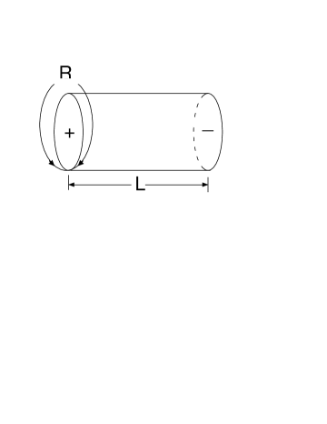
Figure 4: Cylinder on which the partition function $Z_{+-}$ is defined.

$$Z_{+-} = \mathop{\rm tr}\nolimits e^{-RH_{+-}}=e^{-RF}$$ (5.1)

$$= \langle B_{+}|e^{-LH_{P}}|B_{-}\rangle$$

$$\approx \langle B_{+}|0\rangle\langle 0|B_{-}\rangle e^{-LE_{0}}\qquad\mbox{ for }L\rightarrow\infty\,.$$

In the first line, Euclidean time evolves along the circumference of the cylinder, and $H_{+-}$ is the Hamiltonian for the system with spatial boundary conditions $\pm$. In passing to the second line, we rotate the picture, so that time evolves parallel to the axis of the cylinder; $H_{P}$ is the Hamiltonian for the system with periodic boundary conditions, and $|B_{\pm}\rangle$ are boundary states which encode initial/final (temporal) conditions. In the third line, we consider the limit $L\rightarrow\infty$; the state $|0\rangle$ is the ground state of $H_{P}$, and $E_{0}$ is the corresponding eigenvalue. The quantity $\ln\langle B_{+}|0\rangle\langle 0|B_{-}\rangle$ is the sought-after boundary entropy [20],[17]. Taking the logarithm of the above expressions for the partition function, one obtains

$$-RF\approx-LE_{0}+\ln\langle B_{+}|0\rangle\langle 0|B_{-}\rangle\,.$$ (5.2)

Whereas the free energy $F$ has a leading contribution which is of order $L$, here we seek the subleading correction which is of order $1$.

5.1 Thermodynamic limit

We proceed to compute $F$ using the TBA approach [6], [13]-[17]. To this end, we introduce the densities $P_{\pm}(\theta)$ of “magnons”, i.e., of real Bethe Ansatz roots $\{x_{k}\}$ with $\epsilon_{k}=\pm 1$, respectively; and also the densities $\rho_{1}(\theta)$ and $\tilde{\rho}(\theta)$ of particles $\{\theta_{k}\}$ and holes, respectively. Computing the logarithmic derivative of the “magnonic” Bethe Ansatz equations (4.27), we obtain

$$P_{+}(\theta)+P_{-}(\theta) = {1\over 2\pi}\int_{0}^{\infty}d\theta^{\prime}\ \rho_{1}(\theta^{\prime})\left[\Phi(\theta-\theta^{\prime})+\Phi(\theta+\theta^{\prime})\right]$$ (5.3)

$$+ {1\over 2\pi L}\left[-\Phi(\theta)+2\Psi(\theta)+\Psi_{\varphi_{+}}(\theta)+\Psi_{\varphi_{-}}(\theta)\right]\,,$$

where

$$\Phi(\theta) = {1\over i}{\partial\over\partial\theta}\ln\left({\tanh({1\over 2}(\theta-iB\pi))\over\tanh({1\over 2}(\theta+iB\pi))}\right)={4\cosh\theta\sin B\pi\over\cosh 2\theta-\cos 2B\pi}\,,$$

$$\Psi(\theta) = {1\over i}{\partial\over\partial\theta}\ln\left({\sinh({1\over 2}({i\pi\over 2}+\theta))\over\sinh({1\over 2}({i\pi\over 2}-\theta))}\right)=-{1\over\cosh\theta}\,,$$

$$\Psi_{\varphi}(\theta) = {1\over i}{\partial\over\partial\theta}\ln\left({e^{-\varphi}\sinh^{2}({1\over 2}(i\pi B+{i\pi\over 2}))+e^{\varphi}\sinh^{2}({1\over 2}({i\pi\over 2}-\theta))\over e^{-\varphi}\sinh^{2}({1\over 2}(i\pi B+{i\pi\over 2}))+e^{\varphi}\sinh^{2}({1\over 2}({i\pi\over 2}+\theta))}\right)$$ (5.4)

$$= {4\cosh\theta\cos\zeta\over\cosh 2\theta+\cos 2\zeta}\,,$$

where $\zeta$ is defined in (2.58). Defining $\rho_{1}(\theta)$ for negative values of $\theta$ to be equal to $\rho_{1}(|\theta|)$, we obtain the final form

$$P_{+}(\theta)+P_{-}(\theta)={1\over 2\pi}\left(\rho_{1}*\Phi\right)(\theta)+{1\over 2\pi L}\left[-\Phi(\theta)+2\Psi(\theta)+\Psi_{\varphi_{+}}(\theta)+\Psi_{\varphi_{-}}(\theta)\right]\,,$$ (5.5)

where $*$ denotes convolution

$$\left(f*g\right)(\theta)=\int_{-\infty}^{\infty}d\theta^{\prime}\ f(\theta-\theta^{\prime})g(\theta^{\prime})\,.$$ (5.6)

We next consider the Yang equations, which imply (see Eqs. (3.7),(3.11))

$$e^{2iLm\sinh\theta_{k}}\Lambda(\theta_{k}|\theta_{1}\,,\ldots\,,\theta_{N})=1\,,\qquad k=1\,,\ldots\,,N\,,$$ (5.7)

where $\Lambda(\theta|\theta_{1}\,,\ldots\,,\theta_{N})$ is the eigenvalue of the dressed transfer matrix $\tau(\theta|\theta_{1}\,,\ldots\,,\theta_{N})$, which is given by (4.32). Computing the logarithmic derivative, we obtain

$$\rho_{1}(\theta)+\tilde{\rho}(\theta) = {1\over 2\pi}\Big{\{}2m\cosh\theta+\int_{0}^{\infty}d\theta^{\prime}\ \rho_{1}(\theta^{\prime})\left[\Phi_{Z}(\theta-\theta^{\prime})+\Phi_{Z}(\theta+\theta^{\prime})\right]$$ (5.8)

$$+ \int_{0}^{\infty}d\theta^{\prime}\ \Big{[}P_{+}(\theta^{\prime})\Phi_{+}(\theta-\theta^{\prime})+P_{-}(\theta^{\prime})\Phi_{-}(\theta-\theta^{\prime})$$

$$+ P_{-}(\theta^{\prime})\Phi_{+}(\theta+\theta^{\prime})+P_{+}(\theta^{\prime})\Phi_{-}(\theta+\theta^{\prime})\Big{]}$$

$$+ {1\over L}\left[-\Phi_{Z}(\theta)-2\Phi_{Z}(2\theta)+{\partial\over\partial\theta}Im\ln\mathsf{Z}(\theta\,;\xi_{+})+{\partial\over\partial\theta}Im\ln\mathsf{Z}(\theta\,;\xi_{-})\right]\Big{\}}\,,$$

where

$$\Phi_{Z}(\theta)={\partial\over\partial\theta}Im\ln Z(\theta)\,,\qquad\Phi_{\pm}(\theta)={\partial\over\partial\theta}Im\ln\lambda_{\pm}(\theta)\,.$$ (5.9)

Using the fact $\Phi_{\pm}(\theta)=\pm{1\over 2}\Phi(\theta)$, and defining $P_{\pm}(\theta)$ for negative values of $\theta$ to be equal to $-P_{\pm}(|\theta|)$, we obtain

$$\rho_{1}(\theta)+\tilde{\rho}(\theta) = {m\over\pi}\cosh\theta+{1\over 2\pi}\left(\rho_{1}*\Phi_{Z}\right)(\theta)+{1\over 4\pi}\left((P_{+}-P_{-})*\Phi\right)(\theta)$$ (5.10)

$$+ {1\over 2\pi L}\left[-\Phi_{Z}(\theta)-2\Phi_{Z}(2\theta)+{\partial\over\partial\theta}Im\ln\mathsf{Z}(\theta\,;\xi_{+})+{\partial\over\partial\theta}Im\ln\mathsf{Z}(\theta\,;\xi_{-})\right]\,.$$

We now use (5.5) to eliminate $P_{-}$, and use the expressions (2.59), (2.63) to separate the various factors in $\mathsf{Z}(\theta\,;\xi)$ to obtain

$$\rho_{1}(\theta)+\tilde{\rho}(\theta) = {m\over\pi}\cosh\theta+{1\over 2\pi}P_{+}*\Phi+{1\over 2\pi}\rho_{1}*\left(\Phi_{Z}-{1\over 4\pi}\Phi*\Phi\right)$$

$$+ {1\over 2\pi L}\Bigg{[}-\left(\Phi_{Z}-{1\over 4\pi}\Phi*\Phi\right)+2\left({\partial\over\partial\theta}Im\ln\mathsf{Z}_{0}(\theta)-\Phi_{Z}(2\theta)-{1\over 4\pi}\Psi*\Phi\right)$$

$$+ \left({\partial\over\partial\theta}Im\ln\mathsf{Y}_{1}(\theta\,;\varphi_{+})-{1\over 4\pi}\Psi_{\varphi_{+}}*\Phi\right)+\left({\partial\over\partial\theta}Im\ln\mathsf{Y}_{1}(\theta\,;\varphi_{-})-{1\over 4\pi}\Psi_{\varphi_{-}}*\Phi\right)$$

$$+ {1\over i}{\partial\over\partial\theta}\ln\mathsf{X}_{1}(\theta\,;{4\eta_{+}B\over\pi})\ \mathsf{X}_{1}(\theta\,;{4i\vartheta_{+}B\over\pi})+{1\over i}{\partial\over\partial\theta}\ln\mathsf{X}_{1}(\theta\,;{4\eta_{-}B\over\pi})\ \mathsf{X}_{1}(\theta\,;{4i\vartheta_{-}B\over\pi})\Bigg{]}\,.$$

Noting the “bulk” identity [27]

$$\Phi_{Z}(\theta)-{1\over 4\pi}\left(\Phi*\Phi\right)(\theta)=0\,,$$ (5.12)

and its boundary counterparts

$${\partial\over\partial\theta}Im\ln\mathsf{Y}_{1}(\theta\,;\varphi)-{1\over 4\pi}\left(\Psi_{\varphi}*\Phi\right)(\theta) = 0\,,$$

$${\partial\over\partial\theta}Im\ln\mathsf{Z}_{0}(\theta)-\Phi_{Z}(2\theta)-{1\over 4\pi}\left(\Psi*\Phi\right)(\theta) = -{1\over 4}\Phi(\theta)+\Psi(\theta)\,,$$ (5.13)

we remain with the rather simple result

$$\rho_{1}(\theta)+\tilde{\rho}(\theta) = {m\over\pi}\cosh\theta+{1\over 2\pi}\left(P_{+}*\Phi\right)(\theta)+{1\over 2\pi L}\Bigg{[}-{1\over 2}\Phi(\theta)+2\Psi(\theta)$$ (5.14)

$$+ \kappa(\theta\,;{4\eta_{+}B\over\pi})+\kappa(\theta\,;{4i\vartheta_{+}B\over\pi})+\kappa(\theta\,;{4\eta_{-}B\over\pi})+\kappa(\theta\,;{4i\vartheta_{-}B\over\pi})\Bigg{]}\,,$$

where

$$\kappa(\theta\,;F)={1\over i}{\partial\over\partial\theta}\ln\mathsf{X}_{1}(\theta\,;F)={4\cosh\theta\cos(\pi F/2)\over\cosh 2\theta+\cos\pi F}\,.$$ (5.15)

The thermodynamic limit of the magnonic Bethe Ansatz equations and the Yang equations, given by (5.5) and (5.14), respectively, are the main results of this subsection. Notice that the former depends on the boundary parameters $\varphi_{\pm}$, while the latter depends on the (boundary sinh-Gordon) boundary parameters $\eta_{\pm}\,,\vartheta_{\pm}$.

5.2 TBA equations and boundary entropy

The free energy $F$ is given by

$$F=E-TS\,,$$ (5.16)

where the temperature is $T={1\over R}$, the energy $E$ is

$$E=\sum_{k=1}^{N}m\cosh\theta_{k}={L\over 2}\int_{-\infty}^{\infty}d\theta\ \rho_{1}(\theta)m\cosh\theta\,,$$ (5.17)

and the entropy $S$ is [13],[15]

$$S = {L\over 2}\int_{-\infty}^{\infty}d\theta\ \Big{\{}(\rho_{1}+\tilde{\rho})\ln(\rho_{1}+\tilde{\rho})-\rho_{1}\ln\rho_{1}-\tilde{\rho}\ln\tilde{\rho}$$ (5.18)

$$+ (P_{+}+P_{-})\ln(P_{+}+P_{-})-P_{+}\ln P_{+}-P_{-}\ln P_{-}\Big{\}}\,.$$

Extremizing the free energy $(\delta F=0)$ subject to the constraints

$$\delta P_{-} = -\delta P_{+}+{1\over 2\pi}\delta\rho_{1}*\Phi\,,$$

$$\delta\tilde{\rho} = -\delta\rho_{1}+{1\over 2\pi}\delta P_{+}*\Phi\,,$$ (5.19)

(which follow from Eqs. (5.5), (5.14), respectively) we obtain a set of TBA equations which is the same as for the case of periodic boundary conditions [6],[27]

$$r\cosh\theta = \epsilon_{1}(\theta)+{1\over 2\pi}\left(\Phi*L_{2}\right)(\theta)\,,$$

$$0 = \epsilon_{2}(\theta)+{1\over 2\pi}\left(\Phi*L_{1}\right)(\theta)\,,$$ (5.20)

where

$$L_{i}(\theta) = \ln\left(1+e^{-\epsilon_{i}(\theta)}\right)\,,\qquad r=mR\,,$$

$$\epsilon_{1} = \ln\left({\tilde{\rho}\over\rho_{1}}\right)\,,\qquad\epsilon_{2}=\ln\left({P_{-}\over P_{+}}\right)\,.$$ (5.21)

We next evaluate $F$ using also the constraints (5.5), (5.14) and the TBA equations. From the boundary (order $1$) contribution, we obtain (see Eq. (5.2)) the boundary entropy

$$\ln\langle B_{+}|0\rangle\langle 0|B_{-}\rangle={1\over 4\pi}\int_{-\infty}^{\infty}d\theta\ \Big{\{} \Big{[}-{1\over 2}\Phi(\theta)+2\Psi(\theta)+\kappa(\theta\,;{4\eta_{+}B\over\pi})+\kappa(\theta\,;{4i\vartheta_{+}B\over\pi})$$ (5.22)

$$+ \kappa(\theta\,;{4\eta_{-}B\over\pi})+\kappa(\theta\,;{4i\vartheta_{-}B\over\pi})\Big{]}L_{1}(\theta)$$

$$+ \left[-\Phi(\theta)+2\Psi(\theta)+\Psi_{\varphi_{+}}(\theta)+\Psi_{\varphi_{-}}(\theta)\right]L_{2}(\theta)\,.$$

In particular, the dependence of the boundary entropy of a single boundary on the boundary parameters is given by

$$s_{B}(\eta\,,\vartheta\,,\varphi)={1\over 4\pi}\int_{-\infty}^{\infty}d\theta\ \left\{\left[\kappa(\theta\,;{4\eta B\over\pi})+\kappa(\theta\,;{4i\vartheta B\over\pi})\right]L_{1}(\theta)+\Psi_{\varphi}(\theta)\ L_{2}(\theta)\right\}\,,$$ (5.23)

where the kernels $\kappa(\theta\,;F)$ and $\Psi_{\varphi}(\theta)$ are defined in Eqs. (5.15) and (5.4), respectively. The term involving $L_{1}$, which had previously been conjectured [27], depends on the boundary sinh-Gordon parameters $\eta\,,\vartheta$. The term involving $L_{2}$, which had not been anticipated, depends on the boundary parameter $\varphi$ (which appears in $\mathsf{R}(\theta\,;\varphi)$, i.e., the non-diagonal part of the boundary $S$ matrix). This expression for the boundary entropy is another of the main results of this paper.

6 Boundary roaming trajectories

One application of our result (5.23) for the boundary entropy is to obtain boundary roaming trajectories corresponding to $c<3/2$ superconformal models. In order to best explain this result, it is helpful to first recall earlier work on bulk and boundary roaming.

Al. Zamolodchikov [23] first considered the TBA equations for the bulk ShG (non-supersymmetric) model with the coupling constant $\gamma$ analytically continued to complex values,

$$\gamma={\pi\over 2}\pm i\theta_{0}\,,\qquad\theta_{0}>>1\,.$$ (6.1)

The corresponding effective central charge $c_{eff}(r)$ interpolates (“roams”) between the values

$$c_{p}=1-{6\over p(p+1)}\,,\qquad p=3\,,4\,,5\,,\ldots$$ (6.2)

corresponding to the unitary $c<1$ minimal models [18]. Indeed, a plot of $c_{eff}(r)$ vs. $\log(r/2)$ reveals a “staircase” with plateaus at values of $c_{eff}(r)$ equal to $c_{p}$.

This result was later generalized [26] to the boundary ShG model: choosing the value of $r$ so that $c_{eff}(r)$ lies on some plateau, the boundary entropy $s_{B}(F)$ (where $F$ is a boundary parameter) interpolates between values corresponding to various conformal boundary conditions [19].

The original work [23] was also generalized [27] to the bulk SShG (supersymmetric) model. The TBA equations with a similar analytic continuation of the coupling constant

$$\pi B={\pi\over 2}\pm i\theta_{0}\,,\qquad\theta_{0}>>1$$ (6.3)

cause the effective central charge $c_{eff}(r)$ to interpolate between the values

$$c_{p}={3\over 2}\left(1-{8\over p(p+2)}\right)\,,\qquad p=4\,,6\,,8\,,\ldots$$ (6.4)

corresponding to the even unitary $c<3/2$ minimal models [21], [22]. Precisely this set of TBA equations had been conjectured earlier in [24], and then further generalized in [25].

Finally, let us consider the model of primary interest here, namely, boundary SShG. For simplicity, we fix $\phi_{0}=0$ in the boundary Lagrangian (2.30), which corresponds to $\vartheta=0$. Due to the roaming limit (6.3), we should rescale the remaining two parameters $\eta,\varphi$ so that the boundary entropy can be a function of well-defined (finite) boundary parameters. For this purpose we set $\eta\to 0$ and $\varphi\to\infty$ while keeping $\theta_{0}\eta$ and $\theta_{0}-2\varphi$ finite. Let us introduce new boundary parameters $f_{1}$ and $f_{2}$ defined by (see Eq. (2.58))

$${2\theta_{0}\eta\over{\pi}}\equiv f_{1},\qquad 1+{1\over{2}}e^{\theta_{0}-2\varphi}\equiv\cosh f_{2}\,.$$ (6.5)

We can reexpress the boundary entropy (5.23) in terms of these parameters as

$$s_{B}=s_{B}^{(1)}+s_{B}^{(2)}\,,\qquad\mbox{ where }\qquad s_{B}^{(i)}={1\over{4\pi}}\int_{-\infty}^{\infty}d\theta\ \Psi(\theta;f_{i})\ L_{i}(\theta),\qquad i=1,2,$$ (6.6)

with

$$\Psi(\theta;f)={4\cosh\theta\cosh f\over{\cosh 2\theta+\cosh 2f}}.$$ (6.7)

To compute the roaming boundary entropy, we fix a value of $r$ where $c_{eff}(r)$ lies on a plateau (6.4). Then, as we change the boundary roaming parameters $f_{1}$ and $f_{2}$, we check if the boundary entropy interpolates between the values [27]

$$s_{B}(r\,,s) = \ln\left[\left({\sin({\pi r\over p})\over\sin({\pi\over p})}\right)\left({\sin({\pi s\over p+2})\over\sin({\pi\over p+2})}\right)\right]$$ (6.8)

$$= s_{B}(r\,,1)+s_{B}(1\,,s)\,.$$

corresponding to conformal boundary states $(r\,,s)$ (which, in turn, correspond to primary fields $\Phi_{(r\,,s)}$).

Indeed, we can see clearly from Figure 5 [27] that $s_{B}^{(1)}$ interpolates between boundary entropies of the conformal boundary states

Figure 5: Boundary roaming trajectories: $s_{B}^{(1)}$ vs. $f_{1}$.

$$(1\,,a)\leftrightarrow\left\{\begin{array}[]{c}(a-2\,,1)\\ (a\,,1)\end{array}\right.\,,\qquad a\mbox{ odd }\,.$$ (6.11)

Similarly $s_{B}^{(2)}$ generates the new flow (see Figure 6)

Figure 6: Boundary roaming trajectories: $s_{B}^{(2)}$ vs. $f_{2}$.

$$(1\,,a)\leftrightarrow\left\{\begin{array}[]{c}(a-2\,,1)\\ (a\,,1)\end{array}\right.\,,\qquad a\mbox{ even }\,.$$ (6.14)

While these flows are generated by changing one parameter while fixing the other, we can generate more general flows by changing $f_{1}$ and $f_{2}$ simultaneously. In view of the additivity property (6.8), these two sets of flows can be combined to generate additional flows for the total boundary entropy $s_{B}$

$$(r\,,s)\leftrightarrow\left\{\begin{array}[]{c}(s\,,r)\\ (s-2\,,r)\\ (s\,,r+2)\\ (s-2\,,r+2)\end{array}\right.\,,\qquad r-s=\mbox{ odd }\,.$$ (6.19)

Note that $r-s=$ even/odd corresponds to the Neveu-Schwarz/Ramond sectors, respectively.

7 Discussion

We have presented the exact solution of the boundary SShG model – an integrable QFT whose bulk and boundary $S$ matrices are not diagonal. In particular, we have derived an exact inversion identity (4.9) - (LABEL:functionf2), as well as the TBA equations and boundary entropy (5.23). Moreover, we have uncovered a rich pattern of boundary roaming trajectories, which remain to be understood in detail.

Although the boundary SShG model has a special feature which allows it to be solved by an inversion identity (namely, the bulk $S$ matrix satisfies by free-Fermion condition (2.15)), it is by no means the only such model. Indeed, there are infinite families of integrable QFTs with $N=1$ or $N=2$ supersymmetry [52]-[55] that have this property. These models have bulk and boundary $S$ matrices which are similar to those of SShG, and therefore, we expect similar inversion identities to hold. We hope to report on these models in the near future [56].

Finally, we recall [46] that one can readily obtain the Hamiltonian of an integrable open quantum spin chain with $N$ spins from any homogeneous open-chain transfer matrix $\mathfrak{t}(\theta|0)$ (4.1). Indeed, the Hamiltonian ${\cal H}$ is given by

$${\cal H}\propto{\partial\over\partial\theta}\mathfrak{t}(\theta|0)\Big{|}_{\theta=0}\,,$$ (7.1)

which commutes with $\mathfrak{t}(\theta|0)$. For the $R$ matrices which we have considered here (2.13), (2.40), the corresponding Hamiltonian is that of a certain anisotropic XY chain with both bulk and boundary magnetic fields. By determining the eigenvalues (4.21) of the transfer matrix, we have evidently also solved the corresponding open quantum spin chain. It would be interesting to exploit this solution to determine properties of this model in the thermodynamic limit.

Appendix A Relation of Yang matrix to Sklyanin transfer matrix

In Section 3.2, we stated that the Yang matrix (3.8) is related to the Sklyanin open-chain transfer matrix (3.9) in the following way (3.11):

$$Y_{(i)}=\tau(\theta_{i}|\theta_{1}\,,\ldots\,,\theta_{N})\,,\qquad i=1\,,\ldots\,,N\,.$$ (A.1)

We present here a proof for the case $N=2$. Evaluating the transfer matrix at $\theta=\theta_{1}$, we have

$$\tau(\theta_{1}|\theta_{1}\,,\theta_{2}) = \mathop{\rm tr}\nolimits_{0}\{\mathsf{S}_{0}(-\theta_{1}+i\pi\,;\xi_{+})^{t_{0}}S_{02}(\theta_{1}-\theta_{2})S_{01}(0)\mathsf{S}_{0}(\theta_{1}\,;\xi_{-})S_{01}(2\theta_{1})S_{02}(\theta_{1}+\theta_{2})\}$$ (A.2)

$$= \mathop{\rm tr}\nolimits_{0}\{S_{02}(\theta_{1}-\theta_{2}){\cal P}_{01}\mathsf{S}_{0}(\theta_{1}\,;\xi_{-})({\cal P}_{01}{\cal P}_{01})S_{01}(2\theta_{1})({\cal P}_{01}{\cal P}_{01})$$

$$\times S_{02}(\theta_{1}+\theta_{2})({\cal P}_{01}{\cal P}_{01})\mathsf{S}_{0}(-\theta_{1}+i\pi\,;\xi_{+})^{t_{0}}\}=\cdots$$

In passing to the second line, we have used the cyclic property of the trace, as well as $S(0)={\cal P}$ and ${\cal P}^{2}=\mathbb{I}$, where ${\cal P}$ is the permutation matrix (2.22).

$$\cdots=\mathsf{S}_{1}(\theta_{1}\,;\xi_{-})\mathop{\rm tr}\nolimits_{0}\{S_{02}(\theta_{1}-\theta_{2})S_{01}(2\theta_{1})S_{12}(\theta_{1}+\theta_{2}){\cal P}_{01}\mathsf{S}_{0}(-\theta_{1}+i\pi\,;\xi_{+})^{t_{0}}\}=\cdots$$ (A.3)

Here we have used ${\cal P}_{01}\ X_{0}\ {\cal P}_{01}=X_{1}$, and the $\sf P$ symmetry of the $R$ matrix (2.17).

$$\cdots=\mathsf{S}_{1}(\theta_{1}\,;\xi_{-})\mathop{\rm tr}\nolimits_{0}\{S_{12}(\theta_{1}+\theta_{2})S_{01}(2\theta_{1})S_{02}(\theta_{1}-\theta_{2}){\cal P}_{01}\mathsf{S}_{0}(-\theta_{1}+i\pi\,;\xi_{+})^{t_{0}}\}=\cdots$$ (A.4)

Here we have used the Yang-Baxter equation (2.16).

$$\cdots = \mathsf{S}_{1}(\theta_{1}\,;\xi_{-})S_{12}(\theta_{1}+\theta_{2})\mathop{\rm tr}\nolimits_{0}\{S_{01}(2\theta_{1})({\cal P}_{01}{\cal P}_{01})S_{02}(\theta_{1}-\theta_{2}){\cal P}_{01}\mathsf{S}_{0}(-\theta_{1}+i\pi\,;\xi_{+})^{t_{0}}\}$$ (A.5)

$$= \mathsf{S}_{1}(\theta_{1}\,;\xi_{-})S_{12}(\theta_{1}+\theta_{2})\mathop{\rm tr}\nolimits_{0}\{S_{01}(2\theta_{1}){\cal P}_{01}\mathsf{S}_{0}(-\theta_{1}+i\pi\,;\xi_{+})^{t_{0}}\}S_{12}(\theta_{1}-\theta_{2})$$

$$= \mathsf{S}_{1}(\theta_{1}\,;\xi_{-})S_{12}(\theta_{1}+\theta_{2})\mathsf{S}_{1}(\theta_{1}\,;\xi_{+})S_{12}(\theta_{1}-\theta_{2})\,.$$

In passing to the last line, we have used the boundary cross-unitarity relation (2.46) with $\theta={i\pi\over 2}-\theta_{1}$, and the crossing relation $S_{01}(i\pi-\theta)^{t_{1}}=S_{01}(\theta)$. Comparing the last line to the expression (3.8) for the Yang matrix, we conclude that

$$\tau(\theta_{1}|\theta_{1}\,,\theta_{2})=Y_{(1)}\,.$$ (A.6)

For higher values of $N$, the proof is similar.

Appendix B Derivation of inversion identity

In Section 4.1, we give the important inversion identity (4.9) - (LABEL:functionf2). Here we explain in more detail how we derived it. As already mentioned in text, the main idea is to formulate the fusion formula, following Ref. [32], to which we shall refer as I.

Although the “dressed” bulk $S$ matrix $S(\theta)$ (2.28) is regular at $\theta=0$, the “bare” bulk $S$ matrix $R(\theta)$ (2.13) has a pole there. In order to avoid complications from this spurious pole, in this Appendix we rescale $R(\theta)$ by the factor $\sinh\theta$; i.e., we take $R(\theta)$ to be given still by (2.13), but now with matrix elements

$$a_{\pm}(\theta) = \pm\sinh\theta-2i\sin B\pi\,,\qquad b(\theta)=\sinh\theta\,,$$

$$c(\theta) = -2i\sin B\pi\ \cosh{\theta\over 2}\,,\qquad d(\theta)=-2\sin B\pi\ \sinh{\theta\over 2}\,.$$ (B.1)

Keeping in mind the symmetries (2.17) of the $R$ matrix, the unitarity relation (I 2.3) is

$$R_{12}(\theta)\ R_{12}(-\theta)=\zeta(\theta)\mathbb{I}\,,\qquad\zeta(\theta)=-4\cosh^{2}{\theta\over 2}(\sinh^{2}{\theta\over 2}+\sin^{2}B\pi)\,,$$ (B.2)

and the crossing relation (I 2.4) is

$$R_{12}(\theta)=V_{1}\ R_{12}(-\theta-\rho)^{t_{2}}\ V_{1}\,,$$ (B.3)

with

$$\rho=i\pi\,,\qquad V=\left(\begin{array}[]{rr}1&0\\ 0&-1\end{array}\right)\,.$$ (B.6)

The matrix $R_{12}(\theta)$ at $\theta=-\rho$ is proportional to the one-dimensional projector $\tilde{P}_{12}^{-}$

$$\tilde{P}_{12}^{-}={1\over 2}\left(\begin{array}[]{rrrr}1&0&0&-1\\ 0&0&0&0\\ 0&0&0&0\\ -1&0&0&1\end{array}\right)\,,\qquad(\tilde{P}_{12}^{-})^{2}=\tilde{P}_{12}^{-}\,.$$ (B.11)

As explained in I, from the corresponding degeneration of the (boundary) Yang-Baxter equation, one can derive identities which allow one to prove that fused (boundary) $S$ matrices satisfy generalized (boundary) Yang-Baxter equations.

The fused $R$ matrix is given by (I 2.13)

$$R_{<12>3}(\theta)=\tilde{P}_{12}^{+}\ R_{13}(\theta)\ R_{23}(\theta+\rho)\ \tilde{P}_{12}^{+}\,,$$ (B.12)

where $\tilde{P}_{12}^{+}=\mathbb{I}-\tilde{P}_{12}^{-}$. An important observation (which one can verify by direct calculation) is that the fused $R$ matrix can be brought to upper triangular form by a similarity transformation

$$X_{12}\ R_{<12>3}(\theta)\ X_{12}=\mbox{ upper triangular }\,,$$ (B.13)

where the $4\times 4$ matrix $X$ is independent of $\theta$, and is given by

$$X=\left(\begin{array}[]{cccc}{1\over\sqrt{2}}&0&0&{1\over\sqrt{2}}\\ 0&-\sin{B\pi\over 2}&\cos{B\pi\over 2}&0\\ 0&\cos{B\pi\over 2}&\sin{B\pi\over 2}&0\\ {1\over\sqrt{2}}&0&0&-{1\over\sqrt{2}}\end{array}\right)\,,\qquad X^{2}=\mathbb{I}\,.$$ (B.18)

It follows that the fused monodromy matrices (I 4.7), (I 5.4), (I 5.5)

$$T_{<12>}(\theta) = R_{<12>N}(\theta)\cdots R_{<12>1}(\theta)\,,$$

$$\hat{T}_{<12>}(\theta+\rho) = R_{<12>1}(\theta)\cdots R_{<12>N}(\theta)\,,$$ (B.19)

also become triangular by the same transformation.

Denoting (as in I) our “bare” boundary $S$ matrices $\mathsf{R}(\theta\,;\varphi_{-})$, $\mathsf{R}(-\theta+i\pi\,;\varphi_{+})$ by $K^{-}(\theta)$, $K^{+}(\theta)$, respectively, the corresponding fused matrices are given by (I 3.5), (I 3.9)

$$K^{-}_{<12>}(\theta) = \tilde{P}_{12}^{+}\ K^{-}_{1}(\theta)\ R_{12}(2\theta+\rho)\ K^{-}_{2}(\theta+\rho)\ \tilde{P}_{12}^{+}\,,$$

$$K^{+}_{<12>}(\theta) = \{\tilde{P}_{12}^{+}\ K^{+}_{1}(\theta)^{t_{1}}\ R_{12}(-2\theta-3\rho)\ K^{+}_{2}(\theta+\rho)^{t_{2}}\tilde{P}_{12}^{+}\}^{t_{12}}\,,$$ (B.20)

since $M=V^{t}V=\mathbb{I}$.

Remarkably, the fused $K$ matrices are also brought to upper triangular form by the same similarity transformation

$$X_{12}\ K_{<12>}^{\mp}(\theta)\ X_{12}=\mbox{ upper triangular }\,.$$ (B.21)

It follows that the fused transfer matrix $\tilde{}\mathfrak{t}(\theta)$, which is given by (I 4.5), (I 4.6)

$$\tilde{}\mathfrak{t}(\theta)=\mathop{\rm tr}\nolimits_{12}\ K^{+}_{<12>}(\theta)\ T_{<12>}(\theta)\ K^{-}_{<12>}(\theta)\ \hat{T}_{<12>}(\theta+\rho)\,,$$ (B.22)

is proportional to the identity matrix,

$$\tilde{}\mathfrak{t}(\theta)\propto\mathbb{I}\,,$$ (B.23)

where the proportionality factor is determined from the diagonal elements of the various triangular matrices.

The fusion formula is given by (I 4.17), (I 5.1)

$$\mathfrak{t}(\theta)\ \mathfrak{t}(\theta+\rho)={1\over\zeta(2\theta+2\rho)}\left[\tilde{}\mathfrak{t}(\theta)+\Delta\left\{K^{+}(\theta)\right\}\Delta\left\{K^{-}(\theta)\right\}\delta\left\{T(\theta)\right\}\delta\left\{\hat{T}(\theta)\right\}\right]\,,$$ (B.24)

where the transfer matrix $\mathfrak{t}(\theta)$ is given by (4.1) (see also (I 4.1), (I 4.2)), and the quantum determinants [50] are given by (I 4.15), (I 5.3), (I 5.7)

$$\delta\left\{T(\theta)\right\} = \delta\left\{\hat{T}(\theta)\right\}=\zeta(\theta+\rho)^{N}\,,$$

$$\Delta\left\{K^{-}(\theta)\right\} = \mathop{\rm tr}\nolimits_{12}\left\{\tilde{P}_{12}^{-}\ K^{-}_{1}(\theta)\ R_{12}(2\theta+\rho)\ K^{-}_{2}(\theta+\rho)\ V_{1}\ V_{2}\ \right\}\,,$$

$$\Delta\left\{K^{+}(\theta)\right\} = \mathop{\rm tr}\nolimits_{12}\left\{\tilde{P}_{12}^{-}\ V_{1}\ V_{2}\ K^{+}_{2}(\theta+\rho)\ R_{12}(-2\theta-3\rho)\ K^{+}_{1}(\theta)\right\}\,.$$ (B.25)

Reverting to the original normalization of the $R$ matrix by rescaling each of the transfer matrices $\mathfrak{t}(\theta)$ in (B.24) by $(\sinh\theta)^{-2N}$, introducing the inhomogeneities $\theta_{i}$ in the obvious way, and factoring the result into a product of two factors, we arrive at the results (4.9) - (LABEL:functionf2).

References

- [1] P. Di Vecchia and S. Ferrara, Nucl. Phys. B130 (1977) 93.
- [2] J. Hruby, Nucl. Phys. B131 (1977) 275.
- [3] S. Ferrara, L. Girardello and S. Sciuto, Phys. Lett. B76 (1978) 303.
- [4] L. Girardello and S. Sciuto, Phys. Lett. B77 (1978) 267.
- [5] R. Shankar and E. Witten, Phys. Rev. D17 (1978) 2134.
- [6] C. Ahn, Nucl. Phys. B422 (1994) 449.
- [7] A.B. Zamolodchikov and Al.B. Zamolodchikov, Ann. Phys. 120 (1979) 253; A.B. Zamolodchikov, Sov. Sci. Rev. A2 (1980) 1.
- [8] S. Ghoshal and A.B. Zamolodchikov, Int. J. Mod. Phys. A9 (1994) 3841.
- [9] T. Inami, S. Odake and Y-Z Zhang, Phys. Lett. B359 (1995) 118.
- [10] C. Ahn and W.M. Koo, J. Phys. A29 (1996) 5845; Nucl. Phys. B482 (1996) 675.
- [11] M. Moriconi and K. Schoutens, Nucl. Phys. B487 (1997) 756.
- [12] H. Saleur, 1998 Les Houches lectures, cond-mat/9812110.
- [13] C.N. Yang and C.P. Yang, J. Math. Phys. 10 (1969) 1115.
- [14] Al.B. Zamolodchikov, Nucl. Phys. B342 (1990) 695.
- [15] Al.B. Zamolodchikov, Nucl. Phys. B358 (1991) 497.
- [16] A.B. Zamolodchikov and Al.B. Zamolodchikov, Nucl. Phys. B379 (1992) 602.
- [17] A. LeClair, G. Mussardo, H. Saleur and S. Skorik, Nucl. Phys. B453(1995) 581.
- [18] A.A. Belavin, A.M. Polyakov and A.B. Zamolodchikov, Nucl. Phys. B241 (1984) 333.
- [19] J. Cardy, Nucl. Phys. B324 (1989) 581.
- [20] I. Affleck and A.W.W. Ludwig, Phys. Rev. Lett. 67 (1991) 161.
- [21] M. Bershadsky, V. Knizhnik and M. Teilman, Phys. Lett. B 151 (1985) 31.
- [22] D. Friedan, Z. Qiu and S.H. Shenker, Phys. Lett. B 151 (1985) 37.
- [23] Al.B. Zamolodchikov, “Resonance factorized scattering and roaming trajectories,” unpublished preprint (1991).
- [24] M.J. Martins, Phys. Lett. B304 (1993) 111.
- [25] P. Dorey and F. Ravanini, Nucl. Phys. B406 (1993) 708.
- [26] F. Lesage, H. Saleur and P. Simonetti, Phys. Lett. B427 (1998) 85.
- [27] C. Ahn and C. Rim, J. Phys. A32 (1999) 2509.
- [28] G. Mussardo, Nucl. Phys. B532 (1998) 529.
- [29] C.N. Yang, Phys. Rev. Lett. 19 (1967) 1312.
- [30] P. Fendley and H. Saleur, Nucl. Phys. B428 (1994) 681.
- [31] M. Grisaru, L. Mezincescu and R.I. Nepomechie, J. Phys. A28 (1995) 1027
- [32] L. Mezincescu and R.I. Nepomechie, J. Phys. A25 (1992) 2533.
- [33] C. Fan and F.Y. Wu, Phys. Rev. B2 (1970) 723.
- [34] B.U. Felderhof, Physica 65 (1973) 421; 66 (1973) 279, 509.
- [35] C. Ahn, D. Bernard and A. LeClair, Nucl. Phys. B346 (1990) 409.
- [36] D. Bernard and A. LeClair, Commun. Math. Phys. 142 (1991) 99.
- [37] C. Ahn, Nucl. Phys. B354 (1991) 57.
- [38] S.N. Vergeles and V.M. Gryanik, Yad. Fiz. 23 (1976) 1324.
- [39] B. Schroer, T.T. Truong and P.H. Weisz, Phys. Lett. 63B (1976) 422.
- [40] I.Ya. Aref’eva and V.E. Korepin, JETP Lett. 20 (1974) 312.
- [41] P.P. Kulish and E.K. Sklyanin, in Lecture Notes in Physics, v. 151, (Springer, 1982) 61.
- [42] V.E. Korepin, N.M. Bogoliubov, and A.G. Izergin, Quantum Inverse Scattering Method, Correlation Functions and Algebraic Bethe Ansatz (Cambridge University Press, 1993).
- [43] R.I. Nepomechie, Int. J. Mod. Phys. B13 (1999) 2973.
- [44] S. Ghoshal, Int. J. Mod. Phys. A9 (1994) 4801.
- [45] I.V. Cherednik, Theor. Math. Phys. 61 (1984) 977.
- [46] E.K. Sklyanin, J. Phys. A21 (1988) 2375.
- [47] R.J. Baxter, Exactly Solved Models in Statistical Mechanics (Academic Press, 1982).
- [48] M. Karowski, Nucl. Phys. B153 (1979) 244.
- [49] P.P. Kulish, N.Yu. Reshetikhin and E.K. Sklyanin, Lett. Math. Phys. 5 (1981) 393.
- [50] A.G. Izergin and V.E. Korepin, Sov. Phys. Doklady 26 (1981) 653; Nucl. Phys. B205 (1982) 401.
- [51] P. Dorey, I. Runkel, R. Tateo and G. Watts, hep-th/9909216
- [52] K. Schoutens, Nucl.Phys. B344 (1990) 665.
- [53] C. Ahn, Prog. Theor. Phys. 118 (1995) 165.
- [54] M. Moriconi and K. Schoutens, Nucl. Phys. B464 (1996) 472.
- [55] P. Fendley and K. Intriligator, Nucl. Phys. B380 (1992) 265.
- [56] C. Ahn and R.I. Nepomechie, in preparation.