YITP-00-26

UT-893

hep-th/0005164

May, 2000

String Junctions in $B$ Field Background

Jiro Hashiba¹, Kazuo Hosomichi¹ and Seiji Terashima²

¹Yukawa Institute for Theoretical Physics,
Kyoto University, Kyoto 606-8502, Japan

²Department of Physics, University of Tokyo,
Tokyo 113-0033, Japan

Abstract

It has been recently shown that F-theory on $K3$ with background $B$ fields (NSNS and RR 2-forms) is dual to the CHL string in 8 dimensions. In this paper, we reexamine this duality in terms of string junctions in type IIB string theory. It is in particular stressed that certain 7-brane configurations produce $Sp$ gauge groups in a novel way.

1 Introduction

In recent developments in string theory, the notion of duality has played a crucial role in the understanding of its nonperturbative properties. Some of the dualities are clearly understood in terms of twelve dimensional F-theory [1, 2]. The “definition” of F-theory is as follows. We consider F-theory compactified on a Calabi-Yau $(n+1)$-fold $X_{n+1}$ which admits an elliptic fibration $\pi:X_{n+1}\rightarrow B_{n}$, where $B_{n}$ is an $n$ complex dimensional manifold. Then, this theory is dual to type IIB string theory compactified on $B_{n}$ with 7-branes wrapped on divisors in $B_{n}$. Via this type IIB description, various string vacua can be analyzed in the context of F-theory.

The power of F-theory would be well illustrated by the duality between F-theory and heterotic string. For instance, F-theory compactified on an elliptically fibered $K3$ surface is dual to heterotic string compactified on a 2-torus. In this duality, the Narain moduli space on the heterotic side, which contains the kähler and complex moduli of the 2-torus as well as the Wilson line data, coincides with the complex structure moduli space of the $K3$ on the F-theory side. The origin of gauge symmetry in 8 dimensions is quite different in these dual theories. In heterotic theory, gauge symmetry comes from the breaking of the $E_{8}\times E_{8}$ or $SO(32)$ gauge group to its subgroups. On the other hand, F-theory acquires unbroken gauge symmetry when the $K3$ surface develops the corresponding $ADE$ type singularity.

The definition of F-theory implies that the 8 dimensional theory given above is represented also by type IIB string theory on $B_{1}={\bf P}^{1}$ with 24 7-branes located at points on the ${\bf P}^{1}$. The condition that the $K3$ surface in the F-theory description develops a singularity, namely the condition that a gauge symmetry enhancement occurs, corresponds to the situation where in type IIB theory several 7-branes coalesce at the same position. The perturbative spectra of heterotic string are identified with string junctions stretched between 7-branes. The 7-brane configurations which give rise to $ADE$ type gauge groups have been obtained in [3, 4, 5].

By modding out $E_{8}\times E_{8}$ heterotic string compactified on a circle by some involution, we can construct another heterotic theory which is now referred to as the CHL string [6, 7]. It has been recently found by Bershadsky, Pantev and Sadov that the CHL string in 8 dimensions also has a dual description in terms of F-theory on a $K3$ [8]. The point is that incorporating $B$ field background in the F-theory part is equivalent to the CHL involution. Specifically, we switch on NSNS and/or RR 2-form fluxes along ${\bf P}^{1}$ so that the $SL(2,{\bf Z})$ symmetry of type IIB string is broken to its subgroup $\Gamma_{0}(2)$ [8, 9]. Then, the complex moduli space of the $K3$ is confined to its subspace, which is identical with the moduli space for the CHL string.

It should be noted that $Sp$ gauge groups are realized in the CHL string in 8 dimensions and its F-theory counterpart. This is a remarkable feature absent in the ordinary vacua where no flux is turned on. Our aim in this paper is to analyze string junctions in the presence of non-vanishing $B$ fields, and to clarify how $Sp$ gauge groups are realized in the type IIB framework.

The paper is organized as follows. In section 2, we give a brief review of the CHL string in 8 dimensions. In section 3, the F-theory dual description of the CHL string is reviewed. The CHL involution is realized in the F-theory context by the presence of quantized $B$ fluxes. We consider type IIB string theory in section 4, and translate the geometric data of F-theory into string junctions. The last section is devoted to conclusions and discussions.

2 Review of The CHL String

Here we give a review of the eight-dimensional CHL string theory and its possible gauge symmetry enhancements. In the following argument we take the left-moving sector to be supersymmetric, and we use the bosonic realization for the right-moving sector.

Let us begin with the ordinary toroidal compactification. In the $T^{d}$-compactification of the $E_{8}\times E_{8}$ heterotic string we have $d$ periodic coordinates $X^{i}(z,\bar{z})=X^{i}(z)+\tilde{X}^{i}(\bar{z})$ and sixteen antiholomorphic bosons $X^{I}(\bar{z})$. Their mode expansions take the following form

$$X^{i}(z) = x^{i}-ip^{i}\ln z+i\sum_{n}\frac{\alpha^{i}_{n}}{nz^{n}},$$

$$\tilde{X}^{i}(\bar{z}) = \tilde{x}^{i}-i\tilde{p}^{i}\ln\bar{z}+i\sum_{n}\frac{\tilde{\alpha}^{i}_{n}}{n\bar{z}^{n}},$$ (2.1)

$$\tilde{X}^{I}(\bar{z}) = \tilde{x}^{I}-i\tilde{p}^{I}\ln\bar{z}+i\sum_{n}\frac{\tilde{\alpha}^{I}_{n}}{n\bar{z}^{n}},$$

and the canonical quantization leads to the following commutation relations:

$$\begin{array}[]{ccccl}\left[x^{i},p_{j}\right]&\!\!=\!\!&\left[\tilde{x}^{i},\tilde{p}_{j}\right]&\!\!=\!\!&i\delta^{i}_{~{}j},\\ \left[\alpha_{m}^{i},\alpha_{n}^{j}\right]&\!\!=\!\!&\left[\tilde{\alpha}_{m}^{i},\tilde{\alpha}_{n}^{j}\right]&\!\!=\!\!&mg^{ij}\delta_{m+n,0},\end{array}~{}~{}\begin{array}[]{ccl}\left[\tilde{x}^{I},\tilde{x}^{J}\right]&\!\!=\!\!&i\delta^{IJ},\\ \left[\tilde{\alpha}_{m}^{I},\tilde{\alpha}_{n}^{J}\right]&\!\!=\!\!&m\delta^{IJ}\delta_{m+n,0}.\end{array}$$ (2.2)

The momenta $(p_{i},\tilde{p}_{i},\tilde{p}_{I})$ are quantized in the following way:

$$\tilde{p}_{I} = q_{I}+A_{iI}w^{i},$$

$$\tilde{p}_{i} = n_{i}+(-g_{ij}-B_{ij}+A_{i}^{I}A_{j}^{I})\frac{w^{j}}{2}+A_{iI}q^{I},$$ (2.3)

$$p_{i} = n_{i}+(g_{ij}-B_{ij}+A_{i}^{I}A_{j}^{I})\frac{w^{j}}{2}+A_{iI}q^{I},$$

$$n_{i},w^{i}\in{\bf Z}~{},~{}~{}~{}(q^{I})\equiv\vec{q}=(\vec{q}_{1},\vec{q}_{2})\in\Gamma_{8}\oplus\Gamma_{8}.$$ (2.4)

Here the (half-)integers $(n_{i},w^{i},q^{I})$ correspond respectively to the momenta, the winding numbers and the gauge charges, and specify a point in the Narain lattice $\Gamma^{d,d+16}$. The background fields $g_{ij},B_{ij},A_{iI}$ parameterize the following moduli space of vacua:

$$O(d,d+16,\Gamma^{d,d+16})\backslash O(d,d+16)/(O(d)\times O(d+16))~{}.$$

In fact, if we define the norm of the momentum vector by $p^{2}\equiv p_{i}p^{i}-\tilde{p}_{i}\tilde{p}^{i}-\tilde{p}^{I}\tilde{p}^{I}$, it is indeed independent of the moduli:

$$p^{2}\equiv p_{i}p^{i}-\tilde{p}_{i}\tilde{p}^{i}-\tilde{p}^{I}\tilde{p}^{I}=2n_{i}w^{i}-q^{I}q^{I}\in 2{\bf Z}~{}.$$

A choice of a vacuum uniquely determines the decomposition of $V\equiv{\bf R}^{d,d+16}$ into two subspaces $V_{\pm}$, each having positive and negative-definite norm. The gauge symmetry enhancements occur precisely when some lattice vectors of squared norm $-2$ are contained in $V_{-}$. Thus the analysis of possible gauge enhancements is reduced to a purely mathematical problem.

The CHL string is defined as the asymmetric ${\bf Z}_{2}$ orbifold of the $E_{8}\times E_{8}$ heterotic string theory compactified onto torus. The ${\bf Z}_{2}$ symmetry to be considered is the exchange of two $E_{8}$’s accompanied by a half-period shift.

The orbifolding gives rise to two sectors. In the untwisted sector we have the same quantization of the momenta (2.3), (2.4) as in the usual toroidal compactification, and we only take the ${\bf Z}_{2}$-symmetric states as physical states. In the twisted sector we have

$$(\vec{n},\vec{w})\in({\bf Z}^{d},{\bf Z}^{d}+\vec{v})~{},$$

where $\vec{v}$ denotes the half-period shift vector. Namely if $\vec{v}$ is taken along the first direction we have $w^{1}\in{\bf Z}+\frac{1}{2}$. The quantization of the sixteen antiholomorphic bosons gives

$$\vec{q}=(\vec{q}_{1},\vec{q}_{1})~{}~{}(2\vec{q}_{1}\in\Gamma_{8})~{},~{}~{}~{}~{}~{}\tilde{\alpha}^{I}_{m}=(-)^{2m}\tilde{\alpha}^{I\pm 8}_{m}~{}~{}(m\in{\bf Z}/2).$$

In order for the orbifolding to be possible, the Wilson line must be invariant under the exchange of two $E_{8}$’s, namely $A_{i}^{I}=A_{i}^{I\pm 8}$. Hence the moduli space is reduced to the following form:

$$O(d,d+8,\Gamma_{(d)})\backslash O(d,d+8)/(O(d)\times O(d+8))~{},~{}~{}~{}\Gamma_{(d)}\equiv\Gamma_{8}\oplus\Gamma^{d-1,d-1}(2)\oplus\Gamma^{1,1}.$$ (2.5)

$$\Gamma^{d,d}(2)\equiv\left\{\vec{x}=(\xi_{i},\eta^{i})\in{\bf Z}^{2d}\right\}~{},~{}~{}\vec{x}^{2}=4\xi_{i}\eta^{i}.$$

Here the lattice $\Gamma_{(d)}$ is the Narain lattice of the CHL string [12], and any automorphism of this lattice is a symmetry of the CHL string theory. The way to associate a point of $\Gamma_{(d)}$ to a state with charges $(n_{i},w^{i},\vec{q})$ is given as follows:

$${\bf x}\equiv(n_{i},2w^{i},\vec{Q}\equiv\vec{q}_{1}+\vec{q}_{2})\in\Gamma_{(d)}~{},~{}~{}~{}{\bf x}^{2}\equiv 4n_{i}w^{i}-\vec{Q}^{2}.$$

As in the case of ordinary toroidal compactification, a choice of vacuum determines the decomposition of any vector ${\bf x}$ into left and right-moving projection components, ${\bf x}={\bf x}_{+}+{\bf x}_{-}$.

We define a classification of lattice points $\left\{{\bf x}\right\}$ as follows:
                  type 1.   ${\bf x}\in 2(\Gamma^{1,1}\oplus\Gamma_{8})\oplus\Gamma^{d-1,d-1}(2)$.
                  type 2.   ${\bf x}$ is not in the above subset, and ${\bf x}^{2}$ is divisible by 4.
                  type 3.   ${\bf x}^{2}$ is not divisible by 4.
In the table below we summarize the classification of string states according to the above definition. Here the half-period shift is chosen in the first direction.

(A)	2$w^{1}$ even (untwisted sector)	$Q\in 2\Gamma_{8}$	$n_{1}$ even	type 1
(B)			$n_{1}$ odd	type 2
(C)		$Q\;\,/\!\!\!\!\!\in 2\Gamma_{8}$	$Q^{2}/2$ even	type 2
(D)			$Q^{2}/2$ odd	type 3
(E)	$2w^{1}$ odd (twisted sector)		$n_{1}+Q^{2}/2$ even	type 2
(F)			$n_{1}+Q^{2}/2$ odd	type 3

A careful evaluation of the mass-shell condition yields the following mass formula: the mass of the lightest state among those corresponding to a given vector ${\bf x}$ of type $i$ is given by

$$m^{2}=\frac{{\bf x}_{+}^{2}}{2}=-\frac{{\bf x}_{-}^{2}}{2}-N_{i}~{},~{}~{}~{}(N_{i}=2,0,1~{}~{}~{}\mbox{for }i=1,2,3).$$ (2.6)

Here $N_{i}$ are obtained as the sum of the zero-point energy and the term $\sim(\vec{q}_{1}-\vec{q}_{2})^{2}$. Remarkably the mass formula depends only on the type of ${\bf x}$ and not on any of the additional informations. Hence the massless charged vector bosons arise either from the ${\bf x}$ of type 1 and squared norm $-4$, or of type 3 and squared norm $-2$.

Let us focus on the $T^{2}$ compactification, and take the half-period along the first direction. To study the possible enhancements of gauge symmetry, it is the best way to consider first the charged vector bosons with ${\bf x}^{2}=-4$, corresponding to long roots. From the previous argument it follows that all the long roots ${\bf x}$ arise from the type 1 of the three subsets. Further analysis leads us to the following lemma:
(1) Any two long roots are orthogonal.
(2) The average of any two long roots belongs to $\Gamma_{(2)}$.
These can be proved straightforwardly once we realize that $n_{2},w^{2}$ must be odd for any long roots. From these lemma it follows that, given the set of long roots ${\bf x}_{j~{}(j=1,\cdots,2+n)}$, the lattice vectors

$$\left\{\pm{\bf x}_{j}~{},~{}~{}~{}(\pm{\bf x}_{i}\pm^{\prime}{\bf x}_{j})/2\right\}$$

form the root system of $Sp(2+n)$. Hence the CHL string can realize the $Sp$ type gauge symmetry in 8 dimensions.

The set of long roots for $Sp(2+n)$ can be explicitly constructed in the following way[7]. Take an $A_{n}$ sublattice of $\Gamma_{8}$ and choose its basis $e_{i~{}(i=1,\cdots n)}$ so that they satisfy $e_{i}\cdot e_{j}=1+\delta_{ij}$. Then the long roots are expressed as

$$\begin{array}[]{lclrrrr}&&n_{1}&w^{1}&n_{2}&w^{2}&\vec{Q}\\ {\bf x}_{1}&=&(0,&\!\!0,&\!\!1,&\!\!-1,&\!\!0),\\ {\bf x}_{2}&=&(2,&\!\!-1,&\!\!1,&\!\!1,&\!\!0),\\ {\bf x}_{2+j}&=&(0,&\!\!-1,&\!\!1,&\!\!1,&\!\!2e_{j}).\end{array}$$ (2.7)

Generically the enhanced gauge symmetry is given by the product of the $Sp$ type level one algebra and the $ADE$ type level two algebra. For example, using the formula $A_{n}\times E_{8-n}\subset E_{8}$ we find that the following enhancements are possible:

$$Sp(2+n)\times E_{8-n}~{}~{}~{}(n=0,\cdots,8),$$ (2.8)

where we have used the notation $E_{5}=SO(10),E_{4}=SU(5),E_{3}=SU(3)\times SU(2),E_{2}=SU(2)\times U(1)$ and $E_{1}=SU(2)$.

3 F-theory Dual of The CHL String

In this section we present the F-theory compactification to 8 dimensions which precisely yields a dual description of the CHL string explained in the previous section, following [8, 9]. Since the ordinary Narain moduli space is restricted to its subspace due to the CHL involution, we have to find a similar mechanism which freezes some of the complex moduli of $K3$ so as to obtain the same moduli space. This is systematically done by turning on 2-form background fields $B$ taking values in $H^{2}({\bf P}^{1},{\bf Z}/2)$.

Let us consider the case where 2-forms $B_{NS}$ and $B_{R}$ take the values

$$\left(\begin{array}[]{c}B_{NS}\\ B_{R}\end{array}\right)=\left(\begin{array}[]{c}1/2\\ 0\end{array}\right).$$ (3.1)

If $(B_{NS},B_{R})$ is non-vanishing, the $SL(2,{\bf Z})$ monodromy group around 7-branes on ${\bf P}^{1}$ must be reduced to a smaller group which keeps $(B_{NS},B_{R})$ invariant modulo $H^{2}({\bf P}^{1},{\bf Z})$. In the present case (3.1), the reduced monodromy group is $\Gamma_{0}(2)$, which is represented by the matrices of the form

$$\Gamma_{0}(2)=\left\{\left(\begin{array}[]{cc}a&b\\ c&d\end{array}\right);a,b,d\in{\bf Z},c\in 2{\bf Z},ad-bc=1\right\}.$$ (3.2)

The elliptic $K3$ surface with a section can be expressed by the familiar Weierstrass equation, which in general has the entire monodromy group $SL(2,{\bf Z})$, not $\Gamma_{0}(2)$. In order to get the elliptic $K3$ with $\Gamma_{0}(2)$ monodromy, which we denote by $X$, the Weierstrass equation must take a special form. To find the form of the equation, note that the elliptic fibration of the $K3$ must have one more section which intersects the fiber at the point corresponding to a half-period of the fiber torus. We thus conclude that $X$ is of the form

$$X~{}:~{}y^{2}=(x-a_{4}(z))(x^{2}+a_{4}(z)x+b_{8}(z)),$$ (3.3)

where $z$ is the coordinate on the ${\bf P}^{1}$ base, and $a_{4}(z),b_{8}(z)$ are polynomials of degree 4 and 8, respectively. The Weierstrass form (3.3) indeed has a section $s_{1}:(x=a_{4}(z),y=0)$, in addition to the ordinary one $s_{0}:(x=\infty,y=\infty)$. If we denote by $\alpha$ and $\beta$ the two independent 1-cycles of the fiber torus which correspond to NSNS and RR directions, then the additional section $s_{1}$ corresponds to the half-period $(1/2)\alpha+0\cdot\beta$, in agreement with the quantized flux (3.1).

The discriminant $\Delta$ of $X$ is given by

$$\Delta=(4b_{8}-a_{4}^{2})(b_{8}+2a_{4}^{2})^{2}.$$ (3.4)

This expression shows that $X$ always has eight $A_{1}$ type singularities, and eight $I_{1}$ type singular fibers. All the eight $A_{1}$ singularities are situated at the section $s_{1}$.

The $K3$ surface $X$ given by (3.3) with $\Gamma_{0}(2)$ monodromy can be constructed from another $K3$ surface $Y$, through the following two steps. First, we mod out $Y$ by an involution $\sigma$, to make the “intermediate” $K3$ $\tilde{X}=Y/\sigma$. The involution $\sigma$ is none other than a geometric realization of the CHL involution. Second, we apply a birational transformation to $\tilde{X}$, yielding the desired $K3$ surface $X$. Let us start with the construction of $Y$. We take the $K3$ surface $Y$ to be a double cover of the Hirzebruch surface ${\bf F}_{0}={\bf P}^{1}\times{\bf P}^{1}$, which branches along the zero locus of a section of the line bundle ${\cal O}_{{\bf F}_{0}}(4,4)$ over ${\bf F}_{0}$. Denoting the inhomogeneous coordinates on the two ${\bf P}^{1}$ factors in ${\bf F}_{0}$ by $s$ and $t$, we can represent $Y$ as the hypersurface equation

$$Y~{}:~{}y^{2}=\sum_{i,j=0}^{4}a_{i,j}s^{i}t^{j}.$$ (3.5)

Here, $a_{i,j}$ parametrize the complex structure moduli of $Y$. By fixing either one of $s$ and $t$, one can see that $Y$ admits two elliptic fibrations $p:Y\rightarrow{\bf P}^{1}$ and $q:Y\rightarrow{\bf P}^{1}$ whose bases are the two ${\bf P}^{1}$ factors in ${\bf F}_{0}$ parametrized by $s$ and $t$, respectively.

Let us turn to the first step, the application of the involution $\sigma$ to $Y$. The involution $\sigma$ is defined by the ${\bf Z}_{2}$ action on $Y$,

$$\sigma~{}:~{}(y,s,t)\rightarrow(-y,s,-t).$$ (3.6)

This means that $\sigma$ inverses the orientation of one of the ${\bf P}^{1}$ and the elliptic fiber over it simultaneously. Since $Y$ should be invariant under the ${\bf Z}_{2}$ action (3.6) in order to be modded out by $\sigma$, $Y$ has to take the form

$$y^{2}=\sum_{i=0}^{4}\sum_{j=0}^{2}a_{i,2j}s^{i}t^{2j}.$$ (3.7)

The hypersurface (3.7) is embedded in ${\bf C}^{3}$ parametrized by $(y,s,t)$ which is reduced to ${\bf C}^{2}/{\bf Z}_{2}\times{\bf C}$ by the involution $\sigma$. The orbifold ${\bf C}^{2}/{\bf Z}_{2}$ is described by the three well-defined coordinates $(u=y^{2},v=t^{2},w=yt)$ and the relation among them

$$uv=w^{2}.$$ (3.8)

By combining (3.7) with (3.8), we can express $\tilde{X}=Y/\sigma$ by the hypersurface equation parametrized by $(w,s,v)$,

$$\tilde{X}~{}:~{}w^{2} = vP(s,v),$$

$$P(s,v) = \sum_{i=0}^{4}\sum_{j=0}^{2}a_{i,2j}s^{i}v^{j}.$$ (3.9)

Note that, similarly to $Y$, $\tilde{X}$ can also be interpreted as a double cover of ${\bf F}_{0}$, which is now coordinatized by $s$ and $v$. The only difference between $Y$ and $\tilde{X}$ is that the branch divisor defining $\tilde{X}$ consists of three components $\tilde{C}_{1}:\{v=\infty\}$, $\tilde{C}_{2}:\{v=0\}$ and $\tilde{C}_{3}:\{P(s,v)=0\}$, whereas the branch divisor for a generic $Y$ consists of a single component. In other words, the involution $\sigma$ has the effect of restricting the complex moduli space of $Y$, so that the branch divisor defining $Y$ splits to $\tilde{C}_{1}$, $\tilde{C}_{2}$ and $\tilde{C}_{3}$, which are identified with the zero loci of sections of line bundles $q^{*}{\cal O}_{{\bf P}^{1}}(1)$, $q^{*}{\cal O}_{{\bf P}^{1}}(1)$ and ${\cal O}_{{\bf F}_{0}}(4,2)$.

The second step is to convert $\tilde{X}$ into $X$ by a birational transformation. To do this, we focus on the fact that $\tilde{X}$ has eight $A_{1}$ type singularities, four of which are on $\tilde{C}_{1}$, and the other four on $\tilde{C}_{2}$. The four $A_{1}$ singularities on $\tilde{C}_{1}$ comes from the four points where $\tilde{C}_{3}$ intersects $\tilde{C}_{1}$. The same is true for the singularities on $\tilde{C}_{2}$. By blowing up ${\bf F}_{0}$ at the four points on $\tilde{C}_{1}$, we obtain a surface birational to ${\bf F}_{0}$, whose generic ${\bf P}^{1}$ fiber becomes reducible at the four points on the ${\bf P}^{1}$ base where $\tilde{C}_{3}$ meets $\tilde{C}_{1}$. Each of the four reducible fibers consists of two ${\bf P}^{1}$’s, one of which is generated by the blowing up procedure. Then, we blow down the remaining four ${\bf P}^{1}$’s in the reducible fibers. The resulting surface is ${\bf F}_{4}$, on which there exist three divisors $C_{i}~{}(i=1,2,3)$ which inherit from $\tilde{C}_{i}$. From the above birational transformation, it is easy to see that $C_{2}$ intersects $C_{3}$ at eight points, while $C_{1}$ does not intersect $C_{3}$ at all. Finally, we identify $X$ with the double cover of ${\bf F}_{4}$, whose branch divisor consists of $C_{i}~{}(i=1,2,3)$. The two sections $s_{0}$ and $s_{1}$ of $X$ originate from $C_{1}$ and $C_{2}$, and $X$ indeed has eight $A_{1}$ singularities on $s_{1}$ which appear from the eight points where $C_{2}$ and $C_{3}$ intersect. It is also important to note that the elliptic fibration $\pi$ for $X$ traces back to the elliptic fibration $p$ for $Y$.

The $K3$ surface $X$ constructed in this way can be represented by the equation (3.3), which has monodromy group $\Gamma_{0}(2)$. Then we switch on the background flux (3.1), to ensure that the monodromy group of $X$ is not enlarged to $SL(2,{\bf Z})$.

To determine the unbroken gauge symmetry in F-theory on $X$, we need to examine the relation between the singularity structures of $Y$ and $X$. In what follows, we shall not make an exhaustive analysis, but illustrate the main idea by just one example. The case to be considered in this paper is an $A_{2n-1}$ type singularity in $Y$, which is located on a fixed elliptic fiber $\{t=0\}$ with respect to the fibration $q$. By appropriately adjusting the coefficients $a_{i,2j}$ in (3.7), we can let $Y$ develop an $A_{2n-1}~{}(n=1,\ldots,8)$ singularity at the point $\{s=t=0\}$. Explicitly, the $K3$ surface $Y$ with such a singularity is given by

$$A_{1} : y^{2}=t^{4}+t^{2}+s^{2},$$

$$A_{3} : y^{2}=t^{4}+st^{2}+s^{2},$$

$$A_{5} : y^{2}=st^{4}+t^{4}+2st^{2}+s^{2},$$

$$A_{7} : y^{2}=s^{2}t^{4}+t^{4}+2st^{2}+s^{2},$$

$$A_{9} : y^{2}=s^{3}t^{4}+t^{4}+2st^{2}+s^{2},$$

$$A_{11} : y^{2}=s^{4}t^{4}+t^{4}+2st^{2}+s^{2},$$

$$A_{13} : y^{2}=s^{4}t^{4}+s^{3}t^{4}+2s^{2}t^{4}+t^{4}+s^{4}t^{2}+2s^{3}t^{2}+2st^{2}+s^{2},$$

$$A_{15} : y^{2}=s^{3}t^{4}+t^{4}+s^{4}t^{2}+2st^{2}+s^{2}.$$ (3.10)

If we resolve the above $A_{2n-1}$ singularity, there appear, from the singularity, $2n-1$ ${\bf P}^{1}$’s which intersect one another according to the $A_{2n-1}$ Dynkin diagram. Let us denote these $2n-1$ components by $S_{i}~{}(i=1,\ldots,2n-1)$. Under the involution $\sigma$, the middle component $S_{n}$ remains unchanged, whereas the other $2n-2$ components are exchanged in the manner

$$S_{i}\leftrightarrow S_{2n-i}~{}~{}~{}(i=1,\ldots,n-1).$$ (3.11)

This suggests that $\sigma$ acts on $S_{i}$’s as an outer automorphism of the $A_{2n-1}$ algebra, giving rise to the new algebra $C_{n}$.

Therefore we expect that $Sp(n)$ gauge symmetry enhancement takes place in F-theory on $X$, when $Y$ has an $A_{2n-1}$ type singularity on $\{t=0\}$ (or on $\{t=\infty\}$). The next problem is then to determine what type of singularity $X$ should develop in order for $Sp(n)$ gauge symmetry to be produced. This is easily done by just translating the singularity data (3) for $Y$ into the one for $X$. It turns out that $\tilde{X}$ develops an $A_{3}$ (resp. $D_{n+2}~{}(n=2,\ldots,8)$) singularity when $Y$ has a singularity of the type $A_{1}$ (resp. $A_{2n-1}$). The explicit form of $\tilde{X}$ can be determined by using (3.7), (3) and (3) to be

$$A_{3} : w^{2}=v(v^{2}+v+s^{2}),$$

$$D_{4} : w^{2}=v(v^{2}+sv+s^{2}),$$

$$D_{5} : w^{2}=v(sv^{2}+v^{2}+2sv+s^{2}),$$

$$D_{6} : w^{2}=v(s^{2}v^{2}+v^{2}+2sv+s^{2}),$$

$$D_{7} : w^{2}=v(s^{3}v^{2}+v^{2}+2sv+s^{2}),$$

$$D_{8} : w^{2}=v(s^{4}v^{2}+v^{2}+2sv+s^{2}),$$

$$D_{9} : w^{2}=v(s^{4}v^{2}+s^{3}v^{2}+2s^{2}v^{2}+v^{2}+s^{4}v+2s^{3}v+2sv+s^{2}),$$

$$D_{10} : w^{2}=v(s^{3}v^{2}+v^{2}+s^{4}v+2sv+s^{2}).$$ (3.12)

In the present situation, the singularity structures of $X$ and $\tilde{X}$ are the same. We are thus led to the following dictionary relating the type of singularity in $X$ to gauge symmetry:

$$\begin{array}[]{c|c}{\rm singularity~{}in}~{}X&{\rm gauge~{}symmetry}\\ \hline\cr A_{3}&Sp(1)\\ D_{n+2}~{}(n=2,\ldots,8)&Sp(n)\end{array}$$ (3.13)

One might wonder why $A_{3}$ (resp. $D_{n+2}$) singularity does not give rise to $SU(4)$ (resp. $SO(2n+4)$), but to $Sp$ gauge symmetry. This is due to the presence of quantized fluxes along the base of $X$. Recall that $X$ necessarily has eight $A_{1}$ singularities and eight $I_{1}$ fibers. The $A_{1}$ singularities cannot be deformed, since deforming them would force $X$ to have the full monodromy group $SL(2,{\bf Z})$, and therefore conflict with the presence of background fluxes. The $A_{3}$ singularity in $X$ is made from the collision of two $A_{1}$ singularities. Similarly, the $D_{n+2}$ singularity in $X$ comes from the collision of two $A_{1}$ singularities and $n$ $I_{1}$ fibers. If the $A_{1}$ singularities could be deformed, then $SU(4)$ or $SO(2n+4)$ gauge symmetry would be generated as it should be. However, since deforming the $A_{1}$ singularities is in fact forbidden, it is possible that $Sp$ gauge groups are realized though it seems strange at first sight. In the next section, we will find further evidence that $Sp(n)~{}(n=1,\ldots,8)$ gauge symmetry is actually generated, by explicitly constructing the string junctions which realize the simple roots for $Sp(n)$ Lie algebra.

4 String Junction

In this section we consider the type IIB string theory compactified on $B_{1}={\bf P}^{1}$. There are 24 7-branes located at points on the ${\bf P}^{1}$, and we turn on the background $B$ field as explained in the previous section. The nonzero $B$ fields do not break the supersymmetry, because the supersymmetry transformation law of fermions contain only their field strengths $H=dB$, which simply vanish in this case. We will focus on the vicinity of the 7-branes realizing the $Sp$ type gauge symmetry. Indeed, such an enhancement of the gauge symmetry is possible in the CHL string theory, and we may as well expect the same symmetry also in the F-theory by constructing the $K3$ surface $X$ from the other $K3$ surface $Y$ by an orbifolding. However, it is not clear whether we can realize $Sp(n)$ gauge symmetry by the above construction of $X$, since it is only $X$ and not $Y$ which is of physical significance. This is true even when we consider the M-theory and membranes by further compactification on $S^{1}$. In the following we explain that $Sp(n)~{}(n\geq 2)$ gauge symmetry can be realized by an $SO(2n+4)$-type fiber singularity, by using string junctions and taking account of the background $B$ field appropriately. The case of $Sp(1)\simeq SU(2)$ will be discussed at the end of this section.

We follow the notation of [15] and in particular denote by $X_{[p,q]}$ the $[p,q]$ 7-brane or the 7-brane on which $[p,q]$-string can end. We also denote the 7-branes $X_{[1,0]},X_{[1,-1]},X_{[1,1]}$ and $X_{[0,1]}$ as ${\bf A},{\bf B},{\bf C}$ and ${\bf D}$, respectively, for notational simplicity. The monodromy of a $[p,q]$ 7-brane is given by the formula

$$K_{[p,q]}=\left(\begin{array}[]{cc}1+pq&-p^{2}\\ q^{2}&1-pq\end{array}\right),$$ (4.1)

and the 7-branes ${\bf A},{\bf B},{\bf C}$ and ${\bf D}$ have the following monodromy matrices

$$K_{\bf A}=\left(\begin{array}[]{cc}1&-1\\ 0&1\end{array}\right),K_{\bf B}=\left(\begin{array}[]{cc}0&-1\\ 1&2\end{array}\right),K_{\bf C}=\left(\begin{array}[]{cc}2&-1\\ 1&0\end{array}\right),K_{\bf D}=\left(\begin{array}[]{cc}1&0\\ 1&1\end{array}\right).$$ (4.2)

The $D_{n+2}~{}(n\geq 2)$ singularity of $X$ (3.12), which is necessary for realizing the $Sp(n)$ gauge symmetry, corresponds to the collection of 7-branes ${\bf A}^{n+2}{\bf B}{\bf C}$ in the type IIB picture. The $D_{n+2}$ singularity can be deformed to two $A_{1}$ singularities and $n$ $I_{1}$ fibers. However, further resolution is not allowed due to the presence of the background $B$ field. In order to see this in terms of 7-brane configurations, we notice the equivalence between ${\bf A}^{n+2}{\bf B}{\bf C}$ and ${\bf A}^{n}{\bf D}^{2}{\bf C}^{2}$. This can be seen as follows. First, by moving a 7-brane across the branch cut of another 7-brane we obtain the following formulae [13]

$$X_{[p,q]}X_{[r,s]}=X_{[r,s]+(ps-qr)[p,q]}X_{[p,q]}=X_{[r,s]}X_{[p,q]+(ps-qr)[r,s]},$$ (4.3)

which give, in particular, ${\bf A}{\bf B}={\bf D}{\bf A},{\bf A}{\bf D}={\bf D}{\bf C}$ and ${\bf C}{\bf A}={\bf D}{\bf C}$. Using them we obtain

$${\bf A}^{n+2}{\bf B}{\bf C}={\bf A}^{n+1}{\bf D}{\bf A}{\bf C}={\bf A}^{n}{\bf D}{\bf C}{\bf A}{\bf C}={\bf A}^{n}{\bf D}^{2}{\bf C}^{2}.$$ (4.4)

From the new expression for the collection of 7-branes we identify the two $A_{1}$ singularities with ${\bf D}^{2}$ and ${\bf C}^{2}$, and $I_{1}$ fibers with ${\bf A}$’s. Indeed, ${K_{{\bf A}}},{K_{{\bf D}}}^{2}$ and ${K_{{\bf C}}}^{2}$ are elements of $\Gamma_{0}(2)$ defined in (3.2) although ${K_{{\bf D}}}$ and ${K_{{\bf C}}}$ are not. The VEV of the $n+2$ complex scalars, which are in the multiplets containing the gauge fields for the Cartan subalgebra of the gauge symmetry, represent the positions of the $n$ ${\bf A}$’s and relative positions of the two ${\bf D}$’s and two ${\bf C}$’s on the ${\bf P}^{1}$. Each of these scalars originates from the open string whose two endpoints are on a single 7-brane.

The massless BPS states are represented by string junctions which connect the 7-branes collapsing to a single point on ${\bf P}^{1}$. If there is no background $B$ field, the string junctions connecting some of the 7-branes ${\bf A}^{n+2}{\bf B}{\bf C}$ form the root lattice of $SO(2n+4)$ [3]. We show in fig. $1$ the junctions which correspond to the simple roots $\alpha_{i}$ for $SO(2n+4)$.

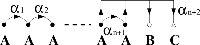
Figure 1: The 7-brane configuration and junctions which realize $SO(2n+4)$.

Now we analyze how the junctions are transformed by the chain of rearrangements of 7-branes that brings ${\bf A}^{n+2}{\bf B}{\bf C}$ into ${\bf A}^{n}{\bf D}^{2}{\bf C}^{2}$. By the Hanany-Witten effect [14, 3] a $[p,q]$-string and a $[r,s]$ 7-brane passing through each other create $(ps-qr)$ $[r,s]$-strings between the two. Hence the string junction which have $n_{1}$ endpoints on $X_{[p,q]}$ and $n_{2}$ on $X_{[r,s]}$ are transformed according to the following identity

$$n_{1}[p,q]+n_{2}[r,s]=n_{2}\left\{[r,s]+(ps-qr)[p,q]\right\}+\left\{n_{1}-(ps-qr)n_{2}\right\}[p,q]$$

in the process of the rearrangement $X_{[p,q]}X_{[r,s]}=X_{[r,s]+(ps-qr)[p,q]}X_{[p,q]}$. Using this formula we find that the junction corresponding to the $\alpha_{i}$ in fig. 1 is transformed to that in fig. 2.

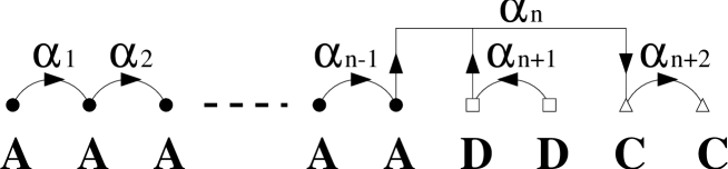
Figure 2: Another representation of the 7-brane configuration and junctions for $SO(2n+4)$.

Once we turn on the $B$ field, the gauge fields corresponding to the junction $\alpha_{j}~{}(n\!\leq\!j\!\leq\!n+2)$ disappear from the massless spectrum. This is because the subgroup $SU(2)$ of the $SO(2n+4)$ which is generated by $\alpha_{j}$ and $-\alpha_{j}$ contains the fluctuation modes that separate the two ${\bf D}$’s or two ${\bf C}$’s. In other words, since the $A_{1}$ singularities cannot be deformed, the scalars corresponding to their deformation parameters cannot have nonzero VEV and must not remain massless. On the other hand, junctions which have the same number of endpoints on each of the two $\bf D$’s (and each of the two $\bf C$’s) remain massless, since they correspond to the fluctuations that move ${\bf D}^{2}$ (and ${\bf C}^{2}$) altogether without breaking them into constituents. By taking these rules into account, we conclude that the massless spectrum representing the simple roots for $Sp(n)$ is generated by $\tilde{\alpha}_{i}\!\equiv\!\alpha_{i}~{}(1\!\leq\!i\!\leq\!n-1)$ and

$$\tilde{\alpha}_{n}\equiv\alpha_{n}+(\alpha_{n}+\alpha_{n+1}+\alpha_{n+2}),$$ (4.5)

as depicted in fig. 3.

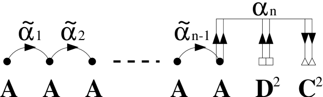
Figure 3: The simple roots for $Sp(n)$.

In particular we can check that $\tilde{\alpha}_{n-1}\cdot\tilde{\alpha}_{n}=-2$ and that the root $\tilde{\alpha}_{n}$ has the norm $(\tilde{\alpha}_{n})^{2}=4$, namely it is a long root. Note that the inner product of the roots is given by minus the intersection number of the corresponding string junctions, i.e. ${\bf J}_{\alpha_{i}}\cdot{\bf J}_{\alpha_{j}}=-\alpha_{i}\cdot\alpha_{j}$ where ${\bf J}_{\alpha_{i}}$ is the junction corresponding to the root $\alpha_{i}$. It is also known that, by compactifying further onto $S^{1}$ and going to the M-theory picture, the intersection number of junctions is identified with that of membranes wrapping on the corresponding two-cycles in $K3$. Furthermore we expect the BPS condition to be unchanged when we turn on the background $B$ field [17]. Thus we can realize $Sp(n)$ gauge group in type IIB string theory by 7-branes and the non-vanishing background $B$ field.

Here we notice that, according to the arguments in [15, 16], the BPS junction ${\bf J}$ have to satisfy

$${\bf J}\cdot{\bf J}=2g-2+b\geq-2,$$ (4.6)

where $g$ and $b$ are, the genus and the number of the boundary, of the corresponding two-cycles in $K3$. Thus it seems impossible to have BPS junctions with self-intersection number $-4$ corresponding to the long roots for $Sp(n)$. However, this is not true because every junction corresponding to the long roots consists of two junctions orthogonal to each other. For example, $\tilde{\alpha}_{n}$ is expressed as the sum of $\alpha_{n}$ and $(\alpha_{n}+\alpha_{n+1}+\alpha_{n+2})$, which would satisfy the BPS condition if the background $B$ field were turned off. Moreover the two junctions are equivalent as cycles of the corresponding $K3$, since under the presence of the $B$ field the $A_{1}$ singularities cannot be deformed. Thus every junction corresponding to a long root is a bound state of two junctions which cannot be separated due to the background $B$ field. Note that when we turn off the $B$ field, it becomes a marginal bound state and can be separated into two BPS junctions.

The 7-brane configuration for $Sp(1)$ has an expression slightly different from the ones for the sequence $Sp(n)~{}(n\geq 2)$. The configuration is given by two pairs of ${\bf D}$ branes, namely ${\bf D}^{2}{\bf D}^{2}$. As pointed out before, this configuration would give $SU(4)$ gauge symmetry if both pairs of ${\bf D}$ branes could be separated. However, we have $Sp(1)$ symmetry here, since the rule concerning massless spectrum allows only one string junction $\alpha$ consisting of two coincident D-strings, which emanate from one of the two ${\bf D}^{2}$’s and get absorbed into the other as depicted in fig. 4. We identify this junction with the simple root for $Sp(1)$.

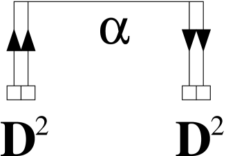
Figure 4: The 7-brane configuration and simple root for $Sp(1)$.

The $O7^{+}$-plane has also been used to produce $Sp(n)$ gauge group, and a certain dual description of CHL string theory contains it [9, 10]. In this description, a modification of the BPS condition of string junction is required [11]. In fact this is same as our result ${\bf J}{\bf J}=-4$ for the long root. The $O7^{+}$-plane might be realized in our picture by eliminating the $B$ field by a singular gauge transformation and localize it to a single point on ${\bf P}^{1}$. By identifying the $O7^{+}$-plane with the point onto which the nonzero $B$ field is localized, we might be able to prove the equivalence between the F-theory with quantized flux and the description with the $O7^{+}$-plane.

5 Conclusions and Discussions

In this paper we have clarified how the $Sp$ type gauge symmetry can be realized in type IIB string theory on ${\bf P}^{1}$ with quantized $B$ flux. In the presence of the $B$ flux the monodromy around the 7-branes are restricted to the subgroup $\Gamma_{0}(2)$ of $SL(2,{\bf Z})$, and due to this condition some 7-branes are forced to be bound together. The analysis of the string junctions on the collapsed 7-branes shows that, by excluding the junctions corresponding to the deformation that would enlarge the monodromy group, we can obtain $Sp(n)$ gauge group out of the $D_{n+2}$ singular fiber. Some junctions in the root system of $Sp(n)$ have the self-intersection $-4$ and at first sight they cannot be BPS saturated. However, a careful look into the corresponding cycles in $K3$ leads us to realize that the long roots always correspond to two degenerate cycles, so that they are BPS saturated.

It would be a very interesting problem to see the full correspondence between the CHL string and type IIB string theory with nonzero $B$ field. To see this, note that the gauge groups of the type (2.8) is possible in the CHL string. However the singular fiber of the type $E_{6}$ or $E_{8}$ is impossible in the type IIB string with the $B$ field, since the monodromies around the corresponding collections of 7-branes are not in $\Gamma_{0}(2)$. In [8] the realization of such gauge groups as well as $Sp(9),Sp(10)$ has been given in a very complicated way. Some enhancements require that the monodromy group become further smaller to the group $\Gamma(2)$. It would be interesting to study how such gauge groups are realized by 7-branes and string junctions in the type IIB string theory.

On the other hand, according to our construction of $Sp$ gauge symmetry the gauge groups of the form $Sp\times Sp$ are apparently possible, which is in contradiction with the result in the CHL string and the description with the $O7^{+}$-plane. In the CHL string we can easily see that one cannot realize the product of $Sp$’s, since by the lemma (2) of section 2 the embedding of the root lattice of $Sp\times Sp$ in $\Gamma_{(2)}$ would result in the embedding of the larger $Sp$ gauge group. Translating this fact into our framework we must conclude that, if we realize two $Sp$ singularity at two different points on ${\bf P}^{1}$ we obtain a large $Sp$ group, with some junctions linking two distant fiber singularities becoming massless. At present we have no idea for resolving this discrepancy.

References

- [1] C. Vafa, Nucl. Phys. B469 (1996) 403, hep-th/9602022.
- [2] D. Morrison and C. Vafa, Nucl. Phys. B473 (1996) 74, hep-th/9602114; Nucl. Phys. B476 (1996) 437, hep-th/9603161.
- [3] O. DeWolfe and B. Zwiebach, Nucl. Phys. B541 (1999) 509, hep-th/9804210.
- [4] A. Johansen, Phys. Lett. B395 (1997) 36, hep-th/9608186.
- [5] M. R. Gaberdiel and B. Zwiebach, Nucl. Phys. B518 (1998) 151, hep-th/9709013.
- [6] S. Chaudhuri, G. Hockney and J.D. Lykken, Phys. Rev. Lett. 75 (1995) 2264, hep-th/9505054.
- [7] S. Chaudhuri and J. Polchinski, Phys. Rev. D52 (1995) 7168, hep-th/9506048.
- [8] M. Bershadsky, T. Pantev and V. Sadov, “F-Theory with Quantized Fluxes”, hep-th/9805056.
- [9] P. Berglund, A. Klemm, P. Mayr and S. Theisen, Nucl. Phys. B558 (1999) 178, hep-th/9805189.
- [10] E. Witten, JHEP 9802 (1998) 006, hep-th/9712028.
- [11] Y. Imamura, JHEP 9907 (1999) 024, hep-th/9905059.
- [12] A. Mikhailov, Nucl. Phys. B534 (1998) 612, hep-th/9806030.
- [13] M. R. Gaberdiel, T. Hauer and B. Zwiebach, Nucl. Phys. B525 (1998) 117, hep-th/9801205.
- [14] A. Hanany and E. Witten, Nucl. Phys. B492 (1997) 152, hep-th/9611230.
- [15] O. DeWolfe, T. Hauer, A. Iqbal and B. Zwiebach, Nucl. Phys. B534 (1998) 261, hep-th/9805220.
- [16] A. Mikhailov, N. Nekrasov and S. Sethi, Nucl. Phys. B531 (1998) 345, hep-th/9803142.
- [17] M. Marino, R. Minasian, G. Moore and A. Strominger, JHEP 0001 (2000) 005, hep-th/9911206.