NSF-ITP-00-37

CITUSC/00-022

hep-th/0005162

EXPONENTIAL HIERARCHY FROM
SPACETIME VARIABLE STRING VACUA

P. Berglund

Institute for Theoretical Physics

University of California, Santa Barbara

Santa Barbara, CA 93106

T. Hübsch^,

Department of Physics and Astronomy

Howard University

Washington, DC 20059

D. Minic

CIT-USC Center for Theoretical Physics

Department of Physics and Astronomy

University of Southern California

Los Angeles, CA 90089-0484

ABSTRACT
It is shown that non-supersymmetric spacetime varying string vacua can lead to an exponential hierarchy between the electroweak and the gravitational scales. The hierarchy is naturally generated by a string coupling of $O(1)$.

1 Introduction

The possibility of our $3{+}1$-dimensional world being a cosmic defect (brane) in a higher-dimensional theory [1, 2, 3, 4, 5, 6, 7, 8, 9, 10, 11, 12] has recently attracted much interest. In particular, the observed hierarchy between the electroweak and the gravitational scales was considered in this context in [11].

In this paper, we show how a class of non-supersymmetric string vacua can naturally lead to an exponential hierarchy. In general we consider $p{+}1$-dimensional cosmic defects embedded in a $D$-dimensional spacetime. These types of models have been considered before in the literature [13, 14, 15, 16]. Here we show explicitly that such cosmic defects emerge as spacetime varying string vacua. The exponential hierarchy between the electroweak and gravitational scales arises from non-trivial warp factors in the metric and naturally is generated by the string coupling of $O(1)$. (The rôle of warp factors in string theory and their relationship to cosmic brane models have been studied in [17, 18, 19, 20].)

Our solutions resemble the stringy cosmic strings  of [21, 22]. The general framework, described in section 2, is that of a higher-dimensional string theory compactified on a Calabi-Yau (complex) $n$-fold, $M_{n}$, some moduli of which are allowed to vary over part of the noncompact space. In the uncompactified Type IIB theory, the rôle of space-dependent moduli is played by the dilaton-axion system, very much like in Vafa’s description of F-theory [23]. The cosmic defect (brane) appears as a singularity of the induced spacetime metric, with its characteristics governed by the energy momentum tensor of the moduli. (In addition, a naked singularity is located at a finite proper distance from the core of the brane.) However, our solutions are non-BPS. This points out to possible stability problems whose detailed study we defer to a future work [24].

The paper is organized as follows: In section 2, we recall the construction of spacetime varying string vacua and generalize the Ansätze of Refs. [21, 22, 23] for the metric; we find non-trivial solutions in which the moduli are non-holomorphic functions over the noncompact space. While this breaks supersymmetry, the exponential warp factors in the metric induce a large hierarchy between the Planck scales in the higher- and lower-dimensional spacetime. In section 3, we study our spacetime-varying dilaton-axion solution when further compactified on a $K3$ or $T^{4}$ to four dimensions, and the generation of an exponential hierarchy. We briefly consider the case of compactifying string theory on a spacetime-varying $K3$, which also gives rise to $3+1$-dimensional vacua with exponential hierarchy. Finally, in section 4, we discuss various possible generalizations of our present work.

2 Spacetime Varying Vacua and Warp Factors

Let us consider compactifications of string theory in which the “internal” space (a Calabi-Yau $n$-fold $M_{n}$) varies over the “observable” spacetime. The parameters of the “internal” space then become spacetime variable moduli fields $\phi^{\alpha}$. The effective action describing the coupling of moduli to gravity of the observable spacetime can be derived by dimensionally reducing the higher dimensional Einstein-Hilbert action [21, 22]. In this procedure one retains the dependence of the Ricci scalar in the gravitational action only on the moduli $\phi^{\alpha}$. Then, the relevant part of the low-energy effective $D$-dimensional action of the moduli of the Calabi-Yau $n$-fold, $M_{n}$, coupled to gravity reads 

$$S_{\rm eff}=\int d^{D}x\sqrt{-g}(-{\textstyle{1\over 2}}R-{\textstyle{1\over 2}}G_{\alpha\bar{\beta}}g^{\mu\nu}\partial_{\mu}\phi^{\alpha}\partial_{\nu}\phi^{\bar{\beta}}+...)~{},$$ (1)

where $\mu,\nu=0,{\cdots},D-1$. We neglect higher derivative terms and set the other fields in the theory to zero as in [21].

We will restrict the moduli to depend on $x_{i}$, $i{=}D{-}2,D{-}1$, so that $\partial_{a}\phi{=}0$, $a{=}0,{\cdots},D{-}3$. The equations of motion are

$$g^{ij}\Big{(}\nabla_{i}\nabla_{j}\phi^{\alpha}+\Gamma^{\alpha}_{\beta\gamma}(\phi,\bar{\phi})\partial_{i}\phi^{\beta}\partial_{j}\phi^{\gamma}\Big{)}=0~{},$$ (2)

and

$$R_{\mu\nu}-{\textstyle{1\over 2}}g_{\mu\nu}R=T_{\mu\nu}(\phi,\bar{\phi})~{},$$ (3)

where the energy-momentum tensor of the moduli is

$$T_{\mu\nu}=-G_{\alpha\bar{\beta}}\Big{(}\partial_{\mu}\phi^{\alpha}\partial_{\nu}\phi^{\bar{\beta}}-{\textstyle{1\over 2}}g_{\mu\nu}\,g^{\rho\sigma}\partial_{\rho}\phi^{\alpha}\partial_{\sigma}\phi^{\bar{\beta}}\Big{)}~{}.$$ (4)

It is useful to define $z\equiv(x_{D-2}+ix_{D-1})$ and rewrite the effective action as

$$S_{\rm eff}=-{\textstyle{1\over 2}}\int d^{D}x~{}\sqrt{-g}\>R-{\textstyle{1\over 2}}\int d^{D-2}x~{}E$$ (5)

where $d^{D-2}x$ refers to the integration measure over the first $D-2$ coordinates, $x_{0},{\cdots},x_{D-3}$. $E$, which we later interpret as the energy density (tension) of the cosmic brane, is given by

$$E\equiv\int d^{2}z\sqrt{-g}~{}G_{\alpha\bar{\beta}}g^{z\bar{z}}\Big{(}\partial_{z}\phi^{\alpha}\partial_{\bar{z}}\phi^{\bar{\beta}}+\partial_{\bar{z}}\phi^{\alpha}\partial_{{z}}\phi^{\bar{\beta}}\Big{)}~{}.$$ (6)

In order to solve the coupled equations of motion for the moduli and gravity, Eqs. (2) and (3), we start with the following Ansatz for the metric

$$ds^{2}=e^{2A(z,\bar{z})}\eta_{ab}dx^{a}dx^{b}+e^{2B(z,\bar{z})}dzd\bar{z}~{}.$$ (7)

This type of Ansatz has appeared recently in various field theory [13, 14], supergravity inspired scenarios [25] and in the context of string theory [26, 27]. The authors in [25] considered the possibility of having a superpotential and hence a potential for the scalar fields. The scalars in our effective action are assumed to be true moduli, with no (super)potential.

Using this Ansatz, Eqs. (2) and (3) produce the following [25]. The ‘$zz$’ Einstein equation leads to ($\partial\equiv\partial_{z}$ and $\bar{\partial}\equiv\partial_{\bar{z}}$)

$$(D{-}2)\Big{[}2\partial A{\partial}B-(\partial A)^{2}-{\partial}^{2}A\Big{]}=2G_{\alpha\bar{\beta}}\partial\phi^{\alpha}{\partial}\phi^{\bar{\beta}}$$ (8)

and the ‘$z\bar{z}$’ Einstein equation becomes

$$(D{-}2)\Big{[}\partial\bar{\partial}A+(D{-}2)\partial A\bar{\partial}A\Big{]}=0.$$ (9)

Note that the ‘$\bar{z}\bar{z}$’ equation is obtained straightforwardly from (8) by replacing $\partial$ by $\bar{\partial}$. We consider the case when $D{>}2$. Then, Eq. (9) lets us simplify the ‘$ab$’ Einstein equation into

$$(D{-}3)\partial\bar{\partial}A+2\partial\bar{\partial}B=-G_{\alpha\bar{\beta}}(\partial\phi^{\alpha}\bar{\partial}\phi^{\bar{\beta}}+\bar{\partial}\phi^{\alpha}{\partial}\phi^{\bar{\beta}})~{}.$$ (10)

Finally, the equation for the moduli reads

$$(D{-}2)\Big{[}2\partial A\bar{\partial}\phi^{\alpha}+2\partial\phi^{\alpha}\bar{\partial}A\Big{]}+4\partial\bar{\partial}\phi^{\alpha}+4G^{\alpha\bar{\gamma}}\frac{\partial G_{\delta\bar{\gamma}}}{\partial\phi^{{\beta}}}\partial\phi^{\beta}\bar{\partial}\phi^{\delta}=0~{}.$$ (11)

Let us start with the well-known supersymmetric solution by requiring that $A{=}0$ and $\bar{\partial}\phi^{\alpha}{=}0$ [21, 22]. Because of holomorphicity, we can simplify the energy density (6). In the case of a variable Calabi-Yau $n$-fold $M_{n}$

$$G_{\alpha\bar{\beta}}\equiv\partial_{\alpha}\partial_{\beta}K,\quad K\equiv-\log{(i^{n}\int\Omega\wedge\bar{\Omega})}~{},$$ (12)

where $\Omega$ is the appropriate holomorphic $n$-form on $M_{n}$. Therefore, Eq. (6) simplifies to

$$E=-i\int\partial\bar{\partial}\log{(i^{n}\int\Omega\wedge\bar{\Omega})}~{}.$$ (13)

Note that $\sqrt{-g}g^{z\bar{z}}=1$ because $A=0$. Finally, one can show that the tension is equal to the deficit angle, $\delta\theta$, caused by the cosmic brane [21, 22]. As expected this saturates the BPS bound,

$$E\geq\delta\theta~{}.$$ (14)

In order to explicitly solve the equations of motion we consider $M_{1}=T^{2}$, fix the Kähler structure and focus on the complex structure modulus, $\tau$, for which the metric on the moduli space is

$$G_{\tau\bar{\tau}}=\frac{-1}{(\tau-\bar{\tau})^{2}}~{}.$$ (15)

This is the case considered in [21]. There, the authors studied a Type II string theory compactified on either a fixed $K3$ or $T^{4}$, followed by a further $T^{2}_{z}$ compactification from six to four dimensions. The subscript $z$ indicates that the torus varies over two ($x_{2,3}$) of the remaining four coordinates, $x_{i},\,i=0,...,3$. When the moduli of $T^{2}_{z}$ depend holomorphically on $z=x_{2}{+}ix_{3}$ cosmic brane solutions with finite energy density which saturate the BPS-bound (14), emerge at particular points in the $z$-plane. Since $\tau=\tau(z)$ Eq. (11) for the modulus $\tau$ is immediately satisfied. The only remaining equation, (10), reads

$$\partial\bar{\partial}(2B)=\partial\bar{\partial}\log{(\tau{-}\bar{\tau})}$$ (16)

which can be explicitly solved and gives rise to the stringy cosmic branes [21].

We are however interested in other solutions for which $A,B{\neq}0$, but still $\bar{\partial}\phi^{\alpha}{=}0$. Although the $\phi^{\alpha}$ are holomorphic, this does not necessarily guarantee that the solution is supersymmetric [26]. (For example, the general analysis of the supersymmetry transformations in $D=10$ type IIB supergravity implies that supersymmetry is broken if the modulus $\tau$, the axion-dilaton system, is non-holomorphic, or the warp factor $A{\neq}0$ [26].) The holomorphicity of $\phi^{\alpha}$ simplifies the equations of motion considerably. In particular, from Eq. (11) we have that moreover $\phi^{\alpha}=$const, and one finds the general solution:

$$e^{2A} = \Big{(}{a(z)+\bar{a}(\bar{z})\over 2a_{0}}\Big{)}^{2\over D-2}~{},$$ (17)

$$e^{2B} = |b_{0}|^{2}\Big{(}{2a_{0}\over a(z)+\bar{a}(\bar{z}))}\Big{)}^{D-3\over D-2}|\partial a(z)|^{2}~{},$$ (18)

where $a_{0}$ and $b_{0}$ are integration constants and $a(z)$ is an arbitrary holomorphic function. Because $\phi^{\alpha}=$const the geometry of the moduli has decoupled. We therefore turn to non-supersymmetric solutions with non-holomorphic moduli. In order to simplify the problem we look for an axially symmetric solution in the plane perpendicular to the cosmic brane. The metric (7) then becomes

$$ds^{2}=e^{2A(\rho)}\eta_{ab}\,dx^{a}dx^{b}+\ell^{2}e^{2\tilde{B}(\rho)}\Big{(}d\rho^{2}+d\theta^{2}\Big{)}~{},$$ (19)

where $z=r_{0}e^{\rho_{0}-\rho+i\theta}$ and $\tilde{B}(\rho)=B(z,\bar{z})-\rho$; the constant parameter $\ell=r_{0}\exp(\rho_{0})$ has dimensions of length. Note that this change of variables corresponds to choosing $a(z)=-\log(z/\ell)$ and $b_{0}=\ell\tilde{b}_{0}$ in Eqs. (17) and (18). The Einstein equations (8)-(10) then become

$$2\Big{[}{\textstyle{D-2\choose 2}}(A^{\prime})^{2}+(D{-}3)A^{\prime\prime}+\tilde{B}^{\prime\prime}\Big{]} = -G_{\alpha\bar{\beta}}(\partial_{\rho}\phi^{\alpha}\partial_{\rho}\phi^{\bar{\beta}}+\partial_{\theta}\phi^{\alpha}\partial_{\theta}\phi^{\bar{\beta}})~{},$$ (20)

$$2(D{-}2)\Big{[}{\textstyle{(D{-}3)\over 2}}(A^{\prime})^{2}+A^{\prime}\tilde{B}^{\prime}\Big{]} = +G_{\alpha\bar{\beta}}(\partial_{\rho}\phi^{\alpha}\partial_{\rho}\phi^{\bar{\beta}}-\partial_{\theta}\phi^{\alpha}\partial_{\theta}\phi^{\bar{\beta}})~{},$$ (21)

$$2(D{-}2)\Big{[}{\textstyle{(D{-}1)\over 2}}(A^{\prime})^{2}+A^{\prime\prime}-A^{\prime}\tilde{B}^{\prime}\Big{]} = -G_{\alpha\bar{\beta}}(\partial_{\rho}\phi^{\alpha}{\partial}_{\rho}\phi^{\bar{\beta}}-\partial_{\theta}\phi^{\alpha}{\partial}_{\theta}\phi^{\bar{\beta}})~{},$$ (22)

while the equation for the moduli (11) reads

$$2(D{-}2)A^{\prime}\partial_{\rho}\phi^{\alpha}+2(\partial^{2}_{\rho}+\partial^{2}_{\theta})\phi^{\alpha}+2G^{\alpha\bar{\gamma}}\frac{\partial G_{\delta\bar{\gamma}}}{\partial\phi^{{\beta}}}(\partial_{\rho}\phi^{\beta}{\partial_{\rho}}\phi^{\delta}+\partial_{\theta}\phi^{\beta}{\partial_{\theta}}\phi^{\delta})=0~{}.$$ (23)

We have used the fact that the two warp factors, $A,\tilde{B}$, in Eq. (19) depend only on $\rho$, and abbreviated $A^{\prime}\equiv\partial_{\rho}{A}$, etc.

To solve these equations we will consider a single modulus scenario, $\phi^{\alpha}{=}\tau$ in which $\tau=a+ie^{-\phi}$, i.e., the axion-dilaton system of the $D{=}10$ Type IIB string theory. The holomorphic solution $\tau=\tau(z)$ is that of $D7$-branes [23]. A more general solution can be obtained along the lines of our earlier analysis. In terms of the $\rho$ and $\theta$ variables we have for non-holomorphic $\tau$ and $A,\tilde{B}\neq 0$ the following solution,

$$e^{2A(\rho)} = ({\rho\over\rho_{0}})^{{2\over D-2}}$$ (24)

$$e^{2\tilde{B}(\rho)} = ({\rho_{0}\over\rho})^{D-3\over D-2}e^{(\rho_{0}^{2}-\rho^{2})/\rho_{0}}~{}.$$ (25)

This is obtained by requiring that $\partial_{\rho}\tau=0$ in (23) .

We find two solutions for $\tau$, depending on whether $\tau$ is purely imaginary or not . Also, note that Eqs. (20)–(23) are unchanged if $\phi^{\alpha}{=}\tau$ is rescaled by a positive multiplicative (normalization) constant. Restricting to $\tau=-\bar{\tau}$, we find the simple particular solution

$$\tau_{I}(\theta)=a_{0}+ig_{0}^{-1}e^{2\sqrt{2}\theta\over\sqrt{\rho_{0}}}~{},\qquad\theta\in[-\pi,\pi]~{}.$$ (26)

Note that when $a_{0}\neq 0$ $\tau_{I}$ satisfies (23) because of the form the metric $G_{\tau\bar{\tau}}$ takes (15). The constants $a_{0}$ and $g_{0}$ are chosen such that rotations through the defining domain of $\theta$ induce an $SL(2,\leavevmode\mathchoice{\hbox{\sf Z\kern-3.99994ptZ}}{\hbox{\sf Z\kern-3.99994ptZ}}{\lower 0.9pt\hbox{\scriptsize\sf Z\kern-2.52ptZ}}{\lower 1.2pt\hbox{\tiny\sf Z\kern-1.8ptZ}})$ action on this solution:

$$\tau_{I}(+\pi)=\frac{a\tau(-\pi))+b}{-\tau_{I}(-\pi)+d}~{}.$$ (27)

With $\tau\neq-\bar{\tau}$, we find the following particular solution

$$\tau_{II}(\theta)=\Big{(}\frac{n}{2}{\textstyle\coth[{2\sqrt{2}\pi\over\sqrt{\rho_{0}}}]}\Big{)}\frac{\pm\sinh[{2\sqrt{2}\theta\over\sqrt{\rho_{0}}}]+i}{\cosh[{2\sqrt{2}\theta\over\sqrt{\rho_{0}}}]}~{},\qquad\theta\in[-\pi,\pi]~{},$$ (28)

where both the axion and the dilaton have a more complicated $\theta$-dependence. Rotations through the defining domain of $\theta$ induce a monodromy action on this solution:

$$\tau_{II}(+\pi)=\tau_{II}(-\pi)\pm n~{}.$$ (29)

Finally, before turning to a more detailed analysis of these solutions, we compute the RR-charge. For (26) the charge is obviously zero as the axion is a constant. This is an indication that this particular cosmic brane is not a $D$-brane . Still, there are certain $D7$-brane configurations whose RR-charge are zero [29]. For (28) we note that when $\rho_{0}>>8\pi^{2}$ we can write the axion as $a\sim\pm n\theta/(2\pi)$ from which we immediately read off the RR-charge as $Q=\pm n$. (In fact, it is easy to show that this holds for all values of $\rho_{0}$.) In this limit we also note that to leading order $\exp(-\phi)=1$. For a fixed $\ell$, i.e., a fixed stress-energy tensor, $\rho_{0}\to\infty$ corresponds to taking $r_{0}\to 0$ and hence the core to zero size (see below for identification of the core in our solution). We thus obtain a situation which is more familiar from that of a $D7$-brane, except for the existence of the singularities at $\rho=0$ and $\rho=\infty$. One may hope that string corrections may render these singularities harmless in such a way that the relation between our solutions and the standard $D7$-branes can be made clearer (see also the discussion in section 3). We will defer a more detailed study of these matters for future work [24].

3 Exponential Hierarchy

In the model considered above, where the dilaton and axion vary over $z{=}x_{8}{+}ix_{9}$, the metric

$$ds^{2}=(\frac{\rho}{\rho_{0}})^{{2\over(D-2)}}\eta_{ab}dx^{a}dx^{b}+\ell^{2}(\frac{\rho_{0}}{\rho})^{{(D-3)\over(D-2)}}e^{(\rho_{0}^{2}-\rho^{2})/\rho_{0}}\Big{(}d\rho^{2}+d\theta^{2}\Big{)}~{},$$ (30)

is identical to that of the global cosmic brane solution studied by the authors of Ref. [13]. They considered a theory with a complex scalar coupled to gravity in which the global $U(1)$ is spontaneously broken. For the particular case of $D=6$ this gives rise to a cosmic 3-brane which naturally can produce an exponential hierarchy between the electroweak and gravitational scales. By compactifying $x_{4},{\cdots},x_{7}$ on a small fixed K3 or a $T^{4}$ in (30), we have thus derived this type of solution from string theory.

Let us now study our solution in more detail following [13]. First, in hindsight it is not too surprising that our solution corresponds to a global cosmic brane. Since the Einstein tensor only depends on $\rho$ while $T_{\mu\nu}$ is independent of $\rho$ they have to be constant in order to satisfy (20)-(22). This is exactly the starting point of the model considered in [13]. The location of the brane is at $\rho=\infty$, which corresponds to $z=0$. (Recall the change of variables in making the ansatz for the metric (19), $|z|=r_{0}e^{\rho_{0}-\rho}$.) However, unlike the supersymmetric case, in which the $D7$-brane is a delta-function source for the stress-energy tensor, the global cosmic brane has finite extent. Roughly speaking the size is that of the location of the core, i.e., $|z|\sim r_{0}$ or $\rho\sim\rho_{0}$. As we will see $\rho_{0}$ (or equivalently $r_{0}$) plays an important role in relating the string coupling to the size of the exponential hierarchy.

Eq. (30) has two (naked) curvature singularities, one at the center of the core, $z=0$ or $\rho=\infty$, and one at $|z|=\ell$ or $\rho=0$. In the latter case the spacetime ends on this naked singularity which is located at a finite proper distance from the core of the brane. According to Ref. [15], one can obtain a different solution by adding a small negative bulk cosmological constant. (This would correspond in our case to a negative correction to the flat potential on the moduli space.) At small distances the solution is that of [13] since the negative contribution to the stress-energy tensor is negligible. However, the effect of the cosmological constant is important at large distances such that the spacetime becomes smooth. In [13] the authors argue that the singularity at $z=0$ is unphysical since the solution does not satisfy the properties of a global cosmic brane; the stress-energy tensor is zero at the center of the core. To completely solve for the global cosmic brane one would have to match the above solution (30) to the metric inside the core and to the metric beyond $|z|=\ell$. Strictly speaking, we cannot claim to have a global cosmic brane solution from string theory until this is done. For now, however, we will not address this issue. We are hopeful that when string corrections are taken into account the singularities will be smoothed out .

We now compute the tension. For both of our two particular solutions, (26) and (28), the integrand in Eq. (6) is ${2\over\rho_{0}^{2}}\rho$. Thus, upon integration from the core to the boundary of spacetime, $0\leq\rho\leq\rho_{0}$, assuming that the contribution from inside the core is finite, small and positive, we find $E=2\pi+O(e^{-\rho_{0}})$. From (30), after changing back to the $z$-variable, it is easy to see that the deficit angle, $\delta\theta=2\pi$. Since $E>\delta\theta$ from Eq. (14) the solution is not BPS. Recall the monodromy outside the core given by Eqs. (27) and (29). These monodromies would in the supersymmetric case correspond to $E_{n}$ and $\hat{E}_{n}$ (the affine extension of $E_{n}$) configurations for $0\leq n\leq 8$  which consist of $n{+}2$ and $n{+}3$ $D7$-branes respectively [29]. However, these configurations cannot account for the deficit angle $\delta\theta=2\pi$. On the other hand, a combination of $n{+}2$ (or $n{+}3$) $D7$-branes placed at one, and $10{-}n$ (or $9{-}n$) $D7$-branes placed at the other singularity can produce the deficit angle of $2\pi$. In fact, the computation of the monodromy around the respective singularities tells us that the charges of these two collections of $D7$ branes should be opposite to each other. This indicates the possibility that the naked singularities could be resolved by replacing them with the above $D7$-branes, subject to the appropriate boundary conditions. In particular, the metric (30) would be matched to the metric of the respective $D7$-brane configurations at $|z|=r_{0}$ and $|z|=\ell$.

As noted above, the solution is by construction non-supersymmetric, and thus it is not in general protected against string corrections. However, the particularly interesting feature of this solution is that the ratio of the $D{-}2$- and $D$-dimensional Planck scales can be naturally large, as in Ref. [13]. Let us therefore briefly review the analysis of [13]. Let $v$ be a new coordinate, $v\equiv v(\rho)$:

$$v=\ell\int_{0}^{\rho}e^{(\rho_{0}^{2}-{\varrho}^{2})/2\rho_{0}}({\rho_{0}\over\varrho})^{{(D-1)\over 2(D-2)}}d\varrho~{}=~{}\ell e^{\rho_{0}/2}\Big{(}{\rho_{0}\over 2}\Big{)}^{3D-5\over 4(D-2)}\textstyle\gamma({D{-}3\over 4(D{-}2)},{\rho^{2}\over 2\rho_{0}})~{},$$ (31)

where $\gamma(\alpha,\xi)\buildrel\rm def\over{=}\int_{0}^{\xi}dt\>e^{-t}t^{\alpha-1}$ is the incomplete (little) gamma-function. Note that we restrict the integration to $0<\rho<\rho_{0}$, i.e., where our solution is valid. Then the metric for our solution reads

$$ds^{2}=({\rho\over\rho_{0}})^{{2\over(D-2)}}\eta_{ab}dx^{a}dx^{b}+({\rho\over\rho_{0}})^{{2\over(D-2)}}dv^{2}+\ell^{2}({\rho_{0}\over\rho})^{{(D-3)\over(D-2)}}e^{(\rho_{0}^{2}-\rho^{2})/\rho_{0}}d\theta^{2}~{}.$$ (32)

To examine the gravitational effects of the cosmic brane one considers metric perturbations of the form

$$ds^{2}=({\rho\over\rho_{0}})^{{2\over(D-2)}}(\eta_{ab}+h_{ab})dx^{a}dx^{b}+({\rho\over\rho_{0}})^{{2\over(D-2)}}dv^{2}+\ell^{2}({\rho_{0}\over\rho})^{{(D-3)\over(D-2)}}e^{(\rho_{0}^{2}-\rho^{2})/\rho_{0}}d\theta^{2}~{}.$$ (33)

After imposing the gauge condition $\partial_{a}h^{ab}=h^{a}_{a}=0$ (see e.g. [12]), we look for solutions of the form

$$h_{ab}=\varepsilon_{ab}e^{ip_{a}x^{a}}e^{in\theta}\frac{\varphi{(v)}}{\psi{(v)}}~{},$$ (34)

where the polarization tensor $\varepsilon_{ab}=$const.,

$$\psi(v(\rho))=\ell^{1/2}e^{(\rho_{0}^{2}-\rho^{2})/4\rho_{0}}(\frac{\rho}{\rho_{0}})^{{D-3\over 4(D-2)}}~{},$$ (35)

and $\eta_{ab}p^{a}p^{b}=-m^{2}$, as in Ref. [13].

The linearized Einstein equation for this type of fluctuations (34) reduces to

$$[-{d^{2}\over dv^{2}}+{1\over\psi}{d^{2}\psi\over dv^{2}}+n^{2}e^{(\rho^{2}-\rho_{0}^{2})/\rho_{0}}({\rho\over\rho_{0}})^{{D-1\over D-2}}]\varphi(v)=m^{2}\varphi(v)~{}.$$ (36)

As shown in Ref. [13], there is one normalizable zero mode ($n=m=0$), which corresponds to $\phi(v)=\psi(v)$, and is well behaved near the singularity. (There is another zero mode which diverges near the singularity, which as argued by the authors of [13], can be eliminated by choosing appropriate boundary conditions. These boundary conditions prevent all conserved quantities from “leaking out” through the boundary.) As pointed out in [13] (see also [31]) the operator on the left-hand side of Eq. (36) for $n=0$ is positive semidefinite, and hence $m^{2}\geq 0$.

Following [13], the existence of a normalizable zero mode allows us to obtain the relation between the four- and six-dimensional Planck scales 

$$M_{4}^{2}=M_{6}^{4}\int\psi^{2}(v)dvd\theta~{}=\pi\ell^{2}e^{\rho_{0}}\rho_{0}^{5/8}\Gamma({\textstyle{3\over 8}})M_{6}^{4}~{}.$$ (37)

If the upper limit of integration is $\rho_{0}$, $\Gamma({\textstyle{3\over 8}})$ should be replaced with $\gamma({\textstyle{3\over 8}},\rho_{0})$; however, the difference quickly becomes negligible if $\rho_{0}>1$. The exponential dependence of $M_{4}/M_{6}$ on $\rho_{0}$ produces an exponential hierarchy, except for small $\rho_{0}$, where (37) reverts to a power-law. Our non-supersymmetric 3-brane solution, derived explicitly from string theory, hence naturally provides for an exponential hierarchy. In addition, the exponential hierarchy is naturally related to a string coupling of $O(1)$. To see this, recall that in our solutions (26) and (28), the dilaton is of the form $\phi=-2\sqrt{2}\theta/\sqrt{\rho_{0}}$. Unless $\rho_{0}$ is very small this means that $\phi\sim\pm O(1)$. In particular, if $\rho_{0}=8\pi^{2}$ then $M_{4}/M_{6}\sim 10^{18}(\ell M_{6})$.

The Fourier $\theta$-expansion in Eq. (34) is now easy to recognize as the Kałuża-Klein mode expansion, especially since it is the $n{=}0$ mode that turns out to correspond to the four-dimensional graviton. The spectrum must be discrete since the volume of the transverse space is finite, and hence the mass gap is $\delta m^{2}\sim M_{6}^{4}/M_{2}^{2}$. (For a more detailed analysis, see appendix A.) Note that although $\delta m^{2}\ll 1$ (in units of $M_{6}^{2}$) the corrections to Newton’s law are of Yukawa potential type and thus exponentially suppressed.

We now turn to the case of a varying K3 compactified string theory. (A varying $T^{4}=T^{2}{\times}T^{2}$ is easy to deal with by iterating the analysis from the previous section.) In this situation, the non-compact spacetime is $D=6$ dimensional. As before, the moduli of the K3 depend on $z{=}x_{5}{+}ix_{6}$ and its conjugate, $\bar{z}$. Rather than studying the full $20$-dimensional moduli space, we will focus on a one-parameter family relevant for discussing $A_{k}$ singularization of a $K3$ surface. In appendix B, the metric is worked out as a function of $t$, the deformation parameter in the defining equation for an $A_{k}$ singularity,

$$XY+U^{k+1}=t(z,\bar{z})~{}.$$ (38)

One can show that, for $|t|<(R^{\prime})^{2}$ (see appendix B), we have

$$\begin{array}[]{rcl}G_{t\bar{t}}&=&\partial_{t}\partial_{\bar{t}}\big{(}-\log(K(t;2))\\[5.69054pt] &=&\Big{(}2R^{\prime 2}|t|^{2k\over k+1}K(t;2)\Big{)}^{-1}+\Big{(}4R^{\prime 4}|t|^{2(k-1)\over k+1}K^{2}(t;2)\Big{)}^{-1}~{}.\end{array}$$ (39)

This is to be compared with the metric on the moduli space in the vicinity of a nodal $T^{2}$, $XY=t(z,\bar{z})$, (see appendix B):

$$\begin{array}[]{rcl}G_{t\bar{t}}&=&\partial_{t}\partial_{\bar{t}}\Big{(}-\log(-\log(t)-\log(\bar{t}))\Big{)}\\[5.69054pt] &=&{[t\bar{t}\log^{2}(t\bar{t})]}^{-1}~{}.\\ \end{array}$$ (40)

As in the case of the $T^{2}$, we then proceed to obtain the equations of motion from the action. We get essentially the same solution, except that the Kähler metric $G_{\alpha\bar{\beta}}$ in (11) is replaced with the one in Eq. (39). Near the location of the singularity, it is enough to keep the leading term. If we consider the solution for which $\partial_{\rho}t=0$, where $\rho=\log r$, $z=re^{i\theta}$ as before, and $t=\bar{t}$, one finds in the limit $t\to 0$

$$\partial^{2}t-\frac{k}{(k+1)}\frac{1}{t}(\partial t)^{2}=0~{}.$$ (41)

This can be compared with the case for the torus

$$\partial^{2}t-\frac{1}{t}(\partial t)^{2}=0~{}.$$ (42)

The particular solution of the type (26) for Eq. (42) is of the form $t=\tilde{c}e^{\tilde{w}\theta}$, while that of (41) is $t=\hat{c}(\theta/(k+1))^{k+1}$. Note that the latter approaches the former when $k\to\infty$. Furthermore, when taking $t\to 0$ we are restricting $t$ to be real because of the way that $t$ is related to $\tau$, as $t\sim\exp(-2\pi\tau_{2})$. The other solution can be dealt with in a similar fashion. It is worth pointing out that in this case one would expect gauge and matter degrees of freedom on the cosmic brane from wrapped $D$-branes on the shrinking cycles.

4 Discussion

To summarize, we have shown in this paper that exponential hierarchy can naturally arise from non-supersymmetric spacetime varying string vacua. The emergence of an exponential hierarchy is naturally related to having the string coupling of $O(1)$ . The four dimensional Planck scale is dynamically determined by the Planck scale in the bulk and the string coupling. In the $D=10$ Type IIB theory, the rôle of space-dependent moduli is played by the dilaton-axion system. This solution, when further compactified on a $K3$ or $T^{4}$, leads to a four dimensional world previously considered only as a phenomenological solution. Note that the emergence of exponential hierarchy without demanding supersymmetry in this particular brane world scenario is akin to the similar phenomenon in technicolor.

There are many realizations of our scheme besides the straightforward compactification on $K3$ or $T^{4}$. For example, iterating non-trivially the above analysis, one might compactify $x_{8},x_{9}$ on a $T^{2}$ and have its complex structure modulus, $\tau$, vary over $z{=}x_{6}{+}ix_{7}$, while its complexified Kähler class, $\varrho$, varies over $w{=}x_{4}{+}ix_{5}$. Each modulus then gives rise to a 5-brane intersecting in a cosmic 3-brane. Another possibility is to have three intersecting 7-branes in $D=10$ type IIB theory, repeating the earlier discussion for the individual 7-branes. Each brane depends on a different transverse complex plane and hence they intersect in a 3-brane .

In all of our scenarios the issue of stability is clearly very important. One possibility is that the non-supersymmetric solutions we have found are unstable and that they decay to a supersymmetric set of $(p,q)$ $D7$-branes. It is natural to expect that certain properties would be preserved in this decay such as the $SL(2,\leavevmode\mathchoice{\hbox{\sf Z\kern-3.99994ptZ}}{\hbox{\sf Z\kern-3.99994ptZ}}{\lower 0.9pt\hbox{\scriptsize\sf Z\kern-2.52ptZ}}{\lower 1.2pt\hbox{\tiny\sf Z\kern-1.8ptZ}})$ monodromy transformation. DeWolfe et al [29] have computed the monodromy for all possible types of $(p,q)$ $D7$-brane configurations. As discussed in section 3, the $E_{n}$ ($\hat{E}_{n}$) and $H_{8-n}$ ($A_{8-n}$) singularities, given by sets of $n{+}2$ ($n{+}3$) and $10{-}n$ ($9{-}n$) isolated $D7$-branes, have monodromies, which coincide with the $SL(2,\leavevmode\mathchoice{\hbox{\sf Z\kern-3.99994ptZ}}{\hbox{\sf Z\kern-3.99994ptZ}}{\lower 0.9pt\hbox{\scriptsize\sf Z\kern-2.52ptZ}}{\lower 1.2pt\hbox{\tiny\sf Z\kern-1.8ptZ}})$ transformations of our $\tau_{I}$ ($\tau_{II}$) solution. This could be taken as an indication that our solutions are longlived excitations around these supersymmetric vacua. One could imagine that the naked singularities in our metric can be resolved in the following manner. After imposing appropriate boundary conditions we patch up the spacetime metric of the supersymmetric solutions with the non-singular part of our metric. The solution obtained in this way would hopefully have the essential features of our solution, i.e., exponential hierarchy. We hope to return to some of these issues in the future [24].

Notice that the warp factors in the expression for the metric that describes our solution depend only on one extra dimension. It seems natural to ask whether there exists a holographic renormalization group [33] interpretation of the bulk equations of motion that describe this brane-world solution.

Finally, it would be interesting to see whether the recent discussion about the possible relaxation mechanisms for the cosmological constant [34] applies to this particular class of string vacua. It would be also interesting to understand whether the conjectured relationship between holography and the cosmological constant problem [35] can be made more specific in this situation.

Acknowledgments: We thank V. Balasubramanian, O. Bergman, R. Corrado, M. Dine, E. Gimon, J. Gomis, P. Hořava, G. Horowitz, T. Imbo, N. Itzhaki, C. Johnson, S. Kachru, P. Mayr, A. Peet, J. Polchinski, E. Silverstein, S. Sethi, K. Sfetsos and S. Thomas for useful discussions. The work of P. B. was supported in part by the National Science Foundation under grant number PHY94-07194. P.B. would like to thank the Caltech/USC Center for Theoretical Physics, as well as Stanford University and University of Durham for their hospitality in the final stages of this project. T. H. wishes to thank the US Department of Energy for their generous support under grant number DE-FG02-94ER-40854 and the Institute for Theoretical Physics at Santa Barbara, where part of this work was done with the support from the National Science Foundation, under the Grant No. PHY94-07194. The work of D. M. was supported in part by the US Department of Energy under grant number DE-FG03-84ER40168. D. M. would like to thank Howard University and the University of Illinois at Chicago for their hospitality while this work was in progress.

Appendix A Potential for massive gravitational modes

In this appendix we analyze the potential, ${\psi^{-1}}d^{2}\psi/dv^{2}$, in the linearized Einstein equation for the gravitational fluctuations (36).

Note that for $\rho\sim 0$, we have the power series expansion [36]

$$v=\ell{\textstyle{1\over 2}}e^{\rho_{0}\over 2}\rho_{0}^{~{}{D-1\over 2(D-2)}}\,\rho^{D-3\over 2(D-2)}\sum_{k=0}^{\infty}{\big{(}{-}\rho^{2}/2\rho_{0}\big{)}^{k}\over k!\Big{(}{D-3\over 2(D-2)}+k\Big{)}}~{},\qquad\rho\sim 0~{},$$ (43)

so that $\psi\approx(\ell v/\rho_{0})^{1/2}$. While an asymptotic formula for $v=v(\rho)$ may be derived for $\rho\to\infty$, it turns out to be less reliable as it involves a formally divergent series.

Since the transcendental change of variables (31) is not invertible in closed form, we are unable to give a $\psi$ as an explicit function of $v$ in closed form. However, using Mathematica’s ParametricPlot, we can plot $\psi$ vs. $v$, and the result is shown in Fig. 1.

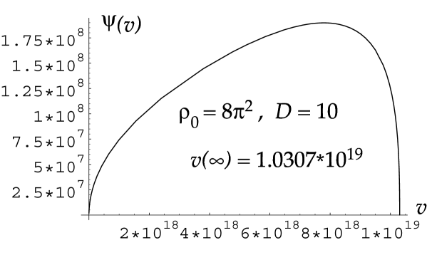
Figure 1: A parametric plot of $\psi(\rho)$, as given in Eq. (31), vs. $v(\rho)$, as given in Eq. (35). Note that $v$ and $v_{\infty}$ are given in units of $\ell$.

Clearly, as a function of $v$, $\psi(v)$ is well approximated by

$$\psi(v;c)\buildrel\rm def\over{=}\sqrt{v}(\frac{v_{\infty}{-}v}{\ell})^{1/c}~{},$$ (44)

for a suitable $c$.

With this approximation, we obtain

$${1\over\psi}{d^{2}\psi\over dv^{2}}\approx-{1/4\over v^{2}}-{1/c\over v(v_{\infty}{-}v)}-{(c{-}1)/c^{2}\over(v_{\infty}{-}v)^{2}}~{},$$ (45)

which is plotted in Fig. 2.

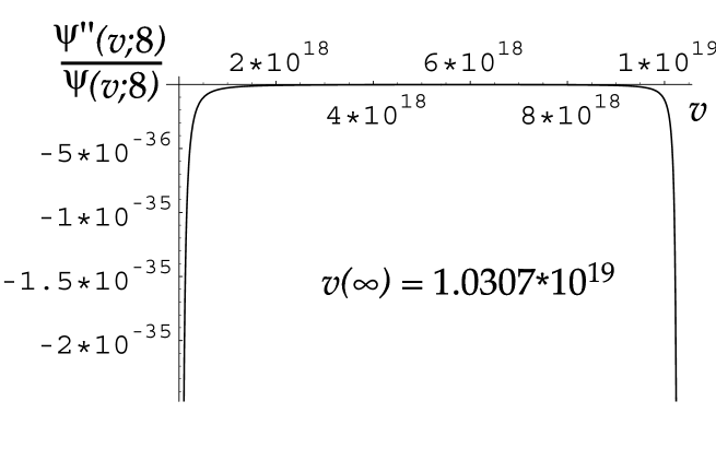
Figure 2: A plot of the potential approximating $\psi^{\prime\prime}/\psi$, as given in Eq. (45), and using $c{=}8$ in Eq. (44). Note that $v$ and $v_{\infty}$ are given in units of $\ell$.

Note that these terms may be thought of as the superposition of two attractive potentials, one at $v{=}0$ and the other at $v{=}v_{\infty}$. The attractive potential at $v{=}0$ (and so $\rho{=}0$, i.e., $|z|=\ell$) corresponds to a naked singularity a finite distance from the core at $\rho=\rho_{0}$ (or $|z|=r_{0}$), while the one at $v_{\infty}$ (i.e., $\rho=\infty$) corresponds to the other singularity at the origin of the $z$-plane.

The approximate potential may well define an exactly soluble quantum mechanical problem. For now, however, let us discuss a further simplification. Firstly, we neglect the middle term in Eq. (45), since it is dominated by the first and the last term, when $v\sim 0$ and $v\sim v_{\infty}$, respectively. Secondly, except for the ‘charge’ of the potential terms, $-{\textstyle{1\over 4}}$ for the first term and $-{c{-}1\over c^{2}}$ for the last, the two terms represent the same type of divergence. Thus we analyze ‘the first half of the potential’, i.e., $V(v)=-{\textstyle{1\over 4\,v^{2}}}$, and look for solutions of the Schrödinger equation

$$\Big{[}-{d^{2}\over dv^{2}}-{1\over 4\,v^{2}}\Big{]}\varphi^{(0)}=m^{2}\varphi^{(0)}~{},$$ (46)

of the form $\varphi^{(0)}(v)=\sqrt{v}f(v)e^{-bv}$. Upon substitution, we find

$$\Big{[}{1\over 4\,v^{2}}-{f^{\prime}\over vf}+{b\over v}-{f^{\prime\prime}\over f}+{2bf^{\prime}\over f}-b^{2}-{1\over 4\,v^{2}}-m^{2}\Big{]}\varphi^{(0)}=0~{}.$$ (47)

This suggests the identification $b=\sqrt{-m^{2}}$: for negative ‘energy’, $m^{2}{<}0$, $b$ is real and the solutions would exponentially decay; for positive ‘energy’, $m^{2}{>}0$, $b$ is imaginary and the solutions would have a plane wave factor. The resulting equation for $f(v)$ then is

$$vf^{\prime\prime}+(1-2bv)f^{\prime}-bf=0~{},$$ (48)

which is easily solved in terms of a power series, $f=\sum_{k=0}^{\infty}c_{k}\,v^{k+s}$. Direct substitution yields

$$0 = \sum_{k=0}^{\infty}c_{k}(k+s)[(k+s-1)+1]v^{k+s-1}-b\sum_{k=0}^{\infty}c_{k}[2(k+s)+1]v^{k+s-1}~{},$$ (49)

$$= c_{0}(s)^{2}v^{s-1}+\sum_{k=0}^{\infty}\Big{\{}c_{k+1}(k+s+1)^{2}-c_{k}b[2(k+s)+1]\Big{\}}v^{k+s}~{}.$$

The vanishing of the coefficient of the first term implies $s{=}0$, and the vanishing of the coefficients for the remaining terms imply the recursion relation:

$$c_{k+1}=c_{k}\,b\>{2(k+s)+1\over(k+s+1)^{2}}~{}.$$ (50)

Since

$${c_{k+1}\,v^{k+1}\over c_{k}\,v^{k}}={2k+1\over(k+1)^{2}}\,bv\to{2bv\over k}<1~{},\quad\mbox{when}\quad k\to\infty~{},$$ (51)

the series defined by the recursion relation (50) converges. Moreover, since large powers of $v$ dominate when $v$ is large, we have that $f(v)\sim e^{2bv}$ when $v$ is large, since the power series of $e^{2bv}$ has the limiting ratio (51). Note that the asymptotically exponential dependence ensures that $v$ equaling a small fraction of $v_{\infty}$ is already sufficiently large for the asymptotic estimate (see Fig. 2). Thus, although the present solution is derived for the simplified toy potential in Eq. (46), it will turn out to be useful both for the full toy model, with the potential (45), and also for the real case, with the potential $\psi^{\prime\prime}/\psi$.

As there is no choice of $b=\sqrt{-m^{2}}$ for which the series would terminate, we conclude that $\varphi^{(0)}(v)=\sqrt{v}f(v)e^{-bv}\sim\sqrt{v}e^{+bv}$ for large $v$. For $m^{2}{<}0$, when $b$ is real and positive, all such solutions are unphysical as they are unnormalizable. (Recall that on retaining only the simple potential as shown in (46), we also let $0\leq v\leq\infty$.) For $m^{2}{>}0$, however, $b$ is imaginary, and $\varphi^{(0)}(v)=\sqrt{v}f(v)e^{-i\beta v}\sim\sqrt{v}e^{i\beta v}$, where $\beta=|b|$. Note in particular that $\varphi^{(0)}(0)\equiv 0$.

Since the potential (45) is qualitatively symmetric with respect to $\{v{=}0\}\leftrightarrow\{v{=}v_{\infty}\}$, we expect to find appropriately ‘reflected’ solutions around the attractive potential at $v{=}v_{\infty}$. Based on the result in the previous case, we also expect $\varphi^{(\infty)}(v)=(v_{\infty}{-}v)^{1/c^{\prime}}g(v)e^{-b(v_{\infty}-v)}$, and in particular that $\varphi^{(\infty)}(v_{\infty})=0$.

Then, the solutions for the full toy potential (45), and also for our actual problem (36) with $n{=}0$, should be well approximated by the linear superpositions $\varphi^{\pm}\buildrel\rm def\over{=}{\textstyle{1\over\sqrt{2}}}(\varphi^{(0)}\pm\varphi^{(\infty)})$. Easily, $\varphi^{\pm}(0)\equiv 0\equiv\varphi^{\pm}(v_{\infty})$—as if there existed impenetrable walls at $v{=}0$ and $v{=}v_{\infty}$. That is, the quantum mechanical problem with the toy potential (45), and also our actual problem (36) with $n{=}0$, behave qualitatively as if the wave-functions $\varphi(v)$ were confined in a (smoothed) infinite potential well. Therefore, we expect a discrete ‘energy’ spectrum $m^{2}{\geq}0$, and a mass gap between $\psi$, the $n{=}0{=}m$ solution of Eq. (36) and the lowest lying state with $m^{2}{>}0$.

Appendix B Kähler Potential Singularities

In this appendix we study the singularities of the Weil-Petersson-Zamolodchikov Kähler potential on the complex structure moduli spaces for several cases of interest. This follows and extends the results of Ref. [37], using the hallmark of Calabi-Yau $n$-folds, $M_{n}$: their covariantly constant and nowhere vanishing $(n,0)$-form. Variations of this $(n,0)$-form describe the complex structure moduli space, in which a codimension-1 subspace (the discriminant locus) corresponds to singular $n$-folds.

B.1 The potential near singularities

Following Ref. [38], the holomorphic $(n,0)$-form may be written as

$$\Omega_{t}={\prod_{i\neq j}dx_{i}\over\phi,_{j}(x;t)}~{},\qquad i,j=1,{\cdots},n{+}1~{}.$$ (52)

Here, $x_{i}$ are local coordinates on the $n{+}1$-fold, $\cal Y$, in which the Calabi-Yau $n$-fold, $M_{n}$, is embedded as the hypersurface $f(x;t)=0$; the $t$ are local coordinates on the (complex structure) moduli space. Generalizations of this to complete intersections of hypersurfaces and other elements of cohomology are straightforward [38, 39].

The integral $K(t;n)\buildrel\rm def\over{=}i^{n}\int_{M_{n}}\overline{\Omega}_{t}{\wedge}\Omega_{t}$ turns out to play a double rôle in the models we consider. Its logarithm is the Kähler potential for the Weil-Petersson-Zamolodchikov metric on the complex structure moduli space [37, 40]. It is also the relative conformal factor in the spacetime metric for the line element transversal to the cosmic $(7{-}2n)$-branes [22]; the peculiar factor, $i^{n}$, ensures the Hermiticity of $K(t;n)$, as necessary for its latter rôle.

As a toy model, compactify the spacetime coordinates $x_{8},x_{9}$ on a $T^{2}$, the complex structure of which is permitted to vary over the space-like $(x_{6},x_{7})$-surface. To this end, $M_{1}=T^{2}$ may be defined as a cubic hypersurface $f(y;t)=0$ in ${\cal Y}=\leavevmode{\rm I\kern-1.79993ptP}^{2}$, the coefficients of which are functions of the moduli, $t$, which in turn are functions of $z{=}x_{8}{+}ix_{9}$ and its conjugate:

$$\begin{array}[]{rcl}f(y;t)&\buildrel\rm def\over{=}&y_{1}^{~{}3}+y_{2}^{~{}3}+y_{3}^{~{}3}-3\,t(z,\bar{z})\,y_{1}y_{2}y_{3}~{}=~{}0~{},\\[5.69054pt] &&(y_{1},y_{2},y_{3})\simeq(\l y_{1},\l y_{2},\l y_{3})~{}.\\ \end{array}$$ (53)

This torus becomes singular ($d_{y}f=0$) at $t_{n}=e^{2n\pi i/3}$, $n=0,1,2$, and $t_{\infty}=\infty$. At each of these points in the $t$-plane, and the corresponding points of the $z$-plane, this highly symmetric torus has three singular points, each of which may be described as a node, i.e., an $A_{1}$ singularity in the classification of Ref. [41]. That is, first change variables in the $t$-plane so that a singularity of Eq. (53) is moved to $t=0$. Then, a holomorphic (but nonlinear) change of local coordinates on $\leavevmode{\rm I\kern-1.79993ptP}^{2}$ turns the defining equation, $f(y;t){=}0$, into $XY=t$, up to higher order terms. For nonzero $t$, the solution of this equation is a rotational hyperboloid. As $t\to 0$, this pinches into a two-sheeted cone with the vertex—the singularity—at $X{=}0{=}Y$. The holomorphic $(1,0)$-form may here be written [38, 37] as

$$\Omega_{t}=f(Y){dY\over Y}~{},\qquad\bar{\partial}_{Y}\,f(Y)=0~{},$$ (54)

this expression being valid within the neighborhood $|X|,|Y|<R$. Furthermore, since $X=t/Y$, we have

$$R>|X|={|t|\over|Y|}~{},\qquad\Rightarrow\qquad|Y|>{|t|\over R}~{},$$ (55)

so that ${|t|\over R}<|Y|<R$, and therefore also $|t|<R^{2}$.

The integral $i\int_{M_{1}}\overline{\Omega}_{t}{\wedge}\Omega_{t}$, as a function of $t$, may then be estimated by dividing the integral into the contributions from each neighborhood in which a singularity develops, and the remaining part which is regular in $t$. The singularities all being equal, locally, we calculate the contribution from the one at $t{=}0$ and multiply by the number of them, $N$. Therefore:

$$K(t;1)\buildrel\rm def\over{=}i\int_{M_{1}}\overline{\Omega}_{t}{\wedge}\Omega_{t}=V_{0}(t)+iN\int_{|t|/R<|Y|<R}\big{|}f(Y)\big{|}^{2}{dY{\wedge}d\bar{Y}\over|Y|^{2}}~{}.$$ (56)

Following Ref. [37], we expand $f(Y)$ in a Taylor series, and note that all the positive powers integrate to regular functions of $t$. We may therefore write

$$i\int_{M_{1}}\overline{\Omega}_{t}{\wedge}\Omega_{t}=V(t)+2N|f_{0}|^{2}\int_{|t|/R<|Y|<R}{d^{2}Y\over|Y|^{2}}~{},$$ (57)

where all the higher order contributions from $[f(Y){-}f_{0}]$ are absorbed in the regular function $V(t)$. Writing $Y=re^{i\theta}$, we easily obtain:

$$\int_{|t|/R<|Y|<R}{d^{2}Y\over|Y|^{2}}=\int_{0}^{2\pi}d\theta\int_{|t|/R}^{R}{rdr\over r^{2}}=2\pi\log\big{(}{R^{2}\over|t|}\big{)}$$ (58)

Upon the transformation $t=R^{2}j(\tau)\sim R^{2}e^{2\pi i\tau}$ near $t=0$, i.e., near $\Im m(\tau)=\infty$,

$$K(t;1)\buildrel\rm def\over{=}i\int_{M_{1}=T^{2}}\overline{\Omega}_{t}{\wedge}\Omega_{t}\propto\Im m(\tau)~{},$$ (59)

which is indeed the standard Kähler potential in the Teichmüller theory .

Before we turn to higher dimensional cases, it is useful to consider the action in terms of the local coordinate $t\propto j(\tau)$. This will facilitate comparison, as we will momentarily see, with the metric for the $A_{k}$ singularities. The Kähler metric in the $t$ coordinate near $t=0$ is given by

$$\begin{array}[]{rcl}G_{t\bar{t}}&=&\partial_{t}\partial_{\bar{t}}\Big{(}-\log[-\log(t)-\log(\bar{t})]\Big{)}\\[5.69054pt] &=&\Big{(}|t|\log|t|^{2}\Big{)}^{-2}~{}.\\ \end{array}$$ (60)

Recall that the metric in terms of the $\tau$ coordinate is given by $G_{\tau\bar{\tau}}=-[\Im m(\tau)]^{-2}$.

We now repeat the calculation of $K(t;2)\buildrel\rm def\over{=}\int_{K3}\Omega_{t}{\wedge}\overline{\Omega}_{t}$, for the Calabi-Yau (complex) 2-folds, the K3 surfaces. The first marked distinction is that there can now be many more types of singularities [41]. Herein, we consider the $A_{k}$ type, for which the defining equation may be brought into the general form

$$XY+U^{k+1}=t(z,\bar{z})~{},$$ (61)

within the neighborhood $|X|,|Y|,|U|^{k+1\over 2}<R$. Solving for $X$, we have that

$$R>|X|={|t-U^{k+1}|\over|Y|}~{},\qquad\Rightarrow\qquad|Y|>{|t-U^{k+1}|\over R}~{},$$ (62)

which gives a lower bound for $|Y|$. The upper bound, $|Y|<R$, then implies through Eq. (62)

$${|t-U^{k+1}|\over R}<|Y|<R~{},\qquad\Rightarrow\qquad|t-U^{k+1}|<R^{2}~{},$$ (63)

which is not guaranteed by $|U|^{k+1\over 2}<R$ when $t{\neq}0$. We thus take $|U|^{k+1\over 2}<R^{\prime}$, where $R^{\prime}$ is sufficiently smaller than $R$. Therefore, with $N$ isolated singular points of the $A_{k}$ type,

$$K(t;2)=V(t)+2N|f_{0}|^{2}\int_{|U|^{k+1\over 2}<R^{\prime}}d^{2}U\int_{|t-U^{k+1}|/R<|Y|<R}{d^{2}Y\over|Y|^{2}}~{}.$$ (64)

The $Y$-integral straightforwardly gives $2\pi\log\big{(}{R^{2}\over|U^{k+1}-t|}\big{)}$, and we are left with the $U$-integral:

$$K(t;2)=V(t)+4\pi N|f_{0}|^{2}\int_{|U|^{k+1\over 2}<R^{\prime}}d^{2}U~{}\log\Big{(}{R^{2}\over|U^{k+1}-t|}\Big{)}~{}.$$ (65)

The result of the $U$-integration depends on whether $|U|^{k+1}<|t|$ or $|U|^{k+1}>|t|$. In the former case, we write

$$|U|^{k+1}<|t|~{}:\qquad\log\big{(}|U^{k+1}-t|\big{)}=\log|t|+\log\Big{|}1-{U^{k+1}\over t}\Big{|}~{},$$ (66)

while in the latter case we write

$$|U|^{k+1}>|t|~{}:\qquad\log\big{(}|U^{k+1}-t|\big{)}=(k{+}1)\log|U|+\log\Big{|}1-{t\over U^{k+1}}\Big{|}~{}.$$ (67)

In both cases, the second logarithm leads to an integral of the general form ($w=\rho e^{i\theta}$)

$$\int_{|w|<C}d^{2}w\log\big{|}1-aw^{b}\big{|}~{},\qquad|aw^{b}|<1~{},$$ (68)

$$= {\textstyle{1\over 2}}\int_{0}^{2\pi}d\theta\int_{0}^{C}\rho d\rho~{}\Big{[}\log(1-a\rho^{b}e^{ib\theta})+\log(1-\bar{a}\rho^{b}e^{-ib\theta})\Big{]}~{},$$

$$= {\textstyle{1\over 2}}\int_{0}^{C}\rho d\rho\int_{0}^{2\pi}d\theta~{}\Big{[}\sum_{n=1}^{\infty}{1\over n}a^{n}\rho^{nb}e^{inb\theta}+\sum_{n=1}^{\infty}{1\over n}\bar{a}^{n}\rho^{nb}e^{-inb\theta}\Big{]}~{}=~{}0~{}.$$

Now, if $R^{\prime}<|t|^{1\over 2}$, then also $|U|^{k+1\over 2}<R^{\prime}<|t|^{1\over 2}$, and we obtain:

$$\int_{|U|^{k+1\over 2}<R^{\prime}}d^{2}U~{}\log\Big{(}{R^{2}\over|U^{k+1}-t|}\Big{)}$$ (69)

$$= \int_{|U|^{k+1\over 2}<R^{\prime}}d^{2}U~{}\bigg{(}\log(R^{2})-\log|t|-\log\Big{|}1-{U^{k+1}\over t}\Big{|}\bigg{)}~{},$$

$$= \pi(R^{\prime})^{4\over k+1}\log\Big{(}{R^{2}\over|t|}\Big{)}~{},\qquad(R^{\prime})^{2}<|t|~{},$$

where we used Eqs. (66) and (68) for the second and the third equality.

On the other hand, if $|t|<(R^{\prime})^{2}$, then for part of the integral $|U|^{k+1\over 2}<|t|^{1\over 2}<R^{\prime}$, and in the remaining part $|t|^{1\over 2}\leq|U|^{k+1\over 2}<R^{\prime}$. Splitting the integration accordingly, we obtain:

$$\int_{|U|^{k+1\over 2}<R^{\prime}}d^{2}U~{}\log\Big{(}{R^{2}\over|U^{k+1}-t|}\Big{)}$$ (70)

$$= \int_{|U|^{k+1\over 2}<R^{\prime}}d^{2}U~{}\log(R^{2})-\int_{|U|^{k+1\over 2}<R^{\prime}}d^{2}U~{}\log\big{|}U^{k+1}-t\big{|}~{},$$

$$= \pi(R^{\prime})^{4\over k+1}\log(R^{2})-\int_{|U|^{k+1\over 2}<|t|^{1\over 2}<R^{\prime}}d^{2}U~{}\bigg{(}\log|t|+\log\Big{|}1-{U^{k+1}\over t}\Big{|}\bigg{)}$$

$$-\int_{|t|^{1\over 2}\leq|U|^{k+1\over 2}<R^{\prime}}d^{2}U~{}\bigg{(}\log|U|^{k+1}+\log\Big{|}1-{t\over U^{k+1}}\Big{|}\bigg{)}~{},$$

$$= 2\pi(R^{\prime})^{4\over k+1}\log(R)-\pi|t|^{2\over k+1}\log|t|-(k{+}1)2\pi\Big{[}{\textstyle{1\over 2}}|U|^{2}\log|U|-{\textstyle{1\over 4}}|U|^{2}\Big{]}_{|t|^{1\over k+1}}^{(R^{\prime})^{2\over k+1}}~{},$$

$$= {\textstyle{k{+}1\over 2}}\pi\Big{(}(R^{\prime})^{4\over k+1}-|t|^{2\over k+1}\Big{)}+2\pi(R^{\prime})^{4\over k+1}\log\Big{(}{R\over R^{\prime}}\Big{)}~{},\quad|t|<(R^{\prime})^{2}~{},$$

where we used Eqs. (66) and (67) in the second, and (68) in the third equality.

To summarize,

$$K(t;2)=V(t)+4\pi^{2}N|f_{0}|^{2}(R^{\prime})^{4\over k+1}I(t;R,R^{\prime})~{},$$ (71)

where $t=t(z,\bar{z})$ and

$$I(t;R,R^{\prime})=\left\{\!\!\!\begin{array}[]{ll}\log\Big{(}{R^{2}\over|t|}\Big{)}~{},&|t|>(R^{\prime})^{2}~{},\\[8.53581pt] {k{+}1\over 2}\Big{[}1-\Big{(}{|t|\over(R^{\prime})^{2}}\Big{)}^{2\over k+1}\Big{]}+2\log\Big{(}{R\over R^{\prime}}\Big{)}~{},{}&|t|<(R^{\prime})^{2}~{},\\ \end{array}\right.$$ (72)

Notice that this function is continuous at $|t|=(R^{\prime})^{k+1}$, albeit not smooth.

References

- [1] V.A. Rubakov and M.E. Shaposhnikov: Phys. Lett. B125(1983)139; ibid. 136.
- [2] M. Visser: Phys. Lett. B159(1985)22; hep-th/9910093.
- [3] I. Antoniadis: Phys. Lett. B246(1990)377.
- [4] M. Gogberashvili: hep-th/9908347.
- [5] P. Hořava and E. Witten: Nucl. Phys. B460(1996)506; Nucl. Phys. B475(1996)94; E. Witten: Nucl. Phys. B471(1996)135.
- [6] T. Hübsch: in Proc. SUSY ’96 Conference, R. Mohapatra and A. Rašin (eds.), Nucl. Phys. (Proc.Supl.) 52A(1997)347–351.
- [7] N. Arkani-Hamed, S. Dimopoulos and G. Dvali: Phys. Lett. B429(1998)263; I. Antoniadis, N. Arkani-Hamed, S. Dimopoulos and G. Dvali: Phys. Lett. B436(1998)257.
- [8] G. Shiu and S.-H. H. Tye: Phys. Rep. D58(1998)106007; Z. Kakushadze and S.-H. H. Tye: Nucl. Phys. B548(1999)180.
- [9] A. Lukas, B.A. Ovrut, K.S. Stelle and D. Waldam: Phys. Rep. D59(1999)086001; for further references see, B.A. Ovrut: hep-th/9905115.
- [10] K.R. Dienes, E. Dudas and T. Gherghetta: Phys. Lett. B436 (1998) 55; Nucl. Phys. B537(1999)47.
- [11] L. Randall and R. Sundrum: Phys. Rev. Lett. 83(1999)3370, hep-th/9905221.
- [12] L. Randall and R. Sundrum: Phys. Rev. Lett. 83(1999)4690, hep-th/9906064.
- [13] A.G. Cohen and D.B. Kaplan: hep-th/9910132; See also, A.G. Cohen and D.B. Kaplan: Phys. Lett. B215(1988)663.
- [14] A. Chodos and E. Poppitz: hep-th/9909199.
- [15] R. Gregory: hep-th/9911015.
- [16] T. Gherghetta and M. Shaposhnikov: hep-th/0004014.
- [17] K. Behrndt and M. Cvetič: hep-th/9909058; hep-th/0001159; M. Cvetič, H. Lu and C.N. Pope: hep-th/0001002; R. Kallosh and A. Linde: hept-th/0001071.
- [18] H. Verlinde: hep-th/9906182; C.S. Chan, P.L. Paul and H. Verlinde: hep-th/0003236.
- [19] B.R. Greene, K. Schalm and G. Shiu: hep-th/0004103.
- [20] P. Mayr: to appear.
- [21] B.R. Greene, A. Shapere, C. Vafa and S.-T. Yau: Nucl. Phys. B337(1990)1.
- [22] P.S. Green and T. Hübsch: Int. J. Mod. Phys. A9(1994)3203–3227.
- [23] C. Vafa: Nucl. Phys. B469(1996)403–418.
- [24] P. Berglund, T. Hübsch and D. Minic: work in progress.
- [25] S.M. Caroll, S. Hellerman and M. Trodden: hep-th/9911083.
- [26] See M.B. Einhorn and L.A. Pando Zayas: hep-th/0003072 for review and references.
- [27] E. Dudas and J. Mourad: hep-th/0004165.
- [28] G. Gibbons, M.B. Green and M.J. Perry: Phys. Lett. B370(1996)37; E. Bergshoeff, M. de Roo, M.B. Green, G. Papadopoulos and P.K. Townsend: Nucl. Phys. B470(1996)113.
- [29] O. DeWolfe, T Hauer, A. Iqbal and B. Zwiebach: hep-th/9812209.
- [30] C.V. Johnson, A.W. Peet and J. Polchinski: hep-th/9911161.
- [31] C. Csáki, J. Erlich, T.J. Hollowood and Y. Shirman: hep-th/0001033.
- [32] W.D. Goldberger and M.B. Wise: hep-ph/9907447.
- [33] See for example, J. de Boer, E. Verlinde and H. Verlinde: hep-th/9912012; V. Balasubramanian, E. Gimon and D. Minic: hep-th/0003147, and references therein.
- [34] N. Arkani-Hamed, S. Dimopoulos, N. Kaloper and R. Sundrum: hep-th/0001197; S. Kachru, M. Schulz and E. Silverstein: hep-th/0001206; J.-W. Chen, M. Luty and E. Pontón: hep-th/0003067.
- [35] T. Banks: hep-th/9601151; E. Verlinde and H. Verlinde: hep-th/9912018; C. Schmidhuber: hep-th/9912156; P. Hořava and D. Minic: hep-th/0001145.
- [36] G. Arfken: Mathematical Methods for Physicists, 3rd ed., (Academic Press, San Diego, 1985).
- [37] P. Candelas, P.S. Green and T. Hübsch: Nucl. Phys. B330(1990)49–102.
- [38] P. Candelas: Nucl. Phys. B298(1988)458.
- [39] P. Berglund and T. Hübsch: Int. J. Mod. Phys. A10(1995)3381–3430.
- [40] P. Candelas, T. Hübsch and R. Schimmrigk: Nucl. Phys. B329(1990)583–590.
- [41] V.I. Arnold, S.M. Gusein-Zade and A.N. Varchenko: Singularities of Differentiable Maps, Vol. I (Birkhäuser, Boston, 1985).