(Anti-)Instantons and
the Atiyah-Hitchin Manifold

Abstract:

The Atiyah-Hitchin manifold arises in many different contexts, ranging from its original occurrence as the moduli space of two $SU(2)$ ’t Hooft-Polyakov monopoles in 3+1 dimensions, to supersymmetric backgrounds of string theory. In all these settings, (super)symmetries require the metric to be hyperkähler and have an $SO(3)$ transitive isometry, which in the four-dimensional case essentially selects out the Atiyah-Hitchin manifold as the only such smooth manifold with the correct topology at infinity. In this paper, we analyze the exponentially small corrections to the asymptotic limit, and interpret them as infinite series of instanton corrections in these various settings. Unexpectedly, the relevant configurations turn out to be bound states of $n$ instantons and $\bar{n}$ anti-instantons, with $|n-\bar{n}|=0,1$ as required by charge conservation. We propose that the semi-classical configurations relevant for the higher monopole moduli space are Euclidean open branes stretched between the monopoles.

1 Introduction

The advent of the now mundane dualities of supersymmetric field and string theories has made it possible to obtain a wealth of non-perturbatively exact results for various couplings in the low-energy effective action of these theories, all of them severely constrained by supersymmetry. In the seminal case of the Coulomb phase of $N=2$ four-dimensional gauge theories [1], the holomorphicity of the prepotential together with electric-magnetic duality was sufficient to fix the dynamics of the vector-multiplets at two-derivative order for all values of the (dimensionally transmuted) gauge coupling $\Lambda^{b_{0}}=\mu^{b_{0}}\exp(-{8\pi^{2}}/{g^{2}_{YM}})$, and the non-perturbative corrections of order $\Lambda^{nb_{0}}e^{in\theta}$ to the one-loop prepotential were identified as the contribution from $n$ Yang-Mills instantons. In a similar manner, exact higher derivative couplings in type I and type II string theories have been obtained from the requirements of S-duality and harmonicity (see [2] for a review and references), and shown to encapsulate the contributions from bound states of arbitrary number $n$ of D-instantons, plus its complex-conjugate series of anti-instanton contributions.

While holomorphy or harmonicity give powerful constraints on the half-BPS–saturated couplings of vector-multiplets of $N=2$ supersymmetry (and presumably any multiplets of higher supersymmetry), the couplings of hypermultiplets are by no means as well understood, even though they occur with the same amount of supersymmetry. The reason is that the hyperkähler or quaternionic constraints on the moduli space of these fields lack a concise and tractable formulation (except perhaps for the twistor methods, which are holomorphic with respect to an auxiliary variable; see [3] for a review). Indeed, there are to date no explicitly known non-homogeneous quaternionic manifolds, and very few explicit examples of hyperkähler manifolds, all of them one-dimensional (in quaternionic units) and with a large number of isometries. Among them are the (multi) Eguchi-Hanson and Taub-NUT gravitational instantons, with asymptotic geometry $\mathbb{R}^{4}/\mathbb{Z}_{k}$ and $\mathbb{R}^{3}\times S^{1}$ respectively, which both possess a triholomorphic $U(1)$ isometry (times $SO(3)$ in the single instanton case; see [4, 5] for a review). Hence, they can be obtained from a harmonic function, which is a sum of a finite number of pole terms in both cases (plus a constant for Taub-NUT). By combining infinite series of poles, it is possible to generate a non-perturbative behaviour, and indeed it was shown by Ooguri and Vafa that such a space describes the quantum-corrected moduli space of the conifold hypermultiplet [6]. In the weak coupling (or asymptotic) limit, one recovers a series of $n$ D-instanton effects, together with its complex-conjugate series of anti-instanton effects, as in the Type IIB case above.

The only explicit example of four-dimensional hyperkähler space without triholomorphic isometry (but with an $SO(3)$ group of “rotational symmetries” not rotating the three Kähler forms) is the Atiyah-Hitchin manifold, first introduced in the context of the moduli space of two BPS monopoles in a 3+1 $SU(2)$ gauge theory with a Higgs field in the adjoint [7]. This space is one-dimensional (after omitting a trivial center-of-mass factor of $\mathbb{R}^{3}\times S^{1}$), and consists of three relative positions of the monopoles (measured in units of the $W$-boson mass $M_{W}=\phi$) and a relative phase $\sigma$. The metric on that space controls the slow motion of the two monopoles [8], which primarily interact through the exchange of massless photons and scalars at long distance [9]. In this regime, the moduli space reduces to a Taub-NUT space, albeit with a negative mass parameter, and hence a singularity at finite distance $r=2$ between the monopoles on the order of the Higgs vev. The metric is independent of the gauge coupling, there are therefore no quantum corrections to this motion, whether perturbative or not. There are however corrections to the long-range interaction due to the exchange of massive $W$-bosons and Higgs field, which dominates when they come close to each other and resolves the singularity. The exact metric was derived in [7] (see also [10]) on the basis of $SO(3)$ isometry and self-duality (which expresses hyperkählerity in 1 dimension), in terms of elliptic functions. The deviation from the Taub-NUT limit is exponentially small in the distance between the monopoles, and is most easily expressed as a deviation to particular components of the Riemann tensor which we shall make precise later,

$$R_{(0)} = \frac{4}{(r-2)^{3}}+\dots$$ (1)

$$R_{(+2)} = \frac{8(-3+9r-6r^{2}+r^{3})}{(r-2)^{2}}e^{-r+i\sigma}+\dots$$ (2)

$$R_{(-2)} = \frac{8(-3+9r-6r^{2}+r^{3})}{(r-2)^{2}}e^{-r-i\sigma}+\dots$$ (3)

where the dots denote subleading corrections of order $e^{-2r}$. The exponential terms in this expression can be interpreted as the semi-classical effect of the Euclidean worldline of a massive $W$-boson stretching between the two monopoles. In the following, we will be mostly interested in the structure of the subleading terms in this expansion, displayed in (18) below, which will reveal the interplay between instantons and anti-instantons.

While the above occurrence of the Atiyah-Hitchin manifold was purely classical, the same manifold arises in many other instances in string or field theory, where the radial parameter $r$ takes another meaning, and in particular can have a coupling-dependent scale. The long distance expansion of the monopole problem then becomes a weak coupling expansion, and the exponentially small corrections can be truly identified with instanton effects. It will be our goal to interpret these effects in the various cases where the Atiyah-Hitchin manifold provides the exact answer, in the hope of drawing lessons for cases where an explicit answer is missing. This program has already been carried out at the one-instanton level in the context of three-dimensional gauge theories [11, 12]: our goal is to extend this study to all higher order non-perturbative contributions, and to other settings where the same effects appear.

The plan of this paper is as follows. We will first review the various instances of the Atiyah-Hitchin manifold in supersymmetric gauge theories, brane constructions and string backgrounds, find the relevant instanton configurations and identify the parameters $r$ and $\sigma$ in these settings. In Section 3, we will revisit the Atiyah-Hitchin metric in a way that allows us to easily extract the series of exponential corrections to the Taub-NUT limit, and identify precisely which instanton configurations contribute to which components of the metric. In Section 4, we shall justify our claim that the exponential corrections arise as contributions from instanton–anti-instanton bound states, and discuss the consequences of this phenomenon for the general question of non-perturbative corrections to hyperkähler manifolds. Some computational details pertaining to Section 3 are relegated to the appendices.

2 Atiyah-Hitchin Manifold, a Festival

In this section, we would like to review some of the many instances of the Atiyah-Hitchin manifold in field or string-theoretic situations, where it provides an exact resummation of all quantum corrections. Being the moduli space of two $SU(2)$ monopoles, it naturally arises whenever we embed monopole solutions in string theory. For a recent discussion on this point see [13]. By duality, it also appears in many other situations where the relevance of monopoles is not immediately obvious. Finally, being a hyperkähler manifold, it appears in many backgrounds with high degree of supersymmetry. Our aim here will be to understand the source of non-perturbative effects, and in particular identify the weight of the semi-classical configurations in terms of the monopole variables (up to factors of 2 and $\pi$, which take care of themselves). In the course of our discussion, we will also mention the occurrence of higher monopole moduli spaces. Even though they are not as well understood as the two $SU(2)$ monopole case, there is yet a considerable amount of knowledge about them which can be carried over to these dual situations.

2.1 Brane lifting of the monopole problem

Much insight into the dynamics of gauge theories has been gained by embedding them into string theory. The monopole problem is no exception, and can be given a simple brane realization. In the limit of far separation, a $k$-monopole configuration of an $SU(2)$ gauge theory is represented by $k$ oriented D-strings stretched between two D3-branes of Type IIB theory. That a D-string ending on a D3-brane acts as magnetic source follows from the worldvolume anomalous coupling $\int F\wedge B_{RR}$ on the D3-brane worldvolume [14]. The four scalars associated to each monopole correspond to the three spatial coordinates of the D1-brane on the D3-brane, together with a fourth scalar $\sigma$ measuring the zero-mode of the U(1) gauge field $\int A$ on the stretched D1-brane world-line.

Figure 1: Worldsheet instanton between two D1-monopoles on a D3-brane worldvolume

Monopoles of $SU(N)$ can be similarly represented as D-strings stretching between different foils of a stack of $N$ D3-branes. Monopoles in 3+1 dimensions can also be lifted to higher extended objects in higher dimensions, or reduced to instantons in 3 dimensions, and so the configuration generalizes to $k$ D$p$-branes stretched between $N$ D$(p+2)$-branes, for $p=0\dots 6$. One virtue of this description is that it makes obvious Nahm’s construction of monopoles, by switching the perspective from the D3-brane to the D1-brane worldvolume: the matrices appearing in Nahm’s equations simply describe the fluctuations of the transverse positions of the D1-branes stretched between the D3-branes [15].

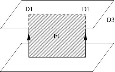
Another virtue of this representation is that it gives a simple geometric representation of the non-perturbative contributions appearing in (1): the value of the Higgs field $\phi$ being related to the distance $L$ between the two D3-branes through $\phi=L/l_{s}^{2}$, the weight $e^{-\phi r}$ simply corresponds to the action of an Euclidean fundamental string stretched between the two D1-branes and D3-branes as depicted on Figure 1. We shall refer to this configuration as a worldsheet instanton. Since the fundamental string stretched between two D3 is the massive $W$-boson of the gauge theory, this rephrases our previous statement that the exponential corrections in (1) come from Euclidean worldlines of $W$-bosons stretching between the two monopoles. The imaginary part $e^{i\sigma}=e^{i(\sigma_{1}-\sigma_{2})}$ of the instanton weight comes from the electric coupling of the boundaries of the fundamental string worldsheet to the U(1) gauge fields $\sigma_{1}$ and $\sigma_{2}$ living on the two D1-branes.

2.2 Monopoles and three-dimensional gauge theories

Figure 2: Duality between monopole moduli space and three-dimensional gauge theory moduli space

The above brane configuration for $p=3$ can be S-dualized to a configuration of $k$ D3-branes stretched between $N$ NS5-branes. This system was studied in detail in [16] as a way of deriving the conjectured equivalence between moduli spaces of monopoles and the Coulomb branch of three-dimensional gauge theories with 8 supersymmetries [17]. Indeed, the theory living on the D3-branes is effectively at distances larger than the 5-brane separation a three-dimensional gauge theory with three Higgs fields in the adjoint (the extra four Higgs fields living on the D3-branes in vacuo are projected out by the boundary conditions imposed by the NS5-branes). In the Coulomb phase, the three-dimensional gauge fields can be dualized into pseudoscalars $\sigma_{i}$, which combine with the three Higgs fields to make $k$ hypermultiplets taking value in some hyperkähler manifold. For $(N,k)=(2,2)$, it was shown on symmetry grounds that the only possibility is the Atiyah-Hitchin manifold [18]. The fact that the moduli space of two $SU(2)$ monopoles appears as the moduli space of the three-dimensional gauge theory is naturally explained from the brane point of view, by simply switching the perspective from the NS5 to the D3-brane worldvolume [16]. More generally, the quantum corrected moduli space of the three-dimensional $SU(k)$ gauge theory is identified with the moduli space of $k$ monopoles in $SU(2)$ [17], and a similar equivalence also holds between moduli spaces of monopoles in ADE gauge groups and Coulomb branches of quiver three-dimensional gauge theories [19].

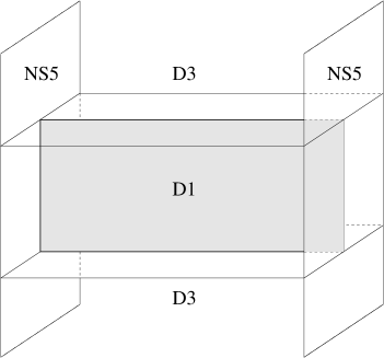
From the point of view of the three-dimensional gauge theory, the $1/(r-2)^{3}$ contribution to the Riemann tensor $R_{(0)}$ appears as a one-loop effect, while the non-perturbative corrections arise as instanton effects from monopoles. This can easily be seen by following the instanton configuration on Figure 1 under S-duality: it becomes an Euclidean D1-brane stretched between both the pair of D3 branes and the pair of NS5-branes, as first discussed in [16] (see Figure 2). From the point of view of the D3-brane, this is an Euclidean monopole, and hence an instanton in the three-dimensional gauge theory. Its classical action is given by $rL/(g_{s}l_{s}^{2})$, where $L=\phi l_{s}^{2}$ is the distance between the D3-branes, and $r$ the distance between the NS5-branes. This can be rewritten in terms of the gauge theory variables as $\phi/g^{2}_{YM}$, which is the appropriate weight for an instanton of the three-dimensional gauge theory. As shown by Polyakov [20], instanton contributions should in addition be weighted by a term $e^{i\sigma}$ where $\sigma$ is the dual of the gauge field in three dimensions, or equivalently the fourth component of the dual magnetic gauge field $A_{m}$ in four dimensions. Indeed, this imaginary part of the action naturally arises from a magnetic coupling $\int A_{m}$ on the D1-brane boundary, dual to the more familiar electric coupling $\int A$ on the fundamental string boundary.

If the moduli space of the $N=4$ three-dimensional gauge theory is really the Atiyah-Hitchin manifold, it should be possible to recover the exponential correction in (1) from a one-instanton computation. This was carried out successfully in [11] for the case without matter, and in [12] for the case with one hypermultiplet, which is conjectured to be described by a double cover of the Atiyah-Hitchin manifold [18]. We will be interested in the extension of these considerations to higher order in the instanton expansion.

2.3 Orientifold Eight-planes with NS5-branes

Figure 3: Left: $SU(2)$ monopoles seen as NS5-branes stuck on an orientifold 8-plane at strong coupling. The instanton corrections come from Euclidean D0-branes stuck on the orientifold. Right: Orientifold 6-plane probed by a D2-brane and its image. The D2-branes are the monopoles of a Higgsed $SU(2)$ and interact by exchange of D0-branes. .

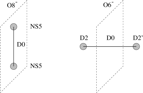
Let us now go back to the case of the D$p$-D$(p+2)$ system, for $p=6$, now embedded in Type I^′. Enhanced $SU(2)$ gauge symmetry occurs when two D8-branes become coincident, but also when the string coupling on one of the $O8^{-}$ orientifold planes becomes infinite. The $SU(2)$ symmetry is Higgsed at finite string coupling, and the massive $W$-bosons are provided by D0-branes stuck on the orientifold plane. It should also be possible to describe $SU(2)$ monopoles on an $O8^{-}$ orientifold at finite coupling. This problem was discussed in [13], where it was shown that the monopoles are NS5-branes stuck on the orientifold plane (see Figure 3 left). These have a relative three- dimensional distance with a phase angle corresponding to the distance between the NS branes in the eleventh direction (string coupling direction). These four scalars form a hypermultiplet which is again parameterizing the AH manifold [13]. The monopoles interact by exchange of $W$-bosons, hence by D0-brane instantons stretched between the two NS5-branes. The non-perturbative corrections to the moduli space are thus suppressed by $\exp[-r/(g_{s}l_{s})]$, where $r$ is the distance between the NS5-branes. This effect is non-perturbative in the string coupling.

2.4 Heterotic string on an ALE space

One can now T-dualize this configuration to a Type I background and further S-dualize to a Heterotic string background. The NS5-branes turn into an $\mathbb{R}^{4}/\mathbb{Z}_{2}$ singularity and the corresponding background is the Heterotic string on $\mathbb{R}^{5,1}\times ALE$, where $ALE$ is the Eguchi-Hanson manifold which resolves the orbifold singularity. The hypermultiplet controlling the size and B-flux of the blown-up two-cycle can be argued to take value again in Atiyah-Hitchin manifold [21]. The origin of the exponential corrections can be traced by following the sequence of dualities, and correspond to world-sheet instantons of the fundamental Heterotic string. This is in agreement with the non-renormalization property of the hypermultiplet moduli space in Heterotic theories with 8 supersymmetries. The exponential corrections are of order $\exp(-A/l_{s}^{2}+iB)$, where $A$ denotes the area of the two-sphere in the blown-up ALE space and $B$ is the B-flux on that cycle. Since these corrections occur purely at string tree-level, it should be possible to recover the exact Atiyah-Hitchin metric in a sigma-model computation. This is however not easy due to the singular nature of the conformal field theory at hand. Note that the identification of Heterotic hypermultiplet spaces and monopole moduli spaces has been generalized in [22, 23].

2.5 D6-branes on $K3$

In a recent series of papers [24, 25, 26] a yet different type of realization of the Atiyah-Hitchin manifold was considered. One looks at a collection of $N$ D6 branes wrapped on a smooth $K3$. The low energy dynamics of these branes is given by a 2+1 dimensional gauge theory with 8 supercharges and gauge group $U(N)$. For the special case of $N=2$ this configuration leads to the gauge theory which was discussed in subsection 2.2 and hence the moduli of the wrapped D6 branes parameterize the Atiyah-Hitchin manifold. The gauge coupling of the 2+1 dimensional theory can be computed to be ${1}/{g_{3}^{2}}=(V_{K3}-l_{s}^{4})/(g_{s}l_{s}^{3})$, where the negative term comes from extrinsic curvature terms on the D6-brane. It vanishes at $V_{K3}=l_{s}^{4}$, which is a point of $SU(2)$ enhanced symmetry in target space (as seen from duality with the Heterotic side for example). The D6-branes can be seen as the monopoles of this broken gauge symmetry in 5+1 dimensions, as they become tensionless at the enhanced symmetry point. The Higgs vev of the three-dimensional gauge theory on the D6-brane is related to the distance $r$ between the 2 D6-branes by $\phi={r}/{l_{s}^{2}}$. The expansion parameter controlling the corrections to the D6-brane moduli space is then $r(V_{K3}-l_{s}^{4})/(g_{s}l_{s}^{5})$. This is also the action of Euclidean D4-branes wrapped on $K3$ and stretching between the D6-branes, which are therefore the relevant instanton configurations. This is consistent with the identification of the wrapped D4-branes as the $W$-bosons of the target-space $SU(2)$ enhanced symmetry. This also identifies the Higgs vev of the target-space gauge symmetry as $(V_{K3}-l_{s}^{4})/(g_{s}l_{s}^{5})$. In fact, the statement made in [24, 25, 26] is slightly different, since it is concerned with the moduli space of a probe D6-brane in the background of a large number $N$ of D6-branes creating a repulson singularity. The claim is that the corrected moduli space is again the Atiyah-Hitchin manifold. The latter then appears as a four-dimensional submanifold of the moduli space of a large number $N$ of $SU(2)$ monopoles.

2.6 Atiyah-Hitchin Backgrounds

An interesting occurrence which is different from all examples discussed above is a string/M-theory background on a manifold which contains the Atiyah-Hitchin manifold, $M_{AH}$. A simple example for such a background is given by M-theory on $\mathbb{R}^{6,1}\times M_{AH}$. This background is known to be the strong coupling dual of Type IIA string theory on $\mathbb{R}^{6,1}\times\mathbb{R}^{3}/I_{3}\times\Omega\times(-1)^{F_{L}}$ or in its more familiar form, an $O6^{-}$ plane [18]. One may argue that D2-brane probes in the vicinity of an orientifold 6-plane behave as monopoles of an Higgsed $SU(2)$ gauge symmetry (see Figure 3, right).

Indeed, the worldvolume theory on a pair of D2-branes is a pure three-dimensional $N=4$ $SU(2)$ theory, and hence has the Atiyah-Hitchin manifold as its moduli space. It should therefore be the case that the singular O6-plane be resolved in the strong string coupling limit into a smooth manifold, the Atiyah-Hitchin manifold itself. In order to relate the Higgs vev to the string parameters, let us consider the gauge theory on the D2-branes. The three dimensional gauge coupling is given by the usual ${1}/{g_{3}^{2}}={l_{s}}/{g_{s}}$. Denote by $r/2$ the distance of the D2 brane to the $O6^{-}$ plane, measured by the $SU(2)$ vev $\phi_{D2}={r}/{l_{s}^{2}}$. The exponential corrections are given by Euclidean D0-branes which are stretched in between the D2 brane and its image with an expansion parameter ${\phi_{D2}}/{g_{3}^{2}}={r}/{g_{s}l_{s}}$. This implies that the $SU(2)$ gauge theory of which the D2-branes are monopoles will have a Higgs vev $\phi_{O6}={1}/{g_{s}l_{s}}$. The enhanced $SU(2)$ symmetry therefore occurs at scale $\phi_{O6}$, which is also the radius of the eleventh dimension. The $W$-bosons of the enhanced $SU(2)$ symmetry are the D0-branes, i.e. the momentum modes of the graviton on the compact eleventh dimension.

3 Atiyah-Hitchin revisited

Having recalled a few occurrences of the Atiyah-Hitchin manifold in string and field theory, and identified what type of non-perturbative corrections it purports to resum, we now would like to extract the precise form of these corrections beyond the one-instanton effect that was displayed in (1). For convenience, we shall use the monopole terminology, but the other cases can be obtained by simply reinterpreting the meaning of the $r$ and $\sigma$ coordinates.

3.1 The Atiyah-Hitchin metric and modular forms

The metric found by Atiyah and Hitchin was originally expressed in terms of elliptic functions, whose appearance is hardly surprising given the fact that the algebraic curve underlying the Nahm equations has genus 1 in the two-monopole case. The asymptotic expansion of elliptic functions is most easily obtained after expressing them in terms of Jacobi Theta functions and other Eisenstein series, whose $q$-expansion is well known. It turns out that the metric can be expressed very concisely in that form, as we now briefly show . We follow the notations and conventions of [9] for the Atiyah-Hitchin metric, and of [28] for modular forms.

The general $SO(3)$ invariant four-dimensional metric can be chosen in the Bianchi IX form,

$$ds^{2}=(abc)^{2}dt^{2}+a^{2}\sigma_{1}^{2}+b^{2}\sigma_{2}^{2}+c^{2}\sigma_{3}^{2}$$ (4)

where $\sigma_{1,2,3}$ are a basis of $SO(3)$-invariant one-forms fulfilling the algebra

$$d\sigma_{i}=\frac{1}{2}\epsilon_{ijk}\sigma_{j}\wedge\sigma_{k}.$$ (5)

An explicit representation for these one-forms is given in terms of the Euler parameterisation of $SU(2)$ as

$$\sigma_{1} = \sin\psi d\theta-\cos\psi\sin\theta d\phi,$$

$$\sigma_{2} = -\cos\psi d\theta-\sin\psi\sin\theta d\phi,$$ (6)

$$\sigma_{3} = d\psi+\cos\theta d\phi$$

The ranges of $\theta$, $\phi$ and $\psi$ are $[0,\pi]$, $[0,2\pi]$ and $[0,2\pi]$ respectively, up to identifications to be discussed below. Requiring the curvature to be self-dual puts three constraints on the coefficients $a,b,c$,

$$\frac{a^{\prime}}{abc}=\frac{b^{2}+c^{2}-a^{2}}{2bc}-\lambda\ ,\ \mbox{etc }$$ (7)

plus the two others obtained by cyclic permutation of $a,b,c$. Here, the prime denotes differentiation with respect to the radial parameter $t$ (see below equation 3.1 for a relation between $r$ and $t$.) and $\lambda$ is an integration constant which is set to 1 in the Atiyah-Hitchin case. Following [7], we define $w_{1}=bc,w_{2}=ca,w_{3}=ab$ to rewrite the differential system as

$$d(w_{1}+w_{2})/dt=-2w_{1}w_{2}\ ,\ \mbox{etc}$$ (8)

known as the Halphen system. Now we observe that Jacobi Theta functions give a simple solution of that system, since they fulfill the modular identity

$$\frac{d}{dt}\left(\frac{\vartheta_{3}^{\prime}}{\vartheta_{3}}+\frac{\vartheta_{4}^{\prime}}{\vartheta_{4}}\right)=\frac{2}{\pi}~{}\frac{\vartheta_{3}^{\prime}}{\vartheta_{3}}\cdot\frac{\vartheta_{4}^{\prime}}{\vartheta_{4}}$$ (9)

where the complex modulus of the Theta function is $\tau=it$ . This implies that a solution of (8) can be chosen as

$$w_{1} = \frac{2}{\pi}\frac{\vartheta_{2}^{\prime}}{\vartheta_{2}}=-\frac{\pi}{6}\left(E_{2}+\vartheta_{3}^{4}+\vartheta_{4}^{4}\right)\$$

$$w_{2} = \frac{2}{\pi}\frac{\vartheta_{3}^{\prime}}{\vartheta_{3}}=-\frac{\pi}{6}\left(E_{2}+\vartheta_{2}^{4}-\vartheta_{4}^{4}\right)\ ,$$ (10)

$$w_{3} = \frac{2}{\pi}\frac{\vartheta_{4}^{\prime}}{\vartheta_{4}}=-\frac{\pi}{6}\left(E_{2}-\vartheta_{2}^{4}-\vartheta_{3}^{4}\right)\ ,$$

which will be shown to satisfy the appropriate boundary conditions. The second equality on the righthand side follows from a standard equality involving the holomorphic Eisenstein series $E_{2}$. Note that $w_{1}<0,w_{2}<0$ and $w_{3}>0$, or equivalently $a>0,b>0,c<0$. The relation to Atiyah and Hitchin’s original formulae is detailed in Appendix A.

The above elliptic functions involve two different asymptotic regimes, $\tau\to i\infty$ and $\tau\to 0$, corresponding to the coincident limit and the large separation limit of the monopoles, respectively. Indeed, as $t\to\infty$, $w_{2}$ and $w_{3}$ become equal and the metric takes the form

$$ds^{2}=4\pi^{2}e^{-2\pi t}\left(\pi^{2}dt^{2}+4e^{-2\pi t}\sigma_{1}^{2}\right)+\frac{\pi}{2}\left(\sigma_{2}^{2}+\sigma_{3}^{2}\right)$$ (11)

up to exponentially small corrections. Changing variables to $\tilde{u}=e^{-\pi t}$, this is recognized as a bolt singularity, which is a mere coordinate singularity if we take the quotient by the symmetry $I_{1}:\theta\to\pi-\theta,\phi\to\phi+\pi,\psi\to-\psi$. The resulting space is a double cover of the Atiyah-Hitchin manifold, the latter being obtained after modding out in addition by $I_{3}:\psi\to\psi+\pi$.

In the $t\to 0$ limit, it is necessary to perform a modular transformation $w_{i}(t)=-\frac{1}{t}-\frac{1}{t^{2}}w_{j}(1/t)$, where $j=3$ for $i=1$; $j=1$ for $i=3$; and $j=2$ for $i=2$. This yields

$$w_{1}(t) = -\frac{1}{t}-\frac{\pi}{t^{2}}(4q+8q^{2}+\dots)\sim-r/\pi$$

$$w_{2}(t) = -\frac{1}{t}+\frac{\pi}{t^{2}}(4q-8q^{2}+\dots)\sim-r/\pi$$ (12)

$$w_{3}(t) = -\frac{1}{t}+\frac{\pi}{t^{2}}(\frac{1}{2}+4q^{2}+\dots)\sim r^{2}(1-2/r)/(2\pi)$$

where $q=e^{-\pi/t}$ and we defined $r=\pi/t$. The first term in $1/t$ arises because of the anomalous modular property of the Eisenstein series $E_{2}$. The Atiyah-Hitchin metric (4) thus reduces to

$$ds^{2}=\frac{1}{2\pi}\left[\left(1-\frac{2}{r}\right)\left(dr^{2}+r^{2}(\sigma_{1}^{2}+\sigma_{2}^{2})\right)+\frac{4}{1-\frac{2}{r}}\sigma_{3}^{2}\right]$$ (13)

where we recognize the Taub-NUT metric with mass parameter $-1$. In particular, the asymptotic geometry is $\mathbb{R}^{3}\times S_{1}$ (mod $\mathbb{Z}_{2}$) and $r$ can be identified as the distance between the monopoles, in units of the $W$-boson mass. The angle $\psi$ parameterizes the circle $S_{1}$ and is the coordinate that we called $\sigma$ before; giving momentum in that direction amounts to giving electric charge to the monopole, turning it into a dyon.

3.2 Four-fermion terms and curvature

We now would like to extract the exponential corrections from the metric described above. For this purpose, we find it convenient to use the language of the three-dimensional $SU(2)$ gauge theory with 8 supercharges. As described in Subsection 2.1, the three Higgs scalars combine with the pseudoscalar $\sigma$ dual to the gauge field in three dimensions to make an hypermultiplet taking values in the Atiyah-Hitchin manifold. The $N=4$ gauge theory has a symmetry group $SU(2)_{H}\times SU(2)_{V}\times SU(2)_{E}$ which is the product of the R-symmetry $SU(2)_{H}$ already present in the six-dimensional $N=1$ theory, the R-symmetry $SU(2)_{V}$ coming from compactification from 6 to 3 dimensions, and the Euclidean group in three dimensions. The fermions transform as $(2,2,2)$ and the bosons as $(1,3+1,1)$, so that $SU(2)_{V}$ is broken to a $U(1)_{V}$ subgroup by the Higgs vev. We choose to align the Higgs field along the “vertical” direction, $\theta=0$.

Given that the theory has 8 supersymmetries, the first quantum corrections arise in the metric of the scalars, or the four-fermion interactions which are related to the former by supersymmetry. It is thus convenient to concentrate on the four-fermion terms, which are contracted with the Riemann tensor of the bosonic moduli space. The antisymmetric product of four fermions transforms as

$$(5,1,1)+(1,5,1)+(1,1,5)+(3,3,3)+(3,3,1)+(3,1,3)+(1,3,3)+(1,1,1)$$

out of which we must keep the singlets under the Euclidean group $SU(2)_{E}$ and the R-symmetry group $SU(2)_{H}$, since the scalars are neutral under them. This only leaves the $(1,5,1)+(1,1,1)$ component.

On the other hand, the Riemann tensor of a hyperkähler manifold transforms as $(1,5,1)$. Indeed, since the Riemann tensor is self-dual, the independent components are $R_{i;j}:=R_{0i0j}$ which make a symmetric tensor of $SU(2)$, and its trace is zero by the cyclic property of the Riemann tensor. It is therefore contracted in the effective action with the $(1,5,1)$ part of the 4 fermion product only. Since the Higgs vev breaks $SU(2)_{V}$ to $U(1)_{V}$, we can split the fluctuations of the three scalars into a complex field $w=x+iy$ of $U(1)_{V}$ charge $++=1$, its complex conjugate $\bar{w}=x-iy$ of $U(1)_{V}$ charge $--=-1$, and a real scalar $z$ of charge $+-=0$. Taking into account the change of basis, the Riemann tensor decomposes into

$$R_{(2)} = R_{++;++}=e^{i\sigma}(R_{1;1}-R_{2;2}+2iR_{1;2})$$

$$R_{(1)} = R_{++;+-}=e^{i\sigma/2}(R_{1;3}+iR_{2;3})$$

$$R_{(0)} = R_{++;--}-R_{+-;+-}=R_{1;1}+R_{2;2}-R_{3;3}$$ (14)

$$R_{(-1)} = R_{--;+-}=e^{-i\sigma/2}(R_{1;3}-iR_{2;3})$$

$$R_{(-2)} = R_{--;--}=e^{-i\sigma}(R_{1;1}-R_{2;2}-2iR_{1;2})$$

These components hence appear in the effective action contracted with the fermion quadrilinears in such a way that the $SU(2)_{H}\times U(1)_{V}\times SU(2)_{E}$ quantum numbers are trivial. In particular, since $\sigma$ enters in the theory only through exponential effects $e^{in\sigma}$, with $n$ integer, it should be the case that $R_{(1)}=R_{(-1)}=0$ exactly, and $R_{(2)}=R_{(-2)}=0$ in perturbation theory. We shall shortly see that this indeed holds.

3.3 The non-perturbative expansion of the Riemann tensor

Having identified the precise components of the Riemann tensor to which instanton effects contribute, we can now proceed to evaluate them using the modular expression of the Atiyah-Hitchin metric. We use the orthonormal basis $e_{0}=abc~{}dt,e_{i}=a_{i}\sigma_{i}$. In terms of the parameters $a,b,c$ entering (4), we find (see Appendix B and [30])

$$R_{1010}=\frac{a^{\prime}}{a(abc)^{2}}\ ,\quad R_{2020}=\frac{b^{\prime}}{b(abc)^{2}}\ ,\quad R_{3030}=\frac{c^{\prime}}{c(abc)^{2}}\ ,\quad R_{i0j0}=0\quad\mbox{if}\quad i\neq j\ .$$ (15)

Using the differential system (7), this can be re-expressed in terms of the $w$’s as

$$R_{1010}=\frac{1}{w_{2}w_{3}}\frac{d}{dt}\left(\frac{(w_{1}w_{3})^{2}+(w_{1}w_{2})^{2}-(w_{2}w_{3})^{2}}{w_{1}^{2}w_{2}w_{3}}\right)\ \mbox{etc.}$$ (16)

and expressed in terms of modular forms using (3.1),

$$R_{1010} = \frac{1}{(E_{2}+e_{3})(E_{2}+e_{4})}\times$$

$$\frac{d}{dt}\left[\frac{E_{2}^{4}+4E_{2}^{3}e_{2}-2E_{2}^{2}(e_{2}^{2}+2e_{3}e_{4})-4E_{2}E_{6}+e_{2}^{4}-(e_{3}e_{4})^{2}-4e_{2}E_{6}}{(E_{2}+e_{2})^{2}(E_{2}+e_{3})(E_{2}+e_{4})}\right].$$

The modular forms $e_{2},e_{3},e_{4}$ are the roots of the polynomial $x^{3}-3E_{4}x-2E_{6}$ and are defined in Appendix A. This result, although not very enlightening, has the virtue of showing that $R_{1;1}$ is a modular form invariant under a $\Gamma^{-}(2)$ subgroup of $Sl(2,\mathbb{Z})$ exchanging $e_{3}$ and $e_{4}$ but leaving $e_{2}$ invariant. Similarly $R_{2;2}$ is invariant under $\Gamma^{0}(2)$ and $R_{3;3}$ under $\Gamma^{+}(2)$, while general modular transformations permute these groups. An important consequence is that $R_{1;1}$ and $R_{2;2}$ have the same $q$-expansion up to alternating signs. Hence the expansion of $R_{(0)}$ only involves even powers, while the expansion of $R_{(\pm 2)}$ only involves odd powers. As we shall see shortly, this is an important consistency check on the interpretation of the result as coming from instanton–anti-instantons bound states.

More precisely, keeping into account the anomalous modular transformation of $w_{i}(t)$, we find that the Riemann tensor has a large distance expansion

$$R_{(0)} = \frac{4}{(r-2)^{3}}-\sum_{n=1}^{\infty}\frac{P_{2n}(r)}{(r-2)^{n+3}}q^{2n}$$ (18)

$$R_{(\pm 2)} = \sum_{n=0}^{\infty}\frac{P_{2n+1}(r)}{(r-2)^{n+2}}q^{2n+1}e^{\pm i\sigma}$$ (19)

where $q=e^{-r}$, and $P_{n}(r)$ is a polynomial of order $3([n/2]+1)$ in $r$ with alternating integer coefficients. The first terms are easily computed using Mathematica,

$$P_{1}(r) = 8(-3+9r-6r^{2}+r^{3})$$

$$P_{2}(r) = 32(6-54r+123r^{2}-124r^{3}+66r^{4}-18r^{5}+2r^{6})$$

$$P_{3}(r) = 32(6-117r+459r^{2}-702r^{3}+495r^{4}-162r^{5}+20r^{6})$$

$$P_{4}(r) = 64(-6+333\ r-2811r^{2}+9023r^{3}-14928r^{4}+14352r^{5}-8392r^{6}+2952r^{7}$$

$$-576r^{8}+48r^{9})$$

The leading $r$ power can be extracted at each order in $q$, yielding

$$R_{(0)} = \frac{2^{2}}{r^{3}}-2^{6}r^{2}q^{2}-3\cdot 2^{10}r^{4}q^{4}-3\cdot 2^{15}r^{6}q^{6}-5\cdot 2^{19}r^{8}q^{8}-3\cdot 7\cdot 2^{22}r^{10}q^{10}+\dots$$

$$R_{(\pm 2)} = e^{\pm i\sigma}\left(2^{3}rq+5\cdot 2^{7}r^{3}q^{3}+5\cdot 2^{13}r^{5}q^{5}+11\cdot 2^{16}r^{7}q^{7}+5\cdot 7\cdot 2^{19}r^{9}q^{9}+\dots\right)$$

Several remarks are in order about these results.

• First, as anticipated in the last section, the perturbative correction only occurs in $R_{(0)}$, as it should be since $U(1)_{V}$ is a symmetry preserved by perturbation theory.

• Second and most importantly, exponential corrections come with an arbitrary power $n$ of the semiclassical weight $q=e^{-r}$, but only with zero-th power of $e^{i\sigma}$ for $n$ even, or first power for $n$ odd. This suggests that the correct interpretation of the non-perturbative exact result is rather a sum of bound states of $n$ instantons and $\bar{n}$ anti-instantons, with overall topological charge $n-\bar{n}=0$ for $R_{(0)}$ and $\pm 1$ for $R_{(\pm 2)}$, as appropriate for charge conservation.

• Third, each power of $q$ comes in with an additional power of $(2r)^{3/2}/(r-2)^{1/2}$, which indicates that the action of the semiclassical configuration is

  $$S_{cl}=(n+\bar{n})\left(r-\frac{1}{2}\log\frac{(2r)^{3}}{r-2}\right)+i(n-\bar{n})\sigma$$ (20)

  This result agrees at large $r$ with the one-instanton result of [11], who found a contribution proportional to $\phi e^{-8\pi^{2}\phi/g_{3}^{2}}$, where the prefactor $\phi$ originates from the one-loop determinant in the instanton background. Our result implies higher loop corrections in the one-instanton background. Besides, it predicts higher order contributions from bound states of instantons and anti-instantons.

• We may have considered instead the near-coincident limit $r\to 0$. The Riemann tensor also admits a $q$-expansion in that regime, with $q=e^{-1/r}$. In fact, this expansion only involves powers of $q$ and not of $r$, since no modular transformation is required, and all coefficients are integer numbers. We do not know of a semi-classical interpretation of this expansion.

This concludes our dissection of the Atiyah-Hitchin metric. The form of the expansion (18) therefore strongly suggests the interpretation of the non-perturbative corrections as contributions of instanton–anti-instanton bound states. We will now try to give further support for this unorthodox claim.

4 Discussion

Half-BPS saturated couplings in supersymmetric string or field theories are commonly thought to satisfy some sort of non-renormalization theorem, restricting them to receive contributions from a limited order in perturbation theory (usually one-loop), as well as exponential corrections coming from half-BPS instantons. This is a well-established fact in a few particular cases, including the prepotential of $N=2$ gauge theories in 4 dimensions, or some higher-derivative terms in string theory. In more general cases, this expectation is based on a simple zero-mode counting argument: an $n$-fermion vertex in the low energy effective action can only receive corrections from instanton configurations with less than $n$ fermionic zero-modes, and hence breaking at most $n$ supersymmetries. This crude argument would seem to rule out contributions from bound states of $N$ BPS instantons, which possess $nN$ zero-modes, but $n(N-1)$ of them are usually lifted by the fermionic interactions in the action governing the collective coordinates. Non-BPS instantons (and in particular superpositions of instantons and anti-instantons) break more supersymmetries, and hence would seem to have too many fermionic zero-modes to make any contribution to the half-BPS couplings.

In the case at hand, we are interested in a four-fermion coupling in a theory with eight supersymmetries. In the language of the three-dimensional gauge theory, the relevant instanton configurations are ’t Hooft-Polyakov monopoles, which have four fermionic zero-modes. In the particular case where the three Higgs fields are aligned (which is automatic in the $SU(2)$ case), the $N$-monopole configurations are in fact exact solutions (in contrast to Yang-Mills instantons in four dimensional gauge theories with a Higgs vev), and hence the $4N$ fermionic zero-modes cannot be lifted. This argument thus predicts contributions from only one BPS monopole to the four-fermion coupling [18]. Our expansion (18) clearly points to a flaw in this line of thought. Indeed, we seem to find contributions from arbitrary numbers of instantons and anti-instantons at the same time, with a net instanton number $n-\bar{n}=0,\pm 1$ . The argument above still correctly predicts the net instanton number, at least when we focus on the particular four-fermion vertex $\psi_{+}\psi_{+}\psi_{+}\psi_{+}$. This is in fact a simple consequence of $U(1)_{V}$ charge conservation, which is violated by $2(n-\bar{n})$ units in a classical background with topological charge $(n-\bar{n})$. An instanton–anti-instanton configuration on the other hand has vanishing topological and hence $U(1)_{V}$ charge, and therefore can be added without disturbing charge conservation.

The argument based on fermionic zero-mode counting can also be evaded. An instanton–anti-instanton configuration does break all supersymmetries, but the action of the supercharges on the instanton configuration does not generate zero-modes of the Dirac operator, since the configuration is not an exact saddle point of the action in the first place. It is in the limit of far separation only, which implies that the fermionic determinant vanishes in the large distance regime in the space of collective coordinates. At finite distance, the number of exact zero-modes is given by the index theorem, which yields $4|n-\bar{n}|$ independent of $n$ and $\bar{n}$ separately . For $|n-\bar{n}|=1$, those are saturated by the four-fermion vertex. We are thus left to evaluate

$$A=\int_{{\cal M}_{(n,\bar{n})}}{\rm Pf}^{\prime}(D)({\det}^{\prime}(\nabla^{2}))^{-1}e^{-S_{cl}+i\sigma(n-\bar{n})}$$ (21)

where ${\cal M}_{(n,\bar{n})}$ denotes the space of bosonic collective coordinates of the $(n,\bar{n})$ instanton–anti-instanton configuration, ${\rm Pf}^{\prime}(D)$ the Pfaffian with the $4|n-\bar{n}|$ zero-modes deleted, and ${\det}^{\prime}(\nabla^{2})$ the bosonic fluctuation determinant with zero-modes deleted. The space of bosonic collective coordinates is not a completely well-defined notion, but makes sense in a dilute gas approximation. The integrand vanishes in the limit of far separation, but can give a finite value from the bulk of the moduli space. In fact, our analysis of the Atiyah-Hitchin metric predicts the value of the integral (21) for any $|n-\bar{n}|=0,1$. It is interesting to note that the total weight in (20) is simply $(n+\bar{n})$ times the weight of an individual instanton (which does receive a logarithmic correction from the quantum fluctuations around it). The effects of the interactions between instantons and anti-instantons are encoded in the polynomial factors appearing in (18), and it would be interesting to analyze them in more detail. In particular, the fact that the coefficients are integer, albeit warranted by the underlying modular symmetry, suggests some topological or counting interpretation of these coefficients.

Figure 4: Bound state of 2 instantons and one anti-instanton stretching between 2 monopoles. The charge across the loop is locally conserved.

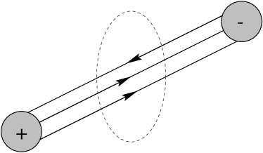
The physical picture that emerges from this discussion is therefore that the exponential corrections to the monopole moduli space arise from semi-classical configurations of $2n+1$ fundamental string world-sheets connecting the two D-strings in the D3-brane setting, or $2n+1$ Euclidean world-lines of $W$-bosons linking the two monopoles. As depicted in Figure 4, $n+1$ of them are oriented in one way and $n$ in the other, so that the total charge cancels (taking into account the net polarization induced by the $\psi_{+}\psi_{+}\psi_{+}\psi_{+}$ vertex). In the three-dimension-al gauge theory language, these are $n+1$ instantons and $n$ anti-instantons occurring at arbitrary Euclidean time.

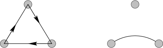
We can ask how this picture generalizes to more than two monopoles, where only the large distance behaviour corresponding to massless exchange is known [31]. Having surmounted the mental barrier of supersymmetry, we suggest that the semi-classical configurations controlling the $n$-SU(2) monopole dynamics are given by strings connecting monopoles in charge-conserving configurations. This includes two-particle interactions as in Figure 4, but also higher point interactions as depicted in Figure 5. Note that in the three-monopole case, the tantalizing $Y$-shaped configuration is not a minimum action configuration, since, due to charge conservation, it is really two $Y$’s with opposite orientations, which prefer to relax into two counter-rotating triangles. Of course, these semi-classical contributions are sub-leading with respect to the power corrections around the two-monopole interactions due to the presence of a third. These have been discussed in [32]. It would be interesting to test our prediction against explicit results for multi-monopoles moduli spaces, as obtained for instance in [33].

Figure 5: Sub-leading semi-classical corrections to the three-monopole moduli space. The two-monopole interaction is modified by the presence of the third.

It is also natural to ask if it is possible to precisely compute the higher-instanton effects in (18) from first principles. Equation (21) is first-principled, but seemingly amenable only to numerical computation. The embedding as a D1-D3 system seems more tractable, but would require some understanding of stacks of fundamental strings with opposite orientations. The NS5-brane setting may also offer some interesting insight, since the instanton is a D-string for which there exists a second quantized description allowing to consider stacks of them (see for instance [34]). The best bet may actually be the Heterotic setting, since the instanton corrections simply arise in that case from world-sheet instantons in the sigma-model $\mathbb{R}^{4}/\mathbb{Z}_{2}$. The latter is unfortunately little understood due to the unresolved singularity. We can however speculate on a possible solution: since the Atiyah-Hitchin metric arises in the decoupling limit of the singularity, one may try to approximate the $\mathbb{R}^{4}/\mathbb{Z}_{2}$ singularity by a $CP^{1}$ sigma-model describing the vanishing two-sphere. Interestingly enough, Cecotti and Vafa have found long ago similar instanton–anti-instanton contributions to the topological-anti-topological fusion coefficients in the $(2,2)$ supersymmetric $CP^{1}$ sigma model [35] (the only example so far of such instanton–anti-instanton effects to our knowledge) . Even more tantalizingly, the $t\bar{t}$ equation controlling the $CP^{1}$ fusion coefficients is nothing but the $SU(2)$ Toda equation [35], while the Atiyah-Hitchin is also known to be controlled by an $SU(\infty)$ Toda equation (see [5] for a review). The study of $(4,0)$ supersymmetric sigma-models may therefore shed an interesting new light on the corrections to hypermultiplet manifolds.

Appendix A From elliptic functions to Theta functions

Atiyah and Hitchin linearize (8) by introducing a solution of the auxiliary equation [7],

$$\frac{d^{2}u}{d\theta^{2}}+\frac{1}{4\sin^{2}\theta}u=0$$ (22)

where $dt/d\theta=1/u^{2}$. Then $w_{1,2,3}$ are given by

$$w_{1} = -u\frac{du}{d\theta}-\frac{1}{2\sin\theta}u^{2}$$

$$w_{2} = -u\frac{du}{d\theta}+\frac{1}{2\tan\theta}u^{2}$$ (23)

$$w_{3} = -u\frac{du}{d\theta}+\frac{1}{2\sin\theta}u^{2}$$

The solution of (22) satisfying the appropriate limits is given by a complete elliptic integral of the first kind,

$$u=\sqrt{2\sin\theta}~{}K\left(\sin\frac{\theta}{2}\right)$$ (24)

where

$$K(k)=\int_{0}^{\pi/2}\frac{d\phi}{\sqrt{1-k^{2}\sin^{2}\phi}}$$ (25)

The region of infinite separation corresponds to $k\to\infty$.

In order to see the equivalence with our solution (3.1), recall that the elliptic integral (25) is naturally associated to an elliptic curve with complex modulus $\tau=iK/K^{\prime}$, where $K^{\prime}=K((1-k^{2})^{1/2})=K(k^{\prime})$ with $k^{\prime}=\cos(\theta/2)$. The relation between $\tau$ and $K,K^{\prime}$ can be rewritten as

$$k=\frac{\vartheta_{2}^{2}}{\vartheta_{3}^{2}}\ ,\quad k^{\prime}=\frac{\vartheta_{4}^{2}}{\vartheta_{3}^{2}}\ ,\quad K=\frac{\pi}{2}\vartheta_{3}^{2}$$ (26)

Expressing the derivative of the elliptic integral $dK/dk=E/(kk^{{}^{\prime}2})-K/k$ in terms of the elliptic integral of the second kind $E(k)$, related to Jacobi Theta functions by

$$E=\frac{\vartheta_{3}^{4}+\vartheta_{4}^{4}}{3\vartheta_{3}^{4}}K+\frac{\pi^{2}}{12K}E_{2}(\tau)=K+\frac{\pi^{2}}{12K}(E_{2}+e_{4})$$ (27)

where we follow the conventions of [28] for modular forms. we find that the solutions (A) can be rewritten as

$$w_{1} = -\frac{\pi}{6}\left(E_{2}+\vartheta_{3}^{4}+\vartheta_{4}^{4}\right)$$

$$w_{2} = -\frac{\pi}{6}\left(E_{2}+\vartheta_{2}^{4}-\vartheta_{4}^{4}\right)$$ (28)

$$w_{3} = -\frac{\pi}{6}\left(E_{2}-\vartheta_{2}^{4}-\vartheta_{3}^{4}\right)$$

which is precisely the same as in (3.1). The line element $d\theta$ can be simply related to $dt$ as $d\theta=-\pi\vartheta_{2}^{2}\vartheta_{4}^{2}dt$, which agrees with the previous relation $dt/d\theta=1/u^{2}$. It is also useful to introduce the modular forms

$$e_{2}=\vartheta_{3}^{4}+\vartheta_{4}^{4}\ ,\quad e_{3}=\vartheta_{2}^{4}-\vartheta_{4}^{4}\ ,\quad e_{4}=-\vartheta_{2}^{4}-\vartheta_{3}^{4}$$ (29)

which are the roots of the Weierstrass polynomial $x^{3}-3E_{4}~{}x-2E_{6}$ and are permuted under modular transformations.

Appendix B Riemann tensor of the Bianchi IX ansatz

Let us now compute the curvature of the Atiyah-Hitchin metric, in the orthonormal basis $e_{0}=abc~{}dt,e_{i}=a_{i}\sigma_{i}$. The Levi-Civita connection is easily found to be

$$\omega_{i0}=a_{i}^{\prime}/(abc)~{}\sigma_{i}\ ,\quad\omega_{jk}=\epsilon_{ijk}(a_{k}^{\prime}/abc+1)~{}\sigma_{k}$$ (30)

and we can compute the curvature through $R=d\omega+[\omega,\omega]$,

$$R_{10}=\frac{d}{dt}\left(\frac{a^{\prime}}{abc}\right)dt\wedge\sigma_{1}+\frac{2abca^{\prime}-(a^{2}+b^{2}-c^{2})b^{\prime}c-(a^{2}+c^{2}-b^{2})bc^{\prime}}{2a^{2}b^{2}c^{2}}\sigma_{2}\wedge\sigma_{3}$$

$$R_{23} = \frac{d}{dt}\left(\frac{b^{2}+c^{2}-a^{2}}{2bc}\right)dt\wedge\sigma_{1}$$

$$-\frac{4b^{\prime}c^{\prime}+bc(a^{2}+b^{2}-c^{2})(a^{2}+c^{2}-b^{2})-2a^{2}bc(b^{2}+c^{2}-a^{2})}{4(abc)^{2}}\sigma_{2}\wedge\sigma_{3}$$

In particular, a necessary condition for the metric to be self-dual is

$$\frac{a^{\prime}}{abc}=\frac{b^{2}+c^{2}-a^{2}}{2bc}-\lambda$$ (32)

which agrees with (7) for $\lambda=1$. Defining $\hat{a}=a^{\prime}/(abc)$, we can rewrite this as

$$R_{10} = R_{23}=\hat{a}^{\prime}dt\wedge\sigma_{1}+(\hat{a}-\hat{b}-\hat{c}-2\hat{b}\hat{c})~{}\sigma_{2}\wedge\sigma_{3}$$

$$R_{20} = R_{31}=\hat{b}^{\prime}dt\wedge\sigma_{2}+(\hat{b}-\hat{c}-\hat{a}-2\hat{c}\hat{a})~{}\sigma_{3}\wedge\sigma_{1}$$ (33)

$$R_{30} = R_{12}=\hat{c}^{\prime}dt\wedge\sigma_{3}+(\hat{c}-\hat{a}-\hat{b}-2\hat{a}\hat{b})~{}\sigma_{1}\wedge\sigma_{2}$$

Using the identity

$$\frac{\hat{a}^{\prime}}{a\cdot abc}=\frac{\hat{a}-\hat{b}-\hat{c}-2\hat{b}\hat{c}}{bc}$$ (34)

we see that the Riemann tensor has the correct symmetry property.

References

- [1] N. Seiberg and E. Witten, “Electric - magnetic duality, monopole condensation, and confinement in N=2 supersymmetric Yang-Mills theory,” Nucl. Phys. B426, 19 (1994) [hep-th/9407087].
- [2] E. Kiritsis, “Duality and instantons in string theory,” in proceedings of the Spring Workshop on Superstrings and Related Matters, Trieste, Italy, March 1999 [hep-th/9906018].
- [3] N. J. Hitchin, A. Karlhede, U. Lindstrom and M. Rocek, “hyperkähler Metrics And Supersymmetry,” Commun. Math. Phys. 108, 535 (1987).
- [4] I. Bakas and K. Sfetsos, “Toda fields of SO(3) hyper-Kähler metrics and free field realizations,” Int. J. Mod. Phys. A12, 2585 (1997) [hep-th/9604003].
- [5] I. Bakas, “Remarks on the Atiyah-Hitchin metric,” Fortsch. Phys. 48, 9 (2000) [hep-th/9903256].
- [6] H. Ooguri and C. Vafa, “Summing up D-instantons,” Phys. Rev. Lett. 77, 3296 (1996) [hep-th/9608079].
- [7] M. F. Atiyah and N. J. Hitchin, “Low-Energy Scattering Of Nonabelian Monopoles,” Phys. Lett. A107, 21 (1985).
- [8] N. S. Manton, “A Remark On The Scattering Of BPS Monopoles,” Phys. Lett. B110, 54 (1982).
- [9] G. W. Gibbons and N. S. Manton, “Classical And Quantum Dynamics Of Bps Monopoles,” Nucl. Phys. B274, 183 (1986).
- [10] M. F. Atiyah and N. J. Hitchin, “The Geometry And Dynamics Of Magnetic Monopoles. M.B. Porter Lectures,” Princeton University Press (1988).
- [11] N. Dorey, V. V. Khoze, M. P. Mattis, D. Tong and S. Vandoren, “Instantons, three-dimensional gauge theory, and the Atiyah-Hitchin manifold,” Nucl. Phys. B502, 59 (1997) [hep-th/9703228].
- [12] N. Dorey, D. Tong and S. Vandoren, “Instanton effects in three-dimensional supersymmetric gauge theories with matter,” JHEP 9804, 005 (1998) [hep-th/9803065].
- [13] A. Hanany and A. Zaffaroni, “Monopoles in string theory,” JHEP 9912, 014 (1999) [hep-th/9911113].
- [14] A. Strominger, “Open p-branes,” Phys. Lett. B383, 44 (1996) [hep-th/9512059].
- [15] D. Diaconescu, “D-branes, monopoles and Nahm equations,” Nucl. Phys. B503, 220 (1997) [hep-th/9608163].
- [16] A. Hanany and E. Witten, “Type IIB superstrings, BPS monopoles, and three-dimensional gauge dynamics,” Nucl. Phys. B492, 152 (1997) [hep-th/9611230].
- [17] G. Chalmers and A. Hanany, “Three dimensional gauge theories and monopoles,” Nucl. Phys. B489, 223 (1997) [hep-th/9608105].
- [18] N. Seiberg and E. Witten, “Gauge dynamics and compactification to three dimensions,” [hep-th/9607163].
- [19] D. Tong, “Three-dimensional gauge theories and ADE monopoles,” Phys. Lett. B448, 33 (1999) [hep-th/9803148].
- [20] A. M. Polyakov, “Quark Confinement And Topology Of Gauge Groups,” Nucl. Phys. B120, 429 (1977).
- [21] A. Sen, “Dynamics of multiple Kaluza-Klein monopoles in M and string theory,” Adv. Theor. Math. Phys. 1, 115 (1998) [hep-th/9707042].
- [22] E. Witten, “Heterotic string conformal field theory and A-D-E singularities,” [hep-th/9909229].
- [23] M. Rozali, “Hypermultiplet moduli space and three dimensional gauge theories,” JHEP 9912, 013 (1999) [hep-th/9910238].
- [24] C. V. Johnson, A. W. Peet and J. Polchinski, “Gauge theory and the excision of repulson singularities,” Phys. Rev. D61, 086001 (2000) [hep-th/9911161].
- [25] L. Jarv and C. V. Johnson, “Orientifolds, M-theory, and the ABCD’s of the enhancon,” [hep-th/0002244].
- [26] C. V. Johnson, “Enhancons, fuzzy spheres and multi-monopoles” [hep-th/0004068].
- [27] L. Takhtajan, “A simple example of modular forms as tau-functions for integrable equations,” Theor. Math. Phys 93 (1993) 1308.
- [28] E. Kiritsis, “Introduction to superstring theory,” Leuven University Press (1998) [hep-th/9709062].
- [29] J. Harnad, J. McKay, “Modular Solutions to Equations of Generalized Halphen Type” [solv-int/9804006].
- [30] J. P. Gauntlett and J. A. Harvey, “S-duality and the dyon spectrum in N=2 superYang-Mills theory,” Nucl. Phys. B463, 287 (1996) [hep-th/9508156].
- [31] G. W. Gibbons and N. S. Manton, Phys. Lett. B356, 32 (1995) [hep-th/9506052].
- [32] C. Fraser and D. Tong, “Instantons, three dimensional gauge theories and monopole moduli spaces,” Phys. Rev. D58, 085001 (1998) [hep-th/9710098].
- [33] C. Houghton, P. W. Irwin and A. J. Mountain, “Two monopoles of one type and one of another,” JHEP 9904, 029 (1999) [hep-th/9902111].
- [34] R. Dijkgraaf, E. Verlinde and H. Verlinde, “Matrix string theory,” Nucl. Phys. B500, 43 (1997) [hep-th/9703030].
- [35] S. Cecotti and C. Vafa, “Exact results for supersymmetric sigma models,” Phys. Rev. Lett. 68, 903 (1992) [hep-th/9111016].