Numerical Analysis of the Double Scaling Limit

in the IIB Matrix Model

S.Horata and H.S.Egawa
^∗,† Theory Division, Institute of Particle and Nuclear Studies,
KEK, High Energy Accelerator Research Organization,
Tsukuba, Ibaraki 305-0801, Japan

^† Department of Physics, Tokai University,
Hiratsuka, Kanagawa 259-1292, Japan

The bosonic IIB matrix model is studied using a numerical method. This model contains the bosonic part of the IIB matrix model conjectured to be a non-perturbative definition of the type IIB superstring theory. The large $N$ scaling behavior of the model is shown performing a Monte Carlo simulation. The expectation value of the Wilson loop operator is measured and the string tension is estimated. The numerical results show the prescription of the double scaling limit.

PACS: 11.25.sq

Keywords: IIB Matrix theory; Numerical analysis; Scaling structure; Area law

1 Introduction

Recent works in string theory have proposed some models as non-perturbative formulations[1, 2, 3]. Especially, the IIB matrix model[2, 3] has been considered as a constructive definition of the type IIB superstring theory. This model is zero-volume limit of the ten-dimensional large $N$ supersymmetric Yang-Mills theory and defined by the following action,

$$S=-\frac{1}{g^{2}}{\rm tr}\left(\frac{1}{4}[A_{\mu},A_{\nu}]^{2}+\frac{1}{2}\bar{\psi}\Gamma^{\mu}[A_{\mu},\psi]\right),$$ (1)

where $A_{\mu}$ and $\psi$ are $N\times N$ traceless Hermitian matrices. The interesting feature of this model is that the space-time coordinates are considered as the eigenvalues of these matrices. Then, we expect that the fundamental issues including the dimensionality and the quantum gravity can be understood by studying the dynamics of the model.

To take the continuum limit ($N\rightarrow\infty$) for the IIB Matrix model, a sensible double scaling limit should be determined dynamically. The scaling property of the model has been studied with the light-cone string field Hamiltonian of the type IIB superstring theory[4]. The scaling property of the two important quantities of the model, the string scale ($\alpha^{\prime}$) and the string coupling constant ($g_{str}$) are determined as follows,

$$\alpha^{\prime} \sim g^{2}N^{a+b}=g^{2}N^{\gamma}\sim Constant,$$

$$g_{str} \sim N^{a-b}.$$ (2)

For the finite value of the string coupling constant ($g_{str}$), one have a restriction, $a=b$. In the IIB matrix model, the exponent ($\gamma$) plays an important role that one can take the large $N$ limit as the continuum limit for the IIB Matrix model. This exponent is determined dynamically.

For studying the dynamical aspects of the model, some Monte Carlo simulations have been performed. In Ref.[5, 6], the existence of the large $N$ limit of bosonic $SU(N)$ Yang-Mills matrix model for $D>2$ has been discussed analytically. Then, in Ref.[7], the bosonic model has been studied with a analytical method, the $1/D$ expansion, as well as a numerical one. The numerical results support the $1/D$ expansion as an effective tool detecting the large $N$ scaling behavior of the model. The leading term of the $1/D$ expansion at $D>3$ suggests that the exponent ($\gamma$) takes a value of 1. We study the model in ten dimensions and reconfirm the expected scaling behavior by a numerical method with a larger size matrix.

In analogy with the two-dimensional model, the Eguchi-Kawai model, we study the scaling property of the Wilson loop in ten-dimensions. The area law of the Wilson loop operator has been found in the four-dimensional model in Ref.[8]. In this article, we also obtain that the area dependence of the Wilson loop obeys the area law in ten dimensions. We calculate the string tension from the area law of the Wilson loop. We thus consider that the scaling property of the string tension is estimated in ten-dimensional model.

This paper is organized as follows. In section 2, we review the model and some perturbative analysis. In section 3, we show the numerical results and the scaling property of the model. Then, we present the data which show the existence of the double scaling limit in the model. Finally, in section 4, we summarize and discuss our numerical results.

2 Large $N$ behavior of correlation functions

First, let us remind the perturbative arguments of the bosonic model and describe briefly the large $N$ behavior of the correlation functions of the gauge fields based on [7].

The bosonic model of the IIB matrix model is given by

$$S_{bosonic}=-\frac{1}{g^{2}}{\rm tr}[A_{\mu},A_{\nu}][A^{\mu},A^{\nu}],$$ (3)

where $A_{\mu}$ are $N\times N$ Hermitian matrices representing the ten-dimensional gauge fields. The coupling constant ($g$) is nothing but a scale parameter and is absorbed with the rescaling of the gauge field ($A_{\mu}$) as $A_{\mu}\rightarrow\frac{1}{\sqrt{g}}A_{\mu}$.

The Schwinger-Dyson equation is given by

$$0=\int dA\frac{\partial}{\partial A}\left({\rm tr}\left(A_{\mu}e^{-S_{bosonic}}\right)\right),$$ (4)

leading to the relation of the correlation function,

$$-<{\rm tr}([A_{\mu},A_{\nu}]^{2})>=D(N^{2}-1)g^{2}.$$ (5)

For the estimation of the large $N$ behavior of the correlation function, $<{\rm tr}([A_{\mu},A_{\nu}]^{2})>$, the matrices ($A_{\mu}$) are decomposed into the diagonal parts ($X_{\mu}^{i}$) and the off diagonal parts ($\tilde{A_{\mu}}^{ij}$), and eq.(5) is taken up to the second order of the off diagonal elements ($\tilde{A_{\mu}}^{ij}$),

$$<{\rm tr}[A_{\mu},A_{\nu}]^{2}>\simeq 2{<{\rm tr}[X_{\mu},\tilde{A}_{\nu}][X_{\mu},\tilde{A}_{\nu}]>-<{\rm tr}[X_{\mu},\tilde{A}_{\nu}][X_{\nu},\tilde{A}_{\mu}]>}.$$ (6)

Counting the order of the diagonal parts, the large $N$ behavior of the leading term of the correlation function counting with the order of the diagonal parts is given by

$$<{\rm tr}[A_{\mu},A_{\nu}]^{2}>\sim g^{2}N^{2}.$$ (7)

For the finite value of the correlation function, an upper limit of the typical scale of the extend of the space-time, for example can be $R^{2}=<{\rm tr}A^{2}>$, is suggested as $R^{2}\leq N^{1/2}$ perturbatively and from the $1/D$ expansion the large $N$ behavior is shown as[7]

$$R^{2}\sim gN^{1/2}.$$ (8)

In the similar manner the correlation functions can be calculated perturbatively.

Next, we consider the Wilson loop operator in the IIB matrix model. The Wilson loop operator and the large $N$ behavior have been studied with the light-cone string field theory of the type IIB superstring[4]. The Wilson loop operator ($w(C)$) is defined as,

$$w(C)={\rm tr}(v(C)),$$ (9)

where $C$ denotes the closed path and $v(C)$ is defined as $v(C)=U_{\mu}\cdots U_{\mu}=P_{C}\exp(i\oint d\sigma k_{\mu}A_{\mu})$ in the bosonic model. The matrices ($U_{\mu}$) are considered as the unitary matrices,

$$U_{\mu}=\exp(i\int dlA_{\mu}).$$ (10)

In the ordinary lattice gauge field theory, the expectation value of the Wilson loop operator which spreads a large area behaves as follows,

$$w(I,J)\sim\exp(-KI\times J),$$ (11)

where $I$ and $J$ are the side lengths of the rectangular loop and $K$ denotes the string tension. In the same analogy, we study the Wilson loop operator of the bosonic model of the IIB matrix model.

From the scaling relation of two-dimensional Eguchi-Kawai model,

$$g^{2}N\sim Constant,$$ (12)

It is expected that the similar scaling relation also holds in the IIB matrix model as[4]

$$\alpha^{\prime}\sim g^{2}N^{\gamma}\sim Constant.$$ (13)

The exponent ($\gamma$) should be determined dynamically from the model. For the large $N$ limit, the parameter ($g^{2}N^{\gamma}$) must be fixed in the IIB matrix model in the same manners as the parameter ($g^{2}N$) must be fixed in the Eguchi-Kawai model.

We notice that the bosonic model is equivalent to the $D>2$ Eguchi-Kawai model in the weak coupling limit. Since the $U(1)^{D}$ symmetry rotates all the eigenvalues by the same angle, the following expansion is valid in the weak coupling region,

$$U_{\mu}\sim e^{i\alpha_{\mu}}e^{iA_{\mu}},$$ (14)

where $\alpha_{\mu}$ take constant values due to the $U(1)^{D}$ symmetry and $A_{\mu}$ are small. The bosonic model action can be obtained by expanding the action of the ten-dimensional Eguchi-Kawai model in terms of $A_{\mu}$. When the higer order terms of $A_{\mu}$ can be neglected, we can obtain the area law of the Wilson loop operator as

$$w(I\times J)=<{\rm tr}(U_{\mu}\cdots U_{\mu})_{I\times J}>\simeq<{\rm tr}(e^{iA_{\mu}}\cdots e^{iA_{\mu}})_{I\times J}>\sim\exp(-K(I\times J)).$$ (15)

In Ref.[8], the area dependence of the Wilson loop operator has been measured and found the area law in $D=4$.

In following section, we will show that the area law holds in the bosonic model of the IIB matrix model in $D=10$.

3 Monte Carlo simulation and Large N behavior of the bosonic model

For numerical simulation of the model, we consider the partition function,

$$Z=\int dAe^{-S_{bosonic}},$$ (16)

where the action $S_{bosonic}$ is given by eq.(3) and the measure of gauge fields is defined by

$$dA=\prod_{\mu=1}^{10}\left[\prod_{i=1}^{N}\prod_{j=i}^{N}d(A_{\mu}^{ij})\right].$$ (17)

The action is quadratic with respect to each component, which means that we can update each component by generating gaussian random number in the heat-bath and the Metropolis algorithm.

To confirm the large $N$ behavior of the model, we measure the following expectation values,

$$R^{2}=<\frac{1}{N}{\rm tr}(A^{2})>,$$

$$<\frac{1}{N}{\rm tr}([A_{\mu},A_{\nu}]^{2})>.$$ (18)

From the perturbative calculation, the large $N$ behaviors are shown as

$$R^{2}\sim gN^{1/2},$$

$$<\frac{1}{N}{\rm tr}([A_{\mu},A_{\nu}]^{2})>\sim g^{2}N.$$ (19)

In Fig.1 and Fig.2, we show the numerical results of the extent of space-time ($R^{2}$) and the correlation function ($<{\rm tr}([A_{\mu},A_{\nu}])^{2}>$) for $D=10$ with $N=16,32,48,64,128$, respectively. We obtain the large $N$ behavior as

$$R^{2}\sim gN^{0.5(1)},$$

$$<\frac{1}{N}{\rm tr}([A_{\mu},A_{\nu}]^{2})>\sim g^{2}N^{-1.0(1))}.$$ (20)

By the simulation using the larger size matrix, the numerical result get close to the expected results.

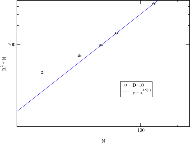
Figure 1: The measurement results of the extent of the space time.

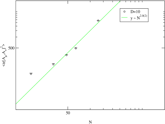
Figure 2: The measurement results of the extent of the correlation function of ($A_{\mu}$).

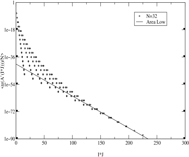
Figure 3: The large area behavior of the Wilson loop operator $w(I\times J)$. Each dot corresponds to different choice of $I$ and $J$.

Then, we consider the Wilson loop operator,

$$w(C)=<\frac{1}{N}{\rm tr}(e^{iA_{\mu}}\cdots e^{iA_{\nu}})>.$$ (21)

We take the loop ($C$) as the rectangular ($I\times J$) where we select any two direction ($\mu,\nu$) in ten dimensions.

We show the measurement results of the loop operator in Fig.3. Since the dependence of the direction of the rectangular is not found, we consider that in the bosonic model the isotropy of the ten-dimensional space-time is not broken down spontaneously.

Then, we calculate the large $N$ behavior by the Wilson loop operator. From the numerical results, the Wilson loop operator, $<\frac{1}{N}{\rm tr}(e^{iA_{\mu}}\cdots e^{iA_{\nu}})_{I\times J}>$, closes to the exponential curve with the large size area. It means that the Wilson loop operator obeys the area law eq.(15).

Then, we can obtain the string tension. In Fig.4, we plot the string tension ($K$).

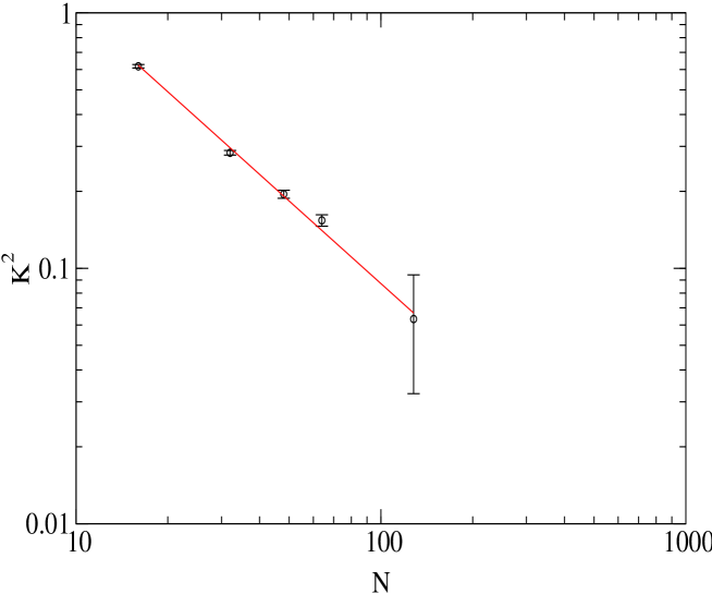
Figure 4: The measurement results of the string tension $a$.

We find the large $N$ behavior of the string tension ($K$),

$$K\sim g^{-2}N^{-1.07(1)}.$$ (22)

From the string tension ($K$), the string scale ($\alpha^{\prime}$) is estimated as

$$\alpha^{\prime}\sim 1/K\sim g^{2}N^{1.07(1)}=Constant.$$

We remark that the string field theory of the light-cone frame suggests[4]

$$\alpha^{\prime}\sim g^{2}N=Constant.$$ (23)

We consider that the numerical result closes to the analytic one and that the four-dimensional model has the same scaling property[8].

Furthermore the numerical result suggests that the large $N$ behavior of the square root of the string tension approximately equal to the inverse of the extent of the space-time.

$$K^{1/2}\sim g^{-1}N^{-0.54(1)}\sim R^{-1}.$$ (24)

It means that the Planck scale of the theory has the same scaling property of the extent of the space time in ten-dimensions. It also holds on the two-dimensional model[9] and the four-dimensional model[8].

4 Summary and Discussion

Let us summarize the main points made in our calculation. We confirm that the Wilson loop operator in the ten-dimensional bosonic model obeys the area law similar to the two and four-dimensional model[9, 8]. For the scaling behavior of the bosonic model of the IIB matrix model, our numerical estimation is

$$\alpha^{\prime}\sim g^{2}N^{1.07(1)}=Constant.$$ (25)

Our results show the ten-dimensional space-time extends with $g^{1/2}N^{0.25(10)}$ and the extent scale of the space-time approximately equal to the Planck scale ($l$), $l\sim K^{-1/2}$. Furthermore, these results are consistent to the suggestion from the string field theory on light-cone frame[4] and the $1/D$ expansion[7]. From the numerical results, we consider that the ten-dimensional bosonic model and the four-dimensional model have the same scaling property.

In this article, we calculate only the bosonic model of the IIB matrix model. For the future work, we are also considering the numerical simulation of the full model including the fermionic term. The supersymmetric four-dimensional model has been studied in Ref.[8]. Optimistically, we expect that we can simplify the fermionic term with the perturbative calculation. In Ref.[10], it is claimed that the model with the 1-loop effective action of the IIB matrix model produces the four-dimensional space-time from the ten-dimensional space-time. We thus make preparations the calculation of the modified model including the fermionic term. The improved supersymmetric model including the fermionic term is studied[11].

Acknowledgements

We would like to thank T.Yukawa, N.Ishibashi, Y.Kitazawa and H.Kawai. Furthermore, we are grateful to F.Sugino, N.Tsuda, S.Oda and especially J.Nishimura for fruitful discussions and advice. We are also grateful to the members of the KEK theory group. Numerical calculations were performed using the NEC SX4 (Tokai University) and the originally designed cluster computer for quantum gravity and strings, CCGS (KEK).

References

- [1] T.Banks, W.Fischler, S.H. Shenker, L.Susskind, Phys. Rev. D55 (1997) 5112, hep-th/9612115.
- [2] N.Ishibashi, H.Kawai, Y.Kitazawa, A.Tsuchiya, Nucl. Phys. B498 (1997) 467, hep-th/9612115.
- [3] H. Aoki, S. Iso, H. Kawai, Y. Kitazawa, T. Tada, A. Tsuchiya, Prog.Theor.Phys.Suppl. 134 (1999) 47.
- [4] M.Fukuma, H.Kawai, Y.Kitazawa, A.Tsuchiya, Nucl. Phys. B510 (1998) 158, hep-th/9705128.
- [5] W.Krauth, H.Nicolai, M.Staudacher, Phys.Lett. B431 (1998) 31, hep-th/9803117.
- [6] W.Krauth, M.Staudacher, Phys.Lett. B435 (1998) 350, hep-th/9804199.
- [7] T.Hotta, J.Nishimura, A.Tsuchiya, Nucl. Phys. B545 (1998) 543, hep-th/9811220.
- [8] J.Ambjørn, K.N.Anagnostopoulos, W.Bietenholz, T.Hotta, J.Nishimura, JHEP 0007 (2000) 013, hep-th/0003208.
- [9] T.Nakajima, J.Nishimura, Nucl.Phys. B528 (1998) 355, hep-th/9802082.
- [10] H.Aoki, S.Iso, H.Kawai, Y.Kitazawa, T.Tada, Prog. Theor. Phys. 99 (1998), 713, hep-th/9802085.
- [11] J.Ambjørn, K.N.Anagnostopoulos, W.Bietenholz, T.Hotta, J.Nishimura, JHEP 0007 (2000) 011, hep-th/0005147.