On the Moduli Space of the Localized 1-5 System

Abstract:

We calculate the effective action for small velocity scattering of localized 1-branes and 5-branes. Momentum is allowed to flow in the direction along the 1-branes so that the moduli space has only 1/8 of the full supersymmetry. Relative to the more familiar case with the 1-branes delocalized along the 5-branes, this introduces new moduli associated with the motion of the 1-branes along the 5-branes. We consider in detail the moduli space metric for the associated two body problem. Even for motion transverse to the 5-brane, our results differ substantially from the delocalized case. However, this difference only appears when both the 1-brane charge and the momentum charge are localized. Despite the fact that, in a certain sense, 1-branes spontaneously delocalize near a 5-brane horizon, the moduli space metric in this limit continues to differ from the delocalized result. This fact may be of use in developing a new description of the associated BPS bound states. The new terms depend on the torus size $L$ in such a way that they give a finite contribution in the $L\rightarrow\infty$ limit.

1 Introduction

Brane moduli spaces, in particular those of black hole configurations, have been investigated extensively over the last few years [1, 2, 3, 4, 5, 6, 7, 8]. One motivation is that in various limits such moduli spaces should be related to the ADS/CFT conjecture [9, 10]. In particular, recent work [5, 11, 12] has focused on cases connected to the elusive relation between $1+1$ ADS space and a $0+1$ CFT.

A closely related motivation of [5, 11, 12] is the attempt to understand the internal states of black holes in terms of the multi-black hole moduli space. In contrast to the description used in [13] to account for the entropy of such black holes, this new description could be valid in a regime of couplings more properly associated with large classical black holes. Such a description could then lead to better insight into the nature of black hole internal states.

Since in M-theory the black holes themselves are believed to be marginally bound states of various types of branes, one might expect the full moduli space associated with the constituent branes to be relevant to this problem. After all, if states in the near horizon limit of the multi-black hole moduli space are to be interpreted as internal states of a black hole, then the same interpretation naturally applies to all states in the near-horizon limit of the moduli space describing the interactions of the various component branes. As such, it may be important for this program to understand any new features inherent in moduli spaces of localized branes.

We should stress here that by the term “localized” brane we refer to a p-brane whose classical supergravity description is in terms of some p+1 dimensional hypersurface, as opposed to a smeared “fluid” of such objects. It is this set of classical configurations that one would use to define a moduli space on which one could then consider quantum mechanical wavefunctions. While such wavefunctions will of course spread out over the moduli space, this is a different sort of localization/delocalization than we will address in this work.

Now, it is true that when a localized 1-brane approaches a 5-brane there is a certain ‘spontaneous delocalization’ of the 1-brane charges [14] so that the resulting object resembles the black holes studied in [5, 11, 12]. Thus, one might expect a similar result for the moduli space dynamics. However, this is not what we find. Instead, we find the moduli space for a localized 1-brane with longitudinal momentum scattering off such a 5-brane to be substantially different from that of a delocalized 1-brane in the near-horizon limit.

With the exception of the test-brane calculations of [15, 16, 17, 18], 1/5-brane moduli space calculations in supergravity proceed by dimensionally reducing 10 dimensional solutions to 5 or 4 dimensions so that the branes appear as point particles. The effective action is obtained in the small velocity approximation as shown by Ferrell and Eardley for Reissner-Nordstrom black holes [1], building on previous work [19, 20]. The moduli space metric is then obtained from the kinetic terms, as first demonstrated for BPS monopoles [21]. In several cases, the moduli spaces have been related to the target space of 1-dimensional supersymmetric sigma models and a connection made between the number of supersymmetries of the effective theory and the complex structure on the moduli space [22, 6, 8].

In order to get an effective theory of point particles, the brane configuration in 10-dimensions must have appropriate isometries along all possible brane directions. If however, one begins with both 5-branes and localized 1-branes, the 1-branes break translational symmetry along the 5-branes and dimensional reduction in these directions is not possible. The effective theory is necessarily one of extended objects. Localized brane configurations have received considerable interest in recent years, but a study of the scattering of such objects has not yet been carried out. It is the purpose of this work to extend the calculations of [1, 4, 5, 7] to a particular localized system.

In this paper, we calculate the moduli space metric for the system of [14] containing Neveu-Schwarz 5-branes and localized fundamental strings (F1-branes) in the near horizon limit. By S-duality, the moduli space of the localized D1/D5-brane system with momentum will be identical. The solution has a 5-brane wrapped on a $T^{5}$ and a separated 1-brane wrapped on one of the $T^{5}$ cycles. Thus, unlike the delocalized case, there are four extra moduli in the problem labeling the location of the string in the remaining $T^{4}$ directions. This means that there is a single spatial isometry along the cycle on which the string is wrapped and along which a dimensional reduction can be performed. We also include a third charge corresponding to momentum directed along the string. We then calculate the effective action in the low velocity limit following Ferrell and Eardley [1].

The procedure for computing the moduli space involves first replacing the branes with a smooth ‘dust’ source and then taking the distributional limit where the dust describes a set of branes. We derive the effective action for smooth dust sources in section 2. One of the nice features of this approach is that it is insensitive to the details of the 1-brane singularity. Any distribution of 1-brane charge localized in a region much smaller than the length scales $L$ and $r_{5}$ associated with the size of the 4-torus and the 5-brane charge, respectively, will produce much the same results. For large $L$, $r_{5}$ the curvatures and dilaton remain small at the 1-brane source, and ten-dimensional supergravity is an adequate description of the system.

The action derived in section 2 can be readily generalized to include many independent dust distributions. In section 3, we consider a special two body case describing a single localized stack of 1-branes and a single stack of 5-branes carrying delocalized 1-brane and momentum charges. We obtain an explicit expression for the moduli space metric in the limit in which the localized branes approach the 5-brane horizon. As with the string metric for a single 5-brane, the metric has a warped product structure, with the transverse radial directions warping the internal $T^{4}$ directions. As mentioned above, the metric in the transverse directions differs from that of the delocalized case. In particular, the transverse metric for relative motion in isotropic coordinates is no longer simply a conformal factor times the standard Euclidean metric. In addition to the terms familiar from the delocalized case, we identify a new one which depends on the ratio $r_{5}/L$. This term is sufficiently large for large $L$ to make a finite contribution in the limit $L\rightarrow\infty.$ We close with some discussion in section 4.

2 The Effective Action

In the string frame, the ten dimensional action of type IIB supergravity contains the terms

$$S_{10}={1\over 16\pi G_{10}}\int d^{10}x\sqrt{-G}e^{-{\hat{\phi}}}[^{G}R+(\partial{\hat{\phi}})^{2}-{1\over 12}{{\hat{\cal H}}}^{2}],$$ (1)

where $G_{MN}$ is the 10 dimensional string metric, ${\hat{\phi}}$ is the dilaton and ${\hat{\cal H}}$ is the 3-form field associated with an antisymmetric Neveu-Schwarz 2-form field, $\hat{B}$. The symbol ${}^{G}R$ refers to the Ricci scalar of $G_{MN}$ as opposed to that of other metrics that will appear later. A stationary point of (1) represents a solution of type IIB supergravity with all fermions and Ramond-Ramond fields set to zero. The hats on fields serve to simplify the notation later in the paper, after we dimensionally reduce the solution along the single translational symmetry. The overall normalization of the action will not be needed for our purposes.

We are interested in the case of a separated F1-NS5 brane solution, where the one brane is localized in the transverse 5-brane directions. Such a solution was found in [14], and belongs to the class of chiral null models of [23]. Five of the spatial directions are compactified on a $T^{5}$ on which the 5-brane is wrapped. The 1-brane is wrapped along a single cycle of the $T^{5}$. We employ the coordinates $(t,z,x^{i},y^{a})$, where $z$ is the direction along which the 1-brane is wrapped, $x^{i}$ are the 4 spatial directions transverse to the 5-brane, and $y^{a}$ are the remaining 4 directions transverse to the 1-brane along the 5-brane. For simplicity we take the $T^{5}$ to be an orthogonal torus with $z,y^{a}$ labeling the orthogonal directions and with the corresponding cycles having length $L_{z},L$. In these coordinates the non-vanishing components of the solution are,

$$G_{MN}dX^{M}dX^{N} = H_{1}^{-1}du(-dv+Kdu)+H_{5}dx^{i}dx^{i}+dy^{a}dy^{a}$$

$$e^{-{\hat{\phi}}} = {H_{1}\over H_{5}}$$

$${\hat{\cal H}}_{ijk} = -\epsilon_{ijkl}\partial_{l}H_{5}\qquad\hat{B}_{uv}=G_{uv}$$ (2)

where, $H_{5}(x^{i}),H_{1}(x^{i},y^{a}),K(x^{i},y^{a})$ are functions associated respectively with the 5-brane charge, the 1-brane charge, and momentum in the z-direction. From [23], it follows that they satisfy the coupled equations:

$$\partial_{i}^{2}H_{5} = -c_{5}{\rho}_{5}$$

$$\partial_{i}^{2}H_{1}+H_{5}\partial_{a}^{2}H_{1} = -c_{1}{\rho}_{1}$$

$$\partial_{i}^{2}K+H_{5}\partial_{a}^{2}K = -c_{K}{\rho}_{K},$$ (3)

where ${\rho}_{5},{\rho}_{1},{\rho}_{K}$ are the brane charge densities for the 5-brane charge, 1-brane charge and momentum respectively. The solution for a 1-brane separated in the transverse directions from a 5-brane was found in [14] (see Eq. (3.1)). Being a chiral null solution, it preserves $1/8$ of the supersymmetries, or 4 supercharges. Unlike the solutions considered earlier [4, 5, 7, 8], neither $H_{1}$ nor $K$ are harmonic functions, which is the crucial point of departure for this analysis.

Our choice of convention will be to take $x^{i}$ along the $(1,2,3,4)$ directions and the $y^{a}$ along the $(5,6,7,8)$ directions. In what follows, we use the collective spatial label $\alpha=(i,a)$.

The isometry along the $z$ direction makes it possible to dimensionally reduce this solution to 8+1 spacetime dimensions. Proceeding as in [24], we find the 8+1-d non-vanishing fields $g_{\mu\nu},A^{K}_{\mu},A^{1}_{\mu},\phi,\psi,{\cal H}_{\mu_{1}\mu_{2}\mu_{3}}$,

$$ds^{2}_{8+1} = g_{\mu\nu}dx^{\mu}dx^{\nu}$$

$$= -(H_{1}H_{K})^{-1}dt^{2}+H_{5}dx^{2}+dy^{2}$$

$$A^{K}_{0} = G_{0z}={H_{K}-1\over H_{K}}$$

$$A^{1}_{0} = \hat{B}_{0z}={1\over H_{1}}$$

$$\phi = {\hat{\phi}}-{1\over 2}\ln G_{zz}=\ln{H_{5}\over\sqrt{H_{1}H_{k}}}$$

$$\psi = \ln G_{zz}=\ln{H_{K}\over H_{1}}$$

$${\cal H}_{ijk} = {\hat{\cal H}}_{ijk}=-\epsilon_{ijkl}\partial_{l}H_{5},$$ (4)

where $H_{K}=1+K$, $dx^{2}=\sum_{i=1}^{4}dx^{i}dx^{i}$, and $dy^{2}=\sum_{a=1}^{4}dy^{a}dy^{a}$. The notation reflects the fact that the potential $A^{1}_{\mu}$ couples to the 1-brane charge while $A^{K}_{\mu}$ couples to momentum.

As we can see from (2), the 5-brane couples magnetically to the field strength ${\cal H}$. However, in order to explicitly couple the potentials to sources, it is useful to work in a formalism where the charges all couple electrically to the gauge fields. Now that we have reduced the system to 8+1 dimensions, the 3-form field strength produced by the 5-brane does not couple directly to any other charges. Thus, we are free to consider a dual 6-form field strength and the associated potential. One can check that, in order for the dual 6-form field strength to be an exact form, one must take the dual using the auxiliary metric $g^{{\rm aux}}_{\mu\nu}=(H_{1}H_{K})^{1\over 3}H_{5}^{-{2\over 3}}g_{\mu\nu}$,

$${\ast{\cal H}}_{\mu_{1}\mu_{2}\mu_{3}\mu_{4}\mu_{5}\mu_{6}}={1\over\sqrt{-g^{{\rm aux}}}}\quad\epsilon_{\mu_{1}\mu_{2}\mu_{3}\mu_{4}\mu_{5}\mu_{6}}^{({\rm aux})\quad\qquad\nu_{1}\nu_{2}\nu_{3}}{\cal H}_{\nu_{1}\nu_{2}\nu_{3}}.$$ (5)

For the solution (2), the associated potential $A^{5}_{\mu_{1}\mu_{2}\mu_{3}\mu_{4}\mu_{5}}$ for ${\ast{\cal H}}$ (i.e., satisfying $dA^{5}={\ast{\cal H}}$) then has a single nonzero component,

$$A^{5}_{05678}=H_{5}^{-1}.$$ (6)

Finally, since our 5-brane will always remain parallel to the 5,6,7,8 directions (and to the 9 direction, which is hidden in the 8+1 formalism), it is convenient to introduce the notation $A^{5}_{\mu}=A^{5}_{\mu 5678}$, so that $A^{5}$ can be described as a vector potential in parallel with $A^{1}$ and $A^{K}$. Note, however, that the 5,6,7,8 components of $A_{\mu}$ will always vanish. For the static solution we have

$$A^{5}_{0}=H_{5}^{-1}.$$ (7)

The dimensionally reduced 8+1 dimensional action is,

$$S = {1\over 16\pi G_{9}}\int d^{9}x{\sqrt{-g}}e^{-\phi}[R+\partial^{\mu}\phi\partial_{\mu}\phi-{1\over 4}\partial^{\mu}\psi\partial_{\mu}\psi-{1\over 4}e^{-\psi}{\cal F}^{\mu\nu}{\cal F}_{\mu\nu}$$ (8)

$$-{1\over 4}e^{\psi}{\cal E}^{\mu\nu}{\cal E}_{\mu\nu}-{1\over 2\times 6!}e^{2\phi}{\ast{\cal H}}^{2}]+{1\over 4}\int{\ast{\cal H}}\wedge{\cal F}\wedge A^{K}+S_{{\rm source}},$$

where ${\cal F},{\cal E}$ are the field strengths associated with the fields, $A^{1}_{\mu}$ and $A^{K}_{\mu}$ respectively and $G_{9}=G_{10}/L_{z}$. The source terms are $S_{source}=S_{matter}+S_{current}$. The first of these contains the kinetic terms for the branes:

$$S_{matter} = -{1\over 16\pi G_{9}}\int dtd^{4}xd^{4}y\{-c_{1}{\rho}_{1}{\sqrt{{-d\tau_{1}^{2}\over dt^{2}}}}e^{{\psi\over 2}}-c_{K}{\rho}_{K}{\sqrt{{-d\tau_{K}^{2}\over dt^{2}}}}e^{-{\psi\over 2}}$$ (9)

$$-c_{5}{\rho}_{5}{\sqrt{{-d\tau_{5}^{2}\over dt^{2}}}}e^{-\phi}],$$

where the 5-brane kinetic term takes a form like that of a point particle due to our condition that the 5-brane remain parallel to the $y^{a}$ directions. Here $\tau_{1},\tau_{K},\tau_{5}$ denote the proper time measured along the various branes. The current term is

$$S_{current} = -\int dtd^{4}xd^{4}y[c_{1}{\rho}_{1}A^{1}_{\mu}v_{1}^{\mu}+c_{K}{\rho}_{K}A^{K}_{\mu}v_{K}^{\mu}+c_{5}{\rho}_{5}A^{5}_{\mu}v_{5}^{\mu}],$$ (10)

where we have taken the matter to be pressureless dust as in [1], with $v_{1}^{\mu}$, $v_{K}^{\mu}$, and $v_{5}^{\mu}$ the velocities of the 1-brane, momentum, and 5-brane charge distributions (‘dust’) respectively. We take these velocities to be functions of $t$ only. Since the $y^{a}$ (i.e., 5,6,7,8) components of $A^{5}_{\mu}$ always vanish, the corresponding components of $v_{5}^{\mu}$ are irrelevant. This is consistent with the fact that only the velocity of the 5-brane in the directions transverse to its world-volume are well-defined. We will continue to represent this velocity as a 9-vector, following our notation for $v_{1}^{\mu}$ and $v_{K}^{\mu}$, but with the understanding that we set the $y^{a}$ components of $v^{\mu}_{5}$ to zero.

In order to regularize the solution, we take ${\rho}_{I}$ (for $I=1,K,5$) to be a smooth function. In the case of ${\rho}_{5}$, the density will be translationally invariant in the torus directions ($y^{a}$). The limit of localized brane sources leads to the known static solutions. We follow the approach of [1] in first deriving the effective action for smooth sources in the slow motion approximation and then taking the limit of localized brane sources.

These matter sources can be justified either by arguing (as in [1]) that any smooth source should be able to approximate a black hole, or by noting that $S_{matter}+S_{current}$ follows from the relevant parts of the Dirac-Born-Infeld and Wess-Zumino terms in the brane effective actions (see, e.g. [25]). Viewed in this second way, it is a part of our ansatz that the internal gauge fields are set to zero.

Due to the BPS nature of the branes, the solution (2) is static. The moduli for this system are just the brane’s spatial locations. To calculate the metric on this moduli space we consider the small velocity approximation of [1, 4] in which the forces between the branes remain small. The motion of the branes in this approximation is along geodesics on this moduli space so that its metric can simply be read off from the effective action.

As in [1], the time reversal symmetry can be used to argue that to first order in velocities the perturbations take the form:

$$g_{\mu\nu}dX^{\mu}dX^{\nu} = -H_{1}^{-1}H_{K}^{-1}dt^{2}+\delta_{ij}H_{5}^{-1}[dx^{i}+N^{i}dt][dx^{j}+N^{j}dt]$$

$$+\delta_{ab}[dy^{a}+N^{a}dt][dy^{b}+N^{b}dt]$$

$$\delta A^{1}_{\alpha} = A^{1}_{\alpha}$$

$$\delta A^{K}_{\alpha} = A^{K}_{\alpha}$$

$$\delta A^{5}_{\alpha} = A^{5}_{\alpha},$$

where $\alpha$ runs over the spatial directions. Note that $H_{1},H_{K},H_{5}$ are now time dependent since the sources in (2) are time dependent. The perturbation in the metric appears as a non-vanishing shift $N_{\alpha}$.

The next step is to compute the $O(v^{2})$ effective action. As in [1], one can show that only those $O(v^{2})$ terms which follow from the above $O(v)$ expansion of the fields will in fact contribute to the equations of motion. Other $O(v^{2})$ terms in the action do not contribute due to the fact that we are near a stationary point of the full action. For this reason, we include below only terms that arise from first order variations in the fields.

Note that an 8+1 split of the spacetime into time and space is inherent in the slow motion approximation. As a result, the fields below will be written with the index $\alpha$ that runs only over spatial directions. It is convenient at this point to make a change of conformal frame and to introduce a rescaled metric

$$d\tilde{s}_{8}^{2}=\tilde{g}_{\alpha\beta}dx^{\alpha}dx^{\beta}=H_{5}^{-1}g_{\alpha\beta}dx^{\alpha}dx^{\beta}=dx^{2}+H_{5}^{-1}dy^{2}.$$ (12)

The spatial indices $\alpha,\beta$ will be raised and lowered with the rescaled metric (12).

In introducing this convention, it is important to point out that indices will arise in only two ways. One class of indices come from differential forms such as $A^{1}_{\alpha}$, and $\partial_{\alpha}H_{1}$. In these cases, a covariant placement of the indices is natural and the objects with lower indices $\alpha,\beta$, etc. are simply the pull-back of the spacetime objects (with lower indices $\mu,\nu$, etc.) to the spatial slice. All other indices appear on the velocities $v_{I}^{\mu}$. For such objects, a contravariant placement of the indices is natural and $v_{I}^{\alpha}$ represents simply the restriction to the set of spatial components. In contrast, when applying our 8+1 decomposition in the conformal frame (12) to an expression involving $A^{\mu}$ or $v_{\mu}$, one must think carefully about the factors of $H_{5}$. Despite this initial complication, the rescaled metric (12) simplifies the results sufficiently as to make its introduction worthwhile.

A long calculation leads to the $O(v^{2})$ effective action,

$$S = {1\over 16\pi G_{5}L^{4}}\int dtd^{4}xd^{4}y\Biggl{[}-\sum_{I\in\{1,K,5\}}{\rho}_{I}-H_{K}{\dot{H}_{1}}{\dot{H}_{5}}-H_{1}{\dot{H}_{K}}{\dot{H}_{5}}-H_{5}{\dot{H}_{1}}{\dot{H}_{K}}$$

$$- {1\over H_{5}\mu_{\bf N}}{dP^{\bf N}\cdot dP^{\bf N}\over 2}+\sum_{I\in\{1,K,5\}}\Biggl{(}{c_{I}{\rho}_{I}\mu_{I}H_{5}\over 2}v_{I}^{\alpha}v_{I\alpha}$$

$$- {1\over{2H_{5}\mu_{I}}}\left({H_{I}dP^{I}\cdot dP^{I}\over 2}-dP^{I}\cdot dP^{\bf N}\right)+P^{I}_{\alpha}\left[-\partial_{t}\left(\tilde{g}^{\alpha\beta}\partial_{\beta}H_{I}\right)+c_{I}{\rho}_{I}v_{I}^{\alpha}\right]\Biggr{)}$$

$$+ \sum_{I\in\{1,K,5\}}{1\over 4\mu_{I}H_{5}}\Biggl{(}\sum_{J\in\{1,K,5\};J\neq I}H_{J}{\epsilon_{\alpha\beta\gamma\delta}(dP^{I}_{\alpha\beta}dP^{J}_{\gamma\delta})\over 2}-\epsilon_{\alpha\beta\gamma\delta}(dP^{N}_{\alpha\beta}dP^{I}_{\gamma\delta})\Biggr{)}$$

$$+ {1\over\mu_{N}H_{5}}{\epsilon_{\alpha\beta\gamma\delta}(dP^{N}_{\alpha\beta}dP^{N}_{\gamma\delta})\over 4}\Biggr{]},$$

where we have defined

$$\mu_{I} = {{H_{1}H_{K}}\over{H_{I}}},\ \ \ {\rm for}\ I\in\{1,K,5\}$$

$$\mu_{\bf N} = H_{1}H_{K},$$

$$\epsilon^{\alpha\beta\gamma\delta} = \epsilon^{0\alpha\beta\gamma\delta 5678},$$ (14)

and we have introduced the one-form fields

$$P^{I}_{\alpha} = A^{I}_{\alpha}+\mu_{I}N_{\alpha},\ \ \ {\rm for}\ I\in\{1,K,5\},$$

$$P^{\bf N}_{\alpha} = \mu_{\bf N}N_{\alpha},$$ (15)

with $dP^{I}_{\alpha\beta}=\partial_{\alpha}P^{I}_{\beta}-\partial_{\beta}P^{I}_{\alpha}$, and $dP^{I}\cdot dP^{I}=\tilde{g}^{\alpha\gamma}\tilde{g}^{\beta\delta}dP^{I}_{\alpha\beta}dP^{I}_{\gamma\delta}$, etc.

In order to obtain the moduli space metric from this reduced action we need to be able to write down the velocity dependence explicitly. As described in [1], the values of $P^{I},P^{\bf N}$ are to be determined from the constraints, which are in fact given by varying (2) with respect to $P^{I},P^{\bf N}$. The existence in the delocalized case of a simple solution to these equations in terms of ${\rho}_{I}$ and $v_{I}^{\alpha}$ [7] is rather special.

It is not at all obvious that the same should be true for the localized case. From (2), we see that the equations of motion for the localized case are

$$\partial_{\alpha}\left({1\over{H_{5}\mu_{I}}}[H_{I}dP^{I\alpha\beta}-dP^{{\bf N}\alpha\beta}]-{\epsilon^{\alpha\beta\gamma\delta}\over 2H_{5}\mu_{I}}[\sum_{J\in\{1,K,5\};J\neq I}H_{J}dP^{J}_{\gamma\delta}-dP^{N}_{\gamma\delta}]\right)$$

$$=\partial_{t}\left(\tilde{g}^{\alpha\beta}\partial_{\alpha}H_{I}\right)-c_{I}{\rho}_{I}v_{I}^{\beta},$$

(16)

$$\partial_{\alpha}\left({1\over{H_{5}}}[{{2dP^{{\bf N}\alpha\beta}}\over{\mu_{\bf N}}}-\sum_{I\in\{1,K,5\}}{{dP^{I\alpha\beta}}\over{\mu_{I}}}]-{\epsilon^{\alpha\beta\gamma\delta}\over 2H_{5}}[{2dP^{N}_{\gamma\delta}\over\mu_{\bf N}}-\sum_{I\in\{1,K,5\}}{dP^{I}_{\gamma\delta}\over\mu_{I}}]\right)$$

$$=0.$$ (17)

The trick to solving such equations is of course to first write the right hand side as the divergence of some antisymmetric tensor. For (2) for the case $I=5$ this is straightforward and proceeds along the lines of [1]. One first notes that the right hand side is nonzero only when the index $\beta$ takes values in the transverse directions ($\beta=i$). One then uses the constraint equation (2) for $H_{5}$. By combining this constraint with current conservation, one arrives at a conservation equation for $H_{5}$ itself:

$$\dot{H}_{5}+v_{5}^{i}\partial_{i}H_{5}=0.$$ (18)

By using this result, and also using the constraint for $H_{5}$ to express ${\rho}_{5}$ in terms of $H_{5}$, one can express the right hand side of (2) for $I=5$ as $\partial_{j}L^{5ji}$ where

$$L^{5ji}={\tilde{g}}^{jk}\partial_{k}H_{5}v_{5}^{i}-{\tilde{g}}^{ik}\partial_{k}H_{5}v_{5}^{j}.$$ (19)

For $I=1,K$ the equations are more complicated. If one tries to again follow [1], the root of the problem is that $H_{1}$ and $H_{K}$ are coupled to $H_{5}$ through the constraints (2). Thus, even if the 1-brane isn’t moving, the field $H_{1}$ at a given point will change if we move a 5-brane. The result is that $H_{1}$ and $H_{K}$ do not satisfy simple conservation equations of the form (18).

Nonetheless, one can make progress by introducing a few more potentials. Let us first generalize (19) to $I=1,K$ and to an antisymmetric tensor on the full space (thus defining the $y^{a}$ components) through:

$$L^{I\alpha\beta}={\tilde{g}}^{\alpha\gamma}\partial_{\gamma}H_{I}v_{I}^{\beta}-{\tilde{g}}^{\beta\gamma}\partial_{\gamma}H_{I}v_{I}^{\alpha}$$ (20)

Note that for $I=5$, equation (19) is reproduced with $L^{5ai}=L^{5ab}=0$. In addition to (20), we also need the extra potentials

$${\cal J}^{I}\equiv\nabla^{-2}(\partial_{t}+v_{I}^{\alpha}\partial_{\alpha})(H_{I}H_{5}),$$ (21)

where $\nabla^{2}=\sum_{i}\partial_{i}\partial_{i}.$ Note that ${\cal J}^{5}=0$ due to the conservation law (18). It is useful to associate with ${\cal J}^{I}$ a set of antisymmetric tensor fields ${\cal J}^{I}_{\alpha\beta}$ defined by:

$${\cal J}^{I}_{ia}\equiv \partial_{i}\partial_{a}{\cal J} \equiv-{\cal J}^{I}_{ai}$$

$${\cal J}^{I}_{ab}\equiv 0 \equiv{\cal J}^{I}_{ij}.$$ (22)

A bit of calculation then shows that the right hand side of (2) may be cast in the form,

$$\partial_{t}\left({\tilde{g}}^{\alpha\beta}\partial_{\alpha}H_{I}\right)-c_{I}{\rho}_{I}v_{I}^{\beta}=\partial_{\alpha}(L^{I\alpha\beta}+{1\over H_{5}}{\cal J}^{I\alpha\beta}).$$ (23)

This allows us to obtain the following solutions:

$$2(1-{\epsilon\over 2})\cdot{dP^{N}\over\mu_{\bf N}} = (1-{\epsilon\over 2})\cdot\sum_{I\in{1,K,5}}{dP^{I}\over\mu_{I}}$$ (24)

$$(1+{\epsilon\over 2})\cdot dP^{I} = (1+{\epsilon\over 2})\cdot[{\mu_{I}H_{5}\over H_{I}}L^{I}-{1\over H_{I}}\sum_{J\in{1,K,5}}{H_{5}\mu_{\bf N}\over H_{J}}L^{J}],$$ (25)

where we have used the notation

$$(1\pm{\epsilon\over 2})^{\alpha\beta\gamma\delta}=(\tilde{g}^{\gamma[\alpha}\tilde{g}^{\beta]\delta}\pm{1\over 2}\epsilon^{\alpha\beta\gamma\delta}),$$ (26)

and

$$\left[\left(1+\frac{\epsilon}{2}\right)\cdot A\right]=\left(1+\frac{\epsilon}{2}\right)_{\alpha\beta}^{\gamma\delta}A_{\gamma\delta}$$ (27)

for an antisymmetric tensor $A$. Using the fact that ${\cal J}_{ij}=0={\cal J}_{ab}$, one can check that when the 5-brane charge vanishes, the $(ij)$ and $(ab)$ components reduce to the results of [3]. The appearance of ${\cal J}_{ai}$ in the $(ia)$ components is a novel feature of our calculation.

Inserting the above results into the effective action yields:

$$S = {1\over 16\pi G_{5}L^{4}}\int dtd^{4}xd^{4}y\Biggl{[}-\sum_{I\in\{1,K,5\}}{\rho}_{I}-H_{K}{\dot{H}_{1}}{\dot{H}_{5}}-H_{1}{\dot{H}_{K}}{\dot{H}_{5}}-H_{5}{\dot{H}_{1}}{\dot{H}_{K}}$$ (28)

$$+ \sum_{I\in\{1,K,5\}}\left({c_{I}{\rho}_{I}\mu_{I}H_{5}\over 2}v_{I}^{\alpha}v_{I\alpha}\right)-\frac{H_{1}}{2}(1+{\epsilon\over 2})^{\alpha\beta\gamma\delta}(L^{K}+{1\over H_{5}}{\cal J}^{K})_{\alpha\beta}(L^{5}+{1\over H_{5}}{\cal J}^{5})_{\gamma\delta}$$

$$- \frac{H_{K}}{2}(1+{\epsilon\over 2})^{\alpha\beta\gamma\delta}(L^{5}+{1\over H_{5}}{\cal J}^{5})_{\alpha\beta}(L^{1}+{1\over H_{5}}{\cal J}^{1})_{\gamma\delta}$$

$$- \frac{H_{5}}{2}(1+{\epsilon\over 2})^{\alpha\beta\gamma\delta}(L^{1}+{1\over H_{5}}{\cal J}^{1})_{\alpha\beta}(L^{K}+{1\over H_{5}}{\cal J}^{K})_{\gamma\delta}\Biggr{]},$$

where $G_{5}=G_{9}/L^{4}.$

Up until this point, for each type of charge $I=1,K,5,$ we have allowed for only one dust distribution ${\rho}_{I}$ with a single constant velocity $v_{I}^{\mu}$. However, the form (28) provides a ready generalization to the case of many independent dust distributions ${\rho}^{A}_{I}$ (representing a different stack of branes for each value of $A$) with independent velocities $v_{I}^{A\mu}$ for $I=1,K$. Note that we may write $H_{I}=1+\sum_{A}\tilde{H}_{I}^{A}$ where $\tilde{H}_{I}^{A}$ satisfies equation (2) for the source ${\rho}^{A}_{I}$ and vanishes at infinity. The linearity of the constraint equations and of the equations of motion for $dP^{I},dP^{\bf N}$ then imply that the effective action for the multi-brane case is again of the form (28) with a separate kinetic term (${c_{I}{\rho}_{I}^{A}\mu_{I}H_{5}\over 2}v_{I}^{A\alpha}v^{A}_{I\alpha}$) included for each brane and with $L^{I}_{\alpha\beta}$ and ${\cal J}^{I}$ given by:

$$L^{I\alpha\beta}=\sum_{A}\left({\tilde{g}}^{\alpha\gamma}\partial_{\gamma}\tilde{H}_{I}^{A}v^{A\beta}-{\tilde{g}}^{\beta\gamma}\partial_{\gamma}\tilde{H}_{I}^{A}v^{A\alpha}\right)$$

$${\cal J}^{I}\equiv\sum_{A}\nabla^{-2}(\partial_{t}+v_{I}^{Ai}\partial_{i}+v_{I}^{Ai}\partial_{a})(\tilde{H}_{I}^{A}H_{5}).$$ (29)

The structure here is similar to that of the delocalized case, with the main new feature being the terms of the form ${\cal J}_{\alpha\beta}$.

3 The Two-Body Problem

Our task now is to take a limit in which the smooth dust sources become distributions representing some set of localized branes and to then evaluate the effective action (28). The result should yield an action quadratic in velocities associated with geodesic motion through some moduli space.

As one might expect, the fully general case for localized branes is quite complicated. We therefore pick out a special two-body case for detailed analysis. Two-body problems are particularly simple due to the symmetry about the axis connecting the two bodies. This symmetry causes many terms to vanish, and the resulting effective action takes a tractable form. In particular, no term involving $\epsilon^{\alpha\beta\gamma\delta}$ in (28) will contribute in this case. To see this, note that since ${\cal J}^{I}_{ij}=0$ we have $\epsilon\cdot{\cal J}^{I}=0$. As a result, (28) shows that $\epsilon$ always appears in the combination $\epsilon_{\alpha\beta\gamma\delta}v^{\gamma}u^{\delta}$ where $v^{\gamma}$, $u^{\delta}$ are the velocities of the two objects. By Galilean invariance, it is sufficient to note that such terms vanish in the center of mass frame where $v^{\gamma}$ and $u^{\delta}$ are proportional.

3.1 The setting

Our original goal was to study the scattering of localized 1-branes and 5-branes. As noted above, an object cannot simultaneously carry localized 1-brane charge and 5-brane charge [14]. For this reason, we take one of our two objects to be a stack of localized 1-branes carrying some longitudinal momentum, with $v^{\alpha}$ denoting the velocity of this object. We take the other object to be a stack of 5-branes, which is also allowed to carry (delocalized) 1-brane and momentum (K) charges. We denote the velocity of this object by $u^{\alpha}$. Note that the velocity components $u^{a}$ of such an object around the torus are ill-defined. It is consistent to set them to zero, and we do so for convenience. We refer to the two objects as the localized object (${\mathbb{L}}$) and the delocalized object (${\mathbb{D}}$), where as usual ‘delocalized’ means delocalized along the torus directions.

It is useful to decompose the various $H_{I}$ into parts corresponding to the two objects:

$$H_{I}=1+H_{I}^{\mathbb{D}}+H_{I}^{\mathbb{L}},$$ (30)

where the $H_{I}^{{\mathbb{L}},{\mathbb{D}}}$ have corresponding sources ${\rho}^{\mathbb{D}},{\rho}^{\mathbb{L}}$, and vanish at infinity. Notice that $H_{5}^{\mathbb{L}}=0$. Since the delocalized part is translationally invariant in the $y^{a}$ directions, it satisfies the constraint

$$c_{I}{\rho}_{I}^{\mathbb{D}}=-\nabla^{2}H_{I}^{\mathbb{D}},$$ (31)

which is independent of $H_{5}$. It therefore obeys the the conservation law (18),

$$\dot{H}_{I}^{\mathbb{D}}+u^{i}\partial_{i}H_{I}^{{\mathbb{D}}}=0,$$ (32)

and so does not contribute to the potentials ${\cal J}^{I}$.

It then follows from (2) that we have the relations

$$L^{I\alpha\beta} = {\tilde{g}}^{\alpha\gamma}\partial_{\gamma}H_{I}^{\mathbb{D}}u^{\beta}-{\tilde{g}}^{\beta\gamma}\partial_{\gamma}H_{I}^{\mathbb{D}}u^{\alpha}$$

$$+{\tilde{g}}^{\alpha\gamma}\partial_{\gamma}H_{I}^{\mathbb{L}}v^{\beta}-{\tilde{g}}^{\beta\gamma}\partial_{\gamma}H_{I}^{\mathbb{L}}v^{\alpha}$$

$${\cal J}^{I} = \nabla^{-2}(\partial_{t}+v^{\alpha}\partial_{\alpha})(H_{I}^{\mathbb{L}}H_{5}).$$ (33)

After performing several integrations by parts we find the effective action to be

$$S_{eff} = {1\over 16\pi G_{5}L^{4}}\int dtd^{4}xd^{4}y\Biggr{[}-\sum_{I\in\{1,K,5\}}{\rho}_{I}+{1\over 2}[v^{i}v^{i}+v^{a}v^{a}]\left(c_{1}{\rho}_{1}^{\mathbb{L}}+c_{K}{\rho}_{K}^{\mathbb{L}}\right)$$ (34)

$$+ {1\over 2}u^{i}u^{i}\left(c_{5}{\rho}_{5}+c_{1}{\rho}_{1}^{\mathbb{D}}+c_{K}{\rho}_{K}^{\mathbb{D}}\right)+(u^{i}-v^{i})(u^{i}-v^{i}){c_{5}{\rho}_{5}\over 2}(H_{1}^{\mathbb{L}}+H_{K}^{\mathbb{L}}+H_{1}^{\mathbb{L}}H_{K}^{\mathbb{L}})$$

$$+ {1\over 2}\left[(u^{i}-v^{i})(u^{i}-v^{i})H_{5}+v^{a}v^{a}\right]\left(c_{1}{\rho}_{1}^{\mathbb{L}}H_{K}^{\mathbb{D}}+c_{K}{\rho}_{K}^{\mathbb{L}}H_{1}^{\mathbb{D}}\right)$$

$$+ \frac{1}{2}[(\partial_{t}+v^{i}\partial_{i})H_{5}][(\partial_{t}+v^{i}\partial_{i})(H_{1}^{\mathbb{L}}H_{K}^{\mathbb{L}})]\Biggl{]}.$$

In the expression above, a sum over $i,j,a$ is implicit.

As will become evident in what follows, the key feature of this action is the last term. This term turns out to be rather subtle. Note, however, that it would vanish if $H_{1}^{\mathbb{L}}$ and $H_{K}^{\mathbb{L}}$ were homogeneous on the torus, as in that case $H_{1}^{\mathbb{L}}$ and $H_{K}^{\mathbb{L}}$ each satisfy $(\partial_{t}+v^{i}\partial_{i})H^{\mathbb{L}}_{1,K}=0.$ The integral over the torus in fact allows us to replace both $H_{1}^{\mathbb{L}}$ and $H_{K}^{\mathbb{L}}$ in this term by $\hat{H_{1}^{\mathbb{L}}}$ and $\hat{H_{K}^{\mathbb{L}}}$, where the hat indicates that we have removed the homogeneous mode from the Fourier expansion of each function on the torus. It will turn out to be important to note this explicitly. The reason is that, in order to evaluate this final piece in terms of the sources, we will need to write it without explicit time derivatives. In fact, the constraints and the ‘conservation’ of $H_{5}$ can be used to write this last term in the form:

$$\frac{1}{2}[(\partial_{t}+v^{i}\partial_{i})H_{5}][(\partial_{t}+v^{i}\partial_{i})(\hat{H_{1}}\hat{H_{K}})]=\left[(u^{i}-v^{i})\hat{H_{1}^{\mathbb{L}}}\partial_{i}H_{5}\right]{\cal O}^{-1}\partial_{a}^{2}\left[(u^{j}-v^{j})\hat{H_{K}^{\mathbb{L}}}\partial_{j}H_{5}\right],$$ (35)

where ${\cal O}=\tilde{g}^{\alpha\beta}\partial_{\alpha}\partial_{\beta}$. Now, convergence of the integral of the right hand side turns out to be somewhat subtle when a homogeneous part is included, and depends upon the detailed order in which certain limits are taken. However, by treating the homogeneous part separately and realizing that it will not contribute, we will avoid confusion.

In the above form one can readily take the limit in which the sources become distributions describing the desired branes,

$$c_{1,K}{\rho}_{1,K}^{\mathbb{D}} \rightarrow 16\pi^{2}\mathfrak{q}_{1,K}^{\mathbb{D}}\delta^{4}({\vec{x}}-{\vec{x}}_{5})$$

$$c_{1,K}{\rho}_{1,K}^{\mathbb{L}} \rightarrow 16\pi^{2}L^{4}\mathfrak{q}_{1,K}^{\mathbb{L}}\delta^{4}({\vec{x}}-{\vec{x}}_{0})\delta^{4}({\vec{y}}-{\vec{y}}_{0})$$

$$c_{5}{\rho}_{5} \rightarrow 16\pi^{2}\mathfrak{q}_{5}\delta^{4}({\vec{x}}-{\vec{x}}_{5}).$$ (36)

Here ${\vec{x}}_{5}$ is the position of the stack of 5-branes and the delocalized 1-branes and momentum, and $({\vec{x}}_{0},{\vec{y}}_{0})$ is the position of the localized stack of branes. $\mathfrak{q}_{1,K}^{\mathbb{D}},\mathfrak{q}_{1,K}^{\mathbb{L}}$ are the charges of the delocalized and the localized stacks of branes, respectively. Note that from the form of (34) one can see that the details of this limit are unimportant once the branes are localized on a scale much smaller than the typical scale of variation of the functions $H_{I}^{\mathbb{L}}$, $H_{I}^{\mathbb{D}}$, $H_{5}$. Thus, for sufficiently large 4-torus and $r_{5}=\sqrt{\mathfrak{q}_{5}}$, replacing the singular perfectly localized brane with a small cloud of well-localized 1-brane charge and momentum charge yields identical results in a regime in which supergravity is a valid description of the system.

Choosing an instantaneous coordinate system centered on the 5-brane, a decomposition into modes along the torus shows that the functions $H_{5},H^{\mathbb{D}}_{1},H^{\mathbb{D}}_{K},H^{\mathbb{L}}_{1},H^{\mathbb{L}}_{K}$ are given [14] by

$$H_{5} = 1+{\mathfrak{q}_{5}\over r^{2}}$$

$$H_{1,K}^{\mathbb{D}} = {\mathfrak{q}_{1,K}^{\mathbb{D}}\over r^{2}}$$

$$H^{\mathbb{L}}_{1,K}({\vec{r}},{\vec{y}};{\vec{r}}_{0},{\vec{y}}_{0}) = \sum_{l,{\vec{q}},m,n}\mathbb{H}_{1,K(l{\vec{q}})}(r;r_{0})D^{\ast l}_{mn}(\psi_{0},\theta_{0},\phi_{0})D^{l}_{mn}(\psi,\theta,\phi)$$ (37)

$$\quad\times e^{i{\vec{q}}\cdot({\vec{y}}-{\vec{y}}_{0})}$$

where $(\psi,\theta,\phi)$ are the Euler angles on $S^{3}$, $\vec{q}={2\pi\vec{n}\over L}$, with $n\in{\mathbb{Z}}$, runs over the momentum lattice of the torus, $D^{l}_{mn}(\psi,\theta,\phi)$ (including both integral and half-odd integral $l$) are the rotation matrices which form a complete set of functions on $S^{3}$ (see Appendix), and the radial functions $\mathbb{H}_{1,K(l{\vec{q}})}(r;r_{0})$ are given by,

$${\rm For}\qquad{\vec{q}}=0,$$

$$\mathbb{H}_{1,K(l0)}(r;r_{0}) = {\mathfrak{q}^{\mathbb{L}}_{1,K}\over(2l+1)}{r_{0}^{2l}\over r^{2l+2}}\qquad r>r_{0}$$ (38)

$$= {\mathfrak{q}^{\mathbb{L}}_{1,K}\over(2l+1)}{r^{2l}\over r_{0}^{2l+2}}\qquad r<r_{0}$$

$${\rm and}\qquad|{\vec{q}}|\neq 0$$

$$\mathbb{H}_{1,K(l{\vec{q}})}(r;r_{0}) = 2q\mathfrak{q}^{\mathbb{L}}_{1,K}{1\over rr_{0}}I_{\mu}(qr_{0})K_{\mu}(qr)\qquad r>r_{0}$$ (39)

$$= 2q\mathfrak{q}^{\mathbb{L}}_{1,K}{1\over rr_{0}}K_{\mu}(qr_{0})I_{\mu}(qr)\qquad r<r_{0},$$

where $\mu^{2}=1+4l(l+1)+q^{2}\mathfrak{q}_{5}=1+4l(l+1)+{4\pi^{2}\over L^{2}}n^{2}\mathfrak{q}_{5}$. Note that the homogeneous ($\vec{q}=0$) modes (38) satisfy the naive conservation equation:

$$\left(\frac{\partial}{\partial t}+v\cdot\nabla\right)\sum_{l}\mathbb{H}_{1,K(l,0)}=0.$$ (40)

In contrast, the inhomogeneous modes (39) do not.

This gives $H^{\mathbb{L}}_{1,K}(0)={\mathfrak{q}^{\mathbb{L}}_{1,K}\over r_{0}^{2}}$, $H^{\mathbb{D}}_{1,K}({\vec{x}}_{0})={\mathfrak{q}^{\mathbb{D}}_{1,K}\over r_{0}^{2}}$, $H_{5}({\vec{x}}_{0})=1+{\mathfrak{q}_{5}\over r_{0}^{2}}$ so that (34) simplifies to

$$S_{eff} ={\pi\over G_{5}} \int dt\{-M+{1\over 2}[v^{i}v^{i}+v^{a}v^{a}]\left(\mathfrak{q}_{1}^{\mathbb{L}}+\mathfrak{q}_{K}^{\mathbb{L}}\right)+{1\over 2}u^{i}u^{i}\left(\mathfrak{q}_{1}^{\mathbb{D}}+\mathfrak{q}_{K}^{\mathbb{D}}+\mathfrak{q}_{5}\right)$$

$$+{1\over 2}(u^{i}-v^{i})(u^{i}-v^{i}){{\mathfrak{q}_{5}(\mathfrak{q}_{1}^{\mathbb{L}}+\mathfrak{q}_{K}^{\mathbb{L}})+\mathfrak{q}_{1}^{\mathbb{L}}\mathfrak{q}_{K}^{\mathbb{D}}+\mathfrak{q}_{K}^{\mathbb{L}}\mathfrak{q}_{1}^{\mathbb{D}}}\over{r_{0}^{2}}}+{{\mathfrak{q}_{1}^{\mathbb{L}}\mathfrak{q}_{K}^{\mathbb{D}}+\mathfrak{q}_{1}^{\mathbb{D}}\mathfrak{q}_{K}^{\mathbb{L}}}\over{2r_{0}^{2}}}v^{a}v^{a}$$

$$+{1\over 2}(u^{i}-v^{i})(u^{i}-v^{i}){{\mathfrak{q}_{5}[{\mathfrak{q}_{1}^{\mathbb{L}}\mathfrak{q}_{K}^{\mathbb{L}}+\mathfrak{q}_{1}^{\mathbb{L}}\mathfrak{q}_{K}^{\mathbb{D}}+\mathfrak{q}_{K}^{\mathbb{L}}\mathfrak{q}_{1}^{\mathbb{D}}}]}\over{r_{0}^{4}}}\}$$

$$+{1\over 16\pi L^{4}G_{5}}\int d^{4}xd^{4}y\left[(u^{i}-v^{i})\hat{H_{1}^{\mathbb{L}}}\partial_{i}H_{5}\right]{\cal O}^{-1}\partial_{a}^{2}\left[(u^{j}-v^{j})\hat{H_{K}^{\mathbb{L}}}\partial_{j}H_{5}\right]$$

where $M=\mathfrak{q}_{5}+\mathfrak{q}_{1}^{\mathbb{D}}+\mathfrak{q}_{K}^{\mathbb{D}}+\mathfrak{q}_{1}^{\mathbb{L}}+\mathfrak{q}_{K}^{\mathbb{L}}$ is the total charge/mass.

That is to say that the action is exactly the same as in the case [7] where both branes are delocalized, except for the inclusion of terms involving $v^{a}$ and the addition of the last term,

$${\cal I}={1\over 16\pi L^{4}G_{5}}\int d^{4}xd^{4}y\left[(u^{i}-v^{i})\hat{H_{1}^{\mathbb{L}}}\partial_{i}H_{5}\right]{\cal O}^{-1}\partial_{a}^{2}\left[(u^{j}-v^{j})\hat{H_{K}^{\mathbb{L}}}\partial_{j}H_{5}\right]$$ (42)

which remains to be evaluated.

3.2 The Effective Action in the Near Horizon Limit

It is difficult to obtain an analytic expression from the radial integral in ${\cal I}$, which involves products of three Bessel functions. However, an explicit result can be obtained in the limit $r_{0}<<{\sqrt{\mathfrak{q}}_{5}}$ in which the localized branes are close to the 5-brane horizon. In this case, the Bessel functions of (39) are approximated by powers of $r$.

An important fact is that since the $\vec{q}=0$ modes (38) satisfy the conservation equation (40), they do not contribute to (42) due to the factor of $\partial_{a}^{2}$ in that term. This fact is true whether or not we have $r_{0}\ll\sqrt{\mathfrak{q}_{5}}$. A key feature which becomes apparent here is that ${\cal I}$ vanishes when either of the localized charges are set to zero. For this special case, the appearance of new moduli in the theory along the $y$ directions does not influence the moduli metric in the transverse directions. One expects that this is related to the fact that setting one of the charges to zero doubles the number of supersymmetries.

Explicitly, we have

$${\cal I} = {\pi\over(16\pi^{2}L^{4})^{2}G_{5}}\times\mathfrak{q}_{1}\mathfrak{q}_{K}(u^{i}-v^{i})(u^{j}-v^{j})$$ (43)

$$\int d^{4}{\vec{r}}d^{4}\vec{y}\Biggr{[}\partial_{i}H_{5}(\vec{r})\hat{G}(\vec{r},\vec{y};\vec{r_{0}},\vec{y_{0}})\times$$

$$\int d^{4}\vec{r^{\prime\prime}}d^{4}\vec{y^{\prime\prime}}\left[G(\vec{r^{\prime\prime}},\vec{y^{\prime\prime}};\vec{r},\vec{y})\partial_{j}H_{5}(\vec{r^{\prime\prime}})\partial_{a}^{2}\hat{G}(\vec{r^{\prime\prime}},\vec{y^{\prime\prime}};\vec{r_{0}},\vec{y_{0}})\right]\Biggr{]},$$

where the Green’s function $G(\vec{r},\vec{y};\vec{r}_{0},\vec{y}_{0})$ satisfies,

$${\cal O}G(\vec{r},\vec{y};\vec{r}_{0},\vec{y}_{0})=-16\pi^{2}L^{4}\delta(\vec{r}-\vec{r}_{0})\delta(\vec{y}-\vec{y}_{0}),$$ (44)

and $\hat{G}$ is the Green’s function without it’s homogeneous ($q=0$) part.

Expanding in terms of the modes,

$${\cal I} = {4\pi\over(16\pi^{2}L^{4})^{2}G_{5}}\mathfrak{q}_{1}^{\mathbb{L}}\mathfrak{q}_{K}^{\mathbb{L}}\mathfrak{q}_{5}^{2}(u^{i}-v^{i})(u^{j}-v^{j})$$ (45)

$$\sum_{{q_{1}>0,l_{1},m_{1},n_{1}}\atop{{q_{2}>0,l_{2},m_{2},n_{2}}\atop{q_{3}\geq 0,l_{3},m_{3},n_{3}}}}q_{1}^{2}D^{\ast l_{1}}_{m_{1}n_{1}}(\Theta_{0})\,D^{l_{2}}_{m_{2}n_{2}}(\Theta_{0})\,e^{-i(\vec{q}_{1}-\vec{q}_{2})\cdot\vec{y}_{0}}$$

$$\int dr\left[{\hat{\mathbb{G}}_{(q_{1}l_{1})}}(r;r_{0})\int dr^{\prime\prime}\mathbb{G}_{(q_{3}l_{3})}(r^{\prime\prime};r){\hat{\mathbb{G}}_{(q_{2}l_{2})}}(r_{0};r^{\prime\prime})\right]$$

$$\int d\theta d\psi d\phi\,\left[\sin\theta\,D^{l_{1}}_{m_{1}n_{1}}(\psi,\theta,\phi)\,D^{\ast l_{3}}_{m_{3}n_{3}}(\psi,\theta,\phi)\,b_{i}(\psi,\theta,\phi)\right]$$

$$\int d\theta^{\prime\prime}d\psi^{\prime\prime}d\phi^{\prime\prime}\,\left[\sin\theta^{\prime\prime}\,D^{*l_{2}}_{m_{2}n_{2}}(\psi^{\prime\prime},\theta^{\prime\prime},\phi^{\prime\prime})\,D^{l_{3}}_{m_{3}n_{3}}(\psi^{\prime\prime},\theta^{\prime\prime},\phi^{\prime\prime})\,b_{j}(\psi^{\prime\prime},\theta^{\prime\prime},\phi^{\prime\prime})\right]$$

$$\int d^{4}y\left[e^{i(\vec{q}_{1}-\vec{q}_{3})\cdot\vec{y}}\right]\,\,\int d^{4}y^{\prime\prime}\left[e^{i(\vec{q}_{1}-\vec{q}_{3})\cdot\vec{y^{\prime\prime}}}\right]$$

where $\Theta_{0}$ represents the collective angular coordinates of the stack of localized 1-branes, and we have used

$$\partial_{i}H_{5}=-{2\mathfrak{q}_{5}\over r^{3}}{x_{i}\over r}=-{2\mathfrak{q}_{5}\over r^{3}}b_{i}(\theta,\psi,\phi),$$ (46)

which defines $b_{i}$.

The radial integral can be evaluated in the near horizon limit. We need only consider the inhomogeneous ($\vec{q}\neq 0$) modes (39) which are approximated by the functions,

$$\mathbb{G}_{(ql)}(r;r_{0}) \approx {1\over\mu}{r_{0}^{(\mu-1)}\over r^{\mu+1}}\qquad r>r_{0}$$ (47)

$$\approx {1\over\mu}{r^{\mu-1}\over r_{0}^{(\mu+1)}}\qquad r<r_{0}.$$

This gives us,

$${\cal I}={4\pi\over(16\pi^{2})^{2}G_{5}}{\mathfrak{q}_{1}^{\mathbb{L}}\mathfrak{q}_{K}^{\mathbb{L}}\mathfrak{q}_{5}^{2}\over r_{0}^{4}}(u^{i}-v^{i})(u^{j}-v^{j})\sum_{q>0,l_{1},l_{2},l_{3}}q^{2}\zeta(\mu_{1},\mu_{2},\mu_{3})\times{\mathfrak{A}}_{ij}^{l_{1}l_{2}l_{3}}(\Theta_{0})$$ (48)

where, $\zeta(\mu_{1},\mu_{2},\mu_{3})$ is given by

$$\zeta(\mu_{1},\mu_{2},\mu_{3}) = {4\over\mu_{1}\mu_{2}\mu_{3}}{1\over(-2+\mu_{1}+\mu_{2})(2+\mu_{1}+\mu_{2})}$$

$$\times{{(\mu_{1}+\mu_{2})(\mu_{1}+\mu_{3})(\mu_{2}+\mu_{3})(\mu_{1}+\mu_{2}+\mu_{3})+\mu_{3}(\mu_{1}+\mu_{2})+4\mu_{1}\mu_{2}}\over(-1+\mu_{1}+\mu_{3})(1+\mu_{1}+\mu_{3})(-1+\mu_{2}+\mu_{3})(1+\mu_{2}+\mu_{3})},$$

and

$${\mathfrak{A}}_{ij}^{l_{1}l_{2}l_{3}}(\Theta_{0}) = \sum_{m_{1},m_{2},m_{3},n_{1},n_{2},n_{3}}\,D^{\ast l_{1}}_{m_{1}n_{1}}(\Theta_{0})\,D^{l_{2}}_{m_{2}n_{2}}(\Theta_{0})$$

$$\int d\theta d\psi d\phi\quad\left[\sin\theta\,D^{l_{1}}_{m_{1}n_{1}}(\psi,\theta,\phi)\,D^{\ast l_{3}}_{m_{3}n_{3}}(\psi,\theta,\phi)\,b_{i}(\psi,\theta,\phi)\right]$$

$$\int d\theta^{\prime\prime}d\psi^{\prime\prime}d\phi^{\prime\prime}\quad\left[\sin\theta^{\prime\prime}\,D^{\ast l_{2}}_{m_{2}n_{2}}(\psi^{\prime\prime},\theta^{\prime\prime},\phi^{\prime\prime})\,D^{l_{3}}_{m_{3}n_{3}}(\psi^{\prime\prime},\theta^{\prime\prime},\phi^{\prime\prime})\,b_{j}(\psi^{\prime\prime},\theta^{\prime\prime},\phi^{\prime\prime})\right].$$

Note that $\zeta$ is symmetric in $\mu_{1},\mu_{2}.$ Each component of $b_{i}(\psi,\theta,\phi)$ is a sum over two rotation matrices, so that the angular integration is easily performed using an identity (66) from the Appendix.

In order to evaluate ${\mathfrak{A}}_{ij}(\Theta_{0})$, we note that there are two determining vectors in the transverse directions: the relative transverse velocity of the stack of localized 1-branes with respect to the 5-brane $(v^{i}-u^{i})$, and the transverse separation vector $\vec{x}_{0}$ between the 5 and 1-brane. We may then choose coordinates so that both sets of branes lie in the 1-2 plane.

In order to ease the calculation, we consider the instantaneous frame in which the 5-brane is at the origin, and the stack of localized 1-branes is on the 1-axis. Symmetry about the 1-axis dictates that the off-diagonal part of ${\mathfrak{A}}_{ij}$ is zero, and that ${\mathfrak{A}}_{22}={\mathfrak{A}}_{33}={\mathfrak{A}}_{44}$. On the 1-axis, $\theta_{0},\psi_{0},\phi_{0}=0$, and thus $D^{\ast l}_{mn}(0,0,0)=\delta_{mn}$ reduces the number of summations. This simplifies the angular part and we find (see Appendix),

$$(u^{i}-v^{i})(u^{j}-v^{j}){\mathfrak{A}}^{l_{1}l_{2}l_{3}}_{ij}(\Theta_{0}) = {(8\pi^{2})^{2}\over 2}\delta({1\over 2},l_{1},l_{3})\delta({1\over 2},l_{2},l_{3})$$

$$[(F+H)^{l_{1}l_{2}l_{3}}(v^{r}-u^{r})^{2}-(F-H)^{l_{1}l_{2}l_{3}}r_{0}^{2}(v^{\phi}-u^{\phi})^{2}]$$

where $F^{l_{1}l_{2}l_{3}}$ and $H^{l_{1}l_{2}l_{3}}$ are given by (6) in the Appendix and $\delta(j,k,l)$ is the triangle condition,

$$\delta(j,k,l) = 1\ {\rm for}\ j+k\geq l\geq|j-k|,\ \rm{and}\ j+k-l\ \rm{an\ integer}$$

$$\delta(j,k,l) = 0,\ {\rm otherwise}.$$ (52)

Thus,

$${\cal I}={\pi\over 2G_{5}}{\mathfrak{q}_{1}^{\mathbb{L}}\mathfrak{q}_{K}^{\mathbb{L}}\mathfrak{q}_{5}\over r_{0}^{4}}[({\mathfrak{f}}_{0}+{\mathfrak{h}}_{0})(v^{r}-u^{r})^{2}-({\mathfrak{f}}_{0}-{\mathfrak{h}}_{0})r_{0}^{2}(v^{\phi}-u^{\phi})^{2}],$$ (53)

where

$${\mathfrak{f}}_{0} = \sum_{q>0,l_{1},l_{2},l_{3}}\mathfrak{q}_{5}q^{2}\zeta(\mu_{1},\mu_{2},\mu_{3})F^{l_{1}l_{2}l_{3}}\delta({1\over 2},l_{1},l_{3})\delta({1\over 2},l_{2},l_{3})$$

$${\mathfrak{h}}_{0} = \sum_{q>0,l_{1},l_{2},l_{3}}\mathfrak{q}_{5}q^{2}\zeta(\mu_{1},\mu_{2},\mu_{3})H^{l_{1}l_{2}l_{3}}\delta({1\over 2},l_{1},l_{3})\delta({1\over 2},l_{2},l_{3}).$$ (54)

As noted above, the $q=0$ (‘homogeneous’) modes do not contribute to (3.2). Note that for large $r_{5}/L$ the $n^{2}=q^{2}L^{2}/4\pi^{2}>0$ contributions are highly suppressed by the correspondingly large values of $\mu$ even for the lowest term $n=1$. Thus, both ${\mathfrak{f}}_{0}$ and ${\mathfrak{h}}_{0}$ vanish in the limit of large $r_{5}/L$. On the other hand, for small $r_{5}/L$, our $\mu$ (and therefore the quantity to be summed in (3.2)) depends only weakly on the integer $n^{2}=L^{2}q^{2}/4\pi^{2}$ and many terms contribute with equal weight. Thus, ${\mathfrak{f}}_{0}$ and ${\mathfrak{h}}_{0}$ are correspondingly large in this limit. In section 4 we will discuss in more detail the physically appropriate way to take the $L\rightarrow\infty$ limit. However, for now we simply note that, since $n$ appears in $\mu$ only through $\frac{\mathfrak{q}_{5}}{L^{2}}4\pi^{2}n^{2}$, the growth of ${\mathfrak{f}}_{0},{\mathfrak{h}}_{0}$ for large $L$ is of the form $\frac{\mathfrak{q}_{5}}{L^{2}}\int_{n^{2}\leq\frac{L^{2}}{4\pi^{2}\mathfrak{q}_{5}}}n^{2}d^{4}n\sim\left(\frac{L^{2}}{\mathfrak{q}_{5}}\right)^{2}.$

Thus, the effective Lagrangian we obtain to leading order in the near horizon limit is,

$$L_{eff} \approx {1\over 2r_{0}^{2}}\left(\mathfrak{q}_{1}^{\mathbb{L}}\mathfrak{q}_{K}^{\mathbb{D}}+\mathfrak{q}_{1}^{\mathbb{D}}\mathfrak{q}_{K}^{\mathbb{L}}\right)v^{a}v^{a}$$

$$+ {1\over 2r_{0}^{4}}\mathfrak{q}_{5}(\mathfrak{q}_{1}^{\mathbb{L}}\mathfrak{q}_{K}^{\mathbb{D}}+\mathfrak{q}_{1}^{\mathbb{D}}\mathfrak{q}_{K}^{\mathbb{L}}+\mathfrak{q}_{1}^{\mathbb{L}}\mathfrak{q}_{K}^{\mathbb{L}}(1+({\mathfrak{f}}_{0}+{\mathfrak{h}}_{0}))(v^{r}-u^{r})^{2}$$

$$+ {1\over 2r_{0}^{4}}\mathfrak{q}_{5}(\mathfrak{q}_{1}^{\mathbb{L}}\mathfrak{q}_{K}^{\mathbb{D}}+\mathfrak{q}_{1}^{\mathbb{D}}\mathfrak{q}_{K}^{\mathbb{L}}+\mathfrak{q}_{1}^{\mathbb{L}}\mathfrak{q}_{K}^{\mathbb{L}}(1-({\mathfrak{f}}_{0}-{\mathfrak{h}}_{0}))r_{0}^{2}(v^{\phi}-u^{\phi})^{2}.$$

Note that the zeroth order velocity contribution here is a constant potential equal to the total mass. Hence the dynamics of the system is determined entirely by the geodesics on the moduli space metric.

3.3 The Moduli Space

It is useful to cast the effective action in the center of mass coordinates in which the relative velocity is $\omega^{\alpha}=v^{\alpha}-u^{\alpha}$. The moduli space metric to leading order in the near horizon limit is therefore,

$$ds^{2} \approx {\mathfrak{q}_{5}\over r_{0}^{4}}(\mathfrak{q}_{1}^{\mathbb{L}}\mathfrak{q}_{K}^{\mathbb{D}}+\mathfrak{q}_{1}^{\mathbb{D}}\mathfrak{q}_{K}^{\mathbb{L}}+\mathfrak{q}_{1}^{\mathbb{L}}\mathfrak{q}_{K}^{\mathbb{L}}(1+[{\mathfrak{f}}_{0}+{\mathfrak{h}}_{0}]))dr_{0}^{2}$$ (56)

$$+ {\mathfrak{q}_{5}\over r_{0}^{4}}(\mathfrak{q}_{1}^{\mathbb{L}}\mathfrak{q}_{K}^{\mathbb{D}}+\mathfrak{q}_{1}^{\mathbb{D}}\mathfrak{q}_{K}^{\mathbb{L}}+\mathfrak{q}_{1}^{\mathbb{L}}\mathfrak{q}_{K}^{\mathbb{L}}(1-[{\mathfrak{f}}_{0}-{\mathfrak{h}}_{0}]))r_{0}^{2}d\Omega_{3}^{2}$$

$$+ {(\mathfrak{q}_{1}^{\mathbb{L}}\mathfrak{q}_{K}^{\mathbb{D}}+\mathfrak{q}_{1}^{\mathbb{D}}\mathfrak{q}_{K}^{\mathbb{L}})\over r_{0}^{2}}dy^{a}dy^{a},$$

where $d\Omega_{3}^{2}$ is the metric on the unit 3-sphere. Relevant quantities are the total mass $M=\mathfrak{q}_{5}+\mathfrak{q}_{1}^{\mathbb{D}}+\mathfrak{q}_{K}^{\mathbb{D}}+\mathfrak{q}_{1}^{\mathbb{L}}+\mathfrak{q}_{K}^{\mathbb{L}}$, the reduced mass ${\mathfrak{m}}={(\mathfrak{q}_{1}^{\mathbb{L}}+\mathfrak{q}_{K}^{\mathbb{L}})(\mathfrak{q}_{5}+\mathfrak{q}_{1}^{\mathbb{D}}+\mathfrak{q}_{K}^{\mathbb{D}})\over M}$, and the center of mass velocity $V^{\alpha}={(\mathfrak{q}_{1}^{\mathbb{L}}+\mathfrak{q}_{K}^{\mathbb{L}})v^{\alpha}+(\mathfrak{q}_{5}+\mathfrak{q}_{1}^{\mathbb{D}}+\mathfrak{q}_{K}^{\mathbb{D}})u^{\alpha}\over M}$. However, the center of mass terms do not appear explicitly in (56) since the center of mass part of the metric is constant in these coordinates and we have restricted our analysis to the leading order $r_{0}^{-4}$ contribution. The metric (56) has a warped product structure, with the transverse radial direction warping the metric in the internal directions. At first sight, it may appear odd that the $dy^{a}dy^{a}$ term does not depend on $\mathfrak{q}_{5}$. Recall however, that a fundamental string (without longitudinal momentum) should respond to the string metric, at least in the test string approximation. Thus, the above result might be expected from the fact that, in the string frame, the metric for a Neveu-Schwarz fivebrane is simply $dy^{a}dy^{a}$ in the torus directions.

An important question which arises at this stage is whether the metric has singularities. Notice that if ${\mathfrak{f}}_{0}-{\mathfrak{h}}_{0}>0$, then, by tuning the values of the charges one could make the coefficient of $d\Omega_{3}^{2}$ in (56) negative. Since (56) describes the leading near-horizon behavior, such an effect could not be compensated by the neglected terms. However, as we demonstrate in the Appendix, this is not the case: namely, ${\mathfrak{f}}_{0}-{\mathfrak{h}}_{0}<0$.

We have only calculated the metric in the near horizon limit $r_{0}\rightarrow 0$. There, a change of coordinates $r_{0}=\rho^{-1}$ illustrates the fact that, as in the delocalized case, small $r_{0}$ is really a large asymptotic region of the relative motion moduli space. The difference between the present case and the delocalized case is that the coefficients of the $d\rho^{2}$ and $\rho^{2}d\Omega_{3}^{2}$ terms do not agree. As a result, our transverse moduli space is not quite asymptotically flat in this region. Nonetheless, curvature scalars do go to zero for small $r_{0}$.

More specifically, let us consider the special case when the $T^{4}$ velocity is zero. Again suppose that the motion takes place in some plane so that only one angle $\phi$ on the 3-sphere is relevant. We first rewrite the effective action in terms of the parameters $\chi$ and $\xi$ as,

$$L_{eff}={1\over 2r_{0}^{4}}\chi{\dot{r}}^{2}+{1\over 2r_{0}^{2}}\xi{\dot{\phi}}^{2}.$$ (57)

If the conserved energy and momentum for this system are ${\cal E}$ and $\cal L$ respectively, the effective radial motion in the near horizon region is governed by the equation,

$${\dot{r}_{0}}^{2}+{2{\cal E}\over\chi}[{{\cal L}^{2}\over 2{\cal E}\xi}r_{0}^{6}-r_{0}^{4}]=0.$$ (58)

The classically accessible regions are those for which the effective potential $U_{eff}={2{\cal E}\over\chi}[{{\cal L}^{2}\over 2{\cal E}\xi}r_{0}^{6}-r_{0}^{4}]\leq 0$ and the turning point for the radial motion occurs when

$$r_{t}=\sqrt{{2{\cal E}\xi\over{\cal L}^{2}}},$$ (59)

and at $r_{t}=0$. Thus, $U_{eff}\leq 0$ only for $r<r_{t}$, so that the branes are confined to this region. $U_{eff}$, moreover, has a minima at

$$r_{m}=\sqrt{2\over 3}r_{t}.$$ (60)

¿From (59), it would appear that there is a turning point for the motion for any value of the angular momentum, thus at variance with the delocalized case where the branes can sometimes escape to infinity. However, it must be noted that (59) is valid only in the near horizon region: for sufficiently small angular momentum, $r_{t}$ lies outside the near horizon region.

On physical grounds we expect minimal interaction of the objects at large distances, so that at large $r$ the metric should be asymptotically flat as in [4]. Thus, black hole scattering should have the familiar qualitative behavior of [4] with a critical impact parameter, depending on the various charges, ${\cal E}$, and ${\cal L}$, which separates coalescing orbits from orbits for which the branes escape to relative infinity.

As we noted before, ${\cal I}$ vanishes when the localized momentum $\mathfrak{q}_{K}^{{\mathbb{L}}}$ is set to zero. In this case we need not limit our analysis to the near horizon region and the effective action (3.1) yields the moduli metric,

$$ds^{2} = \Biggr{(}{\mathfrak{m}}+{[\mathfrak{q}_{5}\mathfrak{q}_{1}^{\mathbb{L}}+\mathfrak{q}_{1}^{\mathbb{L}}\mathfrak{q}_{K}^{\mathbb{D}}]\over r_{0}^{2}}+{{\mathfrak{q}_{5}\mathfrak{q}_{1}^{\mathbb{L}}\mathfrak{q}_{K}^{\mathbb{D}}}\over r_{0}^{4}}\Biggr{)}dr_{0}^{2}$$ (61)

$$+ \Biggr{(}{\mathfrak{m}}+{[\mathfrak{q}_{5}\mathfrak{q}_{1}^{\mathbb{L}}+\mathfrak{q}_{1}^{\mathbb{L}}\mathfrak{q}_{K}^{\mathbb{D}}]\over r_{0}^{2}}+{{\mathfrak{q}_{5}\mathfrak{q}_{1}^{\mathbb{L}}\mathfrak{q}_{K}^{\mathbb{D}}}\over r_{0}^{4}}\Biggr{)}r_{0}^{2}d\phi_{0}^{2}$$

$$+ \Biggr{(}{\mathfrak{m}}+{\mathfrak{q}_{1}^{\mathbb{L}}\mathfrak{q}_{K}^{\mathbb{D}}\over r_{0}^{2}}\Biggr{)}dy^{a}dy^{a}.$$

The transverse part of this metric coincides with the results of the black hole calculation [4, 7] for this set of charges.

In particular, when $\mathfrak{q}_{K}^{{\mathbb{D}}}=0$, this moduli metric reduces to the particularly simple form,

$$ds^{2}=[{\mathfrak{m}}+{\mathfrak{q}_{5}\mathfrak{q}_{1}^{\mathbb{L}}\over r_{0}^{2}}][dr_{0}^{2}+r_{0}^{2}d\Omega_{3}^{2}]+{\mathfrak{m}}dy^{a}dy^{a},$$ (62)

thus reproducing the probe calculation of [15].

With non-zero localized momenta, however, even to leading order in the near horizon limit, (56) differs from the black hole moduli space calculations of [4, 7] in detail, even though some gross features are preserved. In particular, the transverse moduli space metric for relative motion is no longer conformally related to the standard Euclidean space metric given by the isotropic coordinates. We also note that the coefficients ${\mathfrak{f}}_{0}$ and ${\mathfrak{h}}_{0}$ are now functions of the ratio $r_{5}/L$. This remains true even when the extra charges $\mathfrak{q}_{1}^{\mathbb{D}},\mathfrak{q}_{K}^{\mathbb{D}}$ on the 5-brane are set to zero, and hence can be seen as a generic feature of brane localization.

4 Discussion

Our results describe the moduli space for a stack of localized 1-branes interacting with a stack of 5-branes. Both branes are allowed to carry momentum in the direction along the 1-brane, and the 5-brane is also allowed to carry 1-brane charge. All charges on the 5-brane are necessarily delocalized along the 5-brane.

If the localized branes are replaced with a system in which either the one-brane charge or the momentum charge is delocalized, the structure of the moduli space simplifies greatly and reduces to previously known forms (e.g. [4, 7, 15]). When the momentum vanishes, the fact the the moduli space is independent of whether the 1-brane charge is localized might be expected from the (4,4) nonrenormalization theorem described in [15]. That the simple form persists in the presence of delocalized momentum charge is interesting, since momentum charge breaks the same supersymmetries whether or not it is localized.

Another interesting point is that localization affects the structure of the moduli space even in the near 5-brane limit. Recall that when a one-brane approaches a 5-brane, there is a sense [14] in which it ‘spontaneously’ delocalizes. Because of this, one might have expected the moduli space for localized 1-branes to go over to that of delocalized one-branes in the near 5-brane limit. However, this is not the case. The reason for this is that (see [14]) the one-branes only appear to spontaneously delocalize from the viewpoint of an observer far from the one-brane. When one examines the solutions in the immediate vicinity of the one-brane, it is clear that the one-brane is in fact localized.

Thus, the effective action is sensitive to the region near the one-brane and thus to the localization. It was shown in [26] how the spontaneous delocalization is described in the dual field theory, but it is less clear which field theory observable would encode the fact that the one-brane is localized as viewed by a nearby observer. As a result, it would be interesting to discover how our moduli space metric can be understood from the dual field theory description.

In this near 5-brane limit, we were able to study the structure of the moduli space for this system in some detail. Our results differ from those of previously known, less localized cases [4, 7, 15], through a modification of the three-charge term. Although our setup is somewhat different, it is interesting to note that a three-charge term is responsible for the puzzle described in [15]. Thus, such terms may warrant further consideration in the future.

Although the three-charge term is modified relative to the less localized case, scattering in the localized moduli space must exhibit the same qualitative behavior as in [1, 4, 15]. ¿From the analysis of [1, 4, 15], we know that for the delocalized case there is a critical impact parameter beyond which widely separated branes always coalesce. In the near horizon limit, however, we see that this critical impact parameter cannot be calculated.

As the coefficients ${\mathfrak{f}}_{0}$ and ${\mathfrak{h}}_{0}$ of our three-charge terms are complicated functions of the ratio $r_{5}/L$, it is enlightening to discuss their behavior in various limits. We have seen that they are large ($\sim L^{4}/\mathfrak{q}_{5}^{2}$) for $r_{5}\ll L$ with $\mathfrak{q}_{1},\mathfrak{q}_{K}$ fixed. For $r_{5}\gg L$ and $\mathfrak{q}_{1},\mathfrak{q}_{K}$ fixed, the behaviors of ${\mathfrak{f}}_{0}$ and ${\mathfrak{h}}_{0}$ are controlled by the behavior of $\zeta$ for the lowest modes with $n^{2}=1$. Since, $\zeta$ scales like $\mu^{-5}$ for large $\mu$, we see that ${\mathfrak{f}}_{0},{\mathfrak{h}}_{0}\sim\left(\frac{L^{2}}{\mathfrak{q}_{5}}\right)^{\frac{3}{2}}$ in this limit. Such scalings would correspond to, for example, changing the charge on the fivebrane while holding all other parameters fixed.

Changing the size of the torus, however, is not naturally described by such a limit. Presumably, it is more appropriate to change the size of the torus holding fixed the ten-dimensional parameters. This is equivalent to holding fixed our 9-dimensional parameters as there is no need to rescale the size $L_{z}$ of the remaining circle. As the dimensions of one-brane and momentum charge in ten dimensions is naturally $(length)^{6}$, to hold fixed the ten-dimensional parameters we should scale each of $\mathfrak{q}_{1},\mathfrak{q}_{K}$ as $L^{-4}.$ We should also include the overall factor of $1/G_{5}$ in the effective action, and holding fixed the ten-dimensional Newton’s constant will cause $G_{5}$ to also scale as $L^{4}.$ Taken together with the divergence of ${\mathfrak{f}}_{0},{\mathfrak{h}}_{0}$, we see that our term makes a finite non-zero contribution in this large $L$ limit although the usual three-charge term becomes vanishingly small.

On the other hand, for a small torus with ten-dimensional parameters held fixed, our new terms scale as $L^{-1}$. While we see that these new terms do become large in this limit, the standard three-charge term in fact scales as $L^{-4}$, so that our modification becomes irrelevant.

It would be of interest to understand our moduli space metric as the target space of a supersymmetric sigma model in the spirit of [5, 22, 6]. Although the effective theory we consider includes extended objects, freezing the $T^{4}$ moduli reduces it to one of point particles so that the relevant sigma model will be 1-dimensional as in [5, 22, 6]. Moreover, in [8] a general moduli potential

$$\int d^{9}xH_{1}H_{K}H_{5},$$ (63)

where $d^{9}x$ is the Euclidean measure associated with isotropic coordinates $x$, was proposed for a large class of 3-charge brane solutions preserving 4 supercharges. The localization of our charges means that our solution falls outside the class of solutions considered there, but nevertheless it does preserve four supercharges. It is therefore of interest to know how their proposed scheme may be extended to include the localized case. A short calculation shows that a naive attempt to use (63) directly in our context would predict that, in the usual isotropic coordinates, the transverse part of the moduli space metric (56) for single brane scattering to be simply a conformal factor multiplied by the standard Euclidean metric. As discussed in section 3.3, this is not the case .

In the introduction, a possible connection was mentioned to the work of [5, 11, 12] which endeavors to associate internal states of black holes with the multi-black hole moduli space. As in their work for the delocalized case, we find an asymptotic region of the moduli space when the branes are nearly coincident. Thus, as one would expect, the moduli space for localized branes also has a continuum of low energy states. In the black hole case, a superconformal structure was discovered which allowed a new choice of Hamiltonian with a discrete spectrum and finite density of states. It would be interesting to know if such a structure arises in this case as well, though we leave this as an open question for the moment. Taking into account the properties of localized branes may lead to further developments for this program.

5 Acknowledgments

We would like to thank Sumit Das, Bernard Kay, Jeremy Michelson, Ashoke Sen, and David Tong for helpful discussions. We also thank Andy Strominger and George Papadopoulos for pointing out errors in a previous draft and we thank Jan Gutowski for his patient discussion of calculations associated with the Chern-Simons term. S. Surya was supported by a Visiting Fellowship from the Tata Institute of Fundamental Research. D. Marolf is an Alfred P. Sloan Research Fellow and was supported in part by funds from Syracuse University and from NSF grant PHY-9722362.

6 Appendix

We use the Euler angles on the 3-sphere, $(\psi,\theta,\phi)$, where $0\leq\theta\leq\pi$, $0\leq\phi,\psi\leq 2\pi$. The transformation to Cartesian coordinates is,

$$x_{1}=r\cos{\theta\over 2}\cos{\phi+\psi\over 2}$$

$$x_{2}=r\cos{\theta\over 2}\sin{\phi+\psi\over 2}$$

$$x_{3}=r\sin{\theta\over 2}\cos{\phi-\psi\over 2}$$

$$x_{4}=r\sin{\theta\over 2}\cos{\phi-\psi\over 2}.$$ (64)

To calculate ${\mathfrak{A}}_{ij}$, in the 1-2 plane, we use the following:

$$b_{1} = {1\over 2}[D^{{1\over 2}}_{{1\over 2}{1\over 2}}+D^{{1\over 2}}_{-{1\over 2}-{1\over 2}}]$$

$$b_{2} = {1\over 2i}[D^{{1\over 2}}_{{1\over 2}{1\over 2}}-D^{{1\over 2}}_{-{1\over 2}-{1\over 2}}]$$

where $b_{i}(\psi,\theta,\phi)$ is given by (46). The following identity, from [27, 28], can be used to perform the angular integrals in (3.2),

$$\int d\theta d\psi d\phi\quad\left[sin\theta\,D^{l}_{mn}\,D^{l_{1}}_{m_{1}n_{1}}\,D^{l_{2}}_{m_{2}n_{2}}\right]=8\pi^{2}\times\left(\begin{array}[]{rrr}l&l_{1}&l_{2}\cr m&m_{1}&m_{2}\end{array}\right)\times\left(\begin{array}[]{rrr}l&l_{1}&l_{2}\cr n&n_{1}&n_{2}\end{array}\right).$$ (66)

The result is that $F^{l_{1}l_{2}l_{3}}$ and $H^{l_{1}l_{2}l_{3}}$ in (3.2) are given by,

$$F^{l_{1}l_{2}l_{3}} \equiv Q^{l_{1}l_{2}l_{3}}\sum_{m_{1}}{(l_{2}+m_{1}+1)!(l_{1}-m_{1})!\over(l_{2}-m_{1}-1)!(l_{1}+m_{1})!}$$

$$H^{l_{1}l_{2}l_{3}} \equiv Q^{l_{1}l_{2}l_{3}}\sum_{m_{1}}{(l_{2}+m_{1})!(l_{1}+m_{1})!\over(l_{2}-m_{1})!(l_{1}-m_{1})!}\Biggr{[}{(l_{3}-m_{1}+{1\over 2})!\over(l_{3}+m_{1}-{1\over 2})!}\Biggr{]}^{2},$$

where,

$$Q^{l_{1}l_{2}l_{3}}={(-{1\over 2}+l_{1}+l_{3})!(-{1\over 2}+l_{2}+l_{3})!\over(l_{1}+l_{3}+{3\over 2})!(l_{2}+l_{3}+{3\over 2})!({1\over 2}+l_{1}-l_{3})!({1\over 2}+l_{2}-l_{3})!({1\over 2}+l_{3}-l_{1})!({1\over 2}+l_{3}-l_{2})!}$$ (68)

and we have used the Wigner closed expression for the Clebsch Gordon coefficients (see [27] chapter 3, for example).

In order to show that ${\mathfrak{f}}_{0}-{\mathfrak{h}}_{0}\leq 0$, we use the fact that the triangle conditions, $\delta({1\over 2},l_{1},l_{3})$ and $\delta({1\over 2},l_{2},l_{3})$ impose rather severe restrictions on the sums over $l_{1},l_{2},l_{3}$. This allows us to restrict to the four possible cases for each term,

$${\rm Case\,1}:\,\, l_{3}=l_{1}-{1\over 2};\,\,\, l_{2}=l_{1}$$

$${\rm Case\,2}:\,\, l_{3}=l_{1}+{1\over 2};\,\,\, l_{2}=l_{1}$$

$${\rm Case\,3}:\,\, l_{3}=l_{1}+{1\over 2};\,\,\, l_{2}=l_{1}+1$$

$${\rm Case\,4}:\,\, l_{3}=l_{1}-{1\over 2};\,\,\, l_{2}=l_{1}-1$$

This helps us evaluate,

$${\rm Case\,1} :(H-F)^{J+1,J+1,J+{1\over 2}} ={1\over 12}{(2J+1)\over(2J+3)(J+1)}$$

$${\rm Case\,2} :(H-F)^{J,J,J+{1\over 2}} ={1\over 12}{(2J+3)\over(2J+1)(J+1)}$$

$${\rm Case\,3} :(H-F)^{J,J+1,J+{1\over 2}} =-{1\over 12}{1\over(J+1)}$$

$${\rm Case\,4} :(H-F)^{J+1,J,J+{1\over 2}} =-{1\over 12}{1\over(J+1)},$$

where we have put $l_{3}=J+{1\over 2}$ for each case. One may check that, the summation over $l_{1},l_{2},l_{3}$ reduces to a sum over $J$ which takes on integer and half odd-integer values, $J\geq 0$. The corresponding form of $\zeta(\mu_{1},\mu_{2},\mu_{3})$ for each case $s\in\{1,2,3,4\}$, is a clumsy expression, which we denote as $\zeta_{s}$.

Now, it suffices to show that ${\mathfrak{f}}_{0}-{\mathfrak{h}}_{0}<0$ term by term in the sum over $q$. Define $c=1+q^{2}\mathfrak{q}_{5}$, and

$${\cal U}_{s}(c)=(c-1)\sum_{J}\zeta_{s}(H-F)^{s},$$ (71)

where

$${\mathfrak{h}}_{0}-{\mathfrak{f}}_{0}=\sum_{q>0}\sum_{s}{\cal U}_{s}(c).$$ (72)

In order to test for positivity, we consider a truncated summation up to $J=100$ for each case (6), which we refer to as $\widetilde{{\cal U}}_{s}(c)$. We then plot the various $\widetilde{{\cal U}}_{s}(c)$’s in Fig(1), as functions of $c$. Note that $c>1$ for the inhomogeneous modes we are considering, and that $c=1$ doesn’t contribute. Finally, plotting $\sum_{s}\widetilde{{\cal U}}_{s}(c)$, in Fig(2), we find a distinctively positive function. We have also found that the result given by truncating the series at $J=5$ to be essentially the same as that shown below, so that we believe the numerical results to be accurate and the sum to converge rapidly. Figs (3, 4, 5) demonstrate this convergence.

Thus, we conclude that term by term in $q$, ${\mathfrak{f}}_{0}-{\mathfrak{h}}_{0}<0$.

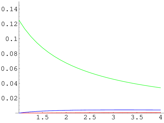
Figure 1: $c$ is on the horizontal-axis and the $\widetilde{{\cal U}}_{s}$ are on the vertical-axis. $\widetilde{{\cal U}}_{1}$ is represented by the red line, $\widetilde{{\cal U}}_{2}$ by the green line and $-\widetilde{{\cal U}}_{3,4}$ by the blue line

Figure 2: $c$ is on the horizontal-axis and $\sum_{s}\widetilde{{\cal U}}_{s}(c)$ is on the vertical-axis

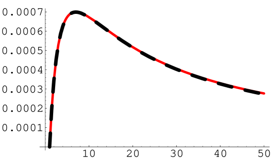
Figure 3: The red line is the sum ${\cal U}_{1}$ upto $J=100$ and the dashed black line upto $J=5$. $c$ is on the horizontal-axis.

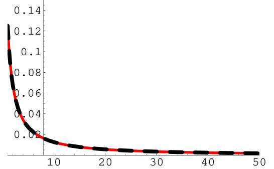
Figure 4: The red line is the sum ${\cal U}_{2}$ upto $J=100$ and the dashed black line upto $J=5$. $c$ is on the horizontal-axis.

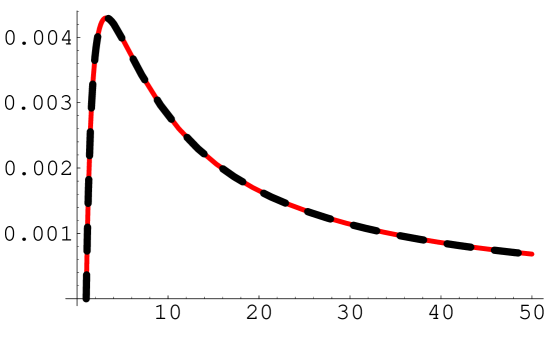
Figure 5: The red line is the sum ${\cal U}_{3,4}$ upto $J=100$ and the dashed black line upto $J=5$. $c$ is on the horizontal-axis.

References

- [1] R. C. Ferrell and D. M. Eardley, Phys. Rev. Lett. 59 (1987) 1617; R. C. Ferrell and D. M. Eardley, in “Frontiers in Numerical Relativity,” (eds. C. R. Evans, L. S. Finn, and D. W. Hobil, Cambridge U. Press, New York, 1989), pg. 27.
- [2] Kiyoshi Shiraishi, Nucl. Phys. B 402 (1993) 399–410.
- [3] R. Khuri and R. C. Myers, Nucl. Phys. B466 (1996) 60-74, hep-th/9512061.
- [4] David M. Kaplan and Jeremy Michelson, Phys. Lett. B410 (1997) 125-130, hep-th/9707021.
- [5] J. Michelson and A. Strominger, JHEP 9909 (1999) 005, hep-th/9908044; J. Michelson and A. Strominger, hep-th/9907191.
- [6] J. Gutowski and G. Papadopoulos, Phys. Lett. B432 (1998) 97-102, hep-th/9802186.
- [7] J. Gutowski and G. Papadopoulos, Phys. Lett. B472, 45 (2000) hep-th/9910022.
- [8] J. Gutowski and G. Papadopoulos, hep-th/0002242.
- [9] J. Maldacena, Adv. Theor. Math. Phys. 2, 231 (1998) hep-th/9711200.
- [10] O. Aharony, S.S. Gubser, J. Maldacena, H. Ooguri, and Y. Oz, Phys.Rept. 323 183-386 (2000) hep-th/9905111.
- [11] R. Britto-Pacumio, J. Michelson, A. Strominger, and A. Volovich, hep-th/9911066.
- [12] R. Britto-Pacumio, A. Strominger, and A. Volovich, hep-th/0004017.
- [13] A. Strominger and C. Vafa, Phys. Lett. B379 99-104 (1996), hep-th/9601029.
- [14] S. Surya and D. Marolf, Phys. Rev. D58 (1998) 124013, hep-th/9805121.
- [15] M. Douglas, J. Polchinski, and A. Strominger, JHEP 9712 (1997) 003, hep-th/9703031.
- [16] A.A. Tsyetlin, Nucl.Phys.Proc.Suppl. 68 (1998) 99-110, hep-th/9709123
- [17] J. Maldacena, Phys.Rev. D57 (1998) 3736-3741, hep-th/9705053
- [18] I. Chepelev and A.A. Tsyetlin, Nucl.Phys. B515 (1998) 73-113, hep-th/9709087
- [19] W. Israel and G. A. Wilson, J. Math. Phys. 13 (1972) 865.
- [20] G. W. Gibbons and P. J. Ruback, Phys. Rev. Lett. 57 (1986) 1492.
- [21] N. S. Manton, Phys. Lett. B110 54-56 (1982)
- [22] G. Gibbons, G. Papdopoulus, and K. S. Stelle, Nucl.Phys. B508 (1997) 623-658, hep-th/9706207.
- [23] G. Horowitz and A. Tsyetlin. Phys. Rev. D51 (1995) 2896-2917, hep-th/9409021.
- [24] J. Maharana and J. H. Schwartz. Nucl.Phys. B390 (1993) 3-32, hep-th/9207016.
- [25] J. Polchinski, String Theory Volume II, Cambridge University Press, 1998.
- [26] A. Peet and D. Marolf, hep-th 99–
- [27] Rose, Elementary theory of angular momentum, John Wiley, 1957.
- [28] Brink and Satchler, Angular momentum, Oxford: Clarendon Press, 1968