KUNS-1664 hep-th/0005123
Open membranes in a constant $C$-field background
and noncommutative boundary strings

We investigate the dynamics of open membrane boundaries in a constant $C$-field background. We follow the analysis for open strings in a $B$-field background, and take some approximations. We find that open membrane boundaries do show noncommutativity in this case by explicit calculations. Membrane boundaries are one dimensional strings, so we face a new type of noncommutativity, that is, noncommutative strings.

1 Introduction

It is surprising that, although it seems that noncommutative geometry is quite a pure mathematical object, noncommutativity does emerge in some definite limits of string theory. For instance, matrix theory compactified on tori gives Yang-Mills theory on noncommutative tori[1]; the quantization of open strings on a D-brane with a background $B$-field leads this D-brane world-volume to become noncommutative[2]; the twisted version of the reduced large-$N$ Super Yang-Mills model originally considered as a constructive definition of type IIB superstring can be interpreted as noncommutative Yang-Mills theory[3], and so on.

Recent development on string dualities reveals that M-theory rules nonperturbative features of superstring theories. It is natural to ask what is noncommutativity in M-theory. We do not know so much about M-theory. M-theory leads to eleven dimensional supergravity at the low-energy limit, and M-theory compactified on a circle becomes type IIA superstring by taking the limit for the radius of the circle to become zero. Moreover M-theory contains the two-dimensional extended object, M2-brane, as the fundamental component. Matrix theory proposed by Banks, Fischler, Shenker and Susskind [4] is considered as describing some (or complete as they state originally) degrees of freedom of M-theory. This matrix theory does show noncommutativity in some cases commented above. We can expect naturally that noncommutativity can emerge in M-theory.

On the other hand, a supersymmetric two-dimensional extended object, called supermembrane, is interesting in its connection to superstrings. A quantum extension of supermembrane is expected to give a definition of M-theory. Especially, it is well known that supermembrane in eleven dimensions can consistently couple to eleven dimensional supergravity as its backgrounds[5]. Thus, we have a natural question here; how does supermembrane theory show noncommutativity? It is a very meaningful question in two reasons. First, since we expect that supermembrane is a definition of M-theory, we also expect that supermembrane theory has noncommutativity in a definite limit or a background. Secondly, we wonder what is noncommutativity in more than two-dimensional extended objects. To clear this second point, let us compare it with the string case. In string theory, the end of open strings becomes noncommutative and a D-brane world-volume on which open strings can end has noncommutative geometry. Then, let us consider an open membrane which has one-dimensional boundary and focus on the behavior of these boundaries. Here, we face a conceptual jump. In string theory, open string ends are “points” and on a D-brane world-volume points do not commute with each other, while in membrane case, we find that its boundaries are “strings” and noncommutativity means one-dimensional strings do not commute with each other. Thus, we can learn a new feature of noncommutative geometry by studying membrane noncommutativity. A primitive analysis was carried out in [2].

In string theory, we can find noncommutativity by quantizing open strings in background NS-NS fields. Some authors have applied the Dirac procedure to boundary conditions[7, 8]. This method is very transparent and can be easily extended to other systems. We attempt to investigate an open membrane in a background three-form field in this way. It is well known that to investigate membrane theory has severe difficulties, for example, non-linearity of world-volume theory, non-renormalizability of three-dimensional sigma model, and so on. Thus, we must take an appropriate approximation, as explained later.

Our plan of investigation is as follows. In seeing the noncommutativity, supersymmetry was not essential in the string case. We drop the fermionic parts and consider a bosonic membrane. We start with a bosonic open membrane in a constant gauge field background. Since we should take our bosonic membrane as a toy model of eleven dimensional supermembrane, we restrict the background fields to the massless bosonic fields of eleven dimensional supergravity, the metric $g_{\mu\nu}$ and the three-form tensor field $C_{\mu\nu\rho}$. We consider only a bosonic background and drop the fermionic field, the gravitino $\chi^{\mu}$. Without introducing a two-form gauge field, there can not exist open membranes by gauge-invariance. Also in supermembrane case, we can not introduce an open supermembrane without braking all the supersymmetries in flat Minkowski space-time. However we can formulate a supersymmetric open supermembrane when there exists a “topological defect” as a background [6]. These defects are interpreted as, for instance, M5-brane, “end of the world” 9-plane in Hořava-Witten’s sense, etc. We shall introduce fixed $p$-branes in this bosonic case. We assume our open membranes are bounded to these “boundary planes,” and there is a two-form field, to which open membrane boundaries can couple, on these planes. In these settings, we calculate the Dirac brackets and confirm noncommutativity on these boundary planes. Our calculation is only to second order in $C$ and not exact.

This paper is organized as follows. In section 2, we propose our setup. We consider a bosonic open membrane in a constant $C$-field background. We suppose that one direction of the target space is compactified to a circle, another direction is compactified to an interval and there exist two fixed planes at the boundaries of this direction. We fix the reparametrization invariance of the world-volume with a static gauge and simplify the action by taking a limit. Equations of motion and boundary conditions are found, we go on to the canonical formalism and impose the boundary conditions as constraints. In section 3, we solve the constraints with an approximation. We take the radius of the compactification circle to be very large and the distance between the boundary planes to be infinitesimally small. In section 4, we calculate the Dirac brackets and confirm the noncommutativity on the boundary planes. Section 5 is served to discussions and remarks. In appendix A, we review the application of Dirac’s procedure for constrained systems to the boundary constraints in the string case.

2 An open membrane in a constant $C$-field

Let us consider an open membrane in the background of a constant three-form tensor field $C_{\mu\nu\rho}$. We suppose that our membrane topology is cylindrical and the background is eleven dimensional, compactified to $\textbf{R}^{9-p}\times M^{p}\times S^{1}\times I$, where $M^{p}$ is a $p$ dimensional flat Minkowski space-time and $I$ is an interval with a finite length. There exist at the boundaries of $I$ two $p$-branes on which an open membrane can end, and the $p$-branes wrap once around the $S^{1}$. $\textbf{R}^{9-p}\times I$ is transverse to these $p$-branes. We drop the fermionic part, that is, restrict ourselves to considering a bosonic membrane.

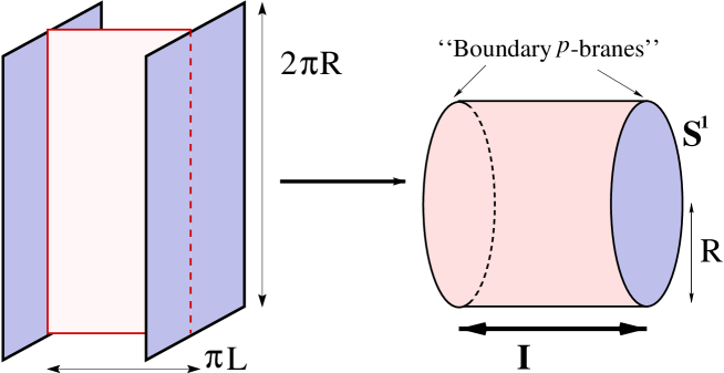
Figure 1: A membrane wrapped once around the compactification circle stretches between two fixed $p$-branes.

In this case, the action of the membrane is

$$S=-T\int\!\!d^{3}\xi\left\{\sqrt{-\det h_{\alpha\beta}}+\frac{1}{3!}\epsilon^{\alpha\beta\gamma}C_{\mu\nu\rho}\partial_{\alpha}X^{\mu}\partial_{\beta}X^{\nu}\partial_{\gamma}X^{\rho}\right\},$$ (1)

where $\xi^{\alpha}$ are the world-volume coordinates $(\tau,\sigma_{1},\sigma_{2})$ and $h_{\alpha\beta}$ is the induced metric on the world-volume, $h_{\alpha\beta}\equiv\partial_{\alpha}X^{\mu}\partial_{\beta}X_{\mu}$.

First, we fix the gauge freedom of world-volume reparametrization invariance with the static gauge,

$$\left\{\begin{array}[]{lcl}X^{0}=\tau&&\tau\in(-\infty,\infty)\\ X^{9}=\sigma_{1}L&&\sigma_{1}\in[0,\pi]\\ X^{10}=\sigma_{2}R&&\sigma_{2}\in[0,2\pi)\ ,\\ \end{array}\right.$$ (2)

and the radius of the compactified direction $X^{10}$ is $R$,

$$X^{10}\sim X^{10}+2\pi R.$$ (3)

We also compactify the $X^{9}$ direction on an interval. Suppose that there are two “fixed planes” placed at a distance of $\pi L$ in the $X^{9}$ direction. Here, $\pi L$ is the length of the interval, and the two boundaries of a membrane are bound to each of these “fixed planes”,

$$\Delta X^{9}=\pi L.$$ (4)

These “fixed planes” are, for example, regarded as M5-branes in M-theory when $p=5$. Since the dimension of the $p$-brane is not essential in our analysis, we assume $p=9$ from now on.

Under the static gauge condition,

$$\det h = \left|\begin{array}[]{ccc}-1+(\dot{X}^{i})^{2}&\dot{X}^{i}\partial_{1}X^{i}&\dot{X}^{i}\partial_{2}X^{i}\\ \dot{X}^{i}\partial_{1}X^{i}&L^{2}+(\partial_{1}X^{i})^{2}&\partial_{1}X^{i}\partial_{2}X^{i}\\ \dot{X}^{i}\partial_{2}X^{i}&\partial_{1}X^{i}\partial_{2}X^{i}&R^{2}+(\partial_{2}X^{i})^{2}\\ \end{array}\right|$$ (8)

$$= -L^{2}R^{2}+L^{2}R^{2}(\dot{X}^{i})^{2}-R^{2}(\partial_{1}X^{i})^{2}-L^{2}(\partial_{2}X^{i})^{2}+{\cal O}\left((\partial X)^{4}\right),$$ (9)

and we get the first part of the action (Dirac part) as

$$S_{\rm D}=T\int\!\!d^{3}\xi\left[-1+\frac{1}{2}(\dot{X}^{i})^{2}-\frac{1}{2}(\partial_{1}X^{i})^{2}-\frac{1}{2}(\partial_{2}X^{i})^{2}+{\cal O}\left((\partial X)^{4}\right)\right],$$ (10)

where we have made a rescaling, $L\sigma_{1}\rightarrow\sigma_{1}\ ,\ R\sigma_{2}\rightarrow\sigma_{2}$.

Next, we go on to consider the $C$-field part,

$$S_{C}=\int_{\Sigma}\!\!C_{[3]},$$ (11)

where $\Sigma$ is the world-volume of a membrane. At the beginning, note that our action (1) is not gauge-invariant for an open membrane. So as to make an open membrane gauge-invariant, we introduce a two-form gauge field $B$ coupled to the boundaries of a membrane,

$$S_{B}=\int_{\partial\Sigma}B_{[2]},$$ (12)

which transforms as $B\rightarrow B-\Lambda$ under the $C$-field gauge transformation, $C\rightarrow C+d\Lambda$, where $\Lambda$ is a two-form field. Here, this $B$-field is on the boundary planes and has the field strength $F\equiv dB$ on these planes. Gauge-invariance requires that $C$ and $F$ always appear with the form of $C+F$, so the constant $C$-field leads to a constant field strength $F$ on the boundary planes. Then, we gauge away $F$ and only consider the effects of the $C$-field. Moreover, we suppose that the $C$-field is not only constant but also “magnetic”, that is, their non-zero components are only $C_{ijk}$. Finally, the $C$-field part of the action is

$$S_{C}=-T\int\!\!d^{3}\xi\,C_{ijk}\dot{X}^{i}\partial_{1}X^{j}\partial_{2}X^{k},$$ (13)

where we have made a rescaling $C\rightarrow(LR)^{-1}C$.

A part of difficulties of membrane theory comes from its non-linearity of world-volume theory. Here, to avoid it, we take the limit $\alpha\rightarrow\infty$,

$$T \rightarrow\alpha^{2}T,$$

$$X \rightarrow\frac{1}{\alpha}X,$$

$$C \rightarrow\alpha C,$$

and also drop the constant term of the Dirac part. This limit means that the self-interactions of the world-volume theory are weak compared to the interactions with the background gauge fields. Finally, we get the effective action as follows,

$$S^{\rm eff}=T\int\!\!d^{3}\xi\left[\frac{1}{2}\left\{(\dot{X}^{i})^{2}-(\partial_{1}X^{i})^{2}-(\partial_{2}X^{i})^{2}\right\}-C_{ijk}\dot{X}^{i}\partial_{1}X^{j}\partial_{2}X^{k}\right]\ ,$$ (14)

where the ranges of the world-volume coordinates are

$$\sigma_{1} \in[0,\pi L],$$ (15)

$$\sigma_{2} \in[0,2\pi R),$$ (16)

and the area of the membrane is $2\pi^{2}LR$.

To find the equations of motion and the boundary conditions, we vary the effective action (14),

$$\delta S^{\rm eff} =-T\int\!\!d^{3}\xi\left[\ddot{X}^{i}-(\partial_{1})^{2}X^{i}-(\partial_{2})^{2}X^{i}\right]\delta X^{i}$$

$$\phantom{aa}+T\int\!\!d^{3}\xi\partial_{1}\left[\left(-\partial_{1}X^{i}-C_{ijk}\dot{X}^{k}\partial_{2}X^{j}\right)\delta X^{i}\right]\ .$$ (17)

$\delta S^{\rm eff}=0$ leads to the equations of motion,

$$\square X^{i}=0,$$ (18)

where $\square\equiv\eta^{\alpha\beta}\partial_{\alpha}\partial_{\beta}=\partial_{\tau}^{2}-\partial_{1}^{2}-\partial_{2}^{2}$, and also leads to the boundary conditions,

$$\left.\partial_{1}X^{i}-C_{ijk}\dot{X}^{j}\partial_{2}X^{k}\right|_{\sigma_{1}=0,\pi L}=0.$$ (19)

The conjugate momenta are

$$P_{i}=\frac{\delta}{\delta\dot{X}^{i}}L=T\left(\dot{X}_{i}-C_{ijk}\partial_{1}X^{j}\partial_{2}X^{k}\right)\ ,$$ (20)

so the Hamiltonian is

$$H \equiv\int\!\!d^{2}\sigma\left(\dot{X}^{i}P_{i}-{\cal L}\right)$$

$$=\frac{T}{2}\int\!\!d^{2}\sigma\left[\left(\frac{P^{i}}{T}+C_{ijk}\partial_{1}X^{j}\partial_{2}X^{k}\right)^{2}+(\partial_{1}X^{i})^{2}+(\partial_{2}X^{i})^{2}\right].$$ (21)

To follow the calculations in the string case[7, 8], we regard the boundary conditions as primary constraints,

$$\phi^{i}_{1}=\left.\partial_{1}X^{i}-C_{ijk}\left(\frac{P^{j}}{T}+C_{jlm}\partial_{1}X^{l}\partial_{2}X^{m}\right)\partial_{2}X^{k}\right|_{\sigma_{1}=0,\pi L}\approx 0\ .$$ (22)

Poisson brackets are ordinarily defined as

$$\begin{array}[]{l}\left\{X^{i}(\sigma_{1},\sigma_{2}),P_{j}(\sigma^{\prime}_{1},\sigma^{\prime}_{2})\right\}=\delta^{i}_{j}\delta^{2}(\sigma-\sigma^{\prime}),\\ \left\{X^{i},X^{j}\right\}=\left\{P_{i},P_{j}\right\}=0.\end{array}$$ (23)

Using these, we get the equations of motion,

$$\dot{X}^{i}\equiv\left\{X^{i}(\sigma),H\right\}=\frac{P^{i}}{T}+C_{ijk}\partial_{1}X^{j}\partial_{2}X^{k},$$ (24)

and

$$\dot{P}^{i}\equiv\left\{P_{i}(\sigma),H\right\} =T\left\{\ddot{X}^{i}-C_{ijk}\left(\partial_{1}\dot{X}^{j}\partial_{2}X^{k}+\partial_{1}X^{j}\partial_{2}\dot{X}^{k}\right)\right\}$$

$$=T\left[C_{ijk}\left(\partial_{2}X^{j}\partial_{1}\left(\frac{P^{k}}{T}+C_{klm}\partial_{1}X^{l}\partial_{2}X^{m}\right)\right.\right.$$

$$\phantom{aaaa}\left.\left.-\partial_{1}X^{j}\partial_{2}\left(\frac{P^{k}}{T}+C_{klm}\partial_{1}X^{l}\partial_{2}X^{m}\right)\right)+\Delta X^{i}\right],$$ (25)

where Laplacian $\Delta$ is defined as $\partial_{1}^{2}+\partial_{2}^{2}$ and dot means $\tau$ derivative.

For simplicity, we set $T=1$. We can recover $T$ by replacing $P$ with $P/T$.

3 Solving constraints

The method described in appendix A leads us to find the Dirac brackets of the membrane in the constant $C$-field. First, we consider the consistency conditions of the constraints

$$\dot{\phi}\equiv\left\{\phi,H_{\rm T}\right\}\approx 0\ ,$$ (26)

and find an infinite chain of secondary constraints as follows

$$\phi_{2}^{i} \equiv\dot{\phi}_{1}^{i}=\left\{\phi_{1}^{i},H\right\}$$

$$=\partial_{1}\dot{X}^{i}-C_{ijk}\ddot{X}^{j}\partial_{2}X^{k}-C_{ijk}\dot{X}^{j}\partial_{2}\dot{X}^{k}\ ,$$

$$\phi_{3}^{i} \equiv\dot{\phi}_{2}^{i}$$

$$=\partial_{1}\ddot{X}^{i}-C_{ijk}\left[X^{{(3)}j}\partial_{2}X^{k}+2\ddot{X}^{j}\partial_{2}\dot{X}^{k}+\dot{X}^{j}\partial_{2}\ddot{X}^{k}\right]\ ,$$

$$\vdots$$

$$\phi_{n+1}^{i} \equiv\phi^{{(n)}i}_{1}$$

$$=\partial_{1}X^{{(n)}i}_{1}-C_{ijk}\sum^{\infty}_{\ell=0}\begin{pmatrix}n\cr\ell\cr\end{pmatrix}X^{{(n+1-\ell)\/}j}\partial_{2}X^{{(\ell)\/}k}\ ,$$ (27)

where

$$\phi^{{(n)}i}\equiv\frac{\partial^{n}}{\partial\tau^{n}}\phi^{i}\ .$$ (28)

Note that the equation of motion (24) tells that each secondary constraint has at most $C^{3}$, and all the constraints are second class. Explicit computations show that the first few constraints are given by

$$\phi^{i}_{1} =\left.\partial_{1}X^{i}-C_{ijk}\left(P^{j}+C_{jlm}\partial_{1}X^{j}\partial_{2}X^{k}\right)\partial_{2}X^{k}\right|_{\sigma_{1}=0,\pi L}\approx 0,$$ (29)

$$\phi^{i}_{2} =\partial_{1}P^{i}$$

$$+C_{ijk}\left[\partial_{1}X^{j}\partial_{1}\partial_{2}X^{k}-\partial_{2}^{2}X^{j}\partial_{2}X^{k}-P^{j}\partial_{2}P^{k}\right]$$

$$+C_{ijk}C_{jlm}\left[-\partial_{2}P^{k}\partial_{1}X^{l}\partial_{2}X^{m}+P^{k}\partial_{2}(\partial_{1}X^{l}\partial_{2}X^{m})\right]$$

$$\left.-C_{ijk}C_{jlm}C_{kop}[\partial_{1}X^{l}\partial_{2}X^{m}\partial_{2}(\partial_{1}X^{o}\partial_{2}X^{p})]\right|_{\sigma_{1}=0,\pi L}\approx 0,$$ (30)

$$\phi^{i}_{3} =\partial_{1}\Delta X^{k}$$

$$+C_{ijk}[-\Delta P^{j}\partial_{2}X^{k}+2\partial_{2}P^{j}\Delta X^{k}-P^{j}\partial_{2}\Delta X^{k}]$$

$$+C_{ijk}C_{jlm}\left[2\Delta X^{k}\partial_{2}(\partial_{1}X^{l}\partial_{2}X^{m})\right.$$

$$\left.\phantom{+C_{ijk}C_{jlm}[2\Delta]}\left.-\partial_{2}X^{k}\Delta(\partial_{1}X^{l}\partial_{2}X^{m})-\partial_{2}\Delta X^{k}(\partial_{1}X^{l}\partial_{2}X^{m})\right]\right|_{\sigma_{1}=0,\pi L}\approx 0.$$ (31)

These constraints look too hard to solve completely unlike the string case. Thus, we shall take an approximation to solve them.

At this stage, we take the limit $L\rightarrow 0$ and $R\rightarrow\infty$ . This leads to simplification as follows. For $\sigma_{1}$, we suppose that no oscillations are excited. Hence, after solving the constraints, $X^{i}(\tau,\sigma_{1},\sigma_{2})$ and $P^{i}(\tau,\sigma_{1},\sigma_{2})$ are determined by their boundary values. And for $\sigma_{2}$, we neglect terms which is of order $(1/R)^{3}$ or higher, which means that we drop the terms involving three derivatives of $\sigma_{2}$ or higher,

$$\partial_{2}^{3}X^{i}=0\ ,\ \partial_{2}^{2}X^{i}\partial_{2}X^{j}=0\quad\text{etc$\ldots$}\ .$$ (32)

To solve the constraints, we shall include the effects of the $C$-field order by order. At order of $C^{0}$, the boundary conditions are

$$\left.\partial_{1}X^{i}\right|_{\sigma_{1}=0,\pi L}=0\quad\text{and}\quad X^{i}(\tau,\sigma_{1},\sigma_{2})=X^{i}(\tau,\sigma_{1},\sigma_{2}+2\pi R).$$ (33)

Since no oscillations of $\sigma_{1}$ are excited under the $L\rightarrow 0$ limit, the solution is

$$X^{i}(\tau,\sigma_{1},\sigma_{2})=x^{(0)i}_{0}(\tau,\sigma_{2}).$$ (34)

where the subscript $0$ of $x^{(0)i}_{0}$ means we are considering only the zero-mode of $\sigma_{1}$. Since the $C$-field background changes the $\sigma_{1}$ boundary conditions, the $\sigma_{1}$ dependence of fields $X$ and $P$ would be altered:

$$X^{i}=x^{(0)i}_{0}(\tau,\sigma_{2})+(\text{corrections which depend also on $\sigma_{1}$ and $C$}).$$ (35)

Let us calculate the corrections to second order in $C$. Consider the expansions of $X$ and $P$ in terms of $C$

$$X^{i}_{0}(\tau,\sigma_{1},\sigma_{2})=x_{0}^{(0)i}+x_{0}^{(1)i}+x_{0}^{(2)i},$$ (36)

$$P^{i}_{0}(\tau,\sigma_{1},\sigma_{2})=p_{0}^{(0)i}+p_{0}^{(1)i}+p_{0}^{(2)i},$$ (37)

where $x_{0}^{(0)}$ and $p_{0}^{(0)}$ are functions of $\tau$ and $\sigma_{2}$, independent of $\sigma_{1}$ and unconstrained. We substitute them into the constraints (29) and (3). Of order $C^{1}$, we get

$$\phi_{1}^{i} =\left.\partial_{1}x_{0}^{(1)i}-C_{ijk}p_{0}^{(0)j}\partial_{2}x_{0}^{(0)k}\right|_{\sigma_{1}=0,\pi L}\approx 0,$$

$$\phi_{2}^{i} =\left.\partial_{1}p_{0}^{(1)i}+C_{ijk}\left(-p_{0}^{(0)j}\partial_{2}p_{0}^{(0)k}\right)\right|_{\sigma_{1}=0,\pi L}\approx 0,$$ (38)

and find solutions at this order as follows

$$x_{0}^{(1)i}(\tau,\sigma_{1},\sigma_{2})=A_{0}^{(1)i}(\tau,\sigma_{2})+C_{ijk}p_{0}^{(0)j}\partial_{2}x_{0}^{(0)k}\cdot\sigma_{1},$$ (39)

$$p_{0}^{(1)i}(\tau,\sigma_{1},\sigma_{2})=B_{0}^{(1)i}(\tau,\sigma_{2})+C_{ijk}p_{0}^{(0)j}\partial_{2}p_{0}^{(0)k}\cdot\sigma_{1},$$ (40)

where $A_{0}$ and $B_{0}$ in the right hand sides are unconstrained. In succession, the equations of order $C^{2}$ are

$$\phi_{1}^{i} =\partial_{1}x_{0}^{(2)i}-C_{ijk}\left[p_{0}^{(1)j}\partial_{2}x_{0}^{(0)k}+p_{0}^{(0)j}\partial_{2}x_{0}^{(1)k}\right]$$

$$\phantom{aaa}-C_{ijk}C_{jlm}\left(p_{0}^{(0)l}\partial_{2}p_{0}^{(0)m}\partial_{2}x_{0}^{(0)k}-p_{0}^{(0)l}\partial_{2}x_{0}^{(0)m}p_{0}^{(0)k}\right)\cdot\sigma_{1},$$ (41)

$$\phi_{2}^{i} =\partial_{1}p_{0}^{(2)i}-C_{ijk}\left[p_{0}^{(1)j}\partial_{2}p_{0}^{(0)k}+p_{0}^{(0)j}\partial_{2}p_{0}^{(1)k}\right]$$

$$\phantom{aaa}-C_{ijk}C_{jlm}\left(p_{0}^{(0)l}\partial_{2}p_{0}^{(0)m}\partial_{2}p_{0}^{(0)k}-p_{0}^{(0)l}\partial_{2}p_{0}^{(0)m}p_{0}^{(0)k}\right)\cdot\sigma_{1},$$ (42)

and we find the solutions,

$$x_{0}^{(2)i}(\tau,\sigma_{1},\sigma_{2}) =A_{0}^{(2)i}(\tau,\sigma_{2})+C_{ijk}\left[B_{0}^{(1)j}\partial_{2}x_{0}^{(0)k}+p_{0}^{(0)j}\partial_{2}A_{0}^{(1)k}\right]\sigma_{1}$$

$$\phantom{aaa}+C_{ijk}C_{jlm}\left(p_{0}^{(0)l}\partial_{2}p_{0}^{(0)m}\partial_{2}x_{0}^{(0)k}-p_{0}^{(0)l}\partial_{2}x_{0}^{(0)m}p_{0}^{(0)k}\right)\cdot\frac{\sigma_{1}^{2}}{2},$$

$$p_{0}^{(2)i}(\tau,\sigma_{1},\sigma_{2}) =B_{0}^{(2)i}(\tau,\sigma_{2})+C_{ijk}\left[B_{0}^{(1)j}\partial_{2}p_{0}^{(0)k}+p_{0}^{(0)j}\partial_{2}B_{0}^{(1)k}\right]\sigma_{1}$$

$$\phantom{aaa}+C_{ijk}C_{jlm}\left(p_{0}^{(0)l}\partial_{2}p_{0}^{(0)m}\partial_{2}p_{0}^{(0)k}-p_{0}^{(0)l}\partial_{2}p_{0}^{(0)m}p_{0}^{(0)k}\right)\cdot\frac{\sigma_{1}^{2}}{2}\ .$$ (43)

Putting them together, we find that the $X^{i}(\tau,\sigma_{1},\sigma_{2})$ and $P^{i}(\tau,\sigma_{1},\sigma_{2})$ are determined by the unconstrained boundary values, $X_{0}(\tau,\sigma_{2})=x_{0}^{(0)}+A_{0}^{(1)}+A_{0}^{(2)}$ and $P_{0}(\tau,\sigma_{2})=p_{0}^{(0)}+B_{0}^{(1)}+B_{0}^{(2)}$ as follows,

$$X^{i}(\tau,\sigma_{1},\sigma_{2})= X^{i}_{0}+\sigma_{1}C_{ijk}P_{0}^{j}\partial_{2}X_{0}^{k}$$

$$+\frac{\sigma_{1}^{2}}{2}C_{ijk}C_{jlm}\left[\partial_{2}X_{0}^{k}P_{0}^{l}\partial_{2}P_{0}^{m}-P_{0}^{k}\partial_{2}(P_{0}^{l}\partial_{2}X_{0}^{m})\right],$$ (44)

$$P^{i}(\tau,\sigma_{1},\sigma_{2})= P_{0}^{i}+\sigma_{1}C_{ijk}P_{0}^{j}\partial_{2}P_{0}^{k}$$

$$+\frac{\sigma_{1}^{2}}{2}C_{ijk}C_{jlm}\left[\partial_{2}P_{0}^{k}P_{0}^{l}\partial_{2}P_{0}^{m}-P_{0}^{k}\partial_{2}(P_{0}^{l}\partial_{2}P_{0}^{m})\right].$$ (45)

One can confirm that these solutions satisfy the remaining constraints by substituting (3) and (3) into the explicit form of $\phi_{3}^{i}$ and taking into account the fact that the other higher constraints involve only higher derivative terms of $\sigma_{1}$ and $\sigma_{2}$. Since we get the solutions of the constraints, we can compute the Dirac brackets of $X$ and $P$ by the method given in appendix A. This is what we shall do in the following section.

4 Computing the Dirac brackets

In order to compute the Dirac brackets, we first calculate Lagrange brackets. In this case, Lagrange bracket L is defined as

$$\Omega= -2\int\!\!d^{2}\sigma dX^{i}(\sigma_{1},\sigma_{2})\wedge dP^{i}(\sigma_{1},\sigma_{2})$$

$$= \int\!\!dxdy\,{\bf L}^{ij}_{xy}\,d\phi^{i}(x)\wedge d\phi^{j}(y),$$ (46)

where we have integrated over $\sigma_{1}$, $d\phi=dX_{0}(\sigma_{2})$ or $dP_{0}(\sigma_{2})$, and $x$ and $y$ denote the $\sigma_{2}$ coordinate. Dirac bracket C is determined by the inverse matrix of this Lagrange brackets, $\textbf{C}=\textbf{L}^{-1}$. To calculate the Lagrange bracket of this system, we determine the effects of the $C$-field order by order, to order $C^{2}$:

$${\bf L}={\bf L}^{(0)}+{\bf L}^{(1)}+{\bf L}^{(2)},$$ (47)

where $L^{(i)}$ denotes the terms of order $C^{i}$. Then the Dirac bracket is obtained as

$${\bf C}=\textbf{L}^{-1}= {\bf L}^{(0){-1}}-{\bf L}^{(0){-1}}({\bf L}^{(1)}+{\bf L}^{(2)}){\bf L}^{(0){-1}}+{\bf L}^{(0){-1}}{\bf L}^{(1)}{\bf L}^{(0){-1}}{\bf L}^{(1)}{\bf L}^{(0){-1}}+{\cal O}(C^{3})$$ (48)

$$= {\bf J}-{\bf J}({\bf L}^{(1)}+{\bf L}^{(2)}){\bf J}+{\bf J}{\bf L}^{(1)}{\bf J}{\bf L}^{(1)}{\bf J}+{\cal O}(C^{3}),$$ (49)

where we have abbreviated ${\bf L}^{(0){-1}}$ as ${\bf J}$.

Let us start the calculation. In zeroth order in $C$, the Lagrange bracket is determined through the symplectic form

$$\Omega^{[0]}= -2\int\!\!d\sigma^{2}dX_{0}^{i}\wedge dP_{0}^{i}$$

$$= -2\pi L\int\!\!dxdy\,\delta^{ij}\,\delta(x-y)\,dX_{0}^{i}(x)\wedge dP_{0}^{j}(y)\ .$$ (50)

We get

$${\bf L}^{(0)}=\left(\begin{array}[]{cc}0&L^{(0)}\\ -(L^{(0)})^{\rm T}&0\\ \end{array}\right),$$ (51)

where

$$L^{(0)}=-\pi L\delta^{ij}\delta(x-y).$$ (52)

The inverse matrix of this ${\bf L}^{(0)}$ is given by

$${\bf J}=({\bf L}^{(0)})^{-1}=\left(\begin{array}[]{cc}&-J\\ J&\\ \end{array}\right)\ ,\ J=(L^{(0)})^{-1}=-\frac{1}{\pi L}\,\delta^{ij}\,\delta(x-y)\ ,\ J^{\rm T}=J\ .$$ (53)

At this stage, we can calculate the Dirac bracket at $C=0$:

$$\left\{X_{0}^{i}(x),X_{0}^{j}(y)\right\}_{\rm DB}= 0,$$ (54)

$$\left\{P_{0}^{i}(x),P_{0}^{j}(y)\right\}_{\rm DB}= 0,$$ (55)

$$\left\{X_{0}^{i}(x),P_{0}^{j}(y)\right\}_{\rm DB}= \frac{1}{\pi L}\,\delta^{ij}\,\delta(x-y)\ .$$ (56)

These are the original Poisson brackets except for the normalization factor.

Calculations of ${\cal O}(C^{1})$

Next, we shall calculate the $C^{1}$ part. This is the first non-trivial result in these calculations. The symplectic form of this order is

$$\Omega^{[1]}= -2\int\!\!\,d^{2}\sigma\ \left[\sigma_{1}\,C_{ikl}\,dX_{0}^{i}\wedge(dP_{0}^{k}\partial_{2}P_{0}^{l}+P_{0}^{k}\partial_{2}dP_{0}^{l})\right.$$

$$\phantom{-2\int\!\!d^{2}\sigma\sigma_{1}C_{ikl}}\left.+\sigma_{1}C_{ikl}(dP_{0}^{k}\partial_{2}X_{0}^{l}+P_{0}^{k}\partial_{2}dX_{0}^{l})\wedge dP_{0}^{i}\right]$$

$$= -(\pi L)^{2}\int\!\!dxdy\,C_{ijl}\,\left[dX_{0}^{i}(x)\wedge dP_{0}^{j}(y)\left(-2C_{ijl}P_{0}^{l}(x)\partial_{x}\delta(x-y)\right)\right.$$

$$\phantom{aaaaaaaaaaaaaaaaa}\left.-dP_{0}^{i}(x)\wedge dP_{0}^{j}(y)\partial_{x}X_{0}^{l}\,\delta(x-y)\right],$$ (57)

and we get

$${\bf L}^{(1)}=\left(\begin{array}[]{cc}0&L^{(1)}\\ -(L^{(1)})^{\rm T}&l^{(1)}\\ \end{array}\right),$$ (58)

where

$$L^{(1)}= (\pi L)^{2}C_{ijl}P_{0}^{l}(x)\partial_{x}\delta(x-y),$$ (59)

$$l^{(1)}= (\pi L)^{2}C_{ijl}\partial_{x}X_{0}^{l}\delta(x-y)\ .$$ (60)

At this order, the Dirac bracket is

$$\left\{X_{0}^{i}(x),X_{0}^{j}(y)\right\}_{\rm DB}= C_{ijl}\partial_{x}X_{0}^{l}\,\delta(x-y),$$ (61)

$$\left\{P_{0}^{i}(x),P_{0}^{j}(y)\right\}_{\rm DB}= 0,$$ (62)

$$\left\{X_{0}^{i}(x),P_{0}^{j}(y)\right\}_{\rm DB}= \frac{1}{\pi L}\,\delta^{ij}\,\delta(x-y)-C_{ijl}P_{0}^{l}(y)\delta^{\prime}(y-x)\ .$$ (63)

One can check that the Jacobi identity holds at this order,

$$\left\{\left\{X_{0}^{i}(x),P_{0}^{j}(y)\right\},X_{0}^{k}(z)\right\}+\mbox{\rm(cyclic.) }$$

$$=\frac{1}{\pi L}C_{ijk}\left(\delta(y-z)\delta^{\prime}(y-x)+\delta(y-x)\delta^{\prime}(y-z)+\delta(z-x)\delta^{\prime}(z-y)\right)$$

$$=\frac{1}{\pi L}C_{ijk}\left(\delta(y-z)\delta^{\prime}(y-x)+\delta(y-x)\delta^{\prime}(y-z)+\delta(y-x)\delta^{\prime}(z-y)-\delta^{\prime}(z-x)\delta(z-y)\right)$$

$$=0\ .$$ (64)

The Jacobi identity for $\left\{X,\left\{X,X\right\}\right\}$ is trivially satisfied at first order in $C$. To see how it is non-trivially satisfied, we turn to the calculations of $C^{2}$.

Calculations of ${\cal O}(C^{2})$

The calculations of order $C^{2}$ turn out to be very complicated, so we split the calculations into some parts.

First, we consider the cross terms, $(C^{1}\text{ part})\wedge(C^{1}\text{ part})$ . The symplectic form of this part is

$$\Omega^{[2-1]}= -2\int\!\!d^{2}\sigma\,\sigma_{1}^{2}\ C_{ijk}C_{ilm}\,(dP_{0}^{j}\partial_{2}X_{0}^{k}+P_{0}^{j}\partial_{2}dX_{0}^{k})\wedge(dP_{0}^{l}\partial_{2}P_{0}^{m}+P_{0}^{l}\partial_{2}dP_{0}^{m})$$

$$= -\frac{2(\pi L)^{3}}{3}\int\!\!d^{2}\sigma\,C_{ikl}C_{jml}$$

$$\times\left\{dX_{0}^{i}(x)\wedge dP_{0}^{j}(y)\partial_{x}\left(P_{0}^{k}(x)\left(2\partial_{y}P_{0}^{m}(y)+P_{0}^{m}(y)\partial_{y}\right)\delta(x-y)\right)\phantom{\frac{}{}}\right.$$

$$\phantom{aaaaaa}+dP_{0}^{i}(x)\wedge dP_{0}^{j}(y)\left[\frac{1}{2}\left(X_{0}^{k\prime}(x)P_{0}^{m\prime}(x)-P_{0}^{k\prime}(y)X_{0}^{m\prime}(y)\right)\delta(x-y)\right.$$

$$\left.\left.\phantom{\frac{}{}AAAAAAAAAAAAAA}-\left(X_{0}^{k\prime}(x)P_{0}^{m}(x)+P_{0}^{k}(y)X_{0}^{m\prime}(y)\right)\delta^{\prime}(x-y)\right]\right\}\ ,$$ (65)

so we get

$${\bf L}^{[2-1]}=\left(\begin{array}[]{cc}&L^{[2-1]}\\ -(L^{[2-1]})^{\rm T}&l^{[2-1]}\\ \end{array}\right)\ ,$$ (66)

where

$$L^{[2-1]} =-\frac{(\pi L)^{3}}{3}C_{ikl}C_{jml}\partial_{x}\left(P_{0}^{k}(x)\left(2\partial_{y}P_{0}^{m}(y)+P_{0}^{m}(y)\partial_{y}\right)\delta(x-y)\right),$$ (67)

$$l^{[2-1]} =-\frac{1}{3}(\pi L)^{3}C_{ikl}C_{jml}\left(\left(X_{0}^{k\prime}(x)P_{0}^{m\prime}(x)-P_{0}^{k\prime}(y)X_{0}^{m\prime}(y)\right)\delta(x-y)\right.$$

$$\phantom{AAAAAAA}-\left.\left(X_{0}^{k\prime}(x)P_{0}^{m}(x)+P_{0}^{k}(y)X_{0}^{m\prime}(y)\right)\delta^{\prime}(x-y)\right)\ .$$ (68)

Next, we consider the $(C^{0}\text{ part})\wedge(C^{2}\text{ part})$. The symplectic form of this part is

$$\Omega^{[2-2]} =-2\int\!\!d^{2}\sigma\,\sigma_{1}^{2}\ C_{ijk}C_{ilm}$$

$$\phantom{aaaa}\times\left\{\left[\partial_{2}dX_{0}^{k}P_{0}^{l}\partial_{2}P_{0}^{m}+\partial_{2}X_{0}^{k}dP_{0}^{l}\partial_{2}P_{0}^{m}-\partial_{2}X_{0}^{k}P_{0}^{m}\partial_{2}dP_{0}^{l}\right.\right.$$

$$\phantom{aaaaaaaaaaaaa}\left.-dP_{0}^{k}\partial_{2}(P_{0}^{l}\partial_{2}X_{0}^{m})-P_{0}^{k}\partial_{2}(dP_{0}^{l}\partial_{2}X_{0}^{m}-P_{0}^{m}\partial_{2}dX_{0}^{l})\right]\wedge dP_{0}^{i}$$

$$\phantom{aaaaaaa}+dX_{0}^{i}\wedge\left[\partial_{2}dP_{0}^{k}P_{0}^{l}\partial_{2}P_{0}^{m}-\partial_{2}P_{0}^{k}P_{0}^{m}\partial_{2}dP_{0}^{l}+\partial_{2}P_{0}^{k}dP_{0}^{l}\partial_{2}P_{0}^{m}\right.$$

$$\left.\left.\phantom{aaaaaaaaaaaaaa}-dP_{0}^{k}\partial_{2}(P_{0}^{l}\partial_{2}P_{0}^{m})-P_{0}^{k}\partial_{2}(dP_{0}^{l}\partial_{2}P_{0}^{m}-P_{0}^{m}\partial_{2}dP_{0}^{l})\right]\right\}.$$ (69)

Then we find that the $\Omega^{[2-2]}$ has the form

$$\Omega^{[2-2]}=\int\!\!dxdy{\bf L}^{[2-2]}d\phi^{i}(x)\wedge d\phi^{j}(y)\ ,$$ (70)

where

$${\bf L}^{[2-2]}={\bf M}+{\bf N},$$ (71)

$$({\bf M})^{ij}_{xy}=\left(\begin{array}[]{cc}&M\\ -M^{\rm T}&m\\ \end{array}\right)\ ,$$ (72)

$$({\bf N})^{ij}_{xy}=\left(\begin{array}[]{cc}&N\\ -N^{\rm T}&n\\ \end{array}\right)\ ,$$ (73)

and, ${\bf M}$ and ${\bf N}$ correspond to the following tensor structures of $C^{2}$:

$${\bf M} \propto C_{ijk}C_{klm},$$

$${\bf N} \propto C_{ikl}C_{jml}\ .$$

The explicit calculations of M and N are shown in appendix B. The results are

$$M =\frac{(\pi L)^{3}}{3}C_{ijk}C_{klm}\left[P_{0}^{l}(x)\partial_{x}P_{0}^{m}(x)\delta^{\prime}(x-y)\right],$$ (74)

$$m =\frac{(\pi L)^{3}}{3}C_{ijk}C_{klm}\partial_{y}\left(P_{0}^{l}(y)\partial_{y}X_{0}^{m}(y)\right)\delta(x-y),$$ (75)

$$N =\frac{(\pi L)^{3}}{3}C_{ikl}C_{jml}\left[P_{0}^{k}(x)P_{0}^{m}(x)\delta^{\prime\prime}(x-y)+P_{0}^{m\prime}(x)\partial_{x}\left(P_{0}^{k}(x)\delta(x-y)\right)\right],$$ (76)

$$n =\frac{(\pi L)^{3}}{3}C_{ikl}C_{jml}\left[X_{0}^{k\prime}(x)P_{0}^{m}(x)+X_{0}^{m\prime}(y)P_{0}^{k}(y)\right]\delta^{\prime}(x-y).$$ (77)

Thus we get the Lagrange brackets to order $C^{2}$. Let us compute the Dirac brackets.

Computing the Dirac brackets

By (48), we can calculate the Dirac brackets C,

$$\textbf{C}^{ij}_{xy}=\begin{pmatrix}\left\{X_{0}^{i}(x),X_{0}^{j}(y)\right\}_{\rm DB}&\left\{X_{0}^{i}(x),P_{0}^{j}(y)\right\}_{\rm DB}\cr-\left\{P_{0}^{j}(y),X_{0}^{i}(x)\right\}_{\rm DB}&\left\{P_{0}^{i}(x),P_{0}^{j}(y)\right\}_{\rm DB}\cr\end{pmatrix},$$ (78)

as follows:

$$\left\{X_{0}^{i}(x),X_{0}^{j}(y)\right\}_{\rm DB} =J\left(l^{(1)}\right)J+J\left(l^{(2)}\right)J-Jl^{\small(1)}JL^{\small(1)}J-J(L^{\small(1)})^{\rm T}Jl^{\small(1)}J$$

$$=\frac{1}{(\pi L)^{2}}\left(l^{(1)}\right)^{ij}_{xy}+\frac{1}{(\pi L)^{2}}\left(l^{(2)}\right)^{ij}_{xy}$$

$$\phantom{aaa}+\frac{1}{(\pi L)^{3}}\left\{(l^{\small(1)})^{il}_{xz}(L^{\small(1)})^{lj}_{zy}+\left((L^{\small(1)})^{\rm T}\right)^{il}_{xz}(l^{\small(1)})^{lj}_{zy}\right\}+{\cal O}(C^{3}),$$ (79)

$$\left\{X_{0}^{i}(x),P_{0}^{j}(y)\right\}_{\rm DB} =-J+J\left((L^{(1)})^{\rm T}\right)J+J\left((L^{(2)})^{\rm T}\right)J-J(L^{\small(1)})^{\rm T}J(L^{\small(1)})^{\rm T}J$$

$$=\frac{1}{\pi L}({\bf 1})^{ij}_{xy}+\frac{1}{(\pi L)^{2}}\left((L^{(1)})^{\rm T}\right)^{ij}_{xy}$$

$$\phantom{aaa}+\frac{1}{(\pi L)^{2}}\left((L^{(2)})^{\rm T}\right)^{ij}_{xy}+\frac{1}{(\pi L)^{3}}\left((L^{\small(1)})^{\rm T}\right)^{il}_{xz}\left((L^{\small(1)})^{\rm T}\right)^{lj}_{zy}+{\cal O}(C^{3}),$$ (80)

$$\left\{P_{0}^{i}(x),P_{0}^{j}(y)\right\}_{\rm DB} =0\ .$$ (81)

Explicit computation shows

$$\left\{X_{0}^{i}(x),X_{0}^{j}(y)\right\}_{\rm DB} =C_{ijl}X_{0}^{l\prime}(x)\delta(x-y)$$

$$\phantom{aa}-\frac{1}{3}C_{ikl}C_{jml}\left[\left(X_{0}^{k\prime}(x)P_{0}^{m\prime}(x)-X_{0}^{m\prime}(y)P_{0}^{k\prime}(y)\right)\delta(x-y)\right.$$

$$\left.\phantom{aaAAAAAAAAA}+\left(X_{0}^{k\prime}(x)P_{0}^{m}(x)+X_{0}^{m\prime}(y)P_{0}^{k}(y)\right)\delta^{\prime}(x-y)\right]$$

$$\phantom{aaaa}+\frac{1}{3}C_{ijk}C_{klm}\partial_{y}\left(P_{0}^{l}(y)X_{0}^{m\prime}(y)\right)\delta(x-y)\ +{\cal O}(C^{3}),$$ (82)

$$\left\{X_{0}^{i}(x),P_{0}^{j}(y)\right\}_{\rm DB} =\delta^{ij}\delta(x-y)+C_{ijl}P_{0}^{l}(y)\delta^{\prime}(x-y)$$

$$\phantom{aa}-\frac{1}{3}C_{ikl}C_{jml}\left[P_{0}^{k}(x)P_{0}^{m}(x)\delta^{\prime\prime}(x-y)\right.+3P_{0}^{k}(x)P_{0}^{m\prime}(x)\delta^{\prime}(x-y)$$

$$\phantom{aa-\frac{\pi L}{3}C_{ikl}C_{jml}a}\left.+\left(2P_{0}^{k}(x)P_{0}^{\prime\prime m}(x)+P_{0}^{k\prime}(x)P_{0}^{m\prime}(x)\right)\delta(x-y)\right]$$

$$\phantom{aaaa}+\frac{1}{3}C_{ijl}C_{lkm}P_{0}^{k}(y)P_{0}^{m\prime}(y)\delta^{\prime}(x-y)\ +{\cal O}(C^{3})\ ,$$ (83)

where we have rescaled the momenta, $\pi LP_{0}^{i}\rightarrow P^{i}_{0}$. This is because in the limit $L\rightarrow 0$, the integrated momenta $\pi LP_{0}$ are more naturally assigned to the boundary strings than the original boundary momenta $P_{0}$.

These results mean that the coordinates of the boundary strings of an open membrane in the constant $C$-field background show noncommutativity. It is very curious that the commutation relation between $X^{i}$ and $X^{j}$ depends on other components of transverse fields, $X^{k}$.

5 Concluding remarks

In the previous section, we have obtained the Dirac brackets of an open membrane in the $C$-field background. The result shows that the boundary string has a loop-space noncommutativity.

We can confirm that the Jacobi identity holds at order in $C^{2}$ with these results, though we do not write down the calculation explicitly. Indeed, the satisfaction of Jacobi identity is trivial from the general properties of Poisson bracket, but the cancellations between the terms are not trivial. This indicates the algebra has complicated structures and more transparent understanding of it from the boundary string viewpoint is desirable.

The results presented above are the Dirac brackets between the coordinates and momenta of the boundary. Dirac brackets between the coordinates on the membrane can be calculated by (3), and there exists noncommutativity not only at the boundary but also on the membrane. In string theory, the string coordinates are commutative except at its ends as explained in appendix A, and to show this it is essential to include all the oscillation modes. Thus we also expect that including all the oscillation modes make the membrane coordinates commutative except at its boundary, because the $C$-field part of the action (13) is total derivative for a constant $C$, and should change the dynamics only at the boundary.

We have done our analysis in a tractable static gauge condition. Light-cone gauge analysis is more interesting in its relationship with BFSS matrix theory and the results of [1]. It is easy to find the light-cone gauge Hamiltonian,

$$H_{\textrm{LC}}=\int\!\!d^{2}\sigma\frac{1}{2P^{+}}\left[(P^{i}+C_{ijk}\partial_{1}X^{j}\partial_{2}X^{k})^{2}+\frac{T^{2}}{2}\left\{X^{i},X^{j}\right\}^{2}\right],$$ (84)

the equations of motion

$$\ddot{X}^{i}+\left\{X^{j},\left\{X^{i},X^{j}\right\}\right\}=0,$$ (85)

and the boundary conditions

$$\left.-T\partial_{2}X^{j}\left\{X^{i},X^{j}\right\}+C_{ijk}\partial_{2}X^{j}\dot{X}^{k}\right|_{\sigma_{1}=0,\pi}=0.$$ (86)

However, the chain of the boundary constraints look too complicated to solve in this case even if some approximations are taken. Moreover, when there is a constant $C$-field background, we can not apply the matrix regularization method developed in the third paper of [6]. Thus, analysis in this gauge is remaining as a hard but interesting problem. See comments below.

When this work was in the process of typing, we learned that another group [16] has also employed the quantization of an open membrane in a $C$-field background, and they have also investigated the decoupling limit as the open string case. Though their line of thought is different from ours, their results seem to be consistent with ours at least in first order in $C$. Moreover, their paper has also studied the light-cone coordinate analysis, but their analysis is within the decoupling limit and slightly different from our interests such as membrane regularization related to matrix models.

Appendix A A brief review of Dirac’s procedure applied to boundary constraints

In string theory, one can find noncommutativity on a D-brane by quantization procedures for open strings with a background $B$-field [2]. A transparent way to confirm the noncommutativity of open strings is the Dirac’s procedure applied to boundary conditions [7, 8]. In this appendix, we briefly review this approach. The calculations described here are mainly based on the appendix of the paper by Kawano and Takahashi [10].

Dirac’s procedure

First, we survey the ordinary methods for constrained systems following [11, 12]. In singular systems, we face some constraints, primary constraints, between canonical variables. Consistency conditions for these constraints in time evolution sometimes lead to additional constraints, secondary constraints. We must consider the consistency conditions for these new constraints and possibly find new constraints, secondary constraints for secondary constraints, and so on.

Constraints are classified into two classes; the first class constraints that commute with all the other constraints and the second class constraints that do not. The first class constraints are related to the gauge symmetry of the system and we can treat them as second class by gauge fixing. Thus we may assume all the constraints are second class. The singular system is treated with the Dirac bracket defined as

$$\left\{F,G\right\}_{\rm DB}\equiv\left\{F,G\right\}-\left\{F,\phi_{A}\right\}C^{AB}\left\{\phi_{B},G\right\},$$ (87)

where $C^{AB}=(C^{-1})^{AB}$, $C_{AB}\equiv\left\{\phi_{A},\phi_{B}\right\}$ and $\phi_{A}$, $\phi_{B}$ are second class constraints. This Dirac brackets are Poisson brackets on the constrained surface[11, 12], so we can determine the time evolution of this constrained system using the Dirac bracket.

Boundary condition as constraint

According to [9], we can treat the boundary conditions of an open string as constraints. The consistency conditions of these constraints lead to an infinite chain of secondary constraints, which are all second class. Thus, we can calculate Dirac brackets of this system in principle. However, we must consider the inverse of an $\infty\times\infty$ matrix $C_{AB}$. Surprisingly, we can completely solve this question in the string case.

Let us explain the string case calculations for example. We consider an open string in a constant NS-NS $B$-field background. The action of this system is

$$S=\frac{1}{4\pi\alpha^{\prime}}\int_{\Sigma}\!\!d^{2}\sigma\left[g_{ij}\left(\dot{X}^{i}\dot{X}^{j}-X^{\prime i}X^{\prime j}\right)+2b_{ij}\dot{X}^{i}X^{\prime j}\right]\ ,$$ (88)

where

$$X^{\prime}\equiv\frac{\partial}{\partial\sigma}X\ \ ,\ \ \dot{X}\equiv\frac{\partial}{\partial\tau}X\ ,$$ (89)

and $b_{ij}=2\pi\alpha^{\prime}B_{ij}$. Variation of the action leads to the equations of motion and the boundary conditions:

$$\partial^{\alpha}\partial_{\alpha}X^{i}(\tau,\sigma)=0,$$ (90)

Dirichlet directions: $$\delta X^{i_{{\rm D}}}=0\ \ \ \ (X^{i_{{\rm D}}}=\mbox{const.}),$$

Neumann (or Mixed) directions: $$g_{ij}X^{\prime j}+b_{ij}\dot{X}^{j}=0\ \ \mbox{at}\ \ \sigma=0,\pi,$$

where mixed directions are named for their mixtures of some directions[9] and we shall only consider below the directions obeying these mixed boundary conditions. We now go on to the canonical formalism. Conjugate momenta are $2\pi\alpha^{\prime}P_{i}(\tau,\sigma)=\left(g_{ij}\dot{X}^{j}+b_{ij}X^{\prime j}\right)$ and the boundary conditions are taken to be primary constraints of this system,

$$\phi_{i}(\sigma)=G_{ij}X^{\prime j}+2\pi\alpha^{\prime}b_{ik}g^{kl}P_{l},$$ (91)

where $G_{ij}\equiv g_{ij}-(bg^{-1}b)_{ij}$, so called “open string metric”.

The consistency of the constraints in time evolution leads to an infinite chain of secondary constraints:

$$\frac{\partial^{(2n+1)}}{\partial\sigma^{(2n+1)}}P_{i}(\sigma)\approx 0\quad\mbox{and}\quad\frac{d^{(2n)}}{d\sigma^{(2n)}}\phi_{i}(\sigma)\approx 0\ .$$ (92)

The solution to these constraints is[10]

$$X^{i}(\tau,\sigma) =\sum_{n=0}^{\infty}X_{n}^{i}(\tau)\cos(n\sigma)+\Theta^{ij}\left[P_{0j}(\tau)\sigma+\sum^{\infty}_{n=1}\frac{1}{n}P_{nj}\sin(n\sigma)\right],$$ (93)

$$P_{i}(\tau,\sigma) =\sum^{\infty}_{n=0}P_{ni}(\tau)\cos(n\sigma).$$ (94)

Lagrange bracket

One of the easiest way to find the Dirac bracket is to use the Lagrange brackets[12] and this method was used in [2] in a slightly different way.

Lagrange bracket L for variables $z^{\mu}=z^{\mu}(q,p)$ is defined through the symplectic form

$$\Omega=-2dq^{i}(z)\wedge dp_{i}(z)={\bf L}^{\mu\nu}dz^{\mu}\wedge dz^{\nu}\ ,$$ (95)

where $q$ and $p$ are canonical variables of this system. Explicitly, Lagrange bracket is written as

$${\bf L}^{\mu\nu}=\frac{\partial q^{i}}{\partial z^{\mu}}\frac{\partial p_{i}}{\partial z^{\nu}}-\frac{\partial q^{i}}{\partial z^{\nu}}\frac{\partial p_{i}}{\partial z^{\mu}}\ .$$ (96)

An important property of this bracket is that this is the inverse matrix of the Poisson bracket,

$${\bf L}_{\mu\nu}\left\{z^{\nu},z^{\rho}\right\}=\delta^{\rho}_{\mu}\ .$$ (97)

To find the relation to the Dirac bracket, let us take the variables as follows

$$\underbrace{z^{1},z^{2},\ldots,z^{2N-2m}}_{\text{coodinates on the constrained surface}},\underbrace{z^{2N-2m+1}=\phi_{1},\ldots,z^{2N}=\phi_{2m}}_{\text{2m constraints}}\ .$$ (98)

Then we find that the matrix obtained by limiting variables to the first $(2N-2m)$ ones is the inverse matrix of the Dirac bracket,

$$\sum_{\mu,\nu=1}^{2N-2m}{\bf L}_{\mu\nu}\left\{z^{\nu},z^{\rho}\right\}_{\rm DB}=\delta^{\rho}_{\mu}\ .$$ (99)

This means that Dirac bracket is the Poisson bracket on the constrained surface defined through the conditions, $z^{2N-2m+1}=\ldots=z^{2N}=0$. Thus, we can compute the Dirac bracket by solving the constraints, constructing the Lagrange bracket and taking its inverse.

In string case, Lagrange brackets are defined by

$$\Omega =-2\int\!\!d\sigma dX^{i}(\sigma)\wedge dP_{i}(\sigma)$$

$$=-2\left[\pi dX^{i}_{0}\wedge dP_{0i}+\frac{\pi}{2}dX^{i}_{n}\wedge dP_{ni}-\Theta^{ij}\frac{\pi^{2}}{2}dP_{0i}\wedge dP_{0j}\right]\ .$$ (100)

From this, we can determine the Lagrange brackets for every mode of $X$ and $P$. Taking the inverse, we obtain

$$\left\{X^{i}(\sigma),P_{j}(\sigma^{\prime})\right\}_{\rm DB} =\delta^{i}_{j}\left(\frac{1}{\pi}+\frac{2}{\pi}\sum_{n=1}^{\infty}\cos(n\sigma)\cos(n\sigma^{\prime})\right)$$

$$\equiv\delta^{i}_{j}\;\tilde{\delta}(\sigma,\sigma^{\prime})$$ (101)

$$\left\{P_{i}(\sigma),P_{j}(\sigma^{\prime})\right\}_{\rm DB} =0$$ (102)

$$\left\{X^{i}(\sigma),X^{j}(\sigma^{\prime})\right\}_{\rm DB} =\left\{\begin{array}[]{ll}\Theta^{ij}&(\sigma=\sigma^{\prime}=0)\\ -\Theta^{ij}&(\sigma=\sigma^{\prime}=\pi)\\ 0&(\text{otherwise})\\ \end{array}\right.\ .$$ (106)

This shows noncommutativity of open strings and this equals the result in [2].

Appendix B The explicit calculations of Lagrange brackets at second order in $C$

In this appendix, we give the explicit calculations of (74), (75), (76) and (77).

First, we calculate the part of $M$. This part of the symplectic form is

$$\Omega^{[2-2]}_{M} =-\frac{(\pi L)^{3}}{3}\int\!\!dxdyC_{ijk}C_{jlm}$$

$$\mbox{}\times\left[dX_{0}^{i}(x)\wedge dP_{0}^{k}(y)\left[-\partial_{y}\left(P_{0}^{l}(y)P_{0}^{m\prime}(y)\delta(x-y)\right)-\partial_{y}(P_{0}^{l}(y)P_{0}^{m\prime}(y))\delta(x-y)\right]\right.$$

$$\phantom{aaaaaaaaaa}\left.+dX_{0}^{k}(x)\wedge dP_{0}^{i}(y)\left[-\partial_{x}\left(P_{0}^{l}(x)P_{0}^{m\prime}(x)\delta(x-y)\right)\right]\right]$$

$$=\frac{2(\pi L)^{3}}{3}\int\!\!dxdyC_{ijk}C_{jlm}dX_{0}^{i}(x)\wedge dP_{0}^{j}(y)\left[P_{0}^{l}(x)P_{0}^{m\prime}(x)\delta^{\prime}(x-y)\right].$$ (107)

These correspond to $(2M)^{ij}_{xy}dX_{0}^{i}(x)\wedge dP_{0}^{j}(y)$, and hence

$$M=\frac{(\pi L)^{3}}{3}C_{ijk}C_{klm}\left[P_{0}^{l}(x)\partial_{x}P_{0}^{m}(x)\delta^{\prime}(x-y)\right].$$ (108)

Next, we consider the $N$ part.

$$\Omega^{[2-2]}_{N} =-\frac{(\pi L)^{3}}{3}\int\!\!dxdyC_{ilk}C_{ljm}$$

$$\phantom{aa}\times\left\{dX_{0}^{i}(x)\wedge dP_{0}^{j}(y)\left[P_{0}^{m\prime}(y)P_{0}^{k\prime}(y)\delta(x-y)+\partial_{y}\left(P_{0}^{m}(y)P_{0}^{k\prime}(y)\delta(x-y)\right)\right.\right.$$

$$\phantom{aaaaaa}\left.+P_{0}^{m\prime}(y)\partial_{y}\left(P_{0}^{k}(y)\delta(x-y)\right)+\partial_{y}\left(P_{0}^{m}(y)\partial_{y}\left(P_{0}^{k}(y)\delta(x-y)\right)\right)\right]$$

$$\phantom{aaaaaaaaa}\left.+dX_{0}^{j}(x)\wedge dP_{0}^{i}(y)\left[\partial_{x}\left(P_{0}^{m}(x)\partial_{x}\left(P_{0}^{k}(x)\delta(x-y)\right)\right)\right]\right\}$$

$$=\frac{(\pi L)^{3}}{3}C_{ikl}C_{jml}\int\!\!dxdy\,dX_{0}^{i}(x)\wedge dP_{0}^{j}(y)$$

$$\phantom{aa}\times\left[P_{0}^{m\prime}(x)P_{0}^{k\prime}(x)\delta(x-y)-P_{0}^{m}(x)P_{0}^{k\prime}(x)\delta^{\prime}(x-y)\right.$$

$$\phantom{aaaaaaaaa}-P_{0}^{m\prime}(y)P_{0}^{k}(x)\delta^{\prime}(x-y)-\partial_{y}\left(P_{0}^{m}(y)P-)^{k}(x)\delta^{\prime}(x-y)\right)$$

$$\phantom{aaaaaaaaa}\left.+\partial_{x}\left(P_{0}^{k}(x)\partial_{x}\left(P_{0}^{m}(x)\delta(x-y)\right)\right)\right],$$ (109)

where in the last term we make $k\leftrightarrow m$. Using

$$-P_{0}^{k}(x)P_{0}^{m\prime}(y)\delta^{\prime}(x-y) =-P_{0}^{k}(x)\left(P_{0}^{\prime\prime m}(x)\delta(x-y)+P_{0}^{m\prime}(x)\delta^{\prime}(x-y)\right),$$

$$-\partial_{y}\left(P_{0}^{k}(x)P_{0}^{m}(y)\delta^{\prime}(x-y)\right) =P_{0}^{k}(x)P_{0}^{m\prime}(x)\delta^{\prime}(x-y)+P_{0}^{k}(x)P_{0}^{m}(x)\delta^{\prime\prime}(x-y),$$

$$\partial_{x}\left(P_{0}^{k}(x)\partial_{x}\left(P_{0}^{m}(x)\delta(x-y)\right)\right) =P_{0}^{k\prime}(x)P_{0}^{m\prime}(x)\delta(x-y)+P_{0}^{k\prime}(x)P_{0}^{m}(x)\delta^{\prime}(x-y)$$

$$\phantom{aa}+P_{0}^{k}(x)P_{0}^{\prime\prime}(x)\delta(x-y)+2P_{0}^{k}(x)P_{0}^{m\prime}(x)\delta^{\prime}(x-y)$$

$$\phantom{aa}+P_{0}^{k}(x)P_{0}^{m}(x)\delta^{\prime\prime}(x-y),$$ (110)

we obtain

$$(\text{\ref{calcN1}}) =\frac{(\pi L)^{3}}{3}C_{ikl}C_{jml}\int\!\!dxdy\,dX_{0}^{i}(x)\wedge dP_{0}^{j}(y)$$

$$\phantom{aa}\times\left[2P_{0}^{k}(x)P_{0}^{m}(x)\delta^{\prime\prime}(x-y)\right.+2P_{0}^{k}(x)P_{0}^{m\prime}(x)\delta^{\prime}(x-y)$$

$$\phantom{aaaaaaa}\left.+2P_{0}^{k\prime}(x)P_{0}^{m\prime}(x)\delta(x-y)\right].$$ (111)

Hence,

$$N =\frac{(\pi L)^{3}}{3}C_{ikl}C_{jml}\left[P_{0}^{k}(x)P_{0}^{m}(x)\delta^{\prime\prime}(x-y)+P_{0}^{m\prime}(x)\partial_{x}\left(P_{0}^{k}(x)\delta(x-y)\right)\right].$$ (112)

The $m$ part can be calculated as follows.

$$\Omega^{[2-2]}_{m} =-\frac{(\pi L)^{3}}{3}\int\!\!dxdyC_{ijk}C_{jlm}dP_{0}^{k}(x)\wedge dP_{0}^{i}(y)\left(-\partial_{x}\left(P_{0}^{l}(x)X_{0}^{m\prime}(x)\right)\delta(x-y)\right)$$

$$=\frac{(\pi L)^{3}}{3}\int\!\!dxdyC_{ijk}C_{klm}dP_{0}^{i}(x)\wedge dP_{0}^{j}(y)\left(-\partial_{x}\left(P_{0}^{l}(x)X_{0}^{m\prime}(x)\right)\delta(x-y)\right),$$ (113)

then

$$m=\frac{(\pi L)^{3}}{3}C_{ijk}C_{klm}\partial_{y}\left(P_{0}^{l}(y)\partial_{y}X_{0}^{m}(y)\right)\delta(x-y)\ .$$ (114)

Finally, we compute the part of $n$. Because the result should be antisymmetric under $\{i,x\}\leftrightarrow\{j,y\}$, and $n$ is proportional to $C_{ikl}C_{jml}$, we only need to consider the antisymmetric part under $\{k,x\}\leftrightarrow\{m,y\}$.

$$\Omega^{[2-2]}_{n} =-\frac{(\pi L)^{3}}{3}\int\!\!dxdyC_{ijk}C_{jlm}$$

$$\mbox{}\times dP_{0}^{l}(x)\wedge dP_{0}^{i}(y)\left(P_{0}^{m\prime}(x)X_{0}^{k\prime}(x)\delta(x-y)+\partial_{x}(P_{0}^{m}(x)X_{0}^{k\prime}(x)\delta(x-y))\right.$$

$$\phantom{aaaaaaaaaaaaaaaaaaaaaaaaaaa}\left.+X_{0}^{m\prime}(x)\partial_{x}(P_{0}^{k}(x)\delta(x-y))\right)$$

$$=-\frac{(\pi L)^{3}}{3}\int\!\!dxdyC_{ijk}C_{jlm}$$

$$\mbox{}\times dP_{0}^{l}(x)\wedge dP_{0}^{i}(y)\left(P_{0}^{m\prime}(x)X_{0}^{k\prime}(x)\delta(x-y)+P_{0}^{k\prime}(x)X_{0}^{m\prime}(x)\delta(x-y)\right.$$

$$\phantom{aaaaaaaaaaaaaaaaaaa}\left.+X_{0}^{m\prime}(x)P_{0}^{k}(x)\delta^{\prime}(x-y)+X_{0}^{k\prime}(y)P_{0}^{m}(y)\delta^{\prime}(x-y)\right).$$ (115)

The terms symmetric under $\{m,x\}\leftrightarrow\{k,y\}$ vanish, so

$$\Omega^{[2-2]}_{n} =-\frac{(\pi L)^{3}}{3}\int\!\!dxdyC_{ijk}C_{jlm}$$

$$\mbox{}\times dP_{0}^{l}(x)\wedge dP_{0}^{i}(y)\left(X_{0}^{m\prime}(x)P_{0}^{k}(x)\delta^{\prime}(x-y)+X_{0}^{k\prime}(y)P_{0}^{m}(y)\delta^{\prime}(x-y)\right)$$

$$=\frac{(\pi L)^{3}}{3}\int\!\!dxdyC_{ikl}C_{jml}$$

$$\mbox{}\times dP_{0}^{i}(x)\wedge dP_{0}^{j}(y)\left(X_{0}^{k\prime}(x)P_{0}^{m}(x)\delta^{\prime}(x-y)+X_{0}^{m\prime}(y)P_{0}^{k}(y)\delta^{\prime}(x-y)\right).$$ (116)

Thus

$$n=\frac{(\pi L)^{3}}{3}C_{ikl}C_{jml}\left[X_{0}^{k\prime}(x)P_{0}^{m}(x)+X_{0}^{m\prime}(y)P_{0}^{k}(y)\right]\delta^{\prime}(x-y).$$ (117)

References

[1] Alain Connes, Michael R. Douglas, Albert Schwarz,
“Noncommutative Geometry and Matrix Theory: Compactification on
Tori,” JHEP 9802 (1998) 003, hep-th/9711162.
[2] Chong-Sun Chu, Pei-Ming Ho,
“Noncommutative Open String and D-brane,” Nucl. Phys. B550
(1999) 151-168, hep-th/9812219.
[3]
H. Aoki, N. Ishibashi, S. Iso, H. Kawai, Y. Kitazawa and T. Tada,
“Noncommutative Yang-Mills in IIB matrix model,”
Nucl. Phys. B565 (2000) 176-192, hep-th/9908141.
[4] T. Banks, W. Fischler, S. H. Shenker, L. Susskind,
“M Theory As A Matrix Model: A Conjecture,”
Phys. Rev. D55 (1997) 5112-5128, hep-th/9610043.
[5] E. Bergshoeff, E. Sezgin, P. K. Townsend,
“Supermembranes and Eleven-Dimensional Supergravity,”
Phys. Lett. B189 (1987) 75-78.
E. Bergshoeff, E. Sezgin, P. K. Townsend,
“Properties of the Eleven-Dimensional Supermembrane Theory,”
Ann. Phys. 185 (1988) 330-368.
[6] Ph. Brax, J. Mourad,
“Open supermembranes in eleven dimensions,” Phys. Lett. B408
(1997) 142-150, hep-th/9704165;
“Open Supermembranes Coupled to M-Theory Five-Branes,”
Phys. Lett. B416 (1998) 295-302, hep-th/9707246.
K. Ezawa, Y. Matsuo, K. Murakami,
“Matrix Regularization of an Open Supermembrane —towards M-theory
five-branes via open supermembranes —,” Phys. Rev. D57 (1998)
5118-5133, hep-th/9707200.
Bernard de Wit, Kasper Peeters, Jan Plefka,
“Open and Closed Supermembranes with Winding,”
Nucl. Phys. Proc. Suppl. 68 (1998) 206-215,
hep-th/9710215.
Martin Cederwall,
“Boundaries of 11-Dimensional Membranes,”
Mod. Phys. Lett. A12 (1997) 2641-2645,
hep-th/9704161.
[7] Chong-Sun Chu, Pei-Ming Ho,
“Constrained Quantization of Open String in Background B Field and
Noncommutative D-brane,” to appear in Nucl. Phys. B,
hep-th/9906192.
[8] F. Ardalan, H. Arfaei, M. M. Sheikh-Jabbari,
“Dirac Quantization of Open Strings and Noncommutativity in
Branes,” hep-th/9906161.
[9] M. M. Sheikh-Jabbari, A. Shirzad,
“Boundary Conditions as Dirac Constraints,” hep-th/9907055.
[10]
T. Kawano and T. Takahashi,
“Open string field theory on noncommutative space,”
hep-th/9912274.
[11] P. A. M. Dirac,
“Lectures on Quantum Mechanics” (Belfer Graduate School of
Science, Yeshiva Univ., 1964)
[12] A. Hanson, T. Regge, C. Teitelboim,
“Constrained Hamiltonian Systems” (Accademia Nazionale dei Lincei 1976)
[13] Nathan Seiberg, Edward Witten,
“String Theory and Noncommutative Geometry,” JHEP 9909 (1999)
032, hep-th/9908142.
[14]
A. Strominger,
“Open p-branes,”
Phys. Lett. B383, 44 (1996) ,
hep-th/9512059.
[15] C. S. Chu, E. Sezgin,
“M-Fivebrane from the Open Supermembrane,”
JHEP 9712 (1997) 001, hep-th/9710223.
[16] E. Bergshoeff, D. S. Berman, J. P. van der Schaar,
P. Sundell,
“A Noncommutative M-Theory Five-brane,” hep-th/0005026.