UPR-887T, OUTP-99-03P
Five–Brane BPS States in Heterotic M–Theory

We present explicit methods for computing the discriminant curves and the associated Kodaira type fiber degeneracies of elliptically fibered Calabi–Yau threefolds. These methods are applied to a specific three–family, $SU(5)$ grand unified theory of particle physics within the context of Heterotic M–Theory. It is demonstrated that there is always a region of moduli space where a bulk space five–brane is wrapped on a pure fiber in the Calabi–Yau threefold. Restricting the discussion to the smooth parts of the discriminant curve, we explore the properties of the $N=2$ BPS supermultiplets that arise on the worldvolume of this five–brane due to the degeneration of the elliptic fiber. The associated degenerating M membranes are shown to project to string junctions in the base space. We use string junction techniques to explicitly compute the light BPS hyper- and vector multiplet spectrum for each Kodaira type fiber near the smooth part of the discriminant curve in the $SU(5)$ GUT theory.

1 Introduction:

In a series of papers [1, 2, 3, 4, 5, 6, 7], it was shown that when Hořava–Witten theory [8] is compactified on Calabi–Yau threefolds, a “brane Universe” theory [1, 9] of particle physics, called Heterotic M–Theory, naturally emerges. This Universe consists of a five–dimensional bulk space which is bounded by two four–dimensional BPS three–branes, one at one end of the fifth dimension and one at the other. One of these branes contains observed matter, such as quarks and leptons, as well as their gauge interactions, either as a grand unified theory or as the standard model. This is called the “observable sector”. The other brane can be chosen to contain pure gauge fields and their associated gauginos. Gaugino condensates on this brane may provide a source of supersymmetry breaking in the theory. This brane is called the “hidden sector”.

As discussed in [3, 5, 6], the $E_{8}$ gauge group of Horǎva–Witten theory can be spontaneously broken to a GUT group or the standard model gauge group on the observable brane by the appearance of a semi–stable holomorphic vector bundle with structure group $G$ on the associated Calabi–Yau threefold. This bundle acts as a non–zero vacuum expectation value, breaking the $E_{8}$ gauge group to the commutant $H$ of $G$. Commutant $H$ acts as the gauge group on the observable brane. The physical requirements that $H$ be a realistic GUT or standard model gauge group, that the theory be anomaly free and that there be three families of quarks and leptons, puts strong constraints on the allowed vector bundle. In general, there will be a solution if and only if one further requires the appearance of five–branes, wrapped on holomorphic curves in the associated Calabi–Yau threefold, located in the bulk space.

As shown in [3, 5, 6], the exact structure of the holomorphic curve on which these bulk five–branes are wrapped can be computed from the anomaly cancellation condition. In this paper, we will take the Calabi–Yau threefold, $X$, to be an elliptic fibration over a base surface, $B$. In this case, it was shown in [3, 5, 6] that the holomorphic curve on which the bulk five–branes wrap generically has both a base and a fiber component. However, as discussed in [5, 7], there are always regions of the associated moduli space where such a curve decomposes into independent curves, at least one of which is a pure fiber. We denote this pure fiber by ${\mathcal{C}}_{2}$. When wrapped on this component, the manifold of a five–brane is of the form ${\mathcal{C}}_{2}\times M_{4}$. As is well known, as long as the elliptic fiber is smooth, the $M_{4}$ worldvolume spectrum consists of an $N=4$ Abelian vector supermultiplet, which is broken to an $N=1$ Abelian vector supermultiplet plus uncharged chiral supermultiplets by higher dimensional operators in the effective theory.

However, not all fibers of an elliptic fibration are smooth. There are a number of ways, classified by Kodaira [10], in which the associated torii can degenerate. The locus of all points in the base $B$ over which the fiber is degenerate forms a divisor, called the discriminant curve. The structure of this discriminant curve depends on the precise theory one is considering and, in general, can be quite intricate. This curve generically has smooth sections, cusps, and both normal and more complicated intersections. The Kodaira type of degeneration of the fiber can change substantially from place to place over the discriminant curve. If we choose some point on the discriminant locus, and wrap the five–brane over the associated degenerate elliptic fiber, then new physics emerges. If the point chosen is in a smooth part of the curve, then the worldvolume theory on $M_{4}$ has $N=2$ supersymmetry at low energy. If one chooses the point at a singular locus of the discriminant curve, then the supersymmetry at low energies may be further reduced to $N=1$. In either case, new, massless states emerge, in addition to the “standard” worldvolume multiplets mentioned above. These new states arise from the fluctuations of M membranes stretching between the vanishing cycles of the torus. As the cycles go to zero, massless states emerge.

The purpose of this paper is threefold. First, we present, for specificity, a quasi–realistic, three–family $SU(5)$ grand unified theory within the context of Heterotic M-Theory. This theory corresponds to an explicit semi–stable holomorphic vector bundle with structure group $G=SU(5)$ over an elliptically fibered Calabi–Yau threefold with base $B=\hat{\mathbb{F}}_{3}$. We discuss the bulk five–branes and compute the class of the holomorphic curve over which they are wrapped. The moduli space of this class is then presented and it is shown that a region of this space corresponds to a single five–brane wrapped on a pure elliptic fiber ${\mathcal{C}}_{2}$. This work is presented in Section $2$. In Section $3$, we give the general theory for explicitly computing the discriminant curves of elliptically fibered Calabi–Yau threefolds. We apply these methods to determine the discriminant curves associated with the specific Calabi–Yau threefold with base $B=\hat{\mathbb{F}}_{3}$ presented in Section $2$. We show that there are several possible curves, each with smooth sections, cusps, and normal and tangential self–intersections. We compute the Kodaira type fiber degeneracy over all points of the discriminant curve. In the following section, Section $4$, we explicitly compute the $M_{4}$ worldvolume BPS states that arise when a five–brane is wrapped on the degenerate fibers over the smooth parts of the discriminant curves. This reduces the problem from one of two complex moduli to one modulus, and allows the application of standard Kodaira theory. Using the theory of string junctions developed in [26, 27], we present the spectrum of BPS states, and the associated $N=2$ hyper- and vector multiplets, for fibers of each Kodaira type occuring in the explicit theory of Section $2$. The computation of light states over cusps and points of self–intersection, being inherently more intricate, will be presented in future publications [11] . Finally, in the Appendix, we outline those aspects of string junction theory necessary for the calculations in this paper.

One can only speculate at this point about the possible physical role of the BPS multiplets that arise in this manner. They will appear in the brane world scenario as “exotic” charged matter living on the worldvolumes of hidden sector three–branes. These new multiplets could be involved in new mechanisms of supersymmetry breakdown [4], might be relevant to cosmology [12, 13, 14, 15, 16], such as the dark matter in the Universe and so on. We will return to these issues elsewhere.

2 A Three Generation GUT Theory:

In this section, we will construct a quasi–realistic particle physics theory with three generations of quarks and leptons and a grand unified gauge group SU(5). This is carried out within the framework of Heterotic M–Theory compactified on an elliptically fibered Calabi–Yau threefold X. The requirement that X be a Calabi–Yau manifold means that $c_{1}(TX)=0$, which, in turn, implies that the base B of the elliptic fibration is restricted to be a del Pezzo surface $d{\mathbb{P}}_{i}$, a Hirzebruch surface ${\mathbb{F}}_{r}$, an Enriques surface ${\bf E\rm}$ or certain “blown–up” ${\mathbb{F}}_{r}$ surfaces. For specificity, in this paper we will consider Calabi–Yau spaces with the base restricted to be of the latter type, that is, a blown–up Hirzebruch surface. As will become clear in the next section, we make this choice because elliptic fibrations over such a base have non–trivial discriminant curves involving not only different Kodaira type fibers, but also both normal and tangential crossing points. Again, for concreteness we will construct a model over a specific blown–up Hirzebruch surface, although our results apply generally.

Consider the Hirzebruch surface ${\mathbb{F}}_{3}$. This is a ruled surface which is a natural fibration of ${\mathbb{F}}_{3}\longrightarrow{\mathbb{CP}}^{1}$. We denote the fiber class of this fibration by ${\cal{E}}$. This class has vanishing self–intersection. In addition, there is a unique curve of self–intersection $-3$ which we denote by ${\cal{S}}$. These two classes have a single point of intersection since ${\cal{E}}\cdot{\cal{S}}=1$. We now modify this surface by blowing up a point on the curve ${\cal{E}}$ which is not the point of intersection. The blow–up at that point introduces a new exceptional class, which we denote as ${\cal{G}}$. This is the surface that we will use as the base of our elliptically fibered Calabi–Yau threefold and we denote it by

$$B=\hat{\mathbb{F}}_{3}$$ (2.1)

It is convenient to introduce ${\cal{F}}$, where ${\cal{F}}+{\cal{G}}={\cal{E}}$. The three classes ${\cal{S}}$, ${\cal{F}}$ and ${\cal{G}}$ are each effective classes and together they form a basis of $H_{2}(\hat{\mathbb{F}}_{3},{\mathbb{Z}})$. Furthermore, they generate the Mori cone of effective classes. The intersection numbers of these three classes are given by

$${\cal{S}}\cdot{\cal{S}}=-3,\qquad{\cal{F}}\cdot{\cal{F}}=-1,\qquad{\cal{G}}\cdot{\cal{G}}=-1$$ (2.2)

and

$${\cal{S}}\cdot{\cal{F}}=1,\qquad{\cal{S}}\cdot{\cal{G}}=0,\qquad{\cal{G}}\cdot{\cal{F}}=1$$ (2.3)

The first and second Chern classes of $\hat{\mathbb{F}}_{3}$ can be written as

$$c_{1}(\hat{\mathbb{F}}_{3})=2{\cal{S}}+5{\cal{F}}+4{\cal{G}},\qquad c_{2}(\hat{\mathbb{F}}_{3})=5$$ (2.4)

respectively. Having specified the Chern classes of the base, we note that the Chern classes of the tangent bundle, $TX$ of $X$ can now be computed. Since $X$ is a Calabi–Yau threefold, $c_{1}(TX)=0$. However, $c_{2}(TX)$ and $c_{3}(TX)$ are found to be non-vanishing functions of $c_{1}(\hat{\mathbb{F}}_{3})$ and $c_{2}(\hat{\mathbb{F}}_{3})$. The exact expression for $c_{2}(TX)$ is given in [3, 17, 18, 19].

We now want to specify a stable, holomorphic $SU(n)$ vector bundle over the elliptically fibered Calabi–Yau threefold X with $B=\hat{\mathbb{F}}_{3}$. For specificity, we will demand that the grand unification group be given by

$$H=SU(5)$$ (2.5)

which then requires that we choose the structure group of the vector bundle to be

$$G=SU(5)$$ (2.6)

Hence, $n=5$. Having chosen $n$, the class of the spectral cover ${\cal{C}}$ of the vector bundle is given by specifying a curve $\eta$ in the base $B=\hat{\mathbb{F}}_{3}$. This curve must be effective to ensure that the spectral cover is effective, as it must be. In addition, $\eta$ must be an irreducible curve so that the associated vector bundle will be stable. Since ${\cal{S}}$, ${\cal{F}}$ and ${\cal{G}}$ are a basis of $H_{2}(\hat{\mathbb{F}}_{3},{\mathbb{Z}})$, we can always write

$$\eta=a{\cal{S}}+b{\cal{F}}+c{\cal{G}}$$ (2.7)

where $a$, $b$ and $c$ are integers. Recalling that the classes ${\cal{S}}$, ${\cal{F}}$ and ${\cal{G}}$ generate the Mori cone, it follows that the condition for $\eta$ to be an effective class is simply that

$$a\geq 0,\qquad b\geq 0,\qquad c\geq 0$$ (2.8)

The conditions for the irreducibility of $\eta$ are a little more intricate to derive. Here we simply state the result, which is that either

$$a\neq 0,\quad b=c=0\qquad b\neq 0,\quad a=c=0\qquad c\neq 0,\quad a=b=0$$ (2.9)

or

$$b\geq a,\qquad b\geq c,\qquad a\geq b-c$$ (2.10)

Having chosen the spectral cover ${\cal{C}}$ by giving $n$ and $\eta$, it is now necessary to specify the spectral line bundle ${\cal{N}}$ over ${\cal{C}}$. Generically, the allowed line bundles are indexed by a rational number $\lambda$. For $n$ odd, which is the case in our theory, this parameter must satisfy $\lambda\in{\mathbb{Z}}+\frac{1}{2}$. For specificity, we will choose

$$\lambda=\frac{1}{2}$$ (2.11)

Having specified ${\cal{C}}$ and ${\cal{N}}$ subject to the above conditions, a stable, holomorphic $SU(5)$ vector bundle $V$ can be constructed using the Fourier–Mukai transformation

$$({\cal{C}},{\cal{N}})\longrightarrow V$$ (2.12)

We need not discuss $V$ here, other than to say that its properties can be calculated from the above data. In particular, in addition to its vanishing first Chern class, $c_{1}(V)=0$, the second and third Chern classes, $c_{2}(V)$ and $c_{3}(V)$ respectively, can be computed and are found to be functions of $n$, $\eta$ and $\lambda$. The exact expressions are given in [3, 17, 18, 19].

As discussed in [3], the physical requirement that the theory be anomaly free leads to the topological expression

$$W=c_{2}(TX)-c_{2}(V)$$ (2.13)

$W$ is a class that is interpreted as being a holomorphic curve in the Calabi–Yau threefold $X$ on which five–branes, located in the five–dimensional bulk space, are wrapped. Using the exact expressions for $c_{2}(TX)$ and $c_{2}(V)$, we can compute this five–brane class explicitly. We find that

$$W=W_{B}\sigma+a_{f}F$$ (2.14)

where $\sigma$ is the class of the zero section of the elliptic fibration $X$ and $F$ is the generic class of its fiber. Furthermore,

$$W_{B}=12c_{1}(B)-\eta$$ (2.15)

and

$$a_{f}=c_{2}(B)+(11+\frac{n^{3}-n}{24})c_{1}(B)^{2}-\frac{3n}{2\lambda}(\lambda^{2}-\frac{1}{4})$$ (2.16)

For the above specific theory, both $W_{B}$ and $a_{f}$ can be computed and are given by

$$W_{B}=(24-a){\cal{S}}+(60-b){\cal{F}}+(48-c){\cal{G}}$$ (2.17)

and

$$a_{f}=117$$ (2.18)

respectively, where we have used equations (2.4), (2.7) and (2.11), as well as $n=5$, $\lambda=\frac{1}{2}$ and equations (2.2), (2.3). As discussed in [3], the class $W$ is further constrained by the requirement that it be an effective class in $H_{2}(X,{\mathbb{Z}})$. It was shown that this will be the case if and only if $W_{B}$ is an effective class in $H_{2}(\hat{\mathbb{F}}_{3},{\mathbb{Z}})$ and $a_{f}$ is a non–negative integer. It follows from (2.18) that the last condition is satisfied. We see from equation (2.17) that $W_{B}$ and, therefore, $W$ will be an effective curve if and only if

$$24\geq a,\qquad 60\geq b,\qquad 48\geq c$$ (2.19)

In addition to the anomaly cancellation condition (2.13), there is another property required of any realistic theory of particle physics, that is, that the number of quark and lepton generations be 3. As discussed in [3, 18], the number of quark and lepton generations is given by $N_{gen}=\frac{c_{3}(V)}{2}$. Using the expression for $c_{3}(V)$, it was shown that the three family condition imposes the further constraint that

$$\lambda(W_{B}^{2}-(24-n)W_{B}\cdot c_{1}(B)+12(12-n)c_{1}(B)^{2})=3$$ (2.20)

For the above specific theory, using equations (2.4) and (2.17), as well as $n=5$ and the intersections in (2.2), (2.3), this condition becomes

$$-3a^{2}+2ab-b^{2}+2bc-c^{2}+5(a-b-c)=6$$ (2.21)

Therefore, to get a realistic $SU(5)$ grand unified theory with three families of quarks and leptons for elliptically fibered Calabi–Yau threefolds with base $B=\hat{\mathbb{F}}_{3}$, we must find a curve $\eta$ of form (2.7) that satisfies the conditions (2.8),(2.9) or (2.10), (2.19) and (2.21) simultaneously.

The solution of these constraints is not entirely trivial. For the purposes of this paper, we will only give the simplest solution. We find that it is impossible to find any solutions for curves $\eta$ satisfying the conditions in equation (2.9). We must, therefore, impose equation (2.10). As an ansatz, we try for solutions with $a\neq 0$ and $b=c\neq 0$. Under these conditions, we find a solution with

$$a=6,\qquad b=c=42$$ (2.22)

corresponding to the curve

$$\eta=6{\cal{S}}+42{\cal{F}}+42{\cal{G}}$$ (2.23)

and the five–brane class $W=W_{B}\sigma+117F$, where

$$W_{B}=18{\cal{S}}+18{\cal{F}}+6{\cal{G}}$$ (2.24)

The bulk space five–branes of this specific theory, described by the class $W=W_{B}\sigma+117F$ with $W_{B}$ given in (2.24), are the objects of interest in this paper.

To analyze the physical structure of these five–branes, it is useful to first construct their moduli space. The moduli spaces of M-theory five–branes wrapped on holomorphic curves in elliptically fibered Calabi–Yau threefolds were constructed in [5]. Here, we will simply apply the results of [5] to the specific theory discussed above. We find that the moduli space of these five–branes is given by

$${\cal{M}}(W_{B}\sigma+117F)=\bigcup^{117}_{n=0}{\cal{M}}_{0}(W_{B}\sigma+nF)\times{\cal{M}}((117-n)F)$$ (2.25)

where $W_{B}$ is given in (2.24) and

$${\cal{M}}((117-n)F)=(\hat{\mathbb{F}}_{3}\times{\mathbb{CP}}^{1}_{a})^{117-n}/{\mathbb{Z}}_{117-n}$$ (2.26)

${\mathbb{CP}}^{1}_{a}$ is the moduli space of the translation/axion multiplet associated with the fifth direction of the bulk space. The components ${\cal{M}}_{0}(W_{B}\sigma+nF)$ of the moduli space can also be explicitly computed. This construction was presented in [5], where specific examples were given. It was shown that these components, which can be rather complicated, depend sensitively on the choice of the base surface of the elliptic fibration and on the explicit form of the curve $W_{B}$ . However, in this paper, it is not necessary to know the explicit form of these components of moduli space, and we will not discuss them further.

We are particularly interested in the component of moduli space where all the fibers are associated with the base curve $W_{B}$ except for one, that is, when

$$n=116$$ (2.27)

The relevant component of moduli space is then

$${\cal{M}}_{0}(W_{B}\sigma+(116)F)\times{\cal{M}}(F)$$ (2.28)

where

$${\cal{M}}(F)=\hat{\mathbb{F}}_{3}\times{\mathbb{CP}}^{1}_{a}$$ (2.29)

Physically, this region of moduli space describes a situation where all the five–branes are wrapped on the complicated curve $W_{B}\sigma+116F$ except for one, which is wrapped on a vertical curve described by the pure fiber class $F$. The moduli of this single five–brane, specified by the space (2.29), are independent of the all other moduli. Therefore, this single five–brane can be discussed entirely by itself, without reference to the rest of the five–brane class. In the remainder of this paper, we will consider only this single five–brane wrapped on a curve described by the fiber class $F$. If, furthermore, we hold this five–brane fixed at a point $y_{0}$ in the fifth direction of the bulk space, the moduli space is reduced to

$${\cal{M}}(F)=\hat{\mathbb{F}}_{3}$$ (2.30)

The physical properties of this single five–brane are then completely determined by the behavior of the elliptic fiber $F$ on which the five–brane is wrapped as one moves around the base space $B=\hat{\mathbb{F}}_{3}$.

The fiber over a generic point in $B=\hat{\mathbb{F}}_{3}$ is a smooth torus. Therefore, the worldvolume fields of a five–brane wrapped on a generic fiber consist of the standard ones associated with the self–dual anti–symmetric tensor multiplet. However, as is well known, the torus fibers can become singular at specific points in the base surface. The locus of points where the fibers degenerate is a divisor of the base called the discriminant locus. That is, the discriminant locus is a smooth curve in $B=\hat{\mathbb{F}}_{3}$. Let us choose a point on the discriminant curve and wrap a five–brane around the degenerate torus fibered over that point. Then, as is well known, in addition to the usual fields associated with the self–dual anti–symmetric tensor multiplet, there are also massless BPS multiplets that appear on the five–brane worldvolume. The properties of these new states are directly related to the “singularity structure” of the elliptic fiber at that point, which has been classified by Kodaira [10] and will be discussed below. The ensemble of these new states form a conformal field theory whose construction will be one of the goals of this paper.

Furthermore, the structure of the torus degeneration, that is, the Kodaira type of the elliptic fiber, can change as one considers different points on the discriminant curve. Therefore, the conformal field theory that appears when a five–brane is wrapped on a degenerate torus over one point of the discriminant curve, can be very different from that which occurs when it is wrapped on a degenerate fiber over a different point on the curve. In this paper, we will present the general theory for determining the exotic multiplets and the associated conformal field theories on the five–brane worldvolume. It is clear that the starting point of our analysis must be the construction of the allowed discriminant curves in the base $B=\hat{\mathbb{F}}_{3}$, and the computation of the exact Kodaira structure of the fiber degeneration. This will be carried out in the next section.

3 Constructing The Discriminant Curves:

A simple representation of an elliptic curve is given in the projective space ${\mathbb{C}}{\mathbb{P}}^{2}$ by the Weierstrass equation

$$zy^{2}=4x^{3}-g_{2}xz^{2}-g_{3}z^{3}$$ (3.1)

where $(x,y,z)$ are the homogeneous coordinates of ${\mathbb{C}}{\mathbb{P}}^{2}$ and $g_{2}$, $g_{3}$ are constants. The origin of the elliptic curve is located at $(x,y,z)=(0,1,0)$. The torus described by (3.1) can become degenerate if one of its cycles shrinks to zero. Such singular behavior is characterized by the vanishing of the discriminant

$$\Delta=g_{2}^{3}-27g_{3}^{2}$$ (3.2)

Equation (3.1) can also represent an elliptically fibered threefold, $W$, if the coefficients $g_{2}$ and $g_{3}$ in the Weierstrass equation are functions over a base surface, $B$. Clearly $W$ constructed in this way has a zero section $\sigma$ and we denote by ${\cal{L}}$ the co–normal bundle over $\sigma$. The correct way to express this fibration globally is to replace the projective plane ${\mathbb{C}}{\mathbb{P}}^{2}$ by a fourfold ${\mathbb{C}}{\mathbb{P}}^{2}$-bundle $P\to B$ where $P={\mathbb{P}}({\mathcal{O}}_{B}\oplus{\mathcal{L}}^{2}\oplus{\mathcal{L}}^{3})$. The notation ${\mathbb{P}}(M)$ stands for the projectivization of a vector bundle $M$. There is a hyperplane line bundle ${\mathcal{O}}_{P}(1)$ on $P$ which corresponds to the divisor ${\mathbb{P}}({\mathcal{L}}^{2}\oplus{\mathcal{L}}^{3})\subset P$ and the coordinates $x,y,z$ are sections of ${\mathcal{O}}_{P}(1)\otimes{\mathcal{L}}^{2},{\mathcal{O}}_{P}(1)\otimes{\mathcal{L}}^{3}$ and ${\mathcal{O}}_{P}(1)$ respectively. Equation (3.1) can now be interpreted as the affine form of a global equation on $P$ involving the sections $x,y,z$, as long as we require $g_{2}$ and $g_{3}$ to be sections of appropriate line bundles over the base $B$. It follows from (3.1) that

$$g_{2}\sim{\mathcal{L}}^{4},\qquad g_{3}\sim{\mathcal{L}}^{6}$$ (3.3)

The symbol “$\sim$” simply means “section of”. The zero locus of equation (3.1) defines an elliptically fibered threefold hypersurface of $P$, which is called a Weierstrass fibration over the base $B$ and which we will denote by $W$. In addition, note that the discriminant defined in equation (3.2) is a section of the line bundle

$$\Delta\sim{\mathcal{L}}^{12}$$ (3.4)

over the base $B$. The zero locus of the discriminant section specifies a divisor of $B$, the discriminant curve. An elliptic fiber in $W$ is degenerate if and only if it lies over a point in the discriminant curve.

Let us now demand that $W$ be a Calabi–Yau threefold. It follows that we must require $c_{1}(TW)=0$. It can be shown that this, in turn, implies

$${\mathcal{L}}=K_{B}^{-1}$$ (3.5)

where $K_{B}$ is the canonical bundle on the base, $B$. Condition (3.5) is rather strong and, as stated earlier, restricts the allowed base spaces of an elliptically fibered Calabi–Yau threefold to be rational (del Pezzo, Hirzebruch, as well as certain blow–ups of Hirzebruch surfaces) and Enriques surfaces (see for example [20, 21]). Henceforth, we will only discuss Weierstrass fibrations that are, in addition, Calabi–Yau threefolds. Using the fact that $K_{B}^{-1}={\cal{O}}_{B}(c_{1}(B))$, it follows from $g_{2}$ and $g_{3}$ are sections of the line bundles

$$g_{2}\sim{\cal{O}}_{B}(4c_{1}(B)),\qquad g_{3}\sim{\cal{O}}_{B}(6c_{1}(B))$$ (3.6)

This places constraints on the sections $g_{2}$ and $g_{3}$ that we will return to below. In addition, note from  (3.4) and (3.5) that the discriminant is a section of the line bundle

$$\Delta\sim{\cal{O}}_{B}(12c_{1}(B))$$ (3.7)

This condition implies that the discriminant curve in $B$ must lie in the class $12c_{1}(B)$, a strong restriction on allowed discriminant curves.

Generally, Weierstrass fibrations can be singular. These singularities, however, can be removed by “blowing–up” the singular points, producing a smooth elliptically fibered threefold that we will denote by $X$. Despite the fact that $c_{1}(TW)=0$, the first Chern class of the blown–up fibration $X$ need not vanish and, hence, $X$ need not be a Calabi–Yau threefold. It is possible to enforce the condition $c_{1}(TX)=0$, but only at the cost of putting additional constraints on the sections $g_{2}$ and $g_{3}$. In this paper, we will always demand that $X$ is a Calabi–Yau threefold and, hence, that $g_{2}$ and $g_{3}$ are suitably constrained. In this paper, for simplicity, we will restrict the discussion to blow–ups such that each fiber of the induced fibration $X\to B$ will still be a complex curve. This then places further constraints on the allowed sections $g_{2}$ and $g_{3}$. Finally, and conversely, it can be shown that any smooth elliptically fibered Calabi–Yau threefold $X$ with a zero section can be obtained as a resolution of the singularities of a Weierstrass fibration.

To make these statements concrete, we now explicitly compute the discriminant curve for an elliptically fibered Calabi–Yau threefold with base $B={\mathbb{F}}_{3}$.

Example 1: $B={\mathbb{F}}_{3}$

Consider a smooth elliptically fibered Calabi–Yau threefold $X$ with zero section $\sigma$ and base $B={\mathbb{F}}_{3}$. As discussed previously, there are two effective classes ${\mathcal{E}}$ and ${\mathcal{S}}$ that together form a basis of $H_{2}({\mathbb{F}}_{3},\mathbb{Z})$ with intersection numbers

$${\mathcal{E}}\cdot{\mathcal{E}}=0,\qquad{\mathcal{S}}\cdot{\mathcal{S}}=-3,\qquad{\mathcal{E}}\cdot{\mathcal{S}}=1$$ (3.8)

The first and second Chern classes of $B={\mathbb{F}}_{3}$ are given by

$$c_{1}({\mathbb{F}}_{3})=2{\cal{S}}+5{\cal{E}},\qquad c_{2}({\mathbb{F}}_{3})=4$$ (3.9)

$X$ is the resolution of a Weierstrass fibration over the base $B={\mathbb{F}}_{3}$ with sections $g_{2}$, $g_{3}$ satisfying (3.6) and discriminant $\Delta$ defined by (3.2) and satisfying (3.7). Let us first consider the consequences of (3.6). To do this, we must discuss several important assertions. The first of these, Claim I, is the following.

• The zero locus of any section $g_{2}\sim{\cal{O}}_{B}(4c_{1}({\mathbb{F}}_{3}))$ and $g_{3}\sim{\cal{O}}_{B}(6c_{1}({\mathbb{F}}_{3}))$ must necessarily vanish along ${\mathcal{S}}$ with order at least 2.

The proof of this assertion is outlined as follows. First consider $g_{2}\sim{\cal{O}}_{B}(4c_{1}({\mathbb{F}}_{3}))$. Note that one can always write

$${\cal{O}}_{B}(4c_{1}({\mathbb{F}}_{3}))={\cal{O}}_{B}(2{\mathcal{S}})\otimes{\cal{O}}_{B}(4c_{1}({\mathbb{F}}_{3})-2{\mathcal{S}})$$ (3.10)

To prove Claim I, we need to show that any section $g_{2}\sim{\cal{O}}_{B}(4c_{1}({\mathbb{F}}_{3}))$ can be written in the form

$$g_{2}=s_{2{\mathcal{S}}}\otimes G_{2}$$ (3.11)

where

$$s_{2{\mathcal{S}}}\sim{\cal{O}}_{B}(2{\mathcal{S}}),\qquad G_{2}\sim{\cal{O}}_{B}(4c_{1}({\mathbb{F}}_{3})-2{\mathcal{S}})$$ (3.12)

Denote the vector space of all sections of ${\cal{O}}_{B}(4c_{1}({\mathbb{F}}_{3}))$ and ${\cal{O}}_{B}(4c_{1}({\mathbb{F}}_{3})-2{\mathcal{S}})$ by $H^{0}({\mathbb{F}}_{3},4c_{1}({\mathbb{F}}_{3}))$ and $H^{0}({\mathbb{F}}_{3},4c_{1}({\mathbb{F}}_{3})-2{\mathcal{S}})$ respectively. The decomposition (3.11) will be satisfied if the dimensions of these two vector spaces are identical, which we now proceed to show. To do this, consider the exact sequence

$$0\to H^{0}({\mathbb{F}}_{3},4c_{1}({\mathbb{F}}_{3})-{\mathcal{S}})\to H^{0}({\mathbb{F}}_{3},4c_{1}({\mathbb{F}}_{3}))\to H^{0}({\mathcal{S}},4c_{1}({\mathbb{F}}_{3})|_{{\mathcal{S}}})$$ (3.13)

Note, however, that

$$H^{0}({\mathcal{S}},(4c_{1}({\mathbb{F}}_{3}))|_{{\mathcal{S}}})=H^{0}({\mathbb{CP}}^{1},4c_{1}({\mathbb{F}}_{3})\cdot{\mathcal{S}})=H^{0}({\mathbb{CP}}^{1},-4)=0$$ (3.14)

where we have used (3.8) and (3.9). Hence, dim$H^{0}({\mathbb{F}}_{3},4c_{1}({\mathbb{F}}_{3})-{\mathcal{S}})=$ dim$H^{0}({\mathbb{F}}_{3},4c_{1}({\mathbb{F}}_{3}))$. Similarly, consider the exact sequence

$$0\to H^{0}({\mathbb{F}}_{3},4c_{1}({\mathbb{F}}_{3})-2{\mathcal{S}})\to H^{0}({\mathbb{F}}_{3},4c_{1}({\mathbb{F}}_{3})-{\mathcal{S}})\to H^{0}({\mathcal{S}},(4c_{1}({\mathbb{F}}_{3})-{\mathcal{S}})|_{{\mathcal{S}}})$$ (3.15)

and the relation

$$H^{0}({\mathcal{S}},(4c_{1}({\mathbb{F}}_{3})-{\mathcal{S}})|_{{\mathcal{S}}})=H^{0}({\mathbb{CP}}^{1},(4c_{1}({\mathbb{F}}_{3})-{\mathcal{S}})\cdot{\mathcal{S}})=H^{0}({\mathbb{CP}}^{1},-1)=0$$ (3.16)

Therefore, dim$H^{0}({\mathbb{F}}_{3},4c_{1}({\mathbb{F}}_{3})-2{\mathcal{S}})=$ dim$H^{0}({\mathbb{F}}_{3},4c_{1}({\mathbb{F}}_{3})-{\mathcal{S}})$. Combining with the above relation implies

$$dimH^{0}({\mathbb{F}}_{3},4c_{1}({\mathbb{F}}_{3})-2{\mathcal{S}})=dimH^{0}({\mathbb{F}}_{3},4c_{1}({\mathbb{F}}_{3}))$$ (3.17)

This establishes the claim for the section $g_{2}\sim{\cal{O}}_{B}(4c_{1}({\mathbb{F}}_{3}))$. The proof is similar for the section $g_{3}\sim{\cal{O}}_{B}(6c_{1}({\mathbb{F}}_{3}))$ and establishes that

$$g_{3}=s_{2{\mathcal{S}}}\otimes G_{3}$$ (3.18)

where

$$s_{2{\mathcal{S}}}\sim{\cal{O}}_{B}(2{\mathcal{S}}),\qquad G_{3}\sim{\cal{O}}_{B}(6c_{1}({\mathbb{F}}_{3})-2{\mathcal{S}})$$ (3.19)

Simply put, Claim I says that if in local coordinates u,v on $B={\mathbb{F}}_{3}$ the curve ${\mathcal{S}}$ is given by $u=0$, then, near ${\mathcal{S}}$, $g_{2}$ and $g_{3}$ must be of the form

$$g_{2}=u^{2}G_{2},\qquad g_{3}=u^{2}G_{3}$$ (3.20)

However, it does not specify the form of $G_{2}$ and $G_{3}$, which may or may not vanish on ${\mathcal{S}}$. The properties of $G_{2}$ and $G_{3}$ are further refined in a second claim, Claim II, which we state without proof.

• The divisors $4c_{1}({\mathbb{F}}_{3})-2{\mathcal{S}}$ and $6c_{1}({\mathbb{F}}_{3})-2{\mathcal{S}}$ are “very ample”.

For a divisor $D$ in a space $B$ to be very ample means that a) for any point $p\in B$ there must be a curve in the class of $D$ that passes through $p$ and b) for any two disjoint points $p,q\in B$ there must be a curve in the class of $D$ that passes through $p$ but not $q$, and a curve that passes through $q$ but not $p$. Claim II tells us that there must exist sections $g_{2}$ and $g_{3}$ that vanish at exactly order 2 along ${\mathcal{S}}$, that is, for which $G_{2}(0,v)$ and $G_{3}(0,v)$ are non-vanishing.

Using these results, we now turn to the discriminant curve $\Delta$ defined in (3.2) and the consequences of (3.7). The third assertion, Claim $III$, is the following.

• The zero locus of the discriminant $\Delta=g_{2}^{3}-27g_{3}^{2}\sim{\mathcal{O}}_{B}(12c_{1}({\mathbb{F}}_{3}))$ must necessarily vanish along ${\mathcal{S}}$ with order exactly 4. Furthermore, the zero locus of $\Delta$ also vanishes along the curve described by $\Sigma=20{\mathcal{S}}+60{\mathcal{E}}$. The curves ${\mathcal{S}}$ and $\Sigma$ do not intersect, that is, ${\mathcal{S}}\cdot\Sigma=0$.

The proof of Claim III is as follows. First note from the definition of the discriminant section $\Delta=g_{2}^{3}-27g_{3}^{2}$ and (3.11),  (3.18) that

$$\Delta=s_{2{\mathcal{S}}}^{2}\otimes\Delta_{12c_{1}(B)-4{\mathcal{S}}}$$ (3.21)

where

$$\Delta_{12c_{1}(B)-4{\mathcal{S}}}=s_{2{\mathcal{S}}}\otimes G_{2}^{3}-27G_{3}^{2}$$ (3.22)

¿From Claim I we know that the zero locus of $\Delta$ vanishes along ${\mathcal{S}}$ with order at least 4. A in Claim I, we can show that the zero locus of $\Delta$ vanishes along ${\mathcal{S}}$ with order exactly 4. Simply put, this implies, in terms of the local coordinates u,v on $B={\mathbb{F}}_{3}$, that near ${\mathcal{S}}$ the discriminant $\Delta$ must be of the form

$$\Delta=u^{4}(-27G_{3}(0,v)^{3})$$ (3.23)

where the factor $-27G_{3}(0,v)^{3}$ is non-vanishing. Now, note from (3.9) that

$$12c_{1}({\mathbb{F}}_{3})-4{\mathcal{S}}=20{\mathcal{S}}+60{\mathcal{E}}$$ (3.24)

We conclude that $\Delta$ must also vanish along a curve of the form $\Sigma=20{\mathcal{S}}+60{\mathcal{E}}$. Finally, using equation (3.8) it is easy to see that ${\mathcal{S}}\cdot\Sigma=0$. This establishes Claim III. Finally, we prove a fourth assertion, Claim IV.

• ${\mathcal{S}}$ is a smooth rational curve in $B={\mathbb{F}}_{3}$. A torus over any point on the curve ${\mathcal{S}}$ degenerates as Kodaira type $IV$. The curve $\Sigma$ in $B={\mathbb{F}}_{3}$ is smooth except at 200 cusps. The fibers degenerate as Kodaira type $I_{1}$ over the smooth parts of the curve and as Kodaira type $II$ over each of the cusps.

To prove Claim IV, first consider the curve ${\mathcal{S}}$. It follows from (3.20), Claim II and (3.23) that, in local coordinates near ${\mathcal{S}}$, sections $g_{2}$, $g_{3}$ and $\Delta$ have the form

$$g_{2}=u^{2}G_{2},\qquad g_{3}=u^{2}G_{3},\qquad\Delta=u^{4}(-27G_{3}(0,v)^{3})$$ (3.25)

Using Table 1, we find that any torus over a point on the curve ${\mathcal{S}}$ degenerates as a Kodaira fiber of Type $IV$. Now consider the curve specified by $\Sigma$. There are two ways in which the section $\Delta_{12c_{1}(B)-4{\mathcal{S}}}=s_{2{\mathcal{S}}}\otimes G_{2}^{3}-27G_{3}^{2}$ can vanish on $\Sigma$. First, $G_{2}$ and $G_{3}$ can vanish simultaneously. We see from  (3.12) and (3.19) that this will occur precisely at the points of intersection of the divisors $4c_{1}({\mathbb{F}}_{3})-2{\mathcal{S}}$ and $6c_{1}({\mathbb{F}}_{3})-2{\mathcal{S}}$. Since these divisors, by Claim II, are very ample, then, $G_{2}$ and $G_{3}$ can be chosen so that, near each such intersection point, they are local coordinates of the base. Denoting $G_{2}=s$ and $G_{3}=t$, then the discriminant curve is described by the equation

$$f(s,t)s^{3}-27t^{2}=0$$ (3.26)

where the function $f(s,t)$, which represents $u^{2}$ evaluated in $s,t$ coordinates, is non-vanishing in the neighborhood of the curve. One can check that this curve has a cusp at the point $(s,t)=(0,0)$. That is, each intersection point corresponds to a cusp of the curve $\Sigma$. It follows that in the neighborhood of a cusp, the Weierstrass equation (3.1) for the elliptic fiber can be written as

$$y^{2}=4x^{3}-f(s,t)sx-f(s,t)t$$ (3.27)

where we have used the affine coordinate $z=1$. This defines a smooth threefold. Exactly at the cusp, this equation becomes

$$y^{2}=4x^{3}$$ (3.28)

which is well known to describe a fiber of Kodaira type $II$. Clearly, the total number of such cusps, $N_{cusps}$, of the curve $\Sigma$ is given by

$$N_{cusps}=(4c_{1}({\mathbb{F}}_{3})-2{\mathcal{S}})\cdot(6c_{1}({\mathbb{F}}_{3})-2{\mathcal{S}})=200$$ (3.29)

where we have used expressions (3.8) and (3.9). Away from these 200 cusps, the curve $\Sigma$ is smooth. Along the smooth part of the curve, we can introduce new local coordinates $S=f(s,t)s^{3}-27t^{2}$ and an independent variable $T$ such that $\Sigma$ is defined by $S=0$. We see then that the sections $g_{2}$, $g_{3}$ and $\Delta$, in a neighborhood of the smooth part of the curve $\Sigma$, have the form

$$g_{2}=S^{0}{\cal{G}}_{2},\qquad g_{3}=S^{0}{\cal{G}}_{3},\qquad\Delta=S^{1}f^{2}$$ (3.30)

where ${\cal{G}}_{2},{\cal{G}}_{2}$ and $f$ are functions of $S$ and $T$ which do not vanish on $\Sigma$. It follows from Table 1 that the torus over any point on the smooth part of the curve $\Sigma$ degenerates as Kodaira type $I_{1}$. This completes the proof of Claim IV.

Kodaira type	A-D-E	monodromy	N,L,K
$I_{n}$	$A_{n-1}$	$\begin{pmatrix}1&n\\ 0&1\end{pmatrix}$	$N=n,L=0,K=0$
$II$		$\begin{pmatrix}1&1\\ -1&0\end{pmatrix}$	${N=2,L>0,K=1}$
$III$	$A_{1}$	$\begin{pmatrix}0&1\\ -1&0\end{pmatrix}$	$N=3,L=1,K>1$
$IV$	$A_{2}$	$\begin{pmatrix}0&1\\ -1&-1\end{pmatrix}$	$N=4,L>1,K=2$
$I_{0}^{*}$	$D_{4}$	$\begin{pmatrix}-1&0\\ 0&-1\end{pmatrix}$	$N=6,L>1,K>2$
$I_{n}^{*}$	$D_{n+4}$	$\begin{pmatrix}-1&-n\\ 0&-1\end{pmatrix}$	$N=6+n,L=2,K=3$
$IV^{*}$	$E_{6}$	$\begin{pmatrix}-1&-1\\ 1&0\end{pmatrix}$	$N=8,L>2,K=4$
$III^{*}$	$E_{7}$	$\begin{pmatrix}-0&-1\\ 1&0\end{pmatrix}$	$N=9,L=3,K>4$
$II^{*}$	$E_{8}$	$\begin{pmatrix}0&-1\\ 1&1\end{pmatrix}$	$N=10,L>3,K=4$

Table 1: The integers $N$, $L$ and $K$ characterize the behavior of $\Delta$, $g_{2}$ and $g_{3}$ near the discriminant locus $u=0$; $\Delta=u^{N}a,g_{2}=u^{L}b$ , and $g_{3}=u^{K}c$ .

To conclude, the discriminant curve for an elliptically fibered Calabi–Yau threefold with base $B={\mathbb{F}}_{3}$ has the following structure. First,

$$\Delta={\mathcal{S}}\cup\Sigma$$ (3.31)

where

$$\Sigma=20{\mathcal{S}}+60{\mathcal{E}}$$ (3.32)

and

$${\mathcal{S}}\cdot\Sigma=0$$ (3.33)

The component curve ${\mathcal{S}}$ is smooth, whereas the other component curve $\Sigma$ is smooth except at 200 points, where it degenerates into cusps. We first list the Kodaira type for the fibers over the smooth parts of these curves.

• ${\mathcal{S}}$– Kodaira type $IV$

• $\Sigma$– Kodaira type $I_{1}$

The Kodaira type over the cusp points of $\Sigma$ are

• $\Sigma$– cusps– Kodaira type $II$

This is shown pictorially in Figure $1$.

Figure 1: Schematic illustration of the discriminant curve in Example $1$. The fibers over the ${\mathcal{S}}$ component are of Kodaira type $IV$, while over the smooth part of the $\Sigma$ component they are of Kodaira type $I_{1}$. The fibers over the cusps of $\Sigma$ are Kodaira type $II$.

We now apply this technology to the case of interest in this paper, an elliptically fibered Calabi–Yau threefold with the base $B=\hat{\mathbb{F}}_{3}$ introduced above. Since the computations are similar to the ones just described, we will only present the results. (These examples were first constructed torically in [22]).

Example 2: $B=\hat{\mathbb{F}}_{3}$

Consider a smooth elliptically fibered Calabi–Yau threefold $X$ with zero section $\sigma$ and base $B=\hat{\mathbb{F}}_{3}$. As discussed previously, there are three effective classes ${\mathcal{S}}$, ${\mathcal{F}}$ and ${\mathcal{G}}$ that together form a basis of $H_{2}(\hat{\mathbb{F}}_{3},\mathbb{Z})$ with intersection numbers

$${\cal{S}}\cdot{\cal{S}}=-3,\qquad{\cal{F}}\cdot{\cal{F}}=-1,\qquad{\cal{G}}\cdot{\cal{G}}=-1$$ (3.34)

and

$${\cal{S}}\cdot{\cal{F}}=1,\qquad{\cal{S}}\cdot{\cal{G}}=0,\qquad{\cal{G}}\cdot{\cal{F}}=1$$ (3.35)

The first and second Chern classes of $B=\hat{\mathbb{F}}_{3}$ are given by

$$c_{1}(\hat{\mathbb{F}}_{3})=2{\cal{S}}+5{\cal{F}}+4{\cal{G}},\qquad c_{2}(\hat{\mathbb{F}}_{3})=5$$ (3.36)

It is helpful in the following to define the class

$$\sigma={\mathcal{S}}+3{\mathcal{F}}+2{\cal{G}}$$ (3.37)

$X$ is the resolution of a Weierstrass fibration over the base $B=\hat{\mathbb{F}}_{3}$ with sections $g_{2}$, $g_{3}$ satisfying (3.6) and discriminant $\Delta$ defined by (3.2) and satisfying (3.7). Using this data, one can, as outlined above, compute the discriminant curves. We will simply state the results.

Case 1:

The discriminant curve is composed of three components

$$\Delta={\mathcal{S}}\cup\sigma\cup\Sigma$$ (3.38)

where

$$\Sigma=16{\mathcal{S}}+54{\mathcal{F}}+44{\cal{G}}$$ (3.39)

It follows from (3.34) and (3.35) that

$${\mathcal{S}}\cdot\sigma=0,\qquad\sigma\cdot\Sigma=44,\qquad{\mathcal{S}}\cdot\Sigma=6$$ (3.40)

The intersection number $\sigma\cdot\Sigma=44$ corresponds to 36 intersection points of $\sigma$ with $\Sigma$, 28 of which are simple normal crossing, whereas 8 have tangential intersections of multiplicity 2. The 6 intersection points of ${\mathcal{S}}$ with $\Sigma$ are all simple normal crossings. The number of cusps of the component curve $\Sigma$ (see [23]) is

$$N_{cusps}=150$$ (3.41)

Away from the intersection points and the cusps, the discriminant curve is smooth. The Kodaira types for the smooth parts of the component curves $\sigma$ and $\Sigma$ are given by

• $\sigma$– Kodaira type $I_{2}$

• $\Sigma$– Kodaira type $I_{1}$

• ${\mathcal{S}}$– Kodaira type $I_{0}^{*}$

The Kodaira type of the $\sigma\cdot\Sigma$ and ${\mathcal{S}}\cdot\Sigma$ intersection points are

• $\sigma\cdot\Sigma$– 28 simple normal crossings– Kodaira type $I_{3}$

• $\sigma\cdot\Sigma$– 8 tangential crossings– Kodaira type $III$

• ${\mathcal{S}}\cdot\Sigma$– 6 simple normal crossings– Not Kodaira

Finally, over each of the cusp points of curve $\Sigma$ we find

• $\Sigma$– cusps– Kodaira type $II$

This is shown pictorially in Figure 2.

Figure 2: Schematic illustration of the discriminant curve for Case $1$ of Example $2$. The fibers over the smooth parts of the curves ${\mathcal{S}}$, $\sigma$ and $\Sigma$ are of Kodaira type $I_{0}^{*}$, $I_{2}$ and $I_{1}$ respectively. The fibers over the cusp points of $\Sigma$ are of Kodaira type $II$. There are non-Kodaira fibers (NK) over the points where the ${\mathcal{S}}$ component intersects the $\Sigma$ components normally. There are $I_{3}$ fibers where the $\sigma$ component meets the $\Sigma$ component normally, and fibers of type $III$ where the $\sigma$ component intersects the $\Sigma$ component tangentially.

We now present three more discriminant curves. In all of these, the discriminant is composed of the three component curves

$$\Delta={\mathcal{S}}\cup\sigma\cup\Sigma$$ (3.42)

where

$${\mathcal{S}}\cdot\sigma=0,\qquad\sigma\cdot\Sigma=44$$ (3.43)

The intersection number $\sigma\cdot\Sigma=44$ corresponds to 36 intersection points of $\sigma$ with $\Sigma$, 28 of which correspond to simple normal crossing whereas 8 have tangential intersections of multiplicity 2. The component curve $\Sigma$ always has a finite number of cusps. Away from the intersection points and the cusps, the discriminant curve is smooth. The Kodaira type for the smooth parts of the component curves $\sigma$ and $\Sigma$ are in all cases given by

• $\sigma$– Kodaira type $I_{2}$

• $\Sigma$– Kodaira type $I_{1}$

Similarly, in all cases the Kodaira type of the $\sigma\cdot\Sigma$ intersection points are

• $\sigma\cdot\Sigma$– 28 simple normal crossings– Kodaira type $I_{3}$

• $\sigma\cdot\Sigma$– 8 tangential crossings– Kodaira type $III$

The final shared characteristic is that over the cusp points of the curve $\Sigma$ we always have

• $\Sigma$– cusps– Kodaira type $II$

Case 2:

The component curve $\Sigma$ is given by

$$\Sigma=14{\mathcal{S}}+54{\mathcal{F}}+44{\cal{G}}$$ (3.44)

with intersection number

$${\mathcal{S}}\cdot\Sigma=12$$ (3.45)

This corresponds to 6 intersection points of ${\mathcal{S}}$ with $\Sigma$, each a tangential crossing with multiplicity 2. In addition, the number of cusps of the curve $\Sigma$ is

$$N_{cusps}=142$$ (3.46)

Over the smooth parts of component curve ${\mathcal{S}}$ we find

• ${\mathcal{S}}$– Kodaira type $IV^{*}$

The Kodaira type over the remaining intersection points are

• ${\mathcal{S}}\cdot\Sigma$– 6 tangential crossing– Not Kodaira

Case 3:

The component curve $\Sigma$ is given by

$$\Sigma=18{\mathcal{S}}+54{\mathcal{F}}+44{\cal{G}}$$ (3.47)

with intersection number given by

$${\mathcal{S}}\cdot\Sigma=0$$ (3.48)

In addition, the number of cusps of the curve $\Sigma$ is

$$N_{cusps}=152$$ (3.49)

The Kodaira type for the fibers over the smooth part of the component curve ${\mathcal{S}}$ is

• ${\mathcal{S}}$– Kodaira type $IV$

Case 4:

The component curve $\Sigma$ is given by

$$\Sigma=13{\mathcal{S}}+54{\mathcal{F}}+44{\cal{G}}$$ (3.50)

The remaining intersection number is now given by

$${\mathcal{S}}\cdot\Sigma=15$$ (3.51)

The intersection number ${\mathcal{S}}\cdot\Sigma=15$ corresponds to 5 intersection points of ${\mathcal{S}}$ with $\Sigma$, all of which are tangential crossings of multiplicity 3. In addition, the number of cusps of the curve $\Sigma$ is

$$N_{cusps}=137$$ (3.52)

The Kodaira type for the fibers over the smooth part of ${\mathcal{S}}$ is

• ${\mathcal{S}}$– Kodaira type $III^{*}$

The Kodaira type over the remaining intersection points are

• ${\mathcal{S}}\cdot\Sigma$– 5 tangential crossings– Kodaira type $III^{*}$

To conclude, we have presented a general formalism for constructing the discriminant curves of elliptically fibered Calabi–Yau threefolds. This formalism was applied to a specific Calabi–Yau threefold with a blown–up Hirzebruch base $B=\hat{\mathbb{F}}_{3}$. Each of the discriminant curves was shown to be composed of smooth sections, as well as cusps, simple normal crossing points and tangential crossings. In this paper, we will be concerned with five–branes wrapped on elliptic fibers near the smooth parts of the discriminant curves only. We leave the discussion of five–branes near the cusps, simple normal crossings and tangential crossing points to another publication.

4 Monodromy, Massless States and Brane Junctions:

In this section, we will compute the massless spectrum on the worldvolume of five–branes wrapped on elliptic fibers near the smooth parts of discriminant curves. This is accomplished by demonstrating the equivalence, in this context, of degenerating M membranes to string junctions, and using the junction lattice techniques developed in [26, 27]. For concreteness, we present our results within the context of the three–family, $SU(5)$ model compactified on a Calabi–Yau threefold with blown–up Hirzebruch base $B=\hat{\mathbb{F}}_{3}$ presented above. This formalism, however, is applicable to any theory compactified on elliptically fibered Calabi–Yau threefolds.

We begin by briefly reviewing the worldvolume theory of an M–theory five–brane wrapped on a smooth elliptic fiber ${\mathcal{C}}_{2}$ located far from the discriminant locus. First, consider a five–brane in flat space–time. The massless worldvolume degrees of freedom then form a six–dimensional $(2,0)$ supersymmetric tensor multiplet. The bosonic content of this multiplet consists of five scalar fields, $X^{i}$, $i=1,..,5$ describing translations in the transverse directions together with a two–form ${\mathcal{B}}$ whose field strength $H=d{\mathcal{B}}$ is self–dual, $H=*H$. When the five–brane is wrapped on a smooth elliptic fiber of a Calabi–Yau threefold, four of the scalars become moduli for the location of the fiber, that is, they are coordinates of the base surface $B$. We denote these four fields by $u_{1},u_{2},v_{1}$, and $v_{2}$. The fifth scalar, which we denote by $y$, continues to parameterize translations in the remaining transverse direction. The behavior of the self–dual field strength is a little more complicated. The cohomology classes of a smooth elliptic fiber are those of a real two–torus, that is, $H^{0}$, $H^{1}$ and $H^{2}$ with dimensions one, two and one respectively. We denote a basis of $H^{0}$ by $1$, of $H^{1}$ by the two harmonic one–forms $\lambda_{c}$, $c=1,2$ and of $H^{2}$ by the harmonic volume form $\Omega$. If we decompose the five–brane worldvolume as ${\mathcal{C}}_{2}\times M_{4}$, then the field strength $H$ can be expanded as

$$H=da\wedge\Omega+F^{c}\wedge\lambda_{c}+h$$ (4.1)

where the four–dimensional fields are a scalar “axion” $a$, two $U(1)$ vector fields $F^{c}=dA^{c}$ and a three–form field strength $h=db$. However, not all of these fields are independent because of the self–duality condition $H=*H$. Applying this condition leads to the constraints

$$F^{2}=*F^{1},\qquad h=*da$$ (4.2)

We conclude that the two–form ${\mathcal{B}}$ decomposes into an axionic scalar field $a$ and a single $U(1)$ gauge connection $A_{\mu}$. Putting everything together, we find that for a five–brane compactified on a smooth elliptic fiber ${\mathcal{C}}_{2}$, the bosonic worldvolume fields on $M_{4}$ are $A_{\mu},a,y,u_{1},u_{2},v_{1},v_{2}$. These fields, along with their fermionic superpartners, form an $N=4$ vector supermultiplet. The low energy worldvolume field theory on $M_{4}$ exhibits $N=4$ supersymmetry, but this is broken to $N=1$ supersymmetry by higher dimension operators. The $N=4$ vector supermultiplet decomposes under $N=1$ supersymmetry into an Abelian Yang–Mills multiplet with bosonic field $A_{\mu}$, and three chiral multiplets with bosonic fields $Y=y+ia$, $u=u_{1}+iu_{2}$ and $v=v_{1}+iv_{2}$ respectively. Note that none of these chiral supermultiplets is charged. Before continuing, we record the fact that the first homology group of a smooth elliptic fiber, $H_{1}({\mathcal{C}}_{2},{\mathbb{Z}})$, has dimension two and a basis of one–cycles $\omega_{c}$, $c=1,2$. It follows that, in this basis, any cycle in $H_{1}({\mathcal{C}}_{2},{\mathbb{Z}})$ is specified by $(p,q)$, where $p,q\in{\mathbb{Z}}$.

We see from the examples given in the previous section that elliptic fibers above different points on the smooth parts of discriminant curves can have very different degeneration characteristics. The simplest, which, for example, occurs at the smooth parts of the $\Sigma$ component curve, is associated with Kodaira type $I_{1}$. We will discuss this case first.

Kodaira Type $I_{1}$:

In the neighborhood of a smooth point on the discriminant curve, one can always define two special complex coordinates, a coordinate $u$ transverse to the curve and a coordinate $v$ along the curve. Note that previously these coordinates were designated by various symbols, such as $S$ and $T$, but, henceforth, we will call the complex coordinates near any component of the discriminant curve $u$ and $v$. Now pick an arbitrary point on the smooth part of the discriminant curve with a fiber of Kodaira type $I_{1}$, and choose the origin of the $u,v$ coordinates to be at that point. Recall from (3.30) that, in the neighborhood of this point, the associated sections have the form

$$g_{2}=u^{0}{\cal{G}}_{2},\qquad g_{3}=u^{0}{\cal{G}}_{3},\qquad\Delta=u^{1}f^{2}$$ (4.3)

where ${\cal{G}}_{2}$, ${\cal{G}}_{3}$ and $f$, to leading order in $u$, are non–zero functions of $v$ only. We see from (3.2) that the first two functions must satisfy

$${\cal{G}}_{2}^{3}-27{\cal{G}}_{3}^{2}=0$$ (4.4)

It follows from (3.1) and (4.3) that, at the origin, the Weierstrass form of the elliptic fiber becomes

$$y^{2}=4x^{3}-{\mathcal{G}}_{2}x-{\mathcal{G}}_{3}$$ (4.5)

where we have used affine coordinates with $z=1$. This is the standard Weierstrass representation of an elliptic fiber of Kodaira type $I_{1}$.

In the neighborhood of a point on the smooth part of the discriminant curve, the symmetry between the complex moduli $u$ and $v$, that exists far from the discriminant locus, is broken. Hence, near such a point, the $N=4$ supersymmetry of the low energy $M_{4}$ worldvolume theory of the wrapped five–brane is reduced to $N=2$ supersymmetry. The $N=4$ vector supermultiplet discussed above then decomposes into two $N=2$ supermultiplets, an Abelian Yang-Mills multiplet with bosonic field content $A_{\mu}$, $u$ and a hypermultiplet with the bosonic fields $Y$, $v$. As is the case far from the discriminant curve, the supersymmetry is broken to $N=1$ supersymmetry by higher dimension operators.

To discuss the monodromy, we must restrict to the fibration over a curve that intersects the discriminant locus at the origin. The “generic” curves are transverse to the discriminant locus, that is, their intersection multiplicity with the discriminant locus is $1$. Surfaces over curves with multiplicity greater than $1$ are singular at the discriminant point, while those over generic curves are smooth. Therefore, we will choose the intersection surface to be the fibration over a generic curve. Note that the path ${\mathcal{P}}$ defined by $v=0$, which has coordinate $u$, is tranverse to the discriminant curve and, hence, is generic. For specificity, we will take the intersecting surface to be the elliptic fibration over ${\mathcal{P}}$, which we denote by ${\cal{T}}$. Restricted to this surface, the discriminant curve appears as a point in the one–dimensional complex base ${\mathcal{P}}$. Furthermore, the forms of $g_{2}$, $g_{3}$, and $\Delta$, as well as the Weierstrass form of the elliptic fiber, restricted to this twofold remain those given in (4.3) and (4.5) with ${\mathcal{G}}_{2}$, ${\mathcal{G}}_{3}$, and $f$ evaluated at $v=0$. It follows from Table $1$ that, within ${\cal{T}}$, the degeneration of the fiber near the discriminant point remains Kodaira type $I_{1}$. Since the problem has now been reduced to an elliptic twofold over a one–dimensional base, we can apply standard Kodaira theory to analyze the monodromy.

Before proceeding, it is important to discuss the structure of the elliptic fibration ${\cal{T}}$ over the generic base curve ${\mathcal{P}}$. ${\cal{T}}$ will be a $K3$ twofold if and only if ${\mathcal{P}}\cdot{\mathcal{P}}=0$, which guarantees $c_{1}({\cal{T}})=0$ and ${\mathcal{P}}$ is rational, which implies that $H_{1}({\cal{T}},{\mathbb{Z}})=0$. For the specific threefold base $B=\hat{\mathbb{F}}_{3}$ and the smooth parts of the discriminant curves discussed in this paper, both of these properties are satisfied. However, they need not be true for general threefold bases and discriminant curves, and have to be checked on a case by case basis. In general, ${\cal{T}}$ need not be a $K3$ surface.

The $SL(2,{\mathbb{Z}})$ monodromy transformation for a type $I_{1}$ fiber can be found from Table $1$, and is given by

$$A=\begin{pmatrix}1&1\\ 0&1\end{pmatrix}$$ (4.6)

This transformation acts on the elements of $H_{1}({\mathcal{C}}_{2},{\mathbb{Z}})$ and has, up to multiplication by non–zero integers, a single eigenvector

$$\vec{{\cal{V}}}=(1,0)$$ (4.7)

with eigenvalue $+1$. The meaning of this result is the following. Consider an elliptic fiber ${\mathcal{C}}_{2}$ over a point, $z$, near, but not at, the discriminant locus. Then the one–cycle, $\vec{{\cal{V}}}=(1,0)$, is the unique cycle (up to multiplication) in $H_{1}({\mathcal{C}}_{2},{\mathbb{Z}})$ that contracts to zero as the base point of the fiber is moved to the discriminant. That is, $\vec{{\cal{V}}}=(1,0)$ is the unique “vanishing cycle” (see for example [24]).

The physical implications of this arise as follows. Fix a curve in the base from point $z$ to the discriminant locus. Now consider a membrane in ${\cal{T}}$ bounded by $\vec{{\cal{V}}}=(1,0)$ in the elliptic fiber over $z$, whose intersection with the fiber over each point on this curve is the vanishing cycle. Note that this membrane “ends” on the degenerate cycle of the $I_{1}$ fiber over the discriminant locus. A ${\cal{T}}$–membrane of this type is shown in Figure $3$. One can show that membranes constructed in this manner have representatives which are holomorphic two-cycles in ${\cal{T}}$, albeit with respect to a different complex structure than the usual one compatible with the elliptic fibration. The class of such membranes lies in the relative homology $H_{2}({\cal{T}}/F,{\mathbb{Z}})$ and will be denoted by $\vec{v}$. If ${\cal{T}}=K3$, then [25] the self–intersection number of any class $\vec{v}$ containing a holomorphic two–cycle is given by

$$\vec{v}\cdot\vec{v}=2g-2+b$$ (4.8)

where $g$ is the genus and $b$ is the number of boundaries. In our case, $g=0,b=1$ and, hence

$$\vec{v}\cdot\vec{v}=-1$$ (4.9)

When ${\cal{T}}$ is not a $K3$ surface, the situation requires further analysis. However, we are able to show that for a general surface ${\cal{T}}$ self–intersection (4.9) continues to hold. This is done as follows. Consider a second membrane $\vec{v}^{\prime}$ homologous to $\vec{v}$. These membranes intersect only at the collapsed cycle in the Kodaira fiber over the discriminant point and at the $(1,0)$ cycle in the fiber ${\mathcal{C}}_{2}$ over $z$. Using the fact that the self–intersection of the $(1,0)$ cycle is zero, it follows that the intersection number of $\vec{v}^{\prime}$ with $\vec{v}$ and, hence, the self–intersection of $\vec{v}$ is $\pm 1$. Since this result is topological, we see from (4.9) that for any surface ${\cal{T}}$, not just $K3$, $\vec{v}\cdot\vec{v}=-1$.

As long as the five–brane is wrapped on an elliptic fiber reasonably far from the discriminant, the fluctuations of this membrane are massive and can be ignored in the low energy effective theory. However, as the elliptic fiber approaches the discriminant point, these fluctuations become less and less heavy, finally becoming exactly massless when the five–brane is wrapped on the degenerate $I_{1}$ Kodaira fiber. Therefore, at the discriminant locus we expect light BPS states to enter the $M_{4}$ low energy theory of the wrapped five–brane.

To compute these states, first note that any cycle of the form $(p,0)$, where $p\in{\mathbb{Z}}$, is an eigenvector of the monodromy $A$, not just $(1,0)$. The class of the associated membrane is denoted by

$$\vec{J}=n\vec{v}$$ (4.10)

where $n\in{\mathbb{Z}}$. The vanishing cycle associated with this class is given by

$$(p,q)=n(1,0)$$ (4.11)

and, hence, $p=n$ and $q=0$. It follows from (4.9) that the self–intersection number is

$$\vec{J}\cdot\vec{J}=-n^{2}$$ (4.12)

At this point, it is very useful to note from Figure $3$ that the projection of such a membrane into the base produces a string indexed by $\vec{v}$, integer $n$ and $(p,q)$. These are the fundamental objects that compose string junction lattices [26, 27], which we review briefly in the Appendix. Furthermore, the self–intersection number of class $\vec{v}$ given in (4.9) coincides with the norm of the string $\vec{v}$ defined in [26]. Therefore, computations from the points of view of the ${\cal{T}}$–membrane and the string junction lattice coincide. We will, therefore, use either method interchangeably. Note that, in general, membranes with boundary on the $(p,q)$ cycle within a wrapped five–brane give rise to states with electric and magnetic charges $p$ and $q$. As discussed in the Appendix, the condition for the associated state to be BPS saturated is that [27, 28]

$$\vec{J}\cdot\vec{J}\geq-2+gcd(p,q)$$ (4.13)

where “gcd” stands for the greatest common positive divisor of $p$ and $q$. In the case under consideration, since $q=0$, this condition becomes

$$\vec{J}\cdot\vec{J}\geq|n|-2$$ (4.14)

Comparing this with (4.12), it is clear that the state will be BPS saturated if and only if $n=\pm 1$. This CPT conjugate pair of allowed BPS states, $([1],[-1])$, combine to form a single, stable $N=2$ hypermultiplet $\Phi_{(1,0)}$, of electric charge $Q_{e}=1$ and vanishing magnetic charge, in the $M_{4}$ worldvolume theory of the wrapped five–brane. The non–BPS states are either unstable or massive.

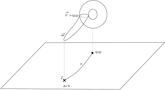
Figure 3: A membrane with boundary cycle in an elliptic fiber near a Kodaira type $I_{1}$ degeneracy. In this example, the boundary cycle is the vanishing cycle $\vec{\cal{V}}=(p,q)=(n,0)$ associated with the $I_{1}$ fiber, and $n\vec{v}$ is the homology class $\vec{J}$ of the membrane. The discriminant locus is the point in the base at which $\Delta=0$. When projected to the base, the membrane becomes the string illustrated above.

We conclude that, near a point on a smooth part of the discriminant curve with elliptic fiber of Kodaira type $I_{1}$, the $M_{4}$ worldvolume theory of a wrapped five–brane has $N=2$ supersymmetry at low energy. In addition to the “standard” Abelian Yang–Mills supermultiplet with gauge connection $A_{\mu}$ and an uncharged hypermultiplet, the $I_{1}$ degeneracy of the elliptic fiber produces a light BPS hypermultiplet

• $\Phi_{(1,0)}$   $Q_{e}=1$, $Q_{m}=0$

This electric charge couples to the gauge connection $A_{\mu}$.

The next simplest possibility, which, for example, occurs at the smooth parts of the $\sigma$ component curve, is associated with Kodaira type $I_{2}$. We will discuss this case in the next subsection.

Kodaira Type $I_{2}$:

Pick any point on the smooth part of the discriminant curve with a fiber of Kodaira type $I_{2}$, and choose the origin of the $u,v$ coordinates to be at that point. In the neighborhood of this point, the associated sections have the form

$$g_{2}=u^{0}{\cal{G}}_{2},\qquad g_{3}=u^{0}{\cal{G}}_{3},\qquad\Delta=u^{2}f^{2}$$ (4.15)

where ${\cal{G}}_{2}$, ${\cal{G}}_{3}$, and $f$, to leading order in $u$, are non–zero functions of $v$ only (see (3.30)). We see from (3.2) that the first two functions must satisfy (4.4). It follows from (3.1) and (4.15) that, at the origin, the Weierstrass form for the elliptic fiber is again given by (4.5). This is the standard Weierstrass representation of an elliptic fiber of Kodaira type $I_{2}$. As discussed above, near such a point, the $N=4$ supersymmetry of the low energy $M_{4}$ worldvolume theory of the wrapped five–brane is reduced to $N=2$ supersymmetry. This is broken to $N=1$ supersymmetry by higher dimension operators.

As above, we can restrict the discussion to the elliptic fibration ${\cal{T}}$ over the path ${\mathcal{P}}$ with coordinate $u$ that is transverse to the discriminant curve . The discriminant curve now appears as a point in the one–dimensional complex base ${\mathcal{P}}$. Furthermore, the forms of $g_{2}$, $g_{3}$ and $\Delta$, as well as the Weierstrass form of the elliptic fiber, restricted to this twofold remains those given in (4.15) and (4.5) with ${\mathcal{G}}_{2}$, ${\mathcal{G}}_{3}$ and $f$ evaluated at $v=0$. Then it follows from Table $1$ that, within ${\cal{T}}$, the degeneracy of the fiber near the discriminant point remains Kodaira type $I_{2}$.

The $SL(2,{\mathbb{Z}})$ monodromy transformation for a type $I_{2}$ fiber can be found from Table $1$, and is given by

$${\cal{M}}_{I_{2}}=\begin{pmatrix}\ 1&2\\ 0&1\end{pmatrix}.$$ (4.16)

This transformation acts on the elements of $H_{1}({\mathcal{C}}_{2},{\mathbb{Z}})$ and has, up to multiplication by a non–zero integer, the single eigenvector (4.7) with eigenvalue $+1$. At this point, however, the situation diverges substantially from that of the Kodaira type $I_{1}$ case above. This is signaled by the appearance of the 2 in the monodromy matrix, which implies that it can be decomposed as

$${\cal{M}}_{I_{2}}=\begin{pmatrix}1&1\\ 0&1\end{pmatrix}\cdot\begin{pmatrix}1&1\\ 0&1\end{pmatrix}=A\cdot A$$ (4.17)

It follows that there are now two copies of the eigenvector $\vec{{\cal{V}}}=(1,0)$ that are relevant to the problem. One way to explore this issue is to locally deform the Weierstrass equation and, hence. the discriminant in such a way that its locus, the single point at the origin with Kodaira type $I_{2}$, is split into two nearby discriminant loci, which we label $1$ and $2$, each with Kodaira type $I_{1}$. Then, the monodromy at each of these points is simply given by (4.6), with a single eigenvector (4.7). A deformation of the Weierstrass equation that will accomplish this is given by

$$y^{2}=4x^{3}-{\cal{G}}_{2}x-{\cal{G}}_{3}+u(u+\epsilon)b$$ (4.18)

Here, $b$ is the coefficient of the quadratic term in the $u$ expansion of $g_{3}$ and $\epsilon$ is a complex deformation parameter. Note, in passing, that under such a deformation a $K3$ twofold remains $K3$. The meaning of this result is the following. Consider an elliptic fiber ${\mathcal{C}}_{2}$ over a point, $z$, near, but not at, the two discriminant loci. Then the one–cycle $\vec{{\cal{V}}}=(1,0)$ is the unique cycle in $H_{1}({\mathcal{C}}_{2},\mathbb{Z})$ that contracts to zero as the fiber is moved to either of the two discriminant points. That is, $\vec{{\cal{V}}}$ is the unique vanishing cycle associated with both discriminant loci.

The physical implications arise from considering a ${\cal{T}}$–membrane whose boundary in the elliptic fiber over $z$ is $\vec{{\cal{V}}}=(1,0)$ and which “ends” on the $I_{1}$ fiber over either point $1$ or $2$ in the discriminant locus. Membranes of this type have a very specific structure. Recall that in the $I_{1}$ case above there was only one type of membrane, which ended on the unique discriminant point. In contrast, in the $I_{2}$ case there are two types of membranes, one type ending on the $I_{1}$ fiber over discriminant point $1$ and the other type ending on the $I_{1}$ fiber over discriminant point $2$. We will denote the classes associated with discriminant points $1$ and $2$ by $\vec{v_{1}}$ and $\vec{v_{2}}$ respectively. Independently of whether or not ${\cal{T}}$ is a $K3$ surface, we can show that the intersections of these membrane classes are given by

$$\vec{v_{1}}\cdot\vec{v_{1}}=\vec{v_{2}}\cdot\vec{v_{2}}=-1,\qquad\vec{v_{1}}\cdot\vec{v_{2}}=0$$ (4.19)

The proof for the self–intersections was presented in the section on $I_{1}$ and does not change here. Using the fact that $\vec{v}_{1}$ and $\vec{v}_{2}$ intersect only on the $(1,0)$ cycle in the fiber ${\mathcal{C}}_{2}$ over $z$, and that the self–intersection of this cycle vanishes, it follows that $\vec{v}_{1}\cdot\vec{v}_{2}=0$. A generic membrane of this type, projected into the base, is the string junction shown in Figure $4$. We note that the membrane intersection numbers in (4.19) are identical to the string junction lattice intersection form presented in (6.3) and (6.4) in the Appendix. Therefore, once again, we can use the membrane and string junction lattice formalism interchangeably. As the elliptic fiber approaches either of the discriminant points, the membrane fluctuations become less and less heavy, becoming exactly massless when the five–brane is wrapped on the degenerate $I_{1}$ Kodaira fiber over point $1$ or $2$. Therefore, at either of the two discriminant loci, we expect light BPS states to enter the $M_{4}$ low energy theory of the wrapped five–brane.

To compute these states, we first note that any cycle of the form $(p,0)$, where $p\in{\mathbb{Z}}$, is an eigenvector of the monodromy ${\cal{M}}_{I_{2}}$, not just $(1,0)$. The class of the associated membrane is denoted by

$$\vec{J}=n_{1}\vec{v_{1}}+n_{2}\vec{v_{2}}$$ (4.20)

where $n_{1},n_{2}\in{\mathbb{Z}}$. The boundary cycle associated with this class is given by

$$(p,q)=n_{1}(1,0)+n_{2}(1,0)$$ (4.21)

and, hence, $p=n_{1}+n_{2}$ and $q=0$. It follows from (4.19) that the self–intersection number is

$$\vec{J}\cdot\vec{J}=-n_{1}^{2}-n_{2}^{2}$$ (4.22)

However, recall that (4.13) is the condition for the associated state to be BPS saturated. In the case under consideration, since $q=0$, this condition becomes

$$\vec{J}\cdot\vec{J}\geq|n_{1}+n_{2}|-2$$ (4.23)

Comparing this with (4.22), it is clear that a state will be BPS saturated if and only if the pair $n_{1},n_{2}$ takes the values $\pm 1,0$ or $0,\pm 1$. The two BPS states described by $([1,0],[-1,0])$, combine to form a single, stable $N=2$ hypermultiplet, $\Phi^{1}_{(1,0)}$, of electric charge $Q_{e}=1$ and vanishing magnetic charge, in the $M_{4}$ worldvolume theory of the wrapped five–brane. Similarly, the states associated with $([0,1],[0,-1])$ form a second, stable $N=2$ hypermultiplet, $\Phi^{2}_{(1,0)}$, also with $Q_{e}=1$ and $Q_{m}=0$. The non-BPS states are either unstable or massive.

Figure 4: A string junction arising for a split $I_{2}$ fiber. The sum $n_{1}\vec{v}_{1}+n_{2}\vec{v}_{2}$ is the homology class $\vec{J}$ of the membrane. The boundary cycle is $(p,q)$, where $p=n_{1}+n_{2}$ and $q=0$. The vanishing cycle associated with both $\vec{v}_{1}$ and $\vec{v}_{2}$ is $(1,0)$.

Further important information can be extracted by rewriting the membrane class $\vec{J}$ in (4.20) as follows. Define classes

$$\vec{w}_{p}=\frac{1}{2}(v_{1}+v_{2}),\qquad\vec{w}=\frac{1}{2}(v_{1}-v_{2})$$ (4.24)

Then, in terms of these classes, $\vec{J}$ can be written as

$$\vec{J}=p\vec{w}_{p}+a\vec{w}$$ (4.25)

where $p=n_{1}+n_{2}$ and $a=n_{1}-n_{2}$. It is useful to proceed one step further and write this equation as

$$\vec{J}=p\vec{w}_{p}+aC^{-1}\vec{\alpha}$$ (4.26)

where $C^{-1}=\frac{1}{2}$ and $\vec{\alpha}=2\vec{w}$. Note that

$$\vec{\alpha}=v_{1}-v_{2}$$ (4.27)

which is associated with the cycle $(p,q)=(0,0)$ and, hence, corresponds to no boundary cycle at all. Such classes are described by curves from discriminant point $1$ to discriminant point $2$, as shown in Figure $5$. Furthermore, it follows from (4.19) that

$$\vec{\alpha}\cdot\vec{\alpha}=-2$$ (4.28)

We see, by comparing equations (4.26) and (4.27) with (6.6) and (6.7) in the Appendix, that class $\vec{\alpha}$ corresponds to the simple root of the Lie algebra of $SU(2)$.

Figure 5: The junction corresponding to the simple root of $SU(2)$.

Note that, written as a pair $[n_{1},n_{2}]$, class $\vec{\alpha}=[1,-1]$. It follows that the BPS states that make up the hypermultiplet $\Phi^{1}_{(1,0)}$, specified by $[1,0]$ and $[-1,0]$, are related to the BPS states, $[0,1]$ and $[0,-1]$, that make up the hypermultiplet $\Phi^{2}_{(1,0)}$ through addition and subtraction of the root vector $\vec{\alpha}$. That is

$$[1,0]-\vec{\alpha}=[0,1],\qquad[-1,0]+\vec{\alpha}=[0,-1]$$ (4.29)

Further addition and subtraction of the root $\vec{\alpha}$ leads to unstable or massive non–BPS states. It follows that hypermultiplets $\Phi^{1}_{(1,0)}$ and $\Phi^{2}_{(1,0)}$ form a doublet representation of $SU(2)$. The appearance of an $SU(2)$ global group can be read off directly from the A-D-E column of Table $1$. For Kodaira type $I_{2}$, the A-D-E classification is $A_{1}$, which corresponds to the group $SU(2)$.

We conclude that, near a point on a smooth part of the discriminant curve with elliptic fiber of Kodaira type $I_{2}$, the $M_{4}$ worldvolume theory of a wrapped five–brane has $N=2$ supersymmetry at low energy. In addition to the “standard” Abelian Yang–Mills supermultiplet with gauge connection $A_{\mu}$ and an uncharged hypermultiplet, the $I_{2}$ degeneracy of the elliptic fiber produces an $SU(2)$ doublet ${\bf 2\rm}$ of light BPS hypermultiplets

• $\Phi^{i}_{(1,0)}$   $Q_{e}=1,Q_{m}=0$

where $i=1,2$. The electric charge couples to the gauge connection $A_{\mu}$.

We now turn our attention to more a more complicated situation, specifically that of a Kodaira type $IV$ fiber occuring at the smooth part of the discriminant curve. Such fibers are found, for example, over the smooth part of the component curve ${\mathcal{S}}$ in Case $3$ above. The analysis of this example contains most of the elements necessary to compute the light BPS states for a fiber of any Kodaira type over a smooth part of the discriminant curve.

Kodaira Type IV:

Pick any point on the smooth part of the discriminant curve with a fiber of Kodaira type $IV$, and choose the origin of the $u,v$ coordinates to be at that point. In the neighborhood of this point, the associated sections have the form

$$g_{2}=u^{L}{\cal{G}}_{2},\qquad g_{3}=u^{2}{\cal{G}}_{3},\qquad\Delta=u^{4}f^{2}$$ (4.30)

where $L>1$ and ${\cal{G}}_{2}$, ${\cal{G}}_{3}$ and $f$, to leading order in $u$, are non–vanishing functions of $v$ only. Further analysis of the explicit curve ${\mathcal{S}}$ in Case $3$ above fixes the value of coefficient $L$ to be $L=2$. We see from (3.2) that, near the discriminant locus,

$$\Delta=g_{2}^{3}-27g_{3}^{2}=u^{4}(-27{\cal{G}}_{3}^{2})$$ (4.31)

which vanishes at the locus without any further restrictions on ${\cal{G}}_{2}$ and ${\cal{G}}_{3}$. It follows from (3.1) and (4.30) that, at the origin, the Weierstrass form of the elliptic fiber becomes

$$y^{2}=4x^{3}-u^{2}{\cal{G}}_{2}x-u^{2}{\cal{G}}_{3}$$ (4.32)

where we have used affine coordinates with $z=1$. This is the Weierstrass representation of an elliptic fiber of Kodaira type $IV$. Near such a point, the $N=4$ supersymmetry of the low energy $M_{4}$ worldvolume theory of the wrapped five–brane is reduced to $N=2$ supersymmetry. This is broken to $N=1$ supersymmetry by higher dimensional operators.

As above, we can restrict the discussion to the elliptic fibration over the path ${\mathcal{P}}$ with coordinate $u$ that is transverse to the discriminant curve . The discriminant curve now appears as a point in the one–dimensional complex base ${\mathcal{P}}$. The forms of $g_{2}$, $g_{3}$ and $\Delta$, as well as the Weierstrass form of the elliptic fiber, restricted to this twofold remain those given in (4.30) and (4.32) with ${\mathcal{G}}_{2}$, ${\mathcal{G}}_{3}$ and $f$ evaluated at $v=0$. It follows from Table $1$ that, within ${\cal{T}}$, the degeneracy of the fiber near the discriminant point remains that of Kodaira type $IV$.

The $SL(2,{\mathbb{Z}})$ monodromy transformation for a type $IV$ fiber can be found from Table $1$. Here, for technical reasons, it is convenient to use a monodromy matrix conjugate to the one listed in Table $1$ given by

$${\cal{M}}_{IV}=\begin{pmatrix}-1&1\\ -1&0\end{pmatrix}$$ (4.33)

This transformation acts on the elements of $H_{1}({\mathcal{C}}_{2},{\mathbb{Z}})$. However, unlike the previous cases of Kodaira type $I_{1}$ and $I_{2}$, ${\cal{M}}_{IV}$ has no real eigenvector and, therefore, there is no obvious associated vanishing cycle. An indication as how to proceed is given by the fact that ${\cal{M}}_{IV}$ can be decomposed as

$${\cal{M}}_{IV}=\begin{pmatrix}1&1\\ 0&1\end{pmatrix}\cdot\begin{pmatrix}1&1\\ 0&1\end{pmatrix}\cdot\begin{pmatrix}1&1\\ 0&1\end{pmatrix}\cdot\begin{pmatrix}2&1\\ -1&0\end{pmatrix}=A\cdot A\cdot A\cdot B$$ (4.34)

Following the technique employed in the $I_{2}$ case, we proceed by deforming the discriminant curve in such a way that its locus, the single point at the origin with Kodaira type $IV$, is split into four nearby discriminant points, which we label $1$,$2$,$3$ and $4$. This corresponds to a relevant deformation of the Weierstrass representation given by

$$y^{2}=4x^{3}-u^{2}{\cal{G}}_{2}x-u^{2}{\cal{G}}_{3}+\epsilon$$ (4.35)

where $\epsilon$ is a constant deformation parameter. The first three points each have a Kodaira fiber of type $I_{1}$ with the monodromy given in (4.6) and, up to multiplication by a non–zero integer, the single eigenvector (4.7). The fourth point, however, has monodromy

$$B=\begin{pmatrix}2&1\\ -1&0\end{pmatrix}$$ (4.36)

with, up to multiplication by a non–zero integer, the eigenvector

$$\vec{\tilde{\cal{V}}}=(1,-1)$$ (4.37)

At first glance, it is not obvious what Kodaira type one is finding in this last case. However, it is easy to show that $A$ is, in fact, conjugate to $B$ and, hence, the fiber at point $4$ is also of Kodaira type $I_{1}$. The meaning of these results is the following. Consider an elliptic fiber ${\mathcal{C}}_{2}$ over a point, $z$, near, but not at, the four discriminant loci. Then the one–cycle $\vec{{\cal{V}}}=(1,0)$ is the unique cycle in $H_{1}({\mathcal{C}}_{2},\mathbb{Z})$ that contracts to zero as the fiber is moved to each of the discriminant points $1$, $2$, and $3$ without encircling $4$. That is, $\vec{{\cal{V}}}$ is the unique vanishing cycle associated with the first three discriminant loci. Similarly, the one–cycle $\vec{\tilde{\cal{V}}}=(1,-1)$ is the unique cycle in $H_{1}({\mathcal{C}}_{2},\mathbb{Z})$ that contracts to zero as the fiber is moved to the discriminant point $4$ without encircling $1,\ 2$ or $3$. That is, $\vec{\tilde{\cal{V}}}$ is the unique vanishing cycle associated with the fourth discriminant locus.

The physical implications of this arise as follows. ${\cal{T}}$– membranes that are bounded by the vanishing cycle $\vec{{\cal{V}}}=(1,0)$ in the elliptic fiber over $z$ are of a very specific structure. There are three membranes of this type, each “ending” on the $I_{1}$ fiber over discriminant points $1$,$2$ or $3$ respectively. Similarly, membranes that are bounded by the vanishing cycle $\vec{\tilde{\cal{V}}}=(1,-1)$ have a very specific structure. These membranes “end” on the $I_{1}$ fiber over the discriminant point $4$. We will denote the ${\cal{T}}$–membrane classes associated with discriminant points $1$, $2$,$3$ and $4$ by $\vec{v_{1}}$,$\vec{v_{2}}$, $\vec{v_{3}}$ and $\vec{v_{4}}$ respectively. A generic membrane class of this type, projected into the base, is the string junction shown in Figure $6$. Note from the Appendix that the intersections of these membrane classes are given by

$$\vec{v_{1}}\cdot\vec{v_{1}}=\vec{v_{2}}\cdot\vec{v_{2}}=\vec{v_{3}}\cdot\vec{v_{3}}=\vec{v_{4}}\cdot\vec{v_{4}}=-1$$ (4.38)

$$\vec{v_{1}}\cdot\vec{v_{2}}=\vec{v_{1}}\cdot\vec{v_{3}}=\vec{v_{2}}\cdot\vec{v_{3}}=0$$ (4.39)

$$\vec{v_{1}}\cdot\vec{v_{4}}=\vec{v_{2}}\cdot\vec{v_{4}}=\vec{v_{3}}\cdot\vec{v_{4}}=-\frac{1}{2}$$ (4.40)

As the elliptic fiber approaches any one of the discriminant points, the membrane fluctuations become less and less heavy, becoming exactly massless when the five–brane is wrapped on the degenerate $I_{1}$ Kodaira fiber over point $1$,$2$,$3$ or $4$. Therefore, at any of the four discriminant loci, we expect light BPS states to enter the $M_{4}$ low energy theory of the wrapped five–brane.

To compute these states, we first note, by analogy with the above discussion, that the classes of the associated membranes are given by

$$\vec{J}=\Sigma^{4}_{i=1}n_{i}\vec{v_{i}}$$ (4.41)

where $n_{i}$, $i=1,..,4$ are arbitrary integers. Using (4.7) and (4.37), it follows that the associated boundary cycles in $H_{1}({\mathcal{C}}_{2},\mathbb{Z})$ are given by

$$(p,q)=\Sigma_{i=1}^{3}n_{i}(1,0)+n_{4}(1,-1)$$ (4.42)

and, hence, $p=\Sigma_{i=1}^{4}n_{i}$ and $q=-n_{4}$. From (4.39), we find that the self–intersection number of class $\vec{J}$ is

$$\vec{J}\cdot\vec{J}=-\Sigma_{i=1}^{4}n_{i}^{2}-(n_{1}+n_{2}+n_{3})n_{4}$$ (4.43)

However, recall that (4.13) is the condition for the associated state to be BPS saturated. Comparing this to (4.43), it was shown in [26, 27] that a state will be BPS saturated if and only if $n_{1},n_{2},n_{3},n_{4}$ take the values

$(n_{1},n_{2},n_{3},n_{4})$	$(p,q)$
$(1,0,0,0),(0,1,0,0),(0,0,1,0)$	$(1,0)$
$(-1,0,0,0),(0,-1,0,0),(0,0,-1,0)$	$(-1,0)$
$(1,0,0,-1),(0,1,0,-1),(0,0,1,-1)$	$(0,1)$
$(-1,0,0,1),(0,-1,0,1),(0,0,-1,1)$	$(0,-1)$
$(0,-1,-1,1),(-1,0,-1,1),(-1,-1,0,1)$	$(-1,-1)$
$(0,1,1,-1),(1,0,1,-1),(1,1,0,-1)$	$(1,1)$
$(1,1,1,-2)$	$(1,2)$
$(-1,-1,-1,2)$	$(-1,-2)$
$(0,0,0,1)$	$(1,-1)$
$(0,0,0,-1)$	$(-1,1)$
$(1,1,1,-1)$	$(2,1)$
$(-1,-1,-1,1)$	$(-2,-1)$

Table 2: The BPS states associated with a fiber of Kodaira type $IV$.

The six BPS states in the first row combine to form a triplet of $N=2$ hypermultiplets, each of electric charge $Q_{e}=1$ and vanishing magnetic charge, in the $M_{4}$ worldvolume theory of the wrapped five–brane. We denote these hypermultiplets by $\Phi_{(1,0)}^{i}$, where $i=1,2,3$. Similarly, the second and third rows each correspond to a triplet of $N=2$ hypermultiplets, which we denote by $\Phi_{(0,1)}^{i}$ and $\Phi_{(-1,-1)}^{i}$ with $i=1,2,3$ respectively. As indicated by the notation, the multiplet $\Phi_{(0,1)}^{i}$ has vanishing electric charge and magnetic charge $Q_{m}=1$, whereas $\Phi_{(-1,-1)}^{i}$ carries both electric charge $Q_{e}=-1$ and magnetic charge $Q_{m}=-1$. The two BPS states in the fourth row combine to form a single, $N=2$ hypermultiplet, $\Psi_{(1,2)}$ with $Q_{e}=1$ and $Q_{m}=2$. Finally, the last two rows each correspond to a single $N=2$ hypermultiplet, denoted by $\Psi_{(1,-1)}$ and $\Psi_{(2,1)}$, with $Q_{e}=1$, $Q_{m}=-1$ and $Q_{e}=2$, $Q_{m}=1$ respectively. The non–BPS states are either unstable or massive. When the deformation that split the $IV$ fiber is undone, all these BPS multiplets become simultaneously massless as the fivebrane is moved towards the $IV$ fiber. These states have mutually non-local $(p,q)$ charges, meaning that they can not be made simultaneously purely electric by an $SL(2,{\mathbb{Z}})$ transformation. This leads to a very exotic low energy theory without a local Lagrangian description. Such theories were obtained originally, in a different context, in [31, 32, 33]. When the fivebrane wraps the type $IV$ Kodaira fiber, the low energy theory flows to an interacting fixed point in the infrared.

Figure 6: A string junction for a split type IV Kodaira fiber. The sum $\sum_{i=1}^{4}n_{i}\vec{v}_{i}$ is the homology class $\vec{J}$ of the membrane, and $(p,q)$ is the boundary cycle. In this case $p=\sum_{i=1}^{4}n_{i}$ and $q=-n_{4}$ The vanishing cycle associated with $\vec{v}_{1},\vec{v}_{2}$ and $\vec{v}_{3}$ is $(1,0)$, while that of the $\vec{v}_{4}$ is $(1,-1)$.

Further important information can be extracted by rewriting the membrane class $\vec{J}$ as follows. Define classes

$$\vec{w}_{p}=\frac{1}{3}(v_{1}+v_{2}+v_{3}),\qquad\vec{w}_{q}=\frac{1}{3}(v_{1}+v_{2}+v_{3})-v_{4}$$ (4.44)

and

$$\vec{w}^{1}=\frac{1}{3}(2v_{1}-v_{2}-v_{3}),\qquad\vec{w}^{2}=\frac{1}{3}(v_{1}+v_{2}-2v_{3})$$ (4.45)

Then, in terms of these classes, $\vec{J}$ can be written as

$$\vec{J}=p\vec{w}_{p}+q\vec{w}_{q}+a_{i}\vec{w}^{i}$$ (4.46)

where $p$ and $q$ are given in (4.42) and

$$a_{1}=n_{1}-n_{2},\qquad a_{2}=n_{2}-n_{3}$$ (4.47)

It is useful to proceed one step further and write equation (4.46) as

$$\vec{J}=p\vec{w}_{p}+q\vec{w}_{q}+a_{i}C^{-1ij}\vec{\alpha}_{i}$$ (4.48)

where $\vec{\alpha}_{1}=2w^{1}-w^{2}$, $\vec{\alpha}_{2}=-w^{1}+2w^{2}$ and $C_{ij}=-\vec{\alpha}_{i}\cdot\vec{\alpha}_{j}$. Note that

$$\vec{\alpha}_{1}=v_{1}-v_{2},\qquad\vec{\alpha}_{2}=v_{2}-v_{3}$$ (4.49)

which are both associated with the cycle $(p,q)=(0,0)$ and, hence, each corresponds to no boundary cycle at all. Therefore, $\vec{\alpha}_{1}$ is described by curves from discriminant point $1$ to discriminant point $2$ and $\vec{\alpha}_{2}$ is described by curves from discriminant point $2$ to discriminant point $3$, as shown in Figure $6$. Furthermore, it follows from (4.39) that

$$C_{ij}=\begin{pmatrix}2&-1\\ -1&2\end{pmatrix}$$ (4.50)

which is the Cartan matrix of the Lie algebra of $SU(3)$. Hence, the classes $\vec{\alpha}_{1}$ and $\vec{\alpha}_{2}$ correspond to the simple roots of the $SU(3)$. Note that, written as a four–tuplet $[n_{1},n_{2},n_{3},n_{4}]$, class $\vec{\alpha}_{1}=[1,-1,0,0]$ and class $\vec{\alpha}_{2}=[0,1,-1,0]$.

Figure 7: The two simple roots of $SU(3)$, realized as string junctions for the split Kodaira type IV fiber. Note that there are no root junctions with an endpoint on the fourth $I_{1}$ fiber.

Consider, for example, the six BPS states in the first row of Table $2$, and note that

$$[1,0,0,0]-\vec{\alpha}_{1}=[0,1,0,0],\qquad[0,1,0,0]-\vec{\alpha}_{2}=[0,0,1,0]$$ (4.51)

$$[-1,0,0,0]+\vec{\alpha}_{1}=[0,-1,0,0],\qquad[0,-1,0,0]+\vec{\alpha}_{2}=[0,0,-1,0]$$ (4.52)

Further addition or subtraction of the roots leads to non–BPS states that are either unstable or massive. Hence, the pairs of BPS states $([1,0,0,0],[-1,0,0,0])$, $([0,1,0,0],[0,-1,0,0])$ and $([0,0,1,0],[0,0,-1,0])$ combine to form the hypermultiplets $\Phi_{(1,0)}^{1},\Phi_{(1,0)}^{2}$ and $\Phi_{(1,0)}^{3}$ respectively. Furthermore, these hypermultiplets form a triplet $\bf 3\rm$ representation of $SU(3)$. The same is true for the hypermultiplets $\Phi_{(0,1)}^{i}$ and $\Phi_{(-1,-1)}^{i}$ for $i=1,2,3$, each of which transforms as an $SU(3)$ $\bf 3\rm$ representation. Now consider the two BPS states in the fourth row of Table $2$. Addition or subtraction of any root leads immediately to non–BPS states which are either unstable of massive. Hence, the pair of BPS states $([1,1,1,-2],[-1,-1,-1,2])$ combine to form a hypermultiplet $\Psi_{(1,2)}$, which is a singlet under $SU(3)$. The same is true for $\Psi_{(1,-1)}$ and $\Psi_{(2,1)}$ which are both $SU(3)$ singlets. The appearance of the global group $SU(3)$ can be read off directly from the A-D-E column of Table $1$. For Kodaira type $IV$, the A-D-E classification is $A_{2}$, which corresponds to the group $SU(3)$.

We conclude that, near a point on a smooth part of the discriminant curve with elliptic fiber of Kodaira type $IV$, the $M_{4}$ worldvolume theory of a wrapped five–brane has $N=2$ supersymmetry at low energy. In addition to the “standard” Abelian Yang–Mills supermultiplet with gauge connection $A_{\mu}$ and an uncharged hypermultiplet, the $IV$ degeneracy of the elliptic fiber produces light BPS hypermultiplets. These fall into $SU(3)$ $\bf 3\rm$ representations

• $\Phi_{(1,0)}^{i}$   $Q_{e}=1,Q_{m}=0$

• $\Phi_{(0,1)}^{i}$   $Q_{e}=0,Q_{m}=1$

• $\Phi_{(-1,-1)}^{i}$   $Q_{e}=-1,Q_{m}=-1$

with $i=1,2,3$ and $SU(3)$ singlets

• $\Psi_{(1,2)}$   $Q_{e}=1,Q_{m}=0$

• $\Psi_{(1,-1)}$   $Q_{e}=1,Q_{m}=-1$

• $\Psi_{(2,1)}$   $Q_{e}=2,Q_{m}=1$

The electric charge couples to gauge connection $A_{\mu}$ whereas the magnetic charge couples to $\tilde{A_{\mu}}$ defined by $d\tilde{A_{\mu}}=*F$.

We end this section by presenting the BPS states associated with each of the remaining Kodaira types, $I_{0}^{*}$ ,$III^{*}$, and $IV^{*}$, over the smooth parts of the discriminant curve in the $B=\hat{\mathbb{F}}_{3}$ model.

Kodaira Types $I_{0}^{*}$, $III^{*}$, and $IV^{*}$:

The A-D-E symmetry algebra associated with a fiber of Kodaira type $I_{0}^{*}$ can be read off from Table $1$ and is given by $D_{4}$. The associated global symmetry group is $SO(8)$. The low energy theory that arises in the neighborhood of an $I_{0}^{*}$ fiber is the same as that of an $N=2$, $SU(2)$ Yang–Mills theory with four quark flavors. The BPS multiplets in the $I_{0}^{*}$ case can be easily found by comparing to Yang-Mills theory results [29, 30], or by using string junctions as in [27]. The results are summarized in the table below.

$(p,q)$ charges	$SO(8)$ representation
$(2n,2m)$	${\bf 1\rm}$
$(2n+1,2m)$	${\bf 8_{v}\rm}$
$(2n,2m+1)$	${\bf 8_{s}\rm}$
$(2n+1,2m+1)$	${\bf 8_{c}\rm}$

Table 3: The BPS multiplets associated with a fiber of Kodaira type $I_{0}^{*}$.

Table $3$ is to be read as follows. For each $n$ and $m$, there is an $N=2$ multiplet with the $(p,q)$ charges listed in the first column, which transforms in the representation of $SO(8)$ listed in the last column. In the first row, $n$ and $m$ are constrained to be relatively prime, whereas in the remaining rows, $p$ and $q$ must be relatively prime. There are no further constraints. Note that, in analogy to the Kodaira type $IV$ case, there are a finite number of representations of $SO(8)$ which appear, specifically singlets and octets only. However, unlike the type $IV$ case, each of these representations occurs with infinite multiplicity. Of course not all of these multiplets are simultaneously stable, depending on the location of the five–brane in moduli space.

Let us summarize these results in terms of $N=2$ supermultiplets. In addition to the “standard” Abelian vector supermultiplet with gauge connection $A_{\mu}$ and an uncharged hypermultiplet, the $I_{0}^{*}$ degeneracy of the elliptic fiber produces light BPS hyper- and vector multiplets. The extra vector multiplets are $SO(8)$ singlets with $p=\pm 2$ and $q=0$

• $V_{\pm}$

As the five–brane approaches the discriminant curve, these combine with the usual uncharged Abelian vector multiplet to form massless $N=2$ vector multiplets $V_{a}$ which transform as the adjoint representation of an enhanced $SU(2)$ gauge group. The remaining states belong to hypermultiplets

• $\Phi^{i}_{(p,q)}$   $Q_{e}=p$, $Q_{m}=q$

where the charges $(p,q)$ and the $SO(8)$ representation multiplets $i$ are given in Table $3$. As the five–brane approaches the discriminant curve, the hypermultiplets transforming as ${\bf 8_{v}\rm}$ under $SO(8)$ with $q=0$ combine to form an $SU(2)$ doublet ${\bf 2\rm}$, $Q^{i}_{A}$, where $i$ is the index of the ${\bf 8_{v}\rm}$ representation and $A=1,2$. These correspond to hypermultiplets of four $SU(2)$ doublet quark flavors.

The A-D-E symmetry algebras associated with fibers of Kodaira type $III^{*}$ and $IV^{*}$ can be read off from Table $1$. The associated global symmetry groups are the exceptional groups $E_{7}$ and $E_{6}$ respectively. The complete spectrum of BPS multiplets for these two Kodaira types are much harder to determine, for reasons discussed below, and we will present only partial results [27]. First, note from Table $4$ in the Appendix that the monodromy associated with a Kodaira fiber of type $I_{0}^{*}$ decomposes into type $I_{1}$ monodromies as $AAAABC$. Similarly, one sees that Kodaira fibers of type $III^{*}$ and $IV^{*}$ decompose as $AAAAAABCC$ and $AAAAABCC$ respectively. It follows that the $I_{0}^{*}$ string junction lattice is a sublattice of the $III^{*}$ and $IV^{*}$ junction lattices. This reflects the fact that a fiber of type $I_{0}^{*}$ may be obtained from type $III^{*}$ or type $IV^{*}$ fibers by deformations of the discriminant curve; one simply moves some of the $I_{1}$ fibers in the decomposition of the $III^{*}$ or $IV^{*}$ to infinity, leaving only the $I_{1}$ fibers which make up the $I_{0}^{*}$. For instance, the $IV^{*}$ fiber decomposes into $I_{1}$ fibers of monodromy type AAAAABCC. By moving one $I_{1}$ of type A and another of type $C$ to infinity, one is left with $I_{1}$ fibers of monodromy type AAAABC, which is the decomposition of an $I_{0}^{*}$ fiber. It follows from this that each of the $I_{0}^{*}$ BPS multiplets listed in Table $3$ is also a BPS multiplet of both the Kodaira type $III^{*}$ and type $IV^{*}$ fibers. However, it turns out that $I_{0}^{*}$ multiplets with different $(p,q)$ charges transforming in the same representation of $SO(8)$, transform as different representations of the exceptional groups of the Kodaira fibers $III^{*}$ and $IV^{*}$. For example [27], the ${\bf 8_{v}\rm}$ appearing for the $I_{0}^{*}$ fiber with charges $(p,q)=(1,0)$ is embedded in a ${\bf 56\rm}$ of $E_{7}$, or a ${\bf 27\rm}$ of $E_{6}$, while the ${\bf 8_{v}\rm}$ with charges $(p,q)=(1,2)$ is embedded in a ${\bf 27664\rm}$ of $E_{7}$, or a ${\bf 351\rm}$ of $E_{6}$. Consequently, although the type $I_{0}^{*}$ BPS multiplets with $(p,q)$ charges listed in Table $3$ are also BPS multiplets of type $III^{*}$ and type $IV^{*}$ fibers, they are classified by an infinite number of different $E_{7}$ and $E_{6}$ representations. Although these can be computed on a case by case basis, a simple listing of such multiplets is impossible. In addition, there are BPS multiplets associated with both type $III^{*}$ and type $IV^{*}$ fibers that are unrelated to those of the $I_{0}^{*}$. These multiplets arise from string junctions involving the type $A$ and type $C$ $I_{1}$ fibers not contained in the decomposition of $I_{0}^{*}$. We will not discuss these states here, referring the interested reader to [27]. Again, one expects BPS states with mutually non-local charges to become simultaneously massless as the five-brane approaches the singular fiber. The low energy theory on the five-brane wrapping the singular fiber flows to an exotic interacting fixed point theory. The fixed point theories with exceptional global symmetries were first discussed, in a different context, in [33].

5 Conclusion:

In this paper, we have presented detailed techniques for computing the discriminant curves of elliptically fibered Calabi–Yau threefolds. These were applied to a specific three–family, $SU(5)$ GUT model of particle physics within the context of Heterotic M–Theory. In this theory, and in general, the discriminant curves have an intricate structure, consisting of smooth sections, cusps and tangential and normal self–intersections. The type of degeneration of the elliptic fiber, classified by Kodaira, changes in the different regions of the discriminant curve. In this paper, we discussed how to find the Kodaira type of the fiber singularities and explicitly computed them for the discriminant curves associated with the $SU(5)$ GUT model. In Heterotic M–Theory, anomaly cancellation generically requires the existence of five–branes, located in the bulk space, wrapped on a holomorphic curve in the associated Calabi–Yau threefold. We showed that there is always a region of the moduli space of this holomorphic curve that corresponds a single five–brane wrapped on a pure fiber elliptic curve. Since this fiber degenerates as it approaches the discriminant curve, one expects light BPS states to appear in the worldvolume theory of this five–brane. For points on the smooth parts of the discriminant curve, we demonstrated in detail how the M–theory membranes associated with these states are, when projected into the base space, related to string junction lattices. Using string junction techniques, we computed the massless BPS hyper- and vector multiplets for all the Kodaira type degeneracies that occur in our specific $SU(5)$ GUT model. The Kodaira theory, as well as the computation of light states, is considerably more intricate at the cusp and self–intersection points of the discriminant curve. These topics will be discussed in a forthcoming publication.

It is important to note that the solutions of the BPS constraint on string junctions only gives a list of the possible BPS states in the spectrum. Determining their stability at different points in moduli space is a dynamical question, and the answer is not completely known for the exceptional Kodaira types. The answer is known for the non–exceptional Kodaira degeneracies, including the types $I_{1}$, $I_{2}$, $IV$ and $I_{0}^{*}$ discussed in this paper [29, 30]. In the $I_{0}^{*}$ case, the states listed in Table $3$ all appear in the stable spectrum at different points in moduli space. It follows that the multiplets of the exceptional groups $E_{7}$ and $E_{6}$ into which these states are embedded also exist in the spectrum. However, nothing is known about the stability of the multiplets which decouple upon deforming the exceptional fibers into $I_{0}^{*}$.

Acknowledgements

We would like to thank P. Candelas, D. Luest, D. Morrison and B. Zwiebach for useful conversations and discussions. B. Ovrut is supported in part by a Senior Alexander von Humboldt Award, by the DOE under contract No. DE-ACO2-76-ER-03071 and by the University of Pennsylvania Research Foundation Grant. Z. Guralnick is supported in part by the DOE under contract No. DE-ACO2-76-ER-03071. A. Grassi is supported in part by an NSF grant DMS-9706707.

6 Appendix A– Review of String Junctions:

This Appendix contains a review of string junctions, and is a brief summary of work found in [26, 27]. There, string junctions were discussed in the context of type IIB string theory on ${\mathbb{CP}}^{1}$. As described in this paper, membrane junctions in an elliptically fibered surface in M–theory become string junctions when projected into the base.

The equivalence classes of string junctions form a lattice with a quadratic form. To define the junction lattice, one initially splits all Kodaira fibers into a number of type $I_{1}$ fibers by a suitable deformation of the Weierstrass model (a “relevant deformation”). The string junctions lie in the base space. The $I_{1}$ loci are points in the base and the string junctions start from a fixed point $P$ away from these loci and may end only at the $I_{1}$ points. Each segment of the junction is an oriented string with charges $(p,q)$, which are conserved at branching points. The charges $(p,q)$ correspond to a one–cycle in the associated elliptic fiber $F$ over the point $P$. The segment of a string junction ending at an $I_{1}$ locus has charges which are proportional to the vanishing cycle $(p_{i},q_{i})$ for the $i$-th $I_{1}$ fiber. The vanishing cycle is the eigenvector of the monodromy matrix

$${\mathcal{M}}_{i}=\begin{pmatrix}1-p_{i}q_{i}&p^{2}_{i}\\ -q_{i}^{2}&1+p_{i}q_{i}\end{pmatrix}$$ (6.1)

In a convenient decomposition [26], any Kodaira fiber may be split into $I_{1}$ fibers on the real axis each with vanishing cycles $(1,0)$, $(1,-1)$, or $(1,1)$. The associated monodromy matrices are, using (6.1), given by

$$A=\begin{pmatrix}1&1\\ 0&1\end{pmatrix},\qquad B=\begin{pmatrix}2&1\\ -1&0\end{pmatrix},\qquad C=\begin{pmatrix}0&1\\ -1&2\end{pmatrix}$$ (6.2)

respectively. The decompositions of the general Kodaira type fibers into $I_{1}$ fibers, from left to right on the real axis, are listed below.

Kodaira type	decomposition
$I_{n}$	$A^{n}$
$II$	$AB$
$III$	$AAB$
$IV$	$AAAB$
$I_{n}^{*}$	$A^{4+n}BC$
$IV^{*}$	$AAAAABCC$
$III^{*}$	$AAAAAABCC$
$II^{*}$	$AAAAAAABCC$

Table 4: The decomposition of Kodaira fibers into type $I_{1}$ fibers and the associated monodromy.

The basis cycles on the elliptic fiber are not globally defined, and there are branch cuts which may be taken to extend vertically downward from each $I_{1}$ loci. As a segment of the string junction crosses the branch cut of the $i$-th $I_{1}$ locus, the $(p_{i},q_{i})$ charges labeling the cycle over this segment are acted on by the monodromy ${\mathcal{M}}_{i}$. Such a segment can be pulled across the $I_{1}$ locus so that it no longer crosses the branch cut. However, because of a Hanany-Witten effect, an additional segment appears stretching between the original segment and the $I_{1}$ locus, as illustrated in Figure $8$. The charges of the new segment are determined by charge conservation to be $(p^{\prime},q^{\prime})={\mathcal{M}}_{i}(p,q)-(p,q)$, which is proportional to the vanishing cycle $(p_{i},q_{i})$. The two junctions related by pulling this segment across the $I_{1}$ locus are equivalent. Thus, the equivalence classes of junctions can be determined by considering only junctions which have no components below the real axis, as in Figure $8(b)$. The equivalence classes are then labeled by vectors $\vec{J}=\sum_{i}n_{i}\vec{v}_{i}$, where the integers $n_{i}$ indicate that the charges of the segment ending on the $i$-th $I_{1}$ locus are $n_{i}(p_{i},q_{i})$. The dimension of the string junction lattice is equal to the number of $I_{1}$ fibers. The reader is referred to [26] for details on the construction of the quadratic intersection form on the junction lattice. Here, we simply state the results. The intersection form is given by

$$\vec{v}_{i}\cdot\vec{v}_{i}=-1$$ (6.3)

$$\vec{v}_{i}\cdot\vec{v}_{j}=\frac{1}{2}(p_{i}q_{j}-q_{i}p_{j}),\quad i\neq j$$ (6.4)

The basis in which an equivalence class $\vec{J}$ is labeled by the integers $n_{i}$ is not the most useful one. There is another basis in which the gauge and global symmetry charges appear explicitly. Viewed as quantum numbers of a BPS state, the electric and magnetic charges of a string junction are $(p,q)=\sum_{i}n_{i}(p_{i},q_{i})$. The remaining directions in the lattice are related to global symmetry charges. Using the intersection form on the lattice, one can show that the junction lattice contains the weight lattice of a (simply laced) Lie algebra [26]. The simple roots of the Lie algebra correspond to a basis set of string junctions with vanishing charges $(p,q)=(0,0)$, and have self–intersection $-2$. The intersection matrix of the simple root junctions $\vec{\alpha}_{i}$ is minus the Cartan matrix of the Lie algebra

$$\vec{\alpha}_{i}\cdot\vec{\alpha}_{j}=-C_{ij}.$$ (6.5)

When $I_{1}$ fibers coalesce to form another Kodaira fiber, some root junctions have vanishing length. The Lie algebra associated with these simple roots generates a global symmetry of the theory which matches the A-D-E type of the Kodaira fiber. Fundamental weight junctions $\vec{w}^{i}$ with vanishing $(p,q)$ charges are defined by $\vec{w}^{i}\cdot\vec{\alpha}_{j}=-\delta^{i}_{j}$, and are related to the simple root junctions by

$$\vec{w}^{i}=C^{-1ij}\vec{\alpha}_{j}.$$ (6.6)

The fundamental weight junctions are “improper” in the sense that the $n_{i}$ associated with them are not integers. To get a complete basis, one defines another pair of string junctions $\vec{w}_{p}$ and $\vec{w}_{q}$. These are orthogonal to the fundamental weight junctions $\vec{w}^{i}$ and carry total charges $(p,q)=(1,0)$ and $(0,1)$ respectively. The junctions $\vec{w}_{p}$ and $\vec{w}_{q}$ are also improper. Any proper junction $\vec{J}$ can be written as

$$\vec{J}=p\vec{w}_{p}+q\vec{w}_{q}+a_{i}\vec{w}^{i}.$$ (6.7)

where the integers $a_{i}$ are the Dynkin labels. The weights in a BPS representation consist of junctions $\vec{J}$ related by the addition of simple roots, and satisfying the BPS condition [27, 28]

$$\vec{J}\cdot\vec{J}\geq-2+gcd(p,q),$$ (6.8)

where $gcd$ denotes the greatest common positive divisor of $p$ and $q$.

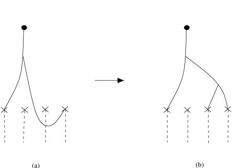
Figure 8: Two equivalent string junction lattices. The dashed lines indicate branch cuts.

References

- [1] A. Lukas, B. A. Ovrut, K. S. Stelle and D. Waldram, The Universe as a Domain Wall, Phys.Rev. D59 (1999) 086001; Heterotic M-theory in Five Dimensions, Nucl.Phys. B552 (1999) 246-290.
- [2] A. Lukas, B. A. Ovrut and D. Waldram, Non-Standard Embedding and Five-Branes in Heterotic M-Theory, Phys.Rev. D59 (1999) 106005.
- [3] R. Donagi, A. Lukas, B. A. Ovrut and D. Waldram, Non-Perturbative Vacua and Particle Physics in M-Theory, JHEP 9905 (1999) 018; Holomorphic Vector Bundles and Non-Perturbative Vacua in M-Theory, JHEP 9906 (1999) 034.
- [4] A. Lukas, B. A. Ovrut and D. Waldram, Five–Branes and Supersymmetry Breaking in M–Theory, JHEP 9904 (1999) 009.
- [5] R. Donagi, B. A. Ovrut and D. Waldram, Moduli Spaces of Fivebranes on Elliptic Calabi-Yau Threefolds, JHEP 9911 (1999) 030.
- [6] R. Donagi, B. A. Ovrut, T. Pantev and D. Waldram, Standard Models from Heterotic M-theory, hep-th/9912208.
- [7] B. A. Ovrut, T. Pantev and J. Park, Small Instanton Transitions in Heterotic M-Theory, hep-th/0001133.
- [8] P. Hořava and E. Witten, Heterotic and Type I String Dynamics from Eleven Dimensions, Nucl. Phys. B460(1996) 506; Eleven–Dimensional Supergravity on a Manifold with Boundary, Nucl. Phys. B475(1996) 94.
- [9] N. Arkani-Hamed, S. Dimopoulos and G. Dvali, Phys. Lett. B429 (1998) 263; I. Antoniadis, N. Arkani-Hamed, S. Dimopoulos and G. Dvali, Phys. Lett. B436 (1998) 257; L. Randall and R. Sundrum, An Alternative to Compactification, Phys.Rev.Lett. 83 (1999) 4690-4693.
- [10] K. Kodaira, On compact analytic surfaces, II, III, Ann. of Math. 77 (1963) 563–626, 78 (1963) 1–40.
- [11] A. Grassi, Z. Guralnik and B.A. Ovrut, in preparation.
- [12] A. Lukas, B. A. Ovrut, K.S. Stelle and D. Waldram Cosmological Solutions of Horava-Witten Theory, Phys.Rev. D59 (1999) 086001.
- [13] A. Lukas, B. A. Ovrut, and D. Waldram Boundary Inflation, Phys.Rev. D61 (2000) 023506.
- [14] M. Braendle, A. Lukas and B. A. Ovrut Heterotic M-Theory Cosmology in Four and Five Dimensions, hep-th/0003256.
- [15] G. Huey, P.J. Steinhardt, B. A. Ovrut, and D. Waldram A Cosmological Mechanism for Stabilizing Moduli, Phys.Lett. B476 (2000) 379-386.
- [16] A. Lukas, B. A. Ovrut, and D. Waldram Cosmological Solutions of Type II String Theory, Phys.Lett. B393 (1997) 65-71; String and M-Theory Cosmological Solutions with Ramond Forms, Nucl.Phys. B495 (1997) 365-399; Stabilizing dilaton and moduli vacua in string and M–Theory cosmology, Nucl.Phys. B509 (1998) 169-193.
- [17] R. Friedman, J. W. Morgan, E. Witten, Vector Bundles and F Theory, Commun.Math.Phys. 187 (1997) 679-743.
- [18] G. Curio, Chiral matter and transitions in heterotic string models, Phys. Lett. B435 39 (1998).
- [19] B. Andreas, On Vector Bundles and Chiral Matter in Heterotic Compactifications, hep-th/9802202.
- [20] N. Nakayama, On Weierstrass models, in: “Algebraic Geometry and Commutative Algebra,” Vol. II, Kinokuniya, Tokyo, 1988, pp. 405–431.
- [21] A. Grassi, On minimal models of elliptic threefolds, Math. Ann. 290 (1990) 287-301.
- [22] V. Braun, P. Candelas, X. De la Ossa, A. Grassi Dualities between theories, hep-th/0001208.
- [23] A. Grassi and D. R. Morrison Group representations and the Euler characteristic of elliptically fibered Calabi–Yau threefolds.
- [24] W. Barth, C. Paters, A. Van de Ven , “Compact Complex Surfaces,” Ergebn. Math. Grenzegeb. (3) 4, Springer-Verlag, Berlin, 1984.
- [25] B. Greene, A, Shapere, C. Vafa, S. Yau Stringy cosmic strings and non-compact Calabi-Yau manifolds Nucl. Phys. B 337 (1990) 1.
- [26] O. DeWolfe and B. Zwiebach, String junctions for arbitrary Lie algebra representations Nucl. Phys. B541 (1999) 509-565, hep-th/9804210.
- [27] O. DeWolfe, T. Hauer, A. Iqbal and B. Zwiebach, Constraints On The BPS Spectrum Of N=2, D=4 Theories With A-D-E Flavor Symmetry, Nucl. Phys. B534 (1998) 261-274, hep-th/9805220.
- [28] A. Mikhailov, N. Nekrasov, S. Sethi, Geometric Realizations of BPS States in N=2 Theories, Nucl. Phys. B531 (1998) 345-362, hep-th/9803142.
- [29] F. Ferrari, The Dyon Spectra of Finite Gauge Theories, Nucl.Phys.B501 (1997) 53-96, hep-th/9702166.
- [30] F. Ferrari, A. Bilal, The Strong Coupling Spectrum of the Seiberg Witten Theory, Nucl.Phys.B469 (1996) 387-402, hep-th/9602082.
- [31] P. Argyres and M. Douglas, New Phenomena in Supersymmetric Gauge Theory, Nucl. Phys. B448 (1995) 93-126, hep-th/9505062.
- [32] P. Argyres, M. Plesser, N. Seiberg and E. Witten, New Superconformal Field Theories in Four Dimensions, Nucl. Phys. B461 (1996) 71-84, hep-th/9511154.
- [33] J. Minahan and D. Nemeschansky, An Superconformal Fixed Point with Global Symmetry, Nucl. Phys. B482 (1996) 142-152, hep-th/9608047; J. Minahan and D. Nemeschansky, Superconformal Fixed Points with Global Symmetry. Nucl. Phys. B489 (1997) 24-46, hep-th/9610076.