Particle masses and the fifth dimension, final version

First we argue in an informal, qualitative way that it is natural to enlarge space-time to five dimensions to be able to solve the problem of elementary particle masses. Several criteria are developed for the success of this program. Extending the Poincaré group to the group C of all angle-preserving transformations of space-time is one such scheme which satisfies these criteria. Then we show that the field equation for spin 1/2 fermions coupled to a self-force gauge field predicts mass spectra of the desired type: for a certain range of a key parameter (Casimir invariant) a three-point mass spectrum which fits the “down” quarks $d,s,$ and $b$ to within their experimental bounds is obtained. Reasonable values of the coupling constant (of QCD magnitude) and the range of the spatial wave function (a few fermis) also result. Compatibility with the electroweak theory is also discussed.

1. INTRODUCTION

A theory of elementary particle masses which predicts the masses that we see in nature is lacking in present day particle physics. The Standard Model appeals to the Higgs mechanism. But even granting that the Higgs particle exists, successful fits must wait on the measurement of various unknown parameters [1]. String theories claim to be able to predict these masses in principle, but they are still far from delivering quantitative numbers at their present stage [2,3].

First, some informal, qualitative remarks may be helpful to motivate the main idea of this paper. The idea that predicting particle masses should involve enlarging 4-D (“four-dimensional”) space-time (coordinates $x^{{}^{\mu}}=\{x,y,z,x^{o}\equiv ct\}$ by a single new dimension, call it $\lambda$, seems very natural. The equal status of momentum $\mathbf{p}$, energy $E$, and mass $m$ in the free particle relation

$$\mathbf{p}^{2}-E^{2}+m^{2}=0$$ (1)

suggests that in 5-D position space $\lambda$ should be conjugate to $m$, just as $\mathbf{r}$ is conjugate to $\mathbf{p}$ and $t$ is conjugate to $E$. (We shall use units $c=1$ in this paper.) And further, that the field equation for the field $\phi(x^{{}^{\mu}},\lambda)$ of a free scalar boson, say, should be something like

$$(\bigtriangledown^{2}-\partial^{2}/\partial t^{2}+\partial^{2}/\partial\lambda^{2})\phi(x^{{}^{\mu}},\lambda)=0\text{ ,}$$ (2)

with the solution

$$\phi(x^{{}^{\mu}},\lambda)=const\times\exp[i(\mathbf{p}\cdot\mathbf{r}-Et\pm m\lambda)]$$ (3)

with the constraint (1) on the constants $\mathbf{p}$, $E$, and $m$.

However, this first try is too naive for several reasons. First, the new dimension $\lambda$ is simply grafted onto space-time, uncritically assuming that the enlarged space is still flat (cf. Eq. (2)). The symmetry group of Eq. (2) and of the corresponding 5-D metric

$$dS^{2}=d\mathbf{r}^{2}-dt^{2}+d\lambda^{2}$$ (4)

is the set of 5-D rotations and translations. But this group preserves nothing significant in space-time. One would like the new symmetry group to be related to some structure defined in space-time alone, to preserve some geometric entity of space-time.

The second reason that Eq. (2) is too naive is that the mass spectrum is continuous: $0<m<\infty$. But the whole mystery of particle mass spectra is that they consist of a few points with non-uniform spacing! Clearly a perfectly free particle field equation like (2) can never predict mass spectra of this type. We suggest that there should always be a self-force acting on the particle, whether or not it is acted on by external forces. The self-force must certainly involve the new coordinate $\lambda$, conjugate to mass.

The third reason that Eq. (2) is too naive is that it was simply written down ad hoc without any regard for the symmetry group of the new 5-D space. But as Bargmann and Wigner showed many years ago [4], the particle field equations now accepted — the scalar boson equation, the Dirac equation for spin 1/2 fermions, the photon field equation, etc. — correspond to the irreducible unitary representations of the Poincaré group $\mathbf{P}$, labelled by its two Casimir invariants spin $j$ and mass $m$, which uniquely fix these equations. Therefore the new symmetry group should have been chosen first, in accordance with the first criterion above, and then the field equations of the various particle species determined by its IUR’s.

Back to the first criterion: the present kinematical symmetry group of space-time is the Poincaré group $\mathbf{P}$, which preserves the space-time length element $ds^{2}=g_{\mu\nu}dx^{{}^{\mu}}dx^{{}^{\nu}}\equiv d\mathbf{r}^{2}-dt^{2}$. One is thus motivated to search for the simplest and smallest extension of $\mathbf{P}$ which preserves something geometrical in space-time and has $\mathbf{P}$ as a subgroup. An immediate candidate is the group $\mathbf{C}$ which preserves space-time angle. By Liouville’s Theorem [5] $\mathbf{C}$ is a 15-parameter Lie group composed of the 10-parameter subgroup $\mathbf{P}$, which preserves space-time length (and therefore space-time angle) augmented by a 5-parameter set of transformations which preserve space-time angle but not length.

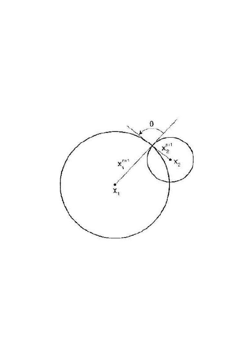
Figure 1: The spheres $x_{{}_{1}}^{{}^{\;\alpha}}$ and $x_{{}_{2}}^{{}^{\;\alpha}},$ $\alpha=1,2,\cdots$ $n,$ $n+1$, in $E^{{}^{n}}$ intersecting under angle $\theta$. Here the center $\mathbf{x}_{{}_{1}}$ stands for $\{x_{{}_{1}}^{\;1}$, $x_{{}_{1}}^{\;2}$, $\cdots$ $x_{{}_{1}}^{{}^{\;n}}\}$ and similarly for $\mathbf{x}_{{}_{2}}$.

To answer an expected immediate objection: of course $\mathbf{C}$’s transformations cannot act just on the 4-D space-time, with its length metric $ds^{2}=g_{\mu\nu}$ $dx^{{}^{\mu}}dx^{{}^{\nu}}$, because angle-preserving transformations of space-time do not in general preserve the length, and thus $\mathbf{C}$ would not be the symmetry group of this metric. (This was Einstein’s reason for rejecting the group $\mathbf{C}$, see [6].) The way to introduce the group $\mathbf{C}^{n}$ of conformal $(\equiv$ angle-preserving) transformations of $n$-dimensional euclidean space $E^{n}$ of coordinates $x^{{}^{\mu}},\mu=1,2\cdots n$, was well-known to the great geometers of the nineteenth century (F. Klein, Liouville, Möbius, Lie et al.) some 150 years ago, but seems unknown today, at least to modern theoretical physicists. In brief, one introduces the $(n+1)$–dimensional space of spheres in $E^{n}$ characterized by their centers $x^{{}^{\mu}}$ and radii $x^{n+1}$. The group $\mathbf{C}^{n}$ is then that group of transformations $x^{\prime^{\alpha}}=f^{{}^{\alpha}}(x^{1},x^{2},\cdots x^{n},x^{n+1}),$ $\alpha=1,2,\cdots n,n+1,$ which preserve the angle $\theta$ under which two spheres $x^{{}^{\alpha}}$ and $y^{{}^{\alpha}}$ intersect, see Fig. 1. For infinitesimally close spheres $y^{{}^{\alpha}}=x^{{}^{\alpha}}+dx^{{}^{\alpha}}$ one gets [7]

$$d\theta^{2}=(x^{n+1})^{-2}[(dx^{1})^{2}+(dx^{2})^{2}+\cdots(dx^{n})^{2}-(dx^{n+1})^{2}]\text{ .}$$ (5)

(This is nothing but the Law of Cosines, familiar from plane geometry class in high school.) The expression (5) defines the metric (dimensionless angle metric) of the appropriate $(n+1)$-dimensional Riemannian space which has the conformal group $\mathbf{C}^{n}$ as its symmetry group. It turns out that this space is not flat but is of constant curvature. All of this is explained in exhaustive detail elsewhere [7].

Thus for the pseudo-euclidean space-time with $n=4$ we get the 5-dimensional space with metric

$$d\theta^{2}=-\lambda^{-2}(d\mathbf{r}^{2}-dt^{2}+\sigma d\lambda^{2}),\sigma=\pm 1\text{ ,}$$ (6)

with $\{x^{1},x^{2},x^{3},x^{4}\}$ and $x^{5}$ renamed $\{x^{1},x^{2},x^{3},x^{0}\}$ and $\lambda$ respectively. Of course the “sphere” $x^{{}^{\alpha}}$ is the hyperboloid $g_{\mu\nu}(\xi^{{}^{\mu}}-x^{{}^{\mu}})(\xi^{{}^{\nu}}-x^{{}^{\nu}})+\sigma\lambda^{2}=0$ as a real locus. The sign $\sigma$, that is, whether the fifth dimension is spacelike $(\sigma=+)$ or timelike $(\sigma=-)$ is left open for the moment.

This concludes the informal, qualitative part of this Introduction.

We show here how the field equation for spin 1/2 fermions in five dimensions coupled to a self-force dependent on the fifth coordinate predicts point mass spectra of just a few points and non-uniform spacing. If the Casimir invariant of this particular irreducible unitary representation has a certain range, it is a 3-point spectrum for isospin up or down. The spectrum is consistent with the experimental bounds on the isospin-down quarks $d$, $s$, and $b$ for values of the coupling constant $\alpha$ of order unity and range $\kappa^{-1}$ of the spatial wave functions of a few fermis.

To avoid a possible confusion at the outset: this 5-D theory has nothing to do with the Kaluza or Kaluza-Klein theories. The enlargement of space-time to a five-dimensional manifold is forced, not arbitrary, if the conformal group is demanded as the basic kinematical symmetry group [7]. This fifth coordinate $\lambda$ is conjugate to mass just as position and time are conjugate to momentum and energy.  Partial derivatives with respect to $\lambda$ replace mass terms in fermion and boson field equations. In solutions of gauge boson field equations $\lambda$ plays the role of a microscopic length “parameter” which modifies the usual space-time causality of point particles. It gives point particles a structure or extension in a certain sense [7].

We argue in this paper that this five-dimensional extension of special relativity (“conformal relativity”) is the natural framework for a theory of elementary particle mass. The results obtained here are promising but are only a first step; the main problem is the exact form of the quantum-mechanical self-force. Some extra points, including a puzzle, are made in the concluding remarks. These also include an argument that the 5-D theory gives a theoretical basis for some features of the electroweak theory which were postulated on the basis of experiment alone.

2. SOME BACKGROUND

As explained in the Introduction, the metric of conformal relativity is [7]

$$d\theta^{2}=-\lambda^{-2}(dx^{2}+\sigma\text{ }d\lambda^{2})\text{ ,}$$

$$dx^{2}\equiv g_{\mu\nu}dx^{{}^{\mu}}dx^{\nu\text{ }},\qquad\mu,\nu=0,1,2,3;\text{ }x^{5}\equiv\lambda;\qquad\sigma=\pm\text{ ,}$$ (2.1)

where $d\theta$ is the infinitesimal angle under which spheres $(x^{{}^{\mu}},\lambda)$ and $(x^{{}^{\mu}}+dx^{{}^{\mu}},$ $\lambda+d\lambda)$ intersect. We use the metric $-g_{00}=g_{11}=g_{22}=g_{33}=+1$. Whether the extra dimension is spacelike $(\sigma=+)$ or timelike $(\sigma=-)$ is not yet clear, or maybe both occur. The ranges of the coordinates are $-\infty<x^{{}^{\mu}}<+\infty$ as usual, and $0<\lambda<\infty$ (or possibly $0<\mid\lambda\mid<\infty)$. The metric is singular if $\lambda=0$, so $\lambda=0$ is excluded from physical space, which is of course consistent with the action of the conformal group C [7]. We call these two 5-D Riemannian spaces (2.1) K₊ and K_- (after Felix Klein).

The field equation for spin 1/2 fermions in the C-covariant theory is [8]

$$(\gamma^{{}^{\alpha}}\nabla_{{}_{\alpha}}+\gamma\beta_{7}\nu)\text{ }\psi=0\text{ , }\qquad\nabla_{{}_{\alpha}}\equiv\stackrel{{\scriptstyle\gamma}}{{\nabla}}_{{}_{\alpha}}-ig\text{ }A_{{}_{\alpha}}\text{ .}$$ (2.2)

Here the six anticommuting $\gamma$-matrices obey

$$\gamma_{{}_{\alpha}}\gamma_{{}_{\beta}}+\gamma_{{}_{\beta}}\gamma_{{}_{\alpha}}=2\gamma_{\alpha\beta}\text{ }\mathbf{1}\text{, }\gamma_{{}_{\alpha}}\gamma+\gamma\gamma_{{}_{\alpha}}=0\text{, }\gamma^{2}=\mathbf{1}\text{ ,}$$ (2.3a)

$$\beta_{7}\equiv i\lambda^{5}\gamma_{1}\gamma_{2}\gamma_{3}\gamma_{0}\gamma_{5}\gamma\text{ ; }\alpha,\beta=0,1,2,3,5\text{ ,}$$ (2.3b)

where $\gamma_{\alpha\beta}$ is the angle metric (2.1). Indices are raised and lowered with this metric. $\stackrel{{\scriptstyle\gamma}}{{\nabla}}_{{}_{\alpha}}$ is the covariant derivative on spinors $\psi$ which fixes the spin algebra $\gamma_{{}_{\alpha}},\gamma$. (Note that the spaces $K_{{}_{\sigma}}$ are not flat, so that covariant derivatives occur in field equations.) We consider here only a $U(1)$ internal symmetry with gauge boson $A_{{}_{\alpha}}$. The equation (2.2) is uniquely fixed by requiring that the solutions $\psi$ span an irreducible unitary representation $(IUR)$ of C. The parameter $\nu$ is a Casimir invariant for this $IUR$, and Eq. (2.2) is the sole independent condition for spin 1/2 [8]. The six $\gamma_{{}_{\alpha}},\gamma$ are $8\times 8$ and $\psi$ is an 8-spinor because eight is the minimum dimension allowed for a matrix representation of the algebra (2.3a). When the spin connection is inserted, Eq. (2.2) reduces to

$$(\tilde{\gamma}\cdot D+\tilde{\gamma}^{5}D_{5}+2\sigma\lambda\tilde{\gamma}_{5}+\nu\beta_{7})\psi=0\text{ ,}$$

$$\tilde{\gamma}_{{}_{\alpha}}\equiv\gamma\gamma_{{}_{\alpha}}\text{ , }\qquad D_{{}_{\alpha}}\equiv\partial_{{}_{\alpha}}-igA_{{}_{\alpha}}\text{ ,}$$ (2.4)

where the ^∙ will always mean the 4-D scalar product $\tilde{\gamma}\cdot D\equiv\tilde{\gamma}^{{}^{\mu}}D_{{}_{\mu}}$. Note that $D_{{}_{\alpha}}$ involves the ordinary partial derivative $\partial_{{}_{\alpha}}$ ; the third term in Eq. (2.4) comes from the spin connection.

To be able to calculate with Eq. (2.4) a representation of the six $8\times 8$ matrices $\gamma_{{}_{\alpha}},\gamma$ must of course be chosen. We choose $\gamma_{{}_{\alpha}}=\gamma\stackrel{{\scriptstyle\sim}}{{\gamma_{{}_{\alpha}}}}$ and

$$\stackrel{{\scriptstyle\sim}}{{\gamma}}_{{}_{\mu}}=\lambda^{-1}\left(\begin{array}[]{ll}-\gamma_{{}_{\mu}}&0\\ 0&\gamma_{{}_{\mu}}\end{array}\right),\stackrel{{\scriptstyle\sim}}{{\gamma_{\text{ }}}}_{5}\text{ }=\lambda^{-1}\left(\begin{array}[]{ll}h&0\\ 0&-h\end{array}\right),\gamma=\left(\begin{array}[]{ll}0&1\\ 1&0\end{array}\right).$$ (2.5a)

The $\stackrel{{\scriptstyle\sim}}{{\gamma}}^{\text{ }\alpha}$are obtained by raising the indices with the metric (2.1). For the $4\times 4$ $\gamma_{{}_{\mu}},$ $h,$ and $1$ in these matrices, see Eq. (2.6). Then $\beta_{7}$, Eq. (2.3b), is

$$\beta_{7}=\left(\begin{array}[]{ll}1&0\\ 0&-1\end{array}\right)\text{ .}$$ (2.5b)

It can be shown (unpublished) that by comparing a Lagrangian for the spin 1/2 field equation (2.4) with the Lagrangian for the electroweak theory ([1], Chap. 7) that we can identify the upper and lower 4-spinors in the 8-spinor $\psi$ as the $T_{3}=+1/2$ and $-1/2$ components of the isodoublets of the electroweak theory in this representation. In fact, the whole electroweak theory can be reproduced. More on this in Sec. 4. Therefore we call the representation (2.5) the EW (electroweak) representation. The field equation (2.4) written in the $EW$ representation splits cleanly into wave equations for the $T_{3}=+1/2$ and $-1/2$ components (there is no coupling between these fields) and further, these wave equations are identical.

This common wave equation for the case $\sigma=-$ is

$$\{\gamma\cdot(\partial-ig\text{ }A)-ih(\partial_{5}-ig\text{ }A_{5})+(\nu+2ih)/\lambda\}\psi=0\text{ ,}$$

$$\gamma_{{}_{\mu}}\gamma_{{}_{\nu}}+\gamma_{{}_{\nu}}\gamma_{{}_{\mu}}=2g_{\mu\nu}\mathbf{1}\text{ , }h\equiv i\gamma_{1}\gamma_{2}\gamma_{3}\gamma_{0}\text{ .}$$ (2.6)

Here the $\gamma_{{}_{\mu}}$ are the usual $4\times 4$ constant $\gamma$-matrices, $\psi$ is now a $4$-spinor, and $h$ is the handedness operator (usually called $\gamma_{5}$ in the literature): $h\psi_{L}=-\psi_{L}$, $h\psi_{R}=+\psi_{R}$ for left and right-handed spinors.

The field equation for the gauge boson $A_{{}_{\alpha}}$ is

$$\stackrel{{\scriptstyle\gamma}}{{\nabla}}_{{}_{\alpha}}F_{\;\;{}_{\beta}}^{{}^{\alpha}}=0\text{ , }\qquad F_{\alpha\beta}\equiv\partial_{{}_{\alpha}}A_{{}_{\beta}}-\partial_{{}_{\beta}}A_{{}_{\alpha}\text{ }}\text{.}$$ (2.7)

These are reduced to a set of partial differential equations for the $5$-vector $A_{{}_{\alpha}}$ in Ref. [7].

3. FERMION MASS SPECTRUM FOR A TIMELIKE FIFTH DIMENSION

We look at stationary states: $\psi(t,\mathbf{r},\lambda)=e^{-iEt}g(\mathbf{r},\lambda)$ of Eq. (2.6). If we insert a self-force $A_{{}_{\alpha}}^{SF}$ and solve for a resting spin 1/2 fermion, the energy spectrum should be the mass spectrum: $E=M$. The self-force should certainly involve the fifth coordinate $\lambda$, so we adopt provisionally

$$A_{0}^{SF}=-g^{\prime}/\lambda\text{, other }A_{{}_{\alpha}}^{SF}\equiv 0\text{ .}$$ (3.1)

More on this in Sec. 4. Then the equation becomes

$$\left\{\gamma^{0}(M-\alpha/\lambda)+i\mathbf{\gamma}\cdot\mathbf{\partial}+h\partial_{{}_{\lambda}}+(i\nu-2h)/\lambda\right\}\text{ }g(\mathbf{r},\lambda)=0\text{. }$$ (3.2)

Here $\alpha\equiv g^{\prime}g$ ($g^{\prime}=g$ is natural for a self-force, but we leave this open for generality.) Consider $s$-states $g(r,\lambda)$ only; then $i\mathbf{\gamma}\cdot\mathbf{\partial}$ becomes $i\gamma_{r}\partial_{r}$ where $\gamma_{r}\equiv\mathbf{\gamma}\cdot\mathbf{n}$, $\mathbf{n}$ a unit 3-vector. We seek a separable solution in $r$ and $\lambda$, so take $g(r,\lambda)=e^{-\kappa r}g(\lambda)$ with $\kappa$ real and positive. Eq. (3.2) then reduces to the ordinary differential equation in $\lambda$

$$\left\{\gamma^{0}(M-\alpha/\lambda)-i\kappa\gamma_{r}+h\partial_{{}_{\lambda}}+(i\nu-2h)/\lambda\right\}g(\lambda)=0.$$ (3.3)

The solution is given in the Appendix. It is formally very similar to the solution of the Dirac equation for the relativistic hydrogen atom [9] with $\lambda$ and the mass levels of the particle playing the roles of $r$ and the hydrogenic energy levels, respectively. (The spectrum is very different however.) The mass spectrum is

$$M_{(n^{\prime},\tau)}/\kappa=\mid S_{{}_{\tau}}+n^{\prime}\mid\diagup[\alpha^{2}-(S_{{}_{\tau}}+n^{\prime})^{2}]^{1/2}$$

$$n^{\prime}=0,1,2,3,\cdot\cdot\cdot\text{ }\qquad,\text{ }\tau=\pm\text{ }\qquad,$$ (3.4a)

$$S_{{}_{\tau}}\equiv\tau(\alpha^{2}-\nu^{2})^{1/2}\text{ ,}$$ (3.4b)

$$S_{{}_{\tau}}+n^{\prime}\text{ has the sign of }\alpha\equiv g^{\prime}g\text{ ,}$$ (3.4c)

norm restriction:

$$(\alpha^{2}-\nu^{2})^{1/2}<1/2\text{ for }\tau=-\text{ .}$$ (3.4d)

One can see first in a general sort of way that this is a finite point spectrum: when the radicand in the denominator of Eq. (3.4a) goes negative, the spectrum ends. In fact, if we choose $\gamma\equiv(\alpha^{2}-\nu^{2})^{1/2}$ as a convenient independent variable (do not confuse this $\gamma$ with the matrix $\gamma$ in Eq. (2.3)!) and set $F(\gamma;n^{\prime},\tau)\equiv\alpha^{2}-(S_{{}_{\tau}}+n^{\prime})^{2}$, we get, on expanding and cancelling etc.

$$F(\gamma;n^{\prime},\tau)=-2n^{\prime}\tau\gamma+\nu^{2}-n^{\prime 2}\text{ .}$$ (3.5)

Now choose $g^{\prime}=g$, or $\alpha\equiv g^{2}>0,$ as seems natural. Then the necessary and sufficient conditions for a spectral point $(n^{\prime},\tau)$ are

$$\gamma<(\nu^{2}-n^{\prime 2})\diagup 2n^{\prime}\text{ , }\tau=+\text{ ; }\gamma>(n^{\prime 2}-\nu^{2})\diagup 2n^{\prime},\text{ }\tau=-\text{ , }$$ (3.6a)

$$\gamma<n^{\prime}\text{ for }\tau=-\text{ }\qquad,$$ (3.6b)

$$\gamma<1/2\text{ for }\tau=-\qquad.$$ (3.6c)

These are respectively from $F(\gamma;n^{\prime}\tau)>0$, Eq. (3.4c) for $\alpha>0$, and Eq. (3.4d).

In modern particle theory there are three families (isodoublets) of quarks and three of leptons. Relevant to this, the following theorem can be proved from the conditions (3.6a, b, c):

Theorem. There are three and only three mass levels if and only if $1<\nu^{2}<2$. These levels are $(n^{\prime},\tau)=(0,+)$, $(1,-)$, and $(1,+)$.

The mass spectrum written in terms of $\gamma$ is

$$M_{(n^{\prime},\tau)}\diagup\kappa=(\tau\gamma+n^{\prime})\diagup(-2n^{\prime}\tau\gamma-n^{\prime 2}+\nu^{2})^{1/2}$$ (3.7)

from just above. Thus for the three levels $(0,+)$, $(1,-)$, and $(1,+)$ we get

$$\begin{array}[]{lll}M_{(0,+)}\diagup\kappa&=&\gamma\diagup\mid\nu\mid\text{ ,}\\ &&\\ M_{(1,-)}\diagup\kappa&=&(1-\gamma)\diagup(2\gamma-1+\nu^{2})^{1/2}\text{ ,}\\ &&\\ M_{(1,+)}\diagup\kappa&=&(1+\gamma)\diagup(-2\gamma-1+\nu^{2})^{1/2}\text{ ,}\\ &&\\ 1<\nu^{2}<2&,&0<\gamma<1/2\text{ }\qquad.\end{array}$$ (3.8)

Then from these expressions one can deduce that the only possibility that one mass is much greater than the other two is

$$\nu^{2}=1+2\gamma+\varepsilon\text{ , }\qquad 0<\varepsilon<<1\text{ ,}$$ (3.9)

in which case $M_{(1,+)}$ is the large one. (This assumes $\varepsilon<<\gamma.$)

Fitting the quarks. We try to fit the $T_{3}=-1/2$ set of quarks $d$, $s$, and $b$. The experimental mass limits in $MeV$ are [10]

$$M_{d}=3-9\text{, }M_{s}=60-170\text{, }M_{b}=4100-4400.$$ (3.10)

So we adopt the value (3.9) for $\nu^{2}$ and identify $(1,+)\equiv b$. Next, inserting $\nu^{2}$ (3.9) into the mass formulae (3.8) and neglecting $\varepsilon$ in $(0,+)$ and $(1,-)$, we get the ratio

$$M_{(1,-)}\diagup M_{(0,+)}=(1-\gamma)(1+2\gamma)^{1/2}\diagup 2\gamma^{3/2}\text{ .}$$ (3.11)

It can be checked that this ratio is always $>1$ for $0<\gamma<1/2$, so we choose $(1,-)\equiv s$ and $(0,+)\equiv d$. Now equate the ratio (3.11) to $M_{s}/M_{d}$, using the average values $M_{d}=6$ $MeV$ and $M_{s}=115$ $MeV$. The resulting equation

$$(1-\gamma)(1+2\gamma)^{1/2}=38.4\text{ }\gamma^{3/2}$$ (3.12)

has the solution $\gamma\approx.088$. Finally, to determine $\varepsilon$, set the theoretical and experimental ratios $M_{b}/M_{d}$ equal. This gives

$$(1+\gamma)\mid\nu\mid\diagup\gamma\varepsilon^{1/2}=(M_{b}/M_{d})\text{ }_{\exp tl\text{ }}\text{.}$$ (3.13)

Insert $\gamma=.088$ and $\mid\nu\mid=1.088$ and use the minimum value $4100/9\approx 455$ for the ratio on the right to get the maximum size of $\varepsilon$. This gives $\varepsilon_{\max}\approx 8.7\times 10^{-4}$, and verifies our assumption $\varepsilon<<\gamma$.

The values of the coupling constant $\alpha$ and the range $\kappa^{-1}$ of the spatial wave functions are also of interest. We can evaluate $\kappa$ from $\kappa(M_{(n^{\prime},\tau)}/\kappa)=(M_{q})_{\exp tl}$. If we use the same average values for $M_{d}$ and $M_{s}$ as used above to determine $\gamma$, we will get the same $\kappa$ for either $(1,-)$ or $(0,+)$. Choose $(0,+).$

$$\kappa\gamma/\mid\nu\mid\text{ }=.081\kappa=6\text{ }MeV\Rightarrow\kappa=74.2\text{ }MeV\text{, }$$

which gives $\kappa^{-1}\approx 200/74.2\approx 2.7$ $f$. Also $\alpha^{2}=\gamma^{2}+\nu^{2}\approx 1.18$, or $\alpha\approx 1.09$, which suggests a self-force of QCD origin.

In summary, a fit to the three isospin-down quarks $d$, $s$, and $b$ has been obtained as the levels

$$(0,+)\equiv d\text{, }\qquad(1,-)\equiv s\text{ ,}\qquad(1,+)\equiv b$$ (3.14a)

for the Casimir invariant $\nu^{2}\approx 1.176$ and the reasonable values of the physical parameters

$$\alpha\approx 1.09\text{ and }\kappa^{-1}\approx 2.7\text{ }f\text{ .}$$ (3.14b)

Of course nearby values of these parameters will also give a fit owing to the wide latitude (3.10) in the experimental masses.

4. CONCLUDING REMARKS

A further characteristic of this theory necessary in any theory of mass should be mentioned. In inelastic scattering of elementary particles, energy and momentum are conserved but mass is not. Thus in any theory which unifies these quantities in some sense mass must be qualitatively different from energy and momentum and so must the conjugate quantities. Now note that the fifth coordinate $\lambda$ is qualitatively different from the other four $x^{{}^{\mu}}$; look for example at the metric (2.1). Further, the symmetry group C includes translation groups on $\mathbf{r\ }$and $t$, hence momentum and energy are conserved in particle scattering [11]. But there is no translation group on $\lambda$ [7], so the conjugate quantity mass need not be conserved.

The mass spectrum analyzed in Sec. 3 does fit the experimental numbers for the quarks, at least to within their (very loose) bounds. However, this spectrum is not intended to be final and quantitative at this stage. We only meant to show here that this particular 5-D theory required by conformal symmetry is capable of predicting few-point mass spectra of the right order of magnitude. The main problem is the crudity of the self-force (3.1) adopted. This field does not in fact satisfy the boson field equations (2.7) (see Ref. [7]) and must therefore be thought of as an approximation to an actual solution or simply as a model. A quantitative theory needs a realistic self-force, perhaps one involving also $SU(2)$ gauge bosons.

A few other points, including some puzzles, will be mentioned.

1)  The signature $\sigma=-$ was needed for an interesting mass spectrum. We can show that for $\sigma=+$ a one-point spectrum results for $\alpha>0$ (unpublished). The puzzle here is that $\sigma=+$ is definitely indicated in the classical self-force theory [7], which successfully resolves the anomalies due to classical point particles.

2)  Notice that if the lepton self-force is electromagnetic: $\alpha\approx 1/137,$ the mass spectrum (3.4) cannot fit the $T_{3}=-1/2$ leptons $e$, $\mu$, and $\tau$ since then $\gamma\equiv(\alpha^{2}-\nu^{2})^{1/2}$ is pure imaginary for $1<\nu^{2}<2$. This is a puzzle. But we add that for $\sigma=+,$ $(\nu^{2}-\alpha^{2})^{1/2}$ occurs where $(\alpha^{2}-\nu^{2})^{1/2}$ occurs for $\sigma=-$, hence the equation (3.2) written for $\sigma=+$ with a better self-force than (3.1) might work.

3)  For perfectly free spin 1/2 fermions (no external force and no self-force) the field equation (2.4) with $A_{{}_{\alpha}}\equiv 0$, $\sigma=+$ or $-$, space-time dependence in $e^{ip\cdot x}$ with $p^{2}+m^{2}=0$, and $\gamma_{{}_{\alpha}}$ and $\gamma$ in the EW representation is easily solved. The $\lambda$-dependence is in factors $\lambda^{5/2}Z_{\mu_{L}}(m\lambda)$ and $\lambda^{5/2}Z_{\mu_{R}}(m\lambda)$ for the $L$- and $R$-handed components of $\psi$, with $\mu_{L}\neq\mu_{R}$. The $Z_{{}_{\mu}}$ are cylinder functions of order $\mu$. The mass spectrum is continuous, $0\leq m<\infty$. In the case $\sigma=+$ if $\nu=-1/2$ is chosen for the Casimir invariant, then in the limit $m\rightarrow 0$ (neutrino solution) only a left-handed neutrino survives. This makes the value $\nu=-1/2$ very attractive theoretically for leptons. Perfectly free fermions are unphysical because of the continuous mass spectrum. But this also supports the idea that the mass problem for leptons should be phrased in the space $\sigma=+$ (cf. point (2) above) with $\nu=-1/2$.

4)  As indicated briefly above, this theory based on C instead of P as the kinematical symmetry group of particle physics is compatible with the EW theory. Further, it furnishes a theoretical foundation for some of the features of that theory adopted on the basis of experiment. Consider the following points. (a) The six basic anticommuting $\gamma$-matrices (2.3a) demand an 8-dimensional spinspace, thus allowing the upper and lower 4-spinors to be identified with the $T_{3}=\pm 1/2$ isodoublets. (b) But more than this, in the differential operator involving the primary gauge bosons B${}_{{}_{\alpha}}$ and W${}_{{}_{\alpha}}$ ⁱ
$(i=1,2,3)$, the spin algebra of the $SU(2)\times U(1)$ internal symmetry group is formed entirely from the $8\times 8$ $\gamma$-matrices (2.3a,b). Define the matrices

$$\tau_{i}\equiv\gamma\text{ , }\tau_{2}\equiv i\gamma\beta_{7}\text{ , }\tau_{3}\equiv\beta_{7}\text{ .}$$ (4.1)

Then these have the same commutation relations as the Pauli matrices. Further, in the EW representation (2.5) they take exactly the standard form, where the 1’s and 0’s are $4\times 4$. Contrast this with the situation in the present day EW theory where generators of the internal symmetry group $SU(2)$, unrelated to the $\gamma_{{}_{\mu}}$, are imported from the outside. The handedness projections $P_{h^{\prime}}$, $h^{\prime}=\pm$, are built from the $8\times 8$ $H\equiv\lambda\beta_{7}\widetilde{\gamma}_{5}$, which takes the form

$$H=\left(\begin{array}[]{ll}h&0\\ 0&h\end{array}\right)\text{ ,}$$ (4.2)

where $h$ is the $4\times 4$ handedness operator (see below Eq. (2.6)), in the EW representation. (c) If the Lagrangian

$$\mathcal{L}=\bar{\psi}\left[\tilde{\gamma}\cdot D+\tilde{\gamma}\text{ }^{5}\text{ }D_{5}+2\sigma\lambda\tilde{\gamma}_{5}+\nu\beta_{7}\right]\psi\text{ ,}$$ (4.3)

which yields the field equation (2.4), is equipped with the gauge bosons $B_{{}_{\alpha}}$ and $W_{{}_{\alpha}}$ ⁱ, it exactly reproduces the Lagrangian of the EW theory ([1], Chap. 7) plus some extra terms coming from the fifth components $B_{5}$ and $W_{5}$ ⁱ, presumably small corrections to the $4-D$ theory. Then the standard mixing produces the photon and $Z$ fields. d) However, the aspect in which this theory is not compatible with the EW theory (or the whole Standard Model) is the main point of this paper. In this theory the fermions may be massive, like the quarks considered in this paper. The fifth dimension plus an appropriate self force provides the masses. The Higgs mechanism is unnecessary.

APPENDIX. SOLUTION FOR THE MASS EIGENSTATES AND SPECTRUM

Insert the formally $2\times 2$ representation

$$\gamma^{0}=i\left(\begin{array}[]{ll}0&1\\ 1&0\end{array}\right)\text{, }\gamma_{r}=i\left(\begin{array}[]{ll}0&-1\\ 1&0\end{array}\right)\text{, }h=\left(\begin{array}[]{ll}1&0\\ 0&-1\end{array}\right)$$ (A1)

and $g(\lambda)=\left(\begin{array}[]{l}F\\ G\end{array}\right)$ into Eq. (3.3). $F$ and $G$ are thus 2-spinors; in fact $F=g_{R}$ and $G=g_{L}$ in view of the form (A1) of the handedness operator $h$. Multiplying by $-i$ we get

$$\begin{array}[]{l}(M-i\kappa-\alpha/\lambda)G-i(\partial_{{}_{\lambda}}+(i\nu-2)/\lambda)F=0\text{ ,}\\ \\ (M+i\kappa-\alpha/\lambda)F+i(\partial_{{}_{\lambda}}-(i\nu+2)/\lambda)G=0\text{ .}\end{array}$$ (A2)

Rephase: $iF\rightarrow F$, $G\rightarrow G$. Define

$$\beta_{1}\equiv M+i\kappa\text{, }\beta_{2}\equiv M-i\kappa\text{, }\beta^{2}\equiv\beta_{1}\beta_{2}=M^{2}+\kappa^{2}\text{.}$$ (A3)

Divide equations $(A2)$ by $\beta\equiv\sqrt{\beta^{2}}$ and put $\beta\lambda\equiv\tau$.

$$\begin{array}[]{l}(\beta_{2}/\beta-\alpha/\tau)G-(\partial_{{}_{\tau}}+(i\nu-2)/\tau)F=0\text{ ,}\\ \\ (\beta_{1}/\beta-\alpha/\tau)F-(\partial_{{}_{\tau}}-(i\nu+2)/\tau)G=0\text{ .}\end{array}$$ (A4)

Set $F,G\equiv e^{-\tau}(f,g)$. Then $\partial_{{}_{\tau}}F=(\dot{f}-f)e^{-\tau}$ etc. where ${}^{\bullet}\equiv\partial/\partial\tau$. Solve the equations in terms of $f$ and $g$  by the power series

$$f=\tau^{s}\sum\limits_{n=0}^{\infty}a_{n}\tau^{n}\text{ , }g=\tau^{s}\sum_{n=0}^{\infty}b_{n}\tau^{n}\text{, }a_{0}\text{ and }b_{0}\neq 0\text{ .}$$ (A5)

When these power series are inserted into the equations for $f$ and $g$ and coefficients of $\tau^{s+n-1}$ equated to $0$, we obtain

$$\begin{array}[]{l}(\beta_{2}/\beta)b_{n-1}-\alpha b_{n}-(s+n)a_{n}+a_{n-1}-(i\nu-2)a_{n}=0\text{ ,}\\ \\ (\beta_{1}/\beta)a_{n-1}-\alpha a_{n}-(s+n)b_{n}+b_{n-1}+(i\nu+2)b_{n}=0\text{ .}\end{array}$$ (A6)

Multiply the top equation (A6) by $\beta_{1}/\beta$ and subtract the bottom equation. The terms $a_{n-1}$ and $b_{n-1}$ go out since $\beta_{1}\beta_{2}/\beta^{2}=1$. After rearrangement this gives

$$\left[(\beta_{1}/\beta)(s+n-2+i\nu)-\alpha\right]a_{n}=\left[s+n-2-i\nu-\beta_{1}\alpha/\beta_{2}\right]b_{n}\text{.}$$ (A7)

To get the indicial equation choose $n=0$ in Eq. (A6) and ignore the terms $a_{-1}$ and $b_{-1}$. The determinant must vanish so that nonzero $a_{0}$ and $b_{0}$ result; the result is

$$S_{{}_{\eta}}\equiv s_{{}_{\eta}}-2=\eta(\alpha^{2}-\nu^{2})^{1/2}\text{, }\qquad\eta=\pm\text{ .}$$ (A8)

(We have changed the subscript $\tau$ on $S_{{}_{\tau}}$, Eq. (3.4b), to $\eta$ so as not to confuse it with the $\tau\equiv\beta\lambda$ of Eq. (A4) et seq.) This is Eq. (3.4b). By letting $n\rightarrow\infty$ in Eq. (A7) we get $b_{n}=(\beta_{1}/\beta)a_{n}$ in this limit; substituting this into both equations (A6) for $n\rightarrow\infty$, we find $a_{n}/a_{n-1}=2/n$ and the same for the $b$’$s$ in this limit. Thus both series (A5) diverge like $e^{2\tau}$, which is not allowed by the assumed finiteness of the norm. Hence both series must terminate:

$$a_{n^{\prime}+1}=b_{n^{\prime}+1}=0\text{ , }n^{\prime}=0,1,2,\cdots\text{ .}$$ (A9)

Set $n=n^{\prime}+1$ in Eq. (A6); we get $b_{n^{\prime}}=-(\beta_{1}/\beta)a_{n^{\prime}}$ . Put this result into Eq. (A7) for $n=n^{\prime}$. After cancellation of some terms and rearrangement

$$2(\beta_{1}/\beta)(s+n^{\prime}-2)-\alpha(1+(\beta_{1}/\beta)^{2})=0$$ (A10)

results. Divide this by $2\beta_{1}/\beta$ and use $\beta_{1}/\beta=\beta/\beta_{2}$. After some algebra we obtain

$$S_{{}_{\eta}}+n^{\prime}=\alpha M/\beta\text{ .}$$ (A11)

(This implies Eq. (3.4c).) Finally, do some algebra on Eq. (A11), using $\beta\equiv\sqrt{M^{2}+\kappa^{2}}$, to solve for $M$. This gives the mass spectrum (3.4a).

The mass eigenstates. From Sec. 3 and this Appendix, the mass eigenstates are $\psi=\left(\begin{array}[]{l}F\\ G\end{array}\right)$, where the $2$-spinors $F$ and $G$ are

$$F(t,r,\lambda)=e^{-iMt}\text{ }e^{-\kappa r}\text{ }F(\lambda)\text{ , \quad}G(t,r,\lambda)=e^{-iMt}\text{ }e^{-\kappa r}G(\lambda)\text{ ,}$$ (A12)

$$\begin{array}[]{l}F(\lambda)=(-i)e^{-\tau}\tau^{s_{{}_{\eta}}}\sum\limits_{n=0}^{n^{\prime}}a_{n}\tau^{n}\times u_{+}\text{ ,}\\ \\ G(\lambda)=e^{-\tau}\tau^{s_{{}_{\eta}}}\sum\limits_{n=0}^{n^{\prime}}b_{n}\tau^{n}\times u_{-}\text{ ,}\end{array}$$ (A13)

where

$$\tau\equiv\beta\lambda=\left[(M_{q}/\kappa)^{2}+1\right]^{1/2}\kappa\lambda\text{ .}$$ (A14)

Here the quantum number of the eigenstate $q\equiv(n^{\prime},\eta)$ and $M_{q}/\kappa$ is given by Eq. (3.4a) with the sign $\tau$ changed to $\eta$. The relation of the $b_{n}$ to $a_{n}$ and the $a_{n}$ to the $a_{n-1}$ are given by Eqs. (A7) and (A6). The constant $2$-spinors $u_{+}$ and $u_{-}$ are normalized in some way; the overall normalization of the $4$-spinor $\psi$ is secured by the free parameter $a_{0}$.

REFERENCES

[1] G. Kane, Modern Elementary Particle Physics (Addison-Wesley, New York, 1993), Chap. 8.

[2] P.C.W. Davies and J. Brown, Superstrings, a Theory of Everything? (Cambridge University Press, Cambridge, 1988).

[3] B. Greene, The Elegant Universe (Norton, New York, 1999).

[4] V. Bargmann and E.P. Wigner, Proc. Nat. Acad. Sci. 34, 211 (1948).

[5] F. Klein, Math. Ann. 5, 257 (1872). _______, Vorlesungen über Höhere Geometrie 3 Aufl, (Springer, Berlin 1926).

[6] A. Einstein, The Meaning of Relativity, 4th ed. (Princeton University Press, Princeton 1953).

[7] R. L. Ingraham, Int. J. Mod. Phys. 7, 603 (1998).

[8) R. L. Ingraham, Nuovo Cimento 68B, 203, 218 (1982).

[9] L.I. Schiff, Quantum Mechanics, 2nd ed. (McGraw-Hill, New York 1955), Sec. 44.

[10] Review of Particle Physics, Euro. Phys. J. C3 (1998), p. 24.

[11] J.M. Jauch and F. Rohrlich, The Theory of Photons and Electrons (Addison-Wesley, Cambridge U.S.A. 1955), Sec. 1-11.