Abstract

We develop some basic properties of the open string on the symmetric product which is supposed to describe the open string field theory in discrete lightcone quantization (DLCQ). After preparing the consistency conditions of the twisted boundary conditions for Annulus/Möbius/Klein Bottle amplitudes in generic non-abelian orbifold, we classify the most general solutions of the constraints when the discrete group is $S_{N}$. We calculate the corresponding orbifold amplitudes from two viewpoints – from the boundary state formalism and from the trace over the open string Hilbert space. It is shown that the topology of the world sheet for the short string and that of the long string in general do not coincide. For example the annulus sector for the short string contains all the sectors (torus, annulus, Klein bottle, Möbius strip) of the long strings. The boundary/cross-cap states of the short strings are classified into three categories in terms of the long string, the ordinary boundary and the cross-cap states, and the “joint” state which describes the connection of two short strings. We show that the sum of the all possible boundary conditions is equal to the exponential of the sum of the irreducible amplitude – one body amplitude of long open (closed) strings. This is typical structure of DLCQ partition function. We examined that the tadpole cancellation condition in our language and derived the well-known gauge group $SO(2^{13})$.

hep-th/0005111

1 Introduction

String field theory [1]–[8] has been one of the most fundamental and the most mysterious subjects in string theory. In the course of the development, it has been clarifying the gauge interactions among higher excited states [4][5], the moduli problem at least for the open string [4]. Originally it was regarded as the only candidate to describe the non-perturbative aspects of string theory.

The revolutionary developments in these years, however, the new ideas such as D-brane or M-theory turned out to play more fundamental rôle. One of the shortcoming of string field theory may be that it does not has direct means to describe D-branes dynamics although there were some attempts [9]. In this respect, people pay more interests in the alternative approaches such as the matrix models [10]–[12] where D-brane itself becomes the dynamical variable.

Some years ago, a novel approach [13]–[16] to string field theory was evolved from the matrix model view point. In the infrared, the theory is described as a conformal field theory on the symmetric product $S^{n}M=M^{\otimes n}/S_{n}$. The orbifold singularities of the target are described as the twisted sectors. Excitations belonging to each twisted sectors can be physically interpreted as the collections of the “long strings” which are composite of the fundamental string variable (“short string” or “string bit”). The theory therefore contains a mechanism of the splitting/joining interactions of the closed string naturally in its definition. The partition function is expressed as the exponential of the one body partition function of the long string [17]. This is typical structure of the partition function of the quantum field theory in the discrete lightcone quantization (DLCQ) [18] which is not restricted to the string theory. This is the analog of the fact that the vacuum amplitude can be expressed as the exponential of the contributions from the connected Feynmann diagrams in the conventional quantum field theories. These facts support the idea that the matrix string theory describes the string field theory in DLCQ.

In this direction, a steady progress was made. For example, the four point amplitudes of the string theory was directly calculated [21][22] by this method to reproduce Virasoro amplitude. It is applied to describe the little string theory [19][20] to reproduce the black-hole entropy formula. It was generalized to heterotic matrix strings [23]–[25] to describe the second quantized lightcone heterotic string. Some aspects of the $S_{N}$ orbifold CFT such as the modular properties and the fusion rule coefficients are studied in [26]. A lot of the developments are made in the context of the moduli space. In particular, the instanton sectors of two dimensional Yang-Mills theory is related to the nontrivial topology of the matrix string world sheet [29]–[33].

From the mathematical viewpoint, it is originated from the calculation of the elliptic genera [17][27] and has a direct relation with Götsche’s formula for Hilbert scheme of points [28] and generalized Kac-Moody algebras.

In this paper, we study the open string version of the matrix string theory. The motivation of this subject should be obvious since we can not escape from dealing with D-branes in the matrix strings. We use the explicit calculation based on the boundary conformal field theory on the orbifold [38]–[51] and give the some of the explicit analysis which should be made in BCFT. The new material is the appearance of the long open (closed) strings in the twisted sector of the open string. We give the classification theorem of all the possible form of such twisted sectors. We calculate the partition function for each twisted boundary conditions and show that it can be reducible to the amplitude of the one long string. An interesting feature is the world sheet topology of the short string is in general different from that of the long string. We develop also the boundary state formalism and reproduced the amplitude. If we sum up all possible boundary conditions, the partition function can be written as the exponential of the sum of the long string partition functions. This is the typical form of the partition function in the discrete lightcone gauge. Finally we confirmed that the dilaton tadpole cancellation occurs when the gauge group is famous $SO(2^{13})$ for the bosonic string.

Let us explain the organization of this paper. We put the main claims at the beginning of each section. One may first read these parts and skip the detailed explanation or the proof until it becomes necessary.

In section 2, we give a review of the basic structure of the orbifold theory on the symmetric product. We describe it in detail since some of the explicit calculations become essential later. We emphasize the aspect that it can be formulated as the conventional non-abelian orbifold theory. Namely for the torus amplitude, the consistency conditions for the twisted boundary condition contain all the information necessary to reproduce its characteristic feature of the string field theory. We also give a review of the discrete lightcone gauge and derived the typical form of its partition function.

In section 3, we investigate the constraint on the twisted boundary conditions for annulus/Möbius strip/Klein bottle amplitudes and relate it to the various boundary/cross-cap states [38]–[43]. Open string twisted sectors were discussed in literature [44]–[47] mainly for the abelian case. For non-abelian case, we need some extra care because of the non-commutativity. Because the open string twisted sector is the main object in this paper, we describe it in detail. The content of this section is generic and can be applied to arbitrary non-abelian orbifold models.

In section 4, we exactly solve the constraints for the symmetric product orbifold. The solution for the Klein bottle amplitude is similar to the torus case. In the Annulus and Möbius strip cases, there are some extra series of the solutions which will be interpreted as the contributions of the closed string sector. The content of this section is mathematical but is one of our main claim in this article.

In section 5, we calculate the one loop amplitude in two ways. First we do it by using the explicit operator formalism for the flat background. The calculation itself is technically similar to that of section 2. Second we calculate it by using multiple cover of the world sheet. The abstract combinatorial solutions in section 4 are translated into the form of the physically clear interpretation as the long string amplitudes. One interesting feature is the appearance of four sectors for the long string in each of the annulus and Möbius string amplitude for the short string. Namely, the topology of the world sheet seen from the long string is in general different from that for the short string as we already mentioned.

In section 6, we give the explicit form of the boundary/cross-cap states for the arbitrary twisted sectors. We argue that the boundary state for the short string can be classified into three types. The first one is the conventional boundary state for the long string. The second one turns out to be the cross-cap state for the long string. This is one of the origin of the topology change. The third one describes the connection of the two short strings. It encodes the nature of the string field theory of the orbifold theory. The cross-cap states for the short string have the similar classification. We calculate the inner product between them in order to examine the “modular invariance” or the tadpole condition in the next section.

In section 7, we first prove that each of three open string sectors can be expressed as the exponential of the one-body amplitudes of the long strings of the various scale. This is quite natural as the DLCQ partition function. The annulus amplitude for the short string contains all types of the amplitudes for the long string. One interesting aspect is that the torus amplitude which is contained there has the complex (but discrete) moduli parameter while the original annulus has only imaginary part.

In section 8, we examine the tadpole cancellation of the bosonic string in our context. We use only the annulus amplitude (for short string) to derive the tadpole condition. In this case there are cancellations among the massless parts of the boundary states (of the short string) alone. Since one-string partition function is exponentiated, one may reduce the tadpole condition to each one body problem for the long string. In this form, one can immediately reproduce the famous relation such as $SO(2^{13})$.

2 Review of closed string on symmetric product

2.1 Orbifold CFT on symmetric product

Let ${\bf X}^{I}(\tau,\sigma)$ (${\bf X}^{I}\in M$, $I=1,\cdots,N$) be the bosonic coordinates which define the string embedding on symmetric product $S^{N}M$. The twisted sectors ${\cal H}_{h}$ ($h\in S_{N}$) are defined by the boundary condition of ${\bf X}$,

$${\bf X}(\sigma_{0},\sigma_{1}+2\pi)=h\cdot{\bf X}(\sigma_{0},\sigma_{1}),$$ (2.1)

where $(h\cdot{\bf X})^{I}\equiv\sum_{J}h^{IJ}{\bf X}^{J}$.

The modular invariant partition function on torus is,

$$Z_{N}(\tau,\bar{\tau}) = \frac{1}{|S_{N}|}\sum_{{\scriptsize\begin{array}[]{c}g,h\in S_{N}\\ gh=hg\end{array}}}\chi_{h,g}(\tau,\bar{\tau})$$ (2.4)

$$\chi_{h,g}(\tau,\bar{\tau}) = \mbox{Tr}_{{\cal H}_{h}}(g\cdot{\bf e}\!\left[\tau L_{0}-\bar{\tau}\bar{L_{0}}\right]),$$ (2.5)

$${\bf e}\!\left[x\right] \equiv e^{2\pi ix}.$$ (2.6)

The summation in $g\in S_{N}$ is needed to define a projection onto the $S_{N}$ invariant subspace. The constraint

$$g\cdot h=h\cdot g$$ (2.7)

in (2.4) is the consistency condition of the path integral to assure that the twists in time and space directions commute.

In the non-abelian orbifold, only the conjugacy class of $h$ has the invariant meaning since $g\cdot{\bf X}\in{\cal H}_{ghg^{-1}}$ if ${\bf X}\in{\cal H}_{h}$. The summation in (2.4) over $h$ is then replaced by the summation over the conjugacy class ${\cal C}_{i}$ of $S_{N}$. For a particular element $h\in{\cal C}_{i}$, the solutions of (2.7) are the elements of the centralizer group ${\cal N}_{i}$. With the relation $|S_{N}|=|{\cal C}_{i}||{\cal N}_{i}|$, (2.7) can be rewritten as,

$$Z_{N}(\tau,\bar{\tau})=\sum_{i}\frac{1}{|{\cal N}_{i}|}\sum_{g\in{\cal N}_{i}}\chi_{h,g}(\tau,\bar{\tau}),\qquad h\in{\cal C}_{i}$$ (2.8)

This formula is the generic expression for the arbitrary non-abelian orbifold.

For the permutation group $S_{N}$, the conjugacy group is labeled by the partition of $N$, since any group element can be written as a product of elementary cycles $(n)$ of length $n$,

$$[h]=(1)^{N_{1}}(2)^{N_{2}}\cdots(k)^{N_{k}},\quad\sum_{n>0}nN_{n}=N.$$ (2.9)

The centralizer of such an element is a semi-direct product of factors $S_{N_{n}}$ and ${\bf Z}_{n}$,

$$g\in{\cal N}_{h}=S_{N_{1}}\times(S_{N_{2}}\ltimes{\bf Z}_{2}^{N_{2}})\times\cdots(S_{N_{k}}\ltimes{\bf Z}_{k}^{N_{k}}).$$ (2.10)

The factors $S_{N_{n}}$ permute the $N_{n}$ cycles $(n)$, while the factors ${\bf Z}_{n}$ rotate each cycle $(n)$. The order of the centralizer group is,

$$|{\cal N}_{h}|=\sum_{n=1}^{k}n^{N_{n}}\ N_{n}!$$ (2.11)

The physical interpretation of these factors are well-known. Let us first consider the case where $h$ is the element of the cyclic permutation of $N$ elements,

$$h={\cal T}_{N}:\quad{\bf X}^{I}\rightarrow{\bf X}^{I+1},\quad I\in\left\{0,1,\ldots,N-1\right\}.$$ (2.12)

Here superscript $I$ is defined by mod $N$. The twist by $h$ then gives the boundary condition,

$${\bf X}^{I}(\sigma_{0},\sigma_{1}+2\pi)={\bf X}^{I+1}(\sigma_{0},\sigma_{1}).$$ (2.13)

It means that $N$ short closed strings ${\bf X}^{I}$ are connected with each other to form one long string of length $n$. For the general situation (2.9), we will have $N_{n}$ long strings of length $n$ for $n=1,\ldots,k$. The short strings that form a long string are sometimes called “string bits”.

In this language, the element of the centralizer group (2.10) has a clear interpretation. ${\bf Z}_{n}$ factors are the rotations of the string bits that constitute a long string of length $n$. $S_{N_{n}}$ then reshuffle the long strings of the same length $n$ as a whole (figure 1).

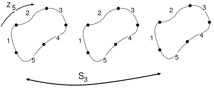
Figure 1: Long strings and the action of the centralizer group

2.2 Partition function

The long string interpretation can be established further by the calculation of the partition function. In this subsection, we would like to give somewhat more explicit computation compared with the literature for the preparation for later sections. To make our argument clear, we first restrict the situation where target space is flat $M={\bf R}^{1}$. We will then give a generic argument for the arbitrary target space.

2.2.1 Irreducible Diagram

In the calculation of the partition function (2.8), we need to divide $N$ free fields into small subgroups. Each subgroup consists of the collection of free fields which are mixed up by the action of two twists $h$ and $g$. It is obvious that there are minimal sets of free field which can not divided into subgroups. We call such a set of free fields as “irreducible set”. The partition function $\chi_{h,g}$ is identified as the product of the contributions of each irreducible sets.

In the torus case, it is known that such irreducible sets can be always reduced to $nm$ free fields where $h$ and $g$ act as,

$$h = diag({\cal T}_{n},\cdots,{\cal T}_{n})$$

$$g = diag({\cal T}_{n}^{p_{1}},\cdots,{\cal T}_{n}^{p_{m}})\cdot{\overline{\cal T}}_{m}\,\,,$$ (2.14)

where ${\overline{\cal T}}_{m}$ acts on ${\bf X}^{I,J}$ as $({\overline{\cal T}}_{m}\cdot{\bf X})^{I,J}={\bf X}^{I,J+1}$ and ${\cal T}_{n}$ acts as $({\cal T}_{n}\cdot{\bf X})^{I,J}={\bf X}^{I+1,J}$. We label $nm$ free fields as ${\bf X}^{I,J}$ ($I\in(0,1,\cdots,n-1)$ and $J\in(0,1,\cdots,m-1)$). $I$ (resp. $J$) is defined modulo $n$ (resp. $m$). $p_{J}$’s represent the rotations each long strings and take their values in $0,1,\cdots,n-1$.

The action of $h$ and $g$ on ${\bf X}$ in the component is given as,

$$(h\cdot{\bf X})^{I,J} = {\bf X}^{I+1,J}$$

$$(g\cdot{\bf X})^{I,J} = {\bf X}^{I+p_{J},J+1}$$ (2.15)

To make $h$ action diagonal, we introduce the discrete Fourier transformation with respect to $I$,

$$\widetilde{{\bf X}}^{a,J}\equiv\frac{1}{\sqrt{n}}\sum_{I=0}^{n-1}{\bf e}\!\left[-\frac{aI}{n}\right]{\bf X}^{I,J},\quad a\in(0,1,\cdots,n-1)$$ (2.16)

In this basis, the actions of $h,g$ are modified to,

$$(h\cdot\widetilde{\bf X})^{a,J} = {\bf e}\!\left[\frac{a}{n}\right]\widetilde{\bf X}^{a,J}$$

$$(g\cdot\widetilde{\bf X})^{a,J} = {\bf e}\!\left[\frac{ap_{J}}{n}\right]\widetilde{\bf X}^{a,J+1}$$ (2.17)

Since $h$ action is diagonalized, the periodicity of $\widetilde{\bf X}$ becomes well-defined,

$$\widetilde{\bf X}^{a,J}(\sigma_{0},\sigma_{1}+2\pi)={\bf e}\!\left[\frac{a}{n}\right]\widetilde{\bf X}^{a,J}(\sigma_{0},\sigma_{1}).$$ (2.18)

We have the mode expansion of $\widetilde{\bf X}^{a,J}$ as ($z=e^{i(\sigma_{1}+i\sigma_{0})}$),

$$\widetilde{\bf X}^{a,J}=\alpha_{0}^{J}\delta_{a,0}\sigma_{0}+i\sum_{r\in{\bf Z}}\left(\frac{1}{r-a/n}\alpha^{a,J}_{r-a/n}z^{-r+a/n}+\frac{1}{r+a/n}\tilde{\alpha}^{a,J}_{r+a/n}\bar{z}^{-r-a/n}\right)$$ (2.19)

with the commutation relation,

$$\left[\alpha^{a,I}_{r-a/n},\alpha^{b,J}_{s-b/n}\right]=(r-a/n)\delta_{I,J}\delta_{r+s}\delta_{a+b}\,\,.$$ (2.20)

In order to diagonalize $g$ action, we combine the oscillators further as,

$${\bf Y}^{a}\equiv\sum_{J=0}^{m-1}C_{J}\widetilde{\bf X}^{a,J}.$$ (2.21)

Eigenstate equation $g\cdot{\bf Y}^{a}=\mu{\bf Y}^{a}$ gives a relation between the neighboring coefficients,

$$\mu C_{J+1}={\bf e}\!\left[\frac{ap_{J}}{n}\right]C_{J}.$$ (2.22)

The periodicity condition $C_{m}=C_{0}$ implies,

$$\mu^{m}={\bf e}\!\left[\frac{ap}{n}\right],\quad p\equiv\sum_{J}p_{J}$$ (2.23)

The eigenvalues for $g$ action are evaluated as,

$$\mu^{a,b}={\bf e}\!\left[\frac{b}{m}+\frac{ap}{nm}\right],\quad a=0,1,\cdots,n-1,\quad b=0,1,\cdots,m-1.$$ (2.24)

In other word, the action of $g$ is diagonalized as

$$(g\,\alpha_{r-a/n})^{a,b}=\mu^{a,b}\alpha_{r-a/n}^{a,b},$$ (2.25)

where $\alpha^{a,b}$ are the linear combinations of $\alpha^{a,J}$.

The (chiral) oscillator part of the partition function can be now evaluated by using mode expansion and eigenvalues of $g$,

$$\prod_{r=1}^{\infty}\prod_{a=0}^{n-1}\prod_{b=0}^{m-1}\left(1-{\bf e}\!\left[\frac{b}{m}+\frac{ap}{nm}\right]{\bf e}\!\left[(r-a/n)\tau\right]\right)^{-1}$$

$$=\prod_{r=1}^{\infty}\prod_{a=0}^{n-1}\left(1-{\bf e}\!\left[\frac{ap}{n}\right]{\bf e}\!\left[m\tau(r-a/n)\right]\right)^{-1}$$

$$=\prod_{r=1}^{\infty}\prod_{a=0}^{n-1}\left(1-{\bf e}\!\left[-p(r-\frac{a}{n})\right]{\bf e}\!\left[m\tau(r-a/n)\right]\right)^{-1}$$

$$=\prod_{r=1}^{\infty}\left(1-{\bf e}\!\left[\left(\frac{m\tau-p}{n}\right)r\right]\right)^{-1}$$ (2.26)

Thus at least the chiral part of the partition function from $nm$ string bits are knitted together to give the partition function of one long string with modified moduli parameter

$$\frac{m\tau-p}{n}\equiv\tau_{n,m,p}\,\,.$$ (2.27)

As for the momentum integration, only the $a=0$ component have zero mode. In the remaining $m$ momentum, only $b=0$ part gives non-trivial inner product when $g$ is inserted. We conclude that zero-mode contribution comes from integration of single momentum. One subtlety is how to fix the normalization constant. While changing the variable from the short string to the long one, Virasoro generators should be modified to $L_{0}\rightarrow L_{0}/n$ [15]. Next since we have $m$ of such long strings moving coherently, we have to multiply it $m$. The kinetic term is thus modified to $\frac{mp^{2}}{2n}$. By integrating out $p$, we get

$$1/\sqrt{\mbox{Im}(\tau_{n,m,p})}\,\,.$$ (2.28)

By combining the contributions from the anti-chiral part and momentum integration, the partition function of $nm$ free fields becomes

$$Z(n,m,\left\{p\right\}|\tau,\bar{\tau})=Z_{1}\left(\tau_{n,m,p},\bar{\tau}_{n,m,p}\right)\,\,.$$ (2.29)

$Z_{1}(\tau,\bar{\tau})$ is the standard partition function for one free boson,

$$Z_{1}(\tau,\bar{\tau})=\frac{1}{\sqrt{\mbox{Im}\tau}}(\eta(\tau)\bar{\eta}(\bar{\tau}))^{-1}.$$ (2.30)

As we see in the next paragraph, (2.29) is the generic feature of the symmetric space orbifold. It may be physically interpreted as a kind of the renormalization. Namely path integral over the short string variables are replaced by that of the long string. The two formula coincides if we replace the moduli parameter.

2.2.2 Generalization of the target space

Our consideration in the previous subsection essentially depends on the flatness of the target space. We first review the general arguments on the arbitrary target space by using the path integral method.

Let $M$ be a general manifold where a string can live and consider the path integral on ${\bf X}^{I,J}\in M$ which satisfies

$${\bf X}^{I,J}(w+1)={\bf X}^{I+1,J}(w)\,\,,\qquad{\bf X}^{I,J}(w+\tau)={\bf X}^{I+p_{J},J+1}(w)\,\,,$$ (2.31)

for each irreducible set $h,g$ as in the previous subsection. Here ${\bf X}$ is defined on a small parallelogram with period $(1,\tau)$.

These fields ${\bf X}(w)$ can be rewritten from one field ${\cal X}(w)\in M$ by the identification,

$${\bf X}^{I,J}(w)={\cal X}\left(w+J\tau+I-P_{J}\right)\,\,,\quad P_{J}=\sum_{\ell=0}^{J-1}p_{\ell}\,\,.$$ (2.32)

${\cal X}$ has the following periodicity derived from ${\bf X}^{I+n,J}={\bf X}^{I,J+m}={\bf X}^{I,J}$,

$${\cal X}(w+n)={\cal X}(w)\,\,,\qquad{\cal X}(w+m\tau-p)={\cal X}(w)\,\,.$$ (2.33)

Namely, ${\cal X}(w)$ is defined on $nm$ combinations of the parallelogram with period $(n,m\tau-p)$. The moduli of the bigger torus is given by $\tau_{n,m,p}$.

Path integral over variable ${\bf X}$ should be the same as that of ${\cal X}$. It implies the generic rule for the arbitrary target space,

$$Z_{h,g}^{{\bf X}}(\tau,\bar{\tau})=Z^{{\cal X}}(\tau_{n,m,p},\bar{\tau}_{n,m,p}).$$ (2.34)

This type of the proof may look too abstract. One may give more concrete reasoning when the target space is the orbifold $M=T/\Gamma$ where $T$ is a flat space and $\Gamma$ is a discrete group which may be non-abelian. The total target space becomes $T^{N}/S_{N}\ltimes\Gamma^{N}$. The partition function is written as

$$Z_{N}=\frac{1}{|S_{N}|\cdot|\Gamma|^{N}}\sum_{\scriptsize\begin{array}[]{c}h,g\in S_{N}\\ hg=gh\end{array}}\sum_{\scriptsize\begin{array}[]{c}\left\{\alpha\right\},\left\{\beta\right\}\in\Gamma\\ \left\{\alpha\right\}\cdot\left\{\beta\right\}^{h}=\left\{\beta\right\}\cdot\left\{\alpha\right\}^{g}\end{array}}\,\,\mbox{Tr}_{{\cal H}_{h,\left\{\alpha\right\}}}\left(g\,\beta\,q^{L_{0}}\bar{q}^{\bar{L}_{0}}\right).$$ (2.35)

Here $\left\{\alpha\right\},\left\{\beta\right\}$ define the boundary condition for ${\bf X}$ for fixed $h,g\in S_{N}$ as,

$${\bf X}^{i}(w+1)=\alpha^{i}\cdot{\bf X}^{h(i)}(w)\,\,,\qquad{\bf X}^{i}(w+\tau)=\beta^{i}\cdot{\bf X}^{g(i)}(w)\,\,.$$ (2.36)

The condition $\left\{\alpha\right\}\cdot\left\{\beta\right\}^{h}=\left\{\beta\right\}\cdot\left\{\alpha\right\}^{g}$ in the summation signifies the “integrability condition” of these boundary conditions,

$$\alpha^{i}\beta^{h(i)}=\beta^{i}\alpha^{g(i)}\,\,,\qquad i=1,2,\cdots,N\,\,.$$ (2.37)

For irreducible variables with $h,g$ given as (2.2.1), we replace the index $i$ to a pair $I,J$ and rewrite the boundary conditions and consistency conditions

$${\bf X}^{I,J}(w+1)=\alpha^{I,J}\cdot{\bf X}^{I+1,J}(w)\,\,,\qquad{\bf X}^{I,J}(w+\tau)=\beta^{I,J}\cdot{\bf X}^{I+p_{J},J+1}(w)\,\,,$$

$$\beta^{I,J}\cdot\alpha^{I+p_{J},J+1}=\alpha^{I,J}\cdot\beta^{I+1,J}.$$ (2.38)

With this type of the constraint, one can always find a unique set $\gamma^{I,J}\in\Gamma$ which satisfies,

$$\gamma^{0,0}=1\,,\quad\alpha^{I,J}=\gamma^{I,J}(\gamma^{I+1,J})^{-1}\,,\quad\beta^{I,J}=\gamma^{I,J}(\gamma^{I+p_{J},J+1})^{-1}\,.$$ (2.39)

With this twist factor, one may introduce ${\cal X}(w)\in T$ as before which is defined on the bigger torus generated by $(n,m\tau-p)$ and relate it ${\bf X}^{IJ}$ as

$${\bf X}^{I,J}(w)=\gamma^{IJ}{\cal X}(w+J\tau+I-P_{J})\,\,.$$ (2.40)

It is easy to derive that ${\bf X}$ thus defined satisfies (2.38). In terms of ${\cal X}$ one may develop the operator formalism as before. Since $\gamma$ factors are just redefinition of the identification between the variables, The partition function with different $\gamma$ will produce identical partition function. It will give a factor $|\Gamma|^{nm-1}$. The only nontrivial element is the global monodromy factor $A,B\in\Gamma$ defined by,

$$A=\gamma^{n,0},\quad B=\gamma^{0,m}\,\,,$$ (2.41)

which defines the boundary condition for $\chi(w)$,

$${\cal X}(w+n)=A^{-1}\,{\cal X}(w)\,,\quad{\cal X}(w+m\tau-p)=B^{-1}\,{\cal X}(w)\,.$$ (2.42)

We thus arrive at the desired relation,

$$\frac{1}{|\Gamma|^{nm}}\sum_{\scriptsize\begin{array}[]{c}\left\{\alpha\right\},\left\{\beta\right\}\in\Gamma\\ \left\{\alpha\right\}\cdot\left\{\beta\right\}^{h}=\left\{\beta\right\}\cdot\left\{\alpha\right\}^{g}\end{array}}\,\,Z^{{\bf X}}_{h,\left\{\alpha\right\},g,\left\{\beta\right\}}(\tau,\bar{\tau})=\frac{1}{|\Gamma|}\sum_{\scriptsize\begin{array}[]{c}A,B\in\Gamma\\ AB=BA\end{array}}\,Z^{{\cal X}}_{A,B}(\tau_{n,m,p},\bar{\tau}_{n,m,p}).$$ (2.43)

The partition function for ${\cal X}$ can be obtained by the explicit operator formalism and obviously identical to the single string partition function. One may conclude that the formula (2.29) should hold for any target space by replacing $Z_{1}$ by the partition function of the single string in that target space.

2.2.3 Generating function of the partition function

In order to evaluate the whole partition function (2.4), we need to follow some steps.

1. As we mentioned in the previous subsection, $\chi_{h,g}$ in (2.4) is expressed as the product of the contributions from the irreducible sets (2.29). We need to specify how many of such irreducible sets are contained in given pair $h,g$.

2. As for $h$, we use the representation of the conjugacy class (2.9) and use the definition (2.8).

3. For each $h$, $g$ is an element of the centralizer group (2.10). If we restrict the sector $h={\cal T}_{n}^{\otimes N_{n}}$, $g$ can be written as $S_{N_{n}}\ltimes{\bf Z}_{n}^{N_{n}}$. Elements in $S_{N_{n}}$ should be again decomposed into conjugacy class as $(1)^{M_{n,1}}(2)^{M_{n,2}}(3)^{M_{n,3}}\ldots$ with the constraint,

   $$\sum_{s_{n}=1}^{\infty}s_{n}M_{n,s_{n}}=N_{n}.$$ (2.44)

4. In this decomposition, we have $M_{n,m}$ irreducible subsets for each $n,m$. By summation over elements in ${\bf Z}_{n}$ (namely $p_{\ell}$ in (2.2.1)), we get the expression of $\chi_{h,g}$,

   $$\chi_{h,g} = \prod_{n,m=1}^{\infty}(n^{m}Z(n,m))^{M_{n,m}}$$ (2.45)

   $$Z(n,m) = \frac{1}{n^{m}}\sum_{\left\{p\right\}}Z(n,m,\left\{p\right\}|\tau,\bar{\tau})=\frac{1}{n}\sum_{p}Z(n,m,p|\tau,\bar{\tau}).$$ (2.46)

   We used the fact that the partition function (2.29) depends only on the sum of $\left\{p\right\}$.

5. For each, $(\left\{N\right\},\left\{M\right\})$, the weight factor is

   $$\frac{1}{\prod_{n=1}^{\infty}n^{N_{n}}N_{n}!}\prod_{n=1}^{\infty}\left(\frac{N_{n}!}{\prod_{s_{n}=1}^{\infty}\left(s_{n}^{M_{n,s_{n}}}M_{n,s_{n}}!\right)}\right)$$ (2.47)

   The first term is the order of the centralizer group in (2.4). The second term is the product of the number of the conjugacy class for each $\left\{M\right\}$. The factor $N_{n}!$ is canceled between these two terms. The factor $n^{N_{n}}$ can be absorbed in $n^{m}$ in (2.46) since $N_{n}=\sum_{m}mM_{n,m}$.

6. Assembling every term, we have the following combination,

   $$Z_{N}(\tau,\bar{\tau})=\sum_{\scriptsize\begin{array}[]{c}N_{n},M_{n,m}\geq 1\\ \sum nN_{n}=N\\ \sum mM_{n,m}=N_{n}\end{array}}\prod_{n,m\geq 1}\left(\frac{1}{m}Z(n,m|\tau,\bar{\tau})\right)^{M_{n,m}}.$$ (2.48)

7. In the generating function of the partition function,

   $$Z(\zeta|\tau,\bar{\tau})\equiv\sum_{N=0}^{\infty}\zeta^{N}Z_{N}(\tau,\bar{\tau}),$$

   the constraint in (2.48) can be removed to give a free summation over $\left\{M\right\}$,

   $$Z(\zeta|\tau,\bar{\tau}) = \prod_{n=1}^{\infty}\prod_{m=1}^{\infty}\sum_{M_{n,m}=1}^{\infty}\frac{1}{M_{n,m}!}\left(\frac{1}{m}Z(n,m|\tau,\bar{\tau})\zeta^{nm}\right)^{M_{n,m}}$$ (2.49)

   $$= \prod_{n=1}^{\infty}\prod_{m=1}^{\infty}\exp\left(\frac{1}{m}Z(n,m|\tau,\bar{\tau})\zeta^{nm}\right)$$

   $$= \exp\left(\sum_{n=1}^{\infty}\sum_{m=1}^{\infty}\frac{1}{nm}\sum_{p=0}^{n-1}Z(n,m,p|\tau,\bar{\tau})\zeta^{nm}\right)$$

   $$= \exp\left(\sum_{N=1}^{\infty}\zeta^{N}{\cal V}_{N}\cdot Z_{1}(\tau,\bar{\tau})\right),$$

   $${\cal V}_{N}\cdot f(\tau,\bar{\tau}) \equiv \frac{1}{N}\sum_{\scriptsize\begin{array}[]{c}a,d=1,\cdots,N\\ b=0,\cdots,d-1\\ ad=N\end{array}}f\left(\frac{a\tau+b}{d},\frac{a\bar{\tau}+b}{d}\right)$$ (2.53)

   The operator ${\cal V}_{N}$ which appeared in the final expression is called Hecke operator.[55][56] It maps a modular form to another one with the same weight and it typically appears in this type of calculation.

We may summarize the computation in this subsection into a theorem,

Theorem 1: The generating function of the partition functions (2.4) are given in the form,

$$\sum_{N=0}^{\infty}\zeta^{N}Z_{N}(\tau,\bar{\tau})=e^{{\cal F}(\zeta|\tau,\bar{\tau})},\quad{\cal F}(\zeta|\tau,\bar{\tau})=\sum_{N=1}^{\infty}\zeta^{N}{\cal V}_{N}\cdot Z_{1}(\tau,\bar{\tau}).$$ (2.54)

${\cal F}$ may be regarded as the free energy [53] which consists of the contributions from the irreducible diagrams. The partition function ${\cal V}_{N}Z_{1}$ for each irreducible diagram (which is the contribution from $N$ string bits) is given by applying Hecke operator (2.53) to the modular invariant partition function for the single string. It is physically interpreted as the contribution of a single “long” string.

2.3 Discrete lightcone quantization

The physical interpretation of theorem 1 as a string field theory can be established by introducing the notion of the discrete lightcone quantization (DLCQ) [18] (see also [16] for a review).

Consider first the usual quantum field theory (free boson theory) in $d$-dimension. We take $x^{+}$ as the time variable and write it as $\tau$. Lagrangian of the system is given by,

$$S=\int d^{d}x(\partial_{\tau}\Phi\partial_{-}\Phi+\frac{1}{2}\sum_{i=2}^{d-1}\partial_{i}\Phi\partial_{i}\Phi)$$ (2.55)

In DLCQ, the light-like direction is compactified by $S^{1}$ of radius $R$,

$$x^{-}\sim x^{-}+2\pi R\,\,.$$ (2.56)

Consequently the momentum along that direction is quantized

$$p^{+}=N/R\,\,.$$ (2.57)

We expand the (correctly normalized) wave functions along the transverse coordinates by the eigenfunction of Hamiltonian for the transverse degree of freedom,

$$H^{t}\psi_{a}({\bf x})=\lambda_{a}\psi_{a}({\bf x}),\qquad a\in\Lambda$$ (2.58)

where ${\bf x}$ is the transverse coordinates and $\Lambda$ is a set which labels the eigenfunctions. We introduce the partition function for the transverse degree of freedom,

$$Z_{1}(\tau)=\sum_{a\in\Lambda}{\bf e}\!\left[\tau\lambda_{a}\right].$$ (2.59)

Fourier transformation along $x^{-}$ gives the mode expansion of $\Phi$,

$$\Phi(x)=\sum_{n=0}^{\infty}\left(\Phi_{n}^{a}e^{2\pi inx^{-}/R}\psi^{*}_{a}({\bf x})+\Phi^{a\dagger}_{n}({\bf x})e^{-2\pi inx^{-}/R}\psi_{a}({\bf x})\right)\,\,,$$ (2.60)

together with the commutation relation,

$$\left[\Phi_{n}^{a},\Phi^{b\dagger}_{m}\right]=\frac{1}{n}\delta_{n,m}\delta_{a,b}.$$ (2.61)

Every oscillator has the index $n$ which describes the sectors classified by the lightcone momentum.

The Hilbert space ${\cal H}_{N}$ with definite total lightcone momentum $p^{+}=N/R$ is constructed out of these oscillators as,

$${\cal H}_{N}\equiv\left\{\left.\overbrace{\Phi^{a^{1}_{1}\dagger}_{1}\cdots\Phi^{a^{1}_{N_{1}}\dagger}_{1}}^{N_{1}}\overbrace{\Phi^{a^{2}_{1}\dagger}_{2}\cdots\Phi^{a^{2}_{N_{2}}\dagger}_{2}}^{N_{2}}\cdots|0\rangle\,\,\right|\,\,a^{\ell}_{s}\in\Lambda,\,N_{n}\geq 0,\,\sum_{n}nN_{n}=N.\right\}\,\,.$$ (2.62)

DLCQ partition function is defined as the trace over such Hilbert space with weight $\zeta^{N}$,

$$Z(\zeta,\tau)=\sum_{N=0}^{\infty}\mbox{Tr}_{{\cal H}_{N}}(\zeta^{p^{+}}{\bf e}\!\left[\tau p^{-}\right])\,\,,$$ (2.63)

where $p^{+}=N/R$. $p^{-}$ can be expressed as $p^{-}=\frac{1}{p^{+}}H^{t}$ from the on-shell condition. More explicitly we assign the weight factor $\zeta^{\sum_{n}nN_{n}/R}{\bf e}\!\left[\sum_{n,s}R\tau\lambda_{a^{n}_{s}}/n\right]$ to the state in the brace in (2.62). In the following, we absorb $R$ by redefinition of $\zeta,\tau$ and put $R=1$.

Since we have summation over $N$, it is clear that the partition function can be written as a product, $Z(\zeta,\tau)=\prod_{n=1}^{\infty}Z_{n}(\zeta,\tau),$ where $Z_{n}(\zeta,\tau)$ is the contribution from the states generated by $\Phi^{a\dagger}_{n}$ for fixed $n$. These sub-factors can be computed as follows,

$$Z_{n}(\zeta,\tau) = \sum_{\left\{N_{a}\right\},a\in\Lambda}\prod_{a\in\Lambda}\zeta^{nN_{a}}{\bf e}\!\left[\tau N_{a}\lambda_{a}/n\right]$$ (2.64)

$$= \prod_{a\in\Lambda}\frac{1}{1-\zeta^{n}{\bf e}\!\left[\tau\lambda_{a}/n\right]}$$

$$= \exp\left(\sum_{m=1}^{\infty}\frac{\zeta^{nm}}{m}\sum_{a\in\Lambda}{\bf e}\!\left[\lambda_{a}m/n\right]\right)$$

$$= \exp\left(\sum_{m=1}^{\infty}\frac{\zeta^{nm}}{m}Z_{1}(m\tau/n)\right)\,\,.$$

In passing from the second to the third lines, we used the formula $1/(1-x)=e^{\sum_{n=1}^{\infty}x^{n}/n}$. Assembling these terms, we arrive at the formula which is already very similar to (2.54),

$$Z(\zeta,\tau)=\exp(\sum_{n,m=1}^{\infty}\frac{\zeta^{nm}}{m}Z_{1}(m\tau/n))\,\,.$$ (2.65)

In case of the open string field theory in DLCQ, we expect exactly the same formula if we reinterpret $\Lambda$ as the label for the Fock space of one-body open string generated by the transverse oscillators [1]–[3]. We will prove it in section 7 by using only the combinatorics of the orbifold theory on the symmetric product.

For the closed string field theory, we have to take care of the winding mode [18] for $x^{-}$,

$$\int d\sigma\partial_{\sigma}X^{-}(\sigma)=2\pi R\nu,$$ (2.66)

where $\nu$ is the winding number. By using the relation $\partial_{\sigma}X^{-}\sim\partial_{\sigma}X^{i}\partial_{\sigma}X^{i}$, Susskind argued that the transverse Virasoro generators must satisfy,

$$L_{0}-\bar{L}_{0}=\nu n,$$ (2.67)

where $n$ is the eigenvalue for $p^{+}=n/R$. In this respect, we need to insert the projection operator which restrict the partition sum into the states satisfying $L_{0}-\bar{L}_{0}\equiv 0$ mod $n$. This is achieved by the replacement,

$$Z(\frac{m\tau}{n},\frac{m\bar{\tau}}{n})\rightarrow\frac{1}{n}\sum_{p=0}^{n-1}Z(\frac{m\tau-p}{n},\frac{m\bar{\tau}-p}{n})\,\,.$$ (2.68)

It gives exactly (2.54).

At this point, we find that the partition function for the string theory in DLCQ coincides exactly to the partition function of orbifold theory if we identify $M={\bf R}^{24}$ ($M={\bf R}^{8}$ for the superstring). The dictionary between the two picture is first the length of the long string $n$ should be identified with the lightcone momentum $n/R$.

Comparing the formula in ordinary LCQ of string theory with the discretized formula, (2.54),

$$\int\frac{d^{2}\tau}{\mbox{Im}\tau}Z_{1}(\tau,\bar{\tau})\rightarrow\sum_{m=1}^{\infty}\frac{1}{mn}\sum_{p=0}^{n-1}Z_{1}(\tau_{n,m,p},\bar{\tau}_{n,m,p})\,\,,$$ (2.69)

it is natural to regard the summation over $m,p$ as the discrete version of the integral over $\tau$. Namely we have the identification, $\mbox{Re}\tau\rightarrow p/n$, $\mbox{Im}\tau\rightarrow m/n$ (see for example, [53]).

We note that the moduli parameter $\tau$ for the short string becomes rather “redundant” variable. We might say that we do not need integration over moduli for the constituent string bits and may simply set $\tau=i$.

3 Open string CFT on non-abelian orbifold

In this paper, we aim to extend the analysis in the previous section to the open string theory. For that purpose, we need to find the analog of the consistency condition (2.7) for various open string one-loop diagrams (Klein bottle, Annulus, Möbius strip). Although this is an elementary issue, we could not find a literature where such conditions for non-abelian orbifold were examined in detail. We note that an important difference between abelian and non-abelian situations is that we will have non-trivial open string twisted sectors [44] in non-abelian case. In the abelian orbifold the twisted sector reduces to the standard Dirichlet-Neumann sector. On the other hand, in the permutation orbifold case, there are infinite varieties of open string twisted sectors where they will be interpreted to give the long open (or closed) strings.

In this section, we give a summary of the consistency conditions for the generic non-abelian orbifold $M/\Gamma$ where $\Gamma$ is a non-abelian discrete group.

3.1 Open string Hilbert space

The usual boundary conditions for the open string are the following two,

$$({\bf X}_{R}(\sigma_{0},\sigma_{1})\pm{\bf X}_{L}(\sigma_{0},\sigma_{1}))|_{\sigma_{1}=0}=0\,\,,$$ (3.1)

where $+$ (resp. $-$) sign is assigned for Neumann (resp. Dirichlet) boundary condition if ${\bf X}$ is decomposed as ${\bf X}={\bf X}_{L}(z)+{\bf X}_{R}(\bar{z})$. In orbifold case, they are generalized to the twisted reflection relation between the left and right movers

$$\left.\left({\bf X}_{R}(\sigma_{0},\sigma_{1})\pm f\cdot{\bf X}_{L}(\sigma_{0},\sigma_{1})\right)\right|_{\sigma_{1}=0}=0,\qquad f\in\Gamma\,\,.$$ (3.2)

As long as the consistency of the boundary state which we will examine later, this condition is consistent for the arbitrary element $f\in\Gamma$. However, such a general twist leads us to the unequal footing for the left and the right movers. This is the situation which appears in the asymmetric orbifold which we would not like discuss in this article. In this sense, we will impose a constraint on $f$,

$$f^{2}=1\,\,.$$ (3.3)

When $f$ is not identity in $\Gamma$, taking Dirichlet type boundary condition means that the open string endpoint is fixed at the fixed point of the orbifold action. On the other hand, the interpretation of Neumann boundary condition is not very clear.

The open string Hilbert space is specified by the boundary twists at two boundaries $\sigma_{1}=0,\pi$. Let us write it as ${\cal H}_{f_{1},f_{2}}$ where $f_{1}\in\Gamma$ (resp.$f_{2}$) is the twist at $\sigma_{1}=0$ (resp. $\sigma_{1}=\pi$). We note that by changing the basis for ${\bf X}$, the boundary condition reduces to $f_{1,2}=\pm 1$, namely Dirichlet or Neumann boundary conditions for the abelian orbifold.

For the permutation group, the boundary condition (3.2) has a clear physical interpretation. Because of the condition (3.3), $f$ should belong to the conjugacy class of the form, $(1)^{n_{1}}(2)^{n_{2}}$. If $f={\cal T}_{1}$, it simply means that the open string bit has Neumann or Dirichlet boundary conditions at that boundary. On the other hand, if $f={\cal T}_{2}$ or the permutation of (12), the twisted boundary condition reads

$$\left.{\bf X}^{1}_{L}\pm{\bf X}^{2}_{R}\right|_{\sigma_{1}=0}=0,\quad\left.{\bf X}^{2}_{L}\pm{\bf X}^{1}_{R}\right|_{\sigma_{1}=0}=0.$$

For Dirichlet type condition, it means that two open string bits are connected smoothly at that boundary.

In the following sections, we will mainly use Neumann boundary condition when $f$ defines the open boundary and Dirichlet condition when $f$ describes the connection of two edges. This restriction is not essential in our discussion and can be easily generalized to include the mixed boundary conditions.

By combining $f_{1}$ and $f_{2}$, one can realize many varieties of the configurations for the open string bits. For example, we illustrate the situation for a long open string (figure 2, left), $f_{1}=(1)(23)(4)$, $f_{2}=(12)(34)$, and for a long closed string (figure 2, right), $f_{1}=(14)(23)$, $f_{2}=(12)(34)$.

Figure 2: Long open (closed) strings

It is clear that by choosing a suitable pair, $(f_{1},f_{2})$, one may realize both the long open and closed strings of arbitrary length.

3.2 Annulus diagram and boundary state

The annulus diagram is represented as the trace of open string Hilbert space ${\cal H}_{f_{1},f_{2}}$ with the projection operator onto the $\Gamma$ invariant state,

$$\mbox{Tr}_{{\cal H}_{f_{1},f_{2}}}\left(g{\bf e}\!\left[\tau L_{0}\right]\right)$$ (3.4)

Here and in the following sections, the moduli parameter $\tau$ is pure imaginary.

It is straightforward to check that the periodicity along time direction (twist by $g$) and the twist at the boundary (3.2) is consistent only if,

$$g\cdot f_{1}=f_{1}\cdot g,\quad g\cdot f_{2}=f_{2}\cdot g$$ (3.5)

For the oscillator representation of the open string Hilbert space, the standard method is to introduce a chiral field on the double cover (see for example [47]).

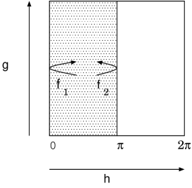
Figure 3: Double cover for annulus diagram

For the annulus case depicted in figure 3, we impose the path integral variable ${\cal X}$ to have the twisted boundary condition,

$${\cal X}(\sigma_{0},\sigma_{1}+2\pi)=h{\cal X}(\sigma_{0},\sigma_{1})\qquad{\cal X}(\sigma_{0}+2\pi,\sigma_{1})=g{\cal X}(\sigma_{0},\sigma_{1})$$ (3.6)

$g,h\in\Gamma$ should satisfy $g\cdot h=h\cdot g.$ We will identify it with ${\bf X}$ by (for $0\leq\sigma_{1}\leq\pi$)

$${\bf X}_{L}(\sigma_{0},\sigma_{1})={\cal X}(\sigma_{0},\sigma_{1}),\quad{\bf X}_{R}(\sigma_{0},\sigma_{1})=f_{2}\cdot{\cal X}(\sigma_{0},2\pi-\sigma_{1}).$$ (3.7)

With this assignment, ${\bf X}$ satisfies the boundary condition at $\sigma_{1}=\pi$ automatically. On the other hand, the boundary condition at $\sigma_{1}=0$ requires,

$${\bf X}_{R}(\sigma_{0},0)=f_{2}\cdot{\cal X}(\sigma_{0},2\pi)=f_{2}\cdot h\cdot{\cal X}(\sigma_{0},0).$$ (3.8)

Since the last formula should be same as $f_{1}\cdot{\cal X}(\sigma_{0},0)$,

$$h=f_{2}^{-1}\cdot f_{1}.$$ (3.9)

$h$ gives the actual twist in the open string sector and satisfies $h^{g}\equiv ghg^{-1}=h$.

The variant of the modular invariance in the open string case is that the annulus partition function can be alternatively expressed as the inner product between the boundary states. In the orbifold case, the boundary state depends on two elements $(g,f)$ in the group $\Gamma$. We will denote it as ${|\,B:g,f\rangle\!\rangle}$.

The first element $g$ specifies which twisted sector the closed string variable belongs to.

$$\left.(\overline{\bf X}({\overline{\sigma}}_{0},{\overline{\sigma}}_{1}+2\pi)-g\cdot\overline{\bf X}({\overline{\sigma}}_{0},{\overline{\sigma}}_{1}))\right|_{{\overline{\sigma}}_{0}=0}{|\,B:g,f\rangle\!\rangle}=0\,\,.$$ (3.10)

(We used different notations for embedding functions $\overline{\bf X}$ and world sheet coordinates $\sigma$ in order to explicitly shows that we are considering the closed string sector.) The second element $f$ specifies the twist at the boundary,

$$\left.(\overline{\bf X}_{R}({\overline{\sigma}}_{0},{\overline{\sigma}}_{1})-f\cdot\overline{\bf X}_{L}({\overline{\sigma}}_{0},{\overline{\sigma}}_{1}))\right|_{{\overline{\sigma}}_{0}=0}{|\,B:g,f\rangle\!\rangle}=0.$$ (3.11)

From the boundary conditions of the open string, we need to impose the constraints,

$$\left[g,f\right]=0\,\,,\quad f^{2}=1\,\,.$$ (3.12)

The modular transformation implies the relation,

$$\mbox{Tr}_{{\cal H}_{f_{1},f_{2}}}\left(g{\bf e}\!\left[\tau L_{0}^{open}\right]\right)\sim{\langle\!\langle B:g,f_{2}\,|}\,{\bf e}\!\left[-(1/2\tau)(L_{0}^{closed}+\bar{L}_{0}^{closed})\right]{|\,B:g,f_{1}\rangle\!\rangle}\,\,.$$ (3.13)

3.3 Möbius strip and cross-cap state

In Möbius diagram, we need to calculate the trace such as,

$$\mbox{Tr}_{{\cal H}_{f_{1},f_{2}}}\left(\Omega\,g\,{\bf e}\!\left[\tau L_{0}^{open}\right]\right)\,\,,$$ (3.14)

where $\Omega$ is the open string flip operator. As in the annulus case, we need to impose some constraints on $f_{1},f_{2},g\in\Gamma$ to have a non-vanishing result.

First let us investigate the action of $\Omega g$ on ${\cal H}_{f_{1},f_{2}}$. It acts on ${\bf X}_{L},{\bf X}_{R}$ as

$${\bf X}_{L} \longrightarrow {\bf Y}_{L}(\sigma_{0},\sigma_{1})\equiv g\cdot{\bf X}_{R}(\sigma_{0},\pi-\sigma_{1})$$

$${\bf X}_{R} \longrightarrow {\bf Y}_{R}(\sigma_{0},\sigma_{1})\equiv g\cdot{\bf X}_{L}(\sigma_{0},\pi-\sigma_{1}).$$ (3.15)

The boundary condition for the field ${\bf Y}$ becomes,

$${\bf Y}_{R}(\sigma_{0},0) = g{\bf X}_{L}(\sigma_{0},\pi)$$ (3.16)

$$= g\,f_{2}^{-1}\cdot{\bf X}_{R}(\sigma_{0},\pi)$$

$$= g\,f_{2}^{-1}\,g^{-1}\cdot{\bf Y}_{L}(\sigma_{0},0)$$

In other word, ${\bf X}\in{\cal H}_{f_{1},f_{2}}$ implies $\Omega\,g\cdot{\bf X}\in{\cal H}_{gf_{2}^{-1}g^{-1},gf_{1}^{-1}g^{-1}}$. In order to have non-vanishing trace (3.14), we need to impose these two Hilbert spaces are the same,

$$f_{2}=gf_{1}^{-1}g^{-1},\quad f_{1}=gf_{2}^{-1}g^{-1}.$$ (3.17)

If one examines these two conditions carefully, one may notice that $g,f_{1},f_{2}$ should satisfy further conditions,

$$\left[g^{2},f_{1}\right]=\left[g^{2},f_{2}\right]=0$$ (3.18)

To summarize, the non-vanishing Möbius strip amplitude is characterized by $g,f_{1}\in\Gamma$ with constraints,

$$f_{1}^{2}=1,\qquad\left[g^{2},f_{1}\right]=0\,\,.$$ (3.19)

$f_{2}$ is then determined from (3.17). The actual twist in the open string is given by,

$$h=f_{2}^{-1}\,f_{1}=g\,f_{1}\,g^{-1}\,f_{1}\,\,,$$ (3.20)

which satisfies the condition typical in unorientable cases, $h^{g}=h^{-1}$.

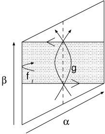
Figure 4: Double cover for Möbius diagram

In the standard double covering of Möbius strip (figure 4), these conditions are explained as follows. We introduce the path integral variable ${\cal X}$ satisfies the twisted boundary condition,

$${\cal X}(\sigma_{0}+\pi,\sigma+\pi) = \alpha\cdot{\cal X}(\sigma_{0},\sigma_{1})$$

$${\cal X}(\sigma_{0}+2\pi,\sigma) = \beta\cdot{\cal X}(\sigma_{0},\sigma_{1})\qquad\alpha,\beta\in\Gamma.$$ (3.21)

From this field, we would like to construct the left and right movers of the open string which satisfy the boundary condition,

$${\bf X}_{R}(\sigma_{0},0) = f_{1}\cdot{\bf X}_{L}(\sigma_{0},0)$$

$${\bf X}_{R}(\sigma_{0}+\pi,\pi/2) = g\cdot{\bf X}_{L}(\sigma_{0},\pi/2),$$

$${\bf X}_{L}(\sigma_{0}+\pi,\pi/2) = g\cdot{\bf X}_{R}(\sigma_{0},\pi/2).$$ (3.22)

The boundary conditions in the second and the third lines are (twisted) cross-cap type conditions. It is consistent with (3.3) only when $\beta=g^{2}$.

We use the following identification between ${\bf X}$ and ${\cal X}$,

$${\bf X}_{L}(\sigma_{0},\sigma_{1}) = {\cal X}(\sigma_{0},\sigma_{1})$$

$${\bf X}_{R}(\sigma_{0},\sigma_{1}) = f_{3}\cdot{\cal X}(\sigma_{0}+\pi,\pi-\sigma_{1}).$$ (3.23)

Boundary condition at $\sigma_{1}=\pi/2$ implies,

$${\bf X}_{R}(\sigma_{0}+\pi,\pi/2) = f_{3}\cdot{\cal X}(\sigma_{0}+2\pi,\pi/2)$$

$$= f_{3}\,g^{2}\cdot{\cal X}(\sigma_{0},\pi/2)$$

$$g\cdot{\bf X}_{L}(\sigma_{0},\pi/2) = g\cdot{\cal X}(\sigma_{0},\pi/2).$$ (3.24)

Namely,

$$f_{3}=g^{-1}.$$ (3.25)

Similarly boundary condition at $\sigma_{1}=0$ is consistent with (3.3) only when,

$$\alpha=g\,f_{1}$$ (3.26)

Periodicity and the twisted boundary condition along $\sigma_{1}=0$ implies,

$$\left[f_{1},\beta\right]=\left[f_{1},g^{2}\right]=0.$$ (3.27)

This calculation can be summarized by the introduction of the cross-cap state ${|\,C:g,f\rangle\!\rangle}$ which satisfies,

$$(\overline{\bf X}_{L}(0,{\overline{\sigma}}_{1}+\pi)-f\cdot\widetilde{\bf X}_{R}(0,{\overline{\sigma}}_{1})){|\,C:g,f\rangle\!\rangle} = 0$$

$$(\overline{\bf X}_{R}(0,{\overline{\sigma}}_{1}+\pi)-f\cdot\widetilde{\bf X}_{L}(0,{\overline{\sigma}}_{1})){|\,C:g,f\rangle\!\rangle} = 0$$ (3.28)

The twisted boundary condition of the closed string is specified by $g$. However, it is clear that these conditions automatically implies that $\overline{\bf X}$ belongs to the twisted sector defined by $f^{2}$,

$$\overline{\bf X}({\overline{\sigma}}_{0},{\overline{\sigma}}_{1}+2\pi)=f^{2}\cdot\overline{\bf X}({\overline{\sigma}}_{0},{\overline{\sigma}}_{1}).$$ (3.29)

Namely we always have $g=f^{2}$. The modular transformation of Möbius strip can be now written as

$$\mbox{Tr}_{{\cal H}_{f_{1},f_{1}^{g}}}\left(g\,{\bf e}\!\left[\tau L_{0}^{open}\right]\right)={\langle\!\langle B:g^{2},f_{1}\,|}\,{\bf e}\!\left[-(1/8\tau)(L_{0}^{closed}+\bar{L}_{0}^{closed})\right]{|\,C:g^{2},g\rangle\!\rangle}.$$ (3.30)

3.4 Klein bottle

In the Klein bottle amplitude, we need to evaluate

$${\mbox{Tr}}_{{\cal H}_{h}}\left(\Omega^{closed}\,g\,{\bf e}\!\left[\tau(L_{0}^{closed}+\bar{L}_{0}^{closed})\right]\right)$$ (3.31)

As in the Möbius strip case,

$${\bf X}\in{\cal H}_{h}\rightarrow\Omega^{closed}g{\bf X}\in{\cal H}_{gh^{-1}g^{-1}}.$$ (3.32)

Therefore, to have non-vanishing trace, we need impose constraint on $g,h$,

$$h=gh^{-1}g^{-1}\quad\mbox{or}\quad hg=gh^{-1}.$$ (3.33)

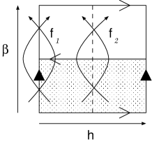
Figure 5: Double cover for Klein bottle diagram

In the double covering (figure 5), we define a chiral field ${\cal X}$ which has twisted boundary condition,

$${\cal X}(\sigma_{0},\sigma_{1}+2\pi)=h\cdot{\cal X}(\sigma_{0},\sigma_{1}),\quad{\cal X}(\sigma_{0}+2\pi,\sigma_{1})=\beta\cdot{\cal X}(\sigma_{0},\sigma_{1}).$$ (3.34)

${\bf X}$ satisfies cross-cap type boundary condition at $\sigma_{1}=0,\pi$,

$${\bf X}_{R,L}(\sigma_{0}+\pi,0)=f_{1}{\bf X}_{L,R}(\sigma_{0},0)\quad{\bf X}_{R,L}(\sigma_{0}+\pi,\pi)=f_{2}{\bf X}_{L,R}(\sigma_{0},\pi)$$ (3.35)

We identify

$${\bf X}_{L}(\sigma_{0},\sigma_{1})={\cal X}(\sigma_{0},\sigma_{1})\quad{\bf X}_{R}(\sigma_{0},\sigma_{1})=f_{2}\cdot{\cal X}(\sigma_{0}-\pi,2\pi-\sigma_{1})$$ (3.36)

It automatically satisfies boundary condition at $\sigma_{1}=\pi$. Boundary condition at $\sigma_{1}=0$ is satisfied if

$$h=f_{2}^{-1}f_{1}.$$ (3.37)

Twist in time direction requires,

$$\beta=f_{1}^{2}=f_{2}^{2}.$$ (3.38)

If we identify $g=f_{1}$, two conditions (3.33) and (3.38) are equivalent. The modular invariance in this case can be written as,

$$\mbox{Tr}_{{\cal H}_{h}}\left(g\,\Omega^{closed}\,{\bf e}\!\left[\tau(L_{0}+\bar{L}_{0})\right]\right)={\langle\!\langle C:f_{2}^{2},f_{2}\,|}\,{\bf e}\!\left[-(1/4\tau)(L_{0}+\bar{L}_{0})\right]{|\,C:f_{1}^{2},f_{1}\rangle\!\rangle}$$ (3.39)

with $g=f_{1}$ and $h=f_{2}^{-1}f_{1}$.

4 Classification of irreducible boundary conditions

In this section, we explicitly solve the constraints of the twists in the previous section for three diagrams. We classify all the possible irreducible solutions together with the free parameters. Our result in this section is summarized in the following theorem.

Theorem 2
(i) Klein bottle: irreducible solutions for (3.33) are given by,

$$h=diag(\overbrace{{\cal T}_{n},\cdots,{\cal T}_{n}}^{m})\,\,,\quad g=diag({\cal T}_{n}^{p_{0}}{\cal S}_{n},\cdots,{\cal T}_{n}^{p_{m-1}}{\cal S}_{n})\cdot{\overline{\cal T}}_{m},$$ (4.1)

where ${\cal S}_{n}$ is the inversion permutation of $n$ elements $(n-1,n-2,n-3,\cdots,0)$. $p_{i}$ ($i\equiv 0,\cdots,m-1$ mod $m$) takes their values in $0,1,\cdots,n-1$ (mod $n$). We will refer this solution as (K). (ii) Annulus: there are three types of the irreducible solutions for (3.5,3.9) together with $f_{i}^{2}=1$.

• ($I_{A}$):

  $$h = diag(\overbrace{{\cal T}_{n},\cdots,{\cal T}_{n}}^{m})$$

  $$g = diag({\cal T}_{n}^{p_{0}},\cdots,{\cal T}_{n}^{p_{m-1}})\cdot{\overline{\cal T}}_{m},$$

  $$f_{1} = diag({\cal T}_{n}^{q_{0}}{\cal S}_{n},\cdots,{\cal T}_{n}^{q_{m-1}}{\cal S}_{n}),$$

  $$f_{2} = diag({\cal T}_{n}^{q_{0}+1}{\cal S}_{n},\cdots,{\cal T}_{n}^{q_{m-1}+1}{\cal S}_{n}).$$ (4.2)

  $p_{i},q_{i}$ ($i\equiv 0,\cdots,m-1$ mod $m$) takes their values in $0,1,\cdots,n-1$ (mod $n$). They should satisfy the constraint,

  $$q_{\ell}-q_{\ell+1}\equiv 2p_{\ell},\quad(\ell=0,\cdots,n-1\mbox{ mod}\,\,\,n)$$ (4.3)

• ($II_{A}$): for even $m$, with the same $h,g$ as in (• ‣ 4), together with

  $$f_{1} = diag({\cal T}_{n}^{q_{0}}{\cal S}_{n},\cdots,{\cal T}_{n}^{q_{m-1}}{\cal S}_{n})({\overline{\cal T}}_{(m)})^{m/2},$$

  $$f_{2} = diag({\cal T}_{n}^{q_{0}+1}{\cal S}_{n},\cdots,{\cal T}_{n}^{q_{m-1}+1}{\cal S}_{n})({\overline{\cal T}}_{(m)})^{m/2},$$ (4.4)

  with $q_{k}=q_{k+m/2}$. The constraint for $p,q$ are given by

  $$q_{\ell}-q_{\ell+1}\equiv p_{\ell}+p_{\ell+m/2}\quad(\mbox{mod}\,\,n)$$ (4.5)

  $\ell$ in this equation is defined in modulo $m$.

• ($\widetilde{II}_{A}$): for even $m$, with the same $h,f_{1},f_{2}$ as in ($II_{A}$), together with

  $$g=diag({\cal T}_{n}^{p_{0}},\cdots,{\cal T}_{n}^{p_{m-1}})diag({\overline{\cal T}}_{m/2},{\overline{\cal T}}_{m/2}).$$ (4.6)

  The constraint for $p,q$ are given by

  $$q_{\ell}-q_{\ell+1}\equiv p_{\ell}+p_{\ell+m/2}\quad(\mbox{mod}\,\,n)$$ (4.7)

  The index $\ell$ in this equation is defined in modulo $m/2$.

(iii) Möbius strip: there are three types of the irreducible solutions for (3.19,3.20).

• ($I_{M}$):

  $$h = diag(\overbrace{{\cal T}_{n},\cdots,{\cal T}_{n}}^{m})$$

  $$g = diag({\cal T}_{n}^{p_{0}}{\cal S}_{n},\cdots,{\cal T}_{n}^{p_{m-1}}{\cal S}_{n})\cdot{\overline{\cal T}}_{m},$$

  $$f_{1} = diag({\cal T}_{n}^{q_{0}}{\cal S}_{n},\cdots,{\cal T}_{n}^{q_{m-1}}{\cal S}_{n}).$$ (4.8)

  The constraint for $p,q$ is

  $$q_{\ell}+q_{\ell+1}\equiv 2p_{\ell}-1,\quad(\ell=0,\cdots,n-1\mbox{ mod\,}n)$$ (4.9)

• ($II_{M}$): for even $m$, with the same $h,g$ as in (• ‣ 4), together with

  $$f_{1}=diag({\cal T}_{n}^{q_{0}}{\cal S}_{n},\cdots,{\cal T}_{n}^{q_{m-1}}{\cal S}_{n})({\overline{\cal T}}_{(m)})^{m/2}.$$ (4.10)

  The constraint for $p,q$ are given by

  $$q_{\ell}+q_{\ell+1}\equiv p_{\ell}+p_{\ell+m/2}-1\quad(\mbox{mod}\,\,n)$$ (4.11)

  $\ell$ in this equation is defined in modulo $m$.

• ($\widetilde{II}_{M}$): for even $m$, with the same $h,f_{1}$ as in ($II_{M}$), together with

  $$g=diag({\cal T}_{n}^{p_{0}}{\cal S}_{n},\cdots,{\cal T}_{n}^{p_{m-1}}{\cal S}_{n})\cdot diag({\overline{\cal T}}_{m/2},{\overline{\cal T}}_{m/2}).$$ (4.12)

  The constraint for $p,q$ are given by

  $$q_{\ell}+q_{\ell+1}\equiv p_{\ell}+p_{\ell+m/2}-1\quad(\mbox{mod}\,\,n)$$ (4.13)

  The index $\ell$ in this equation is defined in modulo $m/2$.

While ${\cal T}_{n}^{p}$ represents the cyclic rotation of string bits in length $n$ long string, ${\cal S}_{n}$ flips the orientation of the long string. Four sectors, $(II_{A})$, $(\widetilde{II}_{A})$, $(II_{M})$, $(\widetilde{II}_{M})$, can be interpreted as giving the closed string sectors with/without orientation flip which appears in open string sector.

The rest of this section is devoted to straightforward but rather lengthy proof of this theorem. Before we embark on the calculation of indivisual cases, we first mention a simple lemma

Lemma 1: In the irreducible sets, $h$ should always be the direct product of the cyclic permutations of the same length $n$. Proof: We already mentioned that for each diagram, $h$ and $g$ satisfy,

$$h^{g}= h,$$ Annulus

$$h^{g}= h^{-1}, \qquad\mbox{Klein bottle, M\"{o}bius strip},$$ (4.14)

where $h^{g}\equiv ghg^{-1}$. Let us assume that the conjugacy class of $h$ is given by the partition $(n)(m)$ with $n\neq m$. LHS of (4) belongs to the same conjugacy class with each element permuted by $g$. Since $n\neq m$, $g$ can not mix elements in $(n)$ and $(m)$.

For open string sectors (Annulus and Möbius), we also determine $f_{i}$ ($i=1,2$) with $f_{i}^{2}=1$ and $h=f_{2}^{-1}\,f_{1}$. Because of $f_{i}^{2}=1$, one may easily derive that $h^{f_{1}}=h^{-1}$. By repeating our argument on $g$, $f_{1}$ (and also $f_{2}$) can not mix the elements in $(n)$ and $(m)$.

It proved that when $h=(n)(m)$ with $n\neq m$, there are no the irreducible sets. QED

4.1 Klein bottle

From lemma 1, we may restrict $h,g$ to the following form,

$$h=diag(\overbrace{{\cal T}_{n},\cdots,{\cal T}_{n}}^{m}),\quad g=diag(\alpha_{0},\cdots,\alpha_{m-1})\cdot{\overline{\cal T}}_{m},$$ (4.15)

where $\alpha_{\ell}$ is any permutations of $n$ elements. $h^{g}=h^{-1}$ implies, $\alpha_{\ell}{\cal T}_{n}\alpha_{\ell}^{-1}={\cal T}_{n}^{-1}$. To derive conditions in (K), it is enough to prove the following lemma, Lemma 2: The general solution to

$$g{\cal T}_{n}g^{-1}={\cal T}_{n}^{-1},$$ (4.16)

is given by $g={\cal T}_{n}^{p}{\cal S}_{n}$ for $p=0,1,\cdots,n$. Proof: Assume that $g$ maps $(0,1,2,\cdots,n-1)$ to $(g_{0},g_{1},\cdots,g_{n-1})$. $g{\cal T}_{n}={\cal T}_{n}^{-1}g$ implies

$$g(i+1)-g(i)+1\equiv 0\quad\mbox{mod}\,n.$$ (4.17)

General solution to this difference equation is clearly (4.16). QED.

4.2 Annulus

Because $\left[h,g\right]=0$, we may write general irreducible solutions in the following form,

$$h = diag(\overbrace{{\cal T}_{n},\cdots,{\cal T}_{n}}^{m})$$

$$g = diag({\cal T}_{n}^{p_{0}},\cdots,{\cal T}_{n}^{p_{m-1}})\cdot G,$$

$$f_{i} = diag(\alpha^{(i)}_{1},\cdots,\alpha^{(i)}_{m-1})\cdot F_{i}.$$ (4.18)

where $G$ and $F_{i}$ belong to $S_{m}$. The constraints $\left[g,f_{i}\right]=0$, $h=f_{2}^{-1}f_{1}$ and $f_{i}^{2}=1$ implies,

$$\left[G,F_{i}\right] = 0$$

$$F_{1}^{2}=F_{2}^{2}=F_{1}\,F_{2} = 1.$$ (4.19)

The equation in the second line implies $F_{1}=F_{2}$. We can use Lemma 1 to show that $G$ is written as a direct product of the cyclic permutations of the same length $({\overline{\cal T}}_{m/s})^{\otimes s}$ if we use the irreducibility. From the first equation, $s$ must be either 1 or 2. If $s=1$, $F_{i}$ can be either 1 ($I_{A}$),

$$G={\overline{\cal T}}_{m}\,\,\,\qquad F=1_{m},$$ (4.20)

or ${\overline{\cal T}}_{m/2}$ if $m$ is even ($II_{A}$)

$$G={\overline{\cal T}}_{m}\,\,\,\qquad F=G^{m/2}=\left(\begin{array}[]{c c}0&1_{m/2}\\ 1_{m/2}&0\end{array}\right)\,\,\,,$$ (4.21)

If $s=2$, $G$ and $F_{i}$ must be the following form ($\widetilde{II}_{A}$),

$$G=\left(\begin{array}[]{c c}{\overline{\cal T}}_{m/2}&0\\ 0&{\overline{\cal T}}_{m/2}\end{array}\right)\,\,\,,\quad F=\left(\begin{array}[]{c c}0&1_{m/2}\\ 1_{m/2}&0\end{array}\right)\,\,\,,$$ (4.22)

with even $m$.

4.2.1 $I_{A}$

$f_{i}^{2}=1$ and $f_{2}^{-1}f_{1}=h$ implies

$$(\alpha_{\ell}^{(2)})^{-1}\,\alpha_{\ell}^{(1)}={\cal T}_{n},\qquad(\alpha_{\ell}^{(i)})^{2}=1.$$ (4.23)

(• ‣ 4) is easily derived by using the following lemma. (4.3) comes from the constraint $\left[f_{i},g\right]=0$.

Lemma 3: For $f_{1},f_{2}\in S_{n}$, the general solution to

$$f_{1}^{2}=f_{2}^{2}=1,\quad f_{2}^{-1}f_{1}={\cal T}_{n}$$ (4.24)

is given by

$$f_{1}={\cal T}_{n}^{p}{\cal S}_{n},\quad f_{2}={\cal T}_{n}^{p+1}{\cal S}_{n},\quad p=0,\cdots,n-1\quad\mbox{mod}\,\,n.$$ (4.25)

Proof: If we write $f_{2}^{-1}f_{1}=h$ and $f_{1}=g$,

$$h^{g}=f_{1}\,f_{2}=h^{-1}={\cal T}_{n}^{-1}.$$ (4.26)

This is exactly the same condition as Lemma 2. It permits us to write $f_{i}$ in the form (4.25). By using the relation,

$${\cal T}_{n}^{p}{\cal S}_{n}={\cal S}_{n}{\cal T}_{n}^{-p},$$ (4.27)

it is straightforward to prove that $f_{i}$s thus defined satisfy $f_{i}^{2}=1$. QED.

4.2.2 $II_{A}$, $\widetilde{II}_{A}$

We write $m/2\equiv k$. The constraints $f_{i}^{2}=1$ are written in components, $\alpha^{(i)}_{\ell}\alpha^{(i)}_{\ell+k}=1$, namely $\alpha^{(i)}_{\ell+k}=(\alpha^{(i)})^{-1}_{\ell}$. By plugging it into $f_{2}^{-1}f_{1}=h$, we get

$$\alpha_{\ell}^{(2)}(\alpha_{\ell}^{(1)})^{-1}=(\alpha_{\ell}^{(2)})^{-1}\alpha_{\ell}^{(1)}={\cal T}_{n}.$$

From this equation, it is not difficult to prove $\alpha_{\ell}^{(i)}{\cal T}_{n}\alpha_{\ell}^{(i)\,-1}={\cal T}_{n}^{-1}$. By using lemma 2, we conclude that $f_{i}$ must be of the form, (• ‣ 4). Finally constraints (4.5,4.7) are obtained by imposing $\left[g,f_{i}\right]=0$.

4.3 Möbius

With the help of Klein bottle calculation, one may seek the general irreducible solution in the following form,

$$h = diag(\overbrace{{\cal T}_{n},\cdots,{\cal T}_{n}}^{m})$$

$$g = diag({\cal T}_{n}^{p_{0}}{\cal S}_{n},\cdots,{\cal T}_{n}^{p_{m-1}}{\cal S}_{n})\cdot G\,\,\,,$$

$$f_{1} = diag(\alpha_{0},\cdots,\alpha_{m-1})\cdot F_{1}\,\,,$$ (4.28)

with $G,F_{1}\in S_{m}$. In this form $h^{g}=h^{-1}$ is automatically satisfied. (3.19,3.20) lead to

$$\left[F_{1},G\right]=0\,,\quad F_{1}^{2}=1\,.$$ (4.29)

This is exactly the same constraint in the annulus (4.2). We may use the same solutions, (4.20,4.21,4.22) and call the solutions associated with each of them as $I_{M}$, $II_{M}$, $\widetilde{II}_{M}$.

4.3.1 $I_{M}$

$f_{1}^{2}=1$ implies $\alpha_{\ell}^{2}=1$. Constraint (3.20) gives

$${\cal T}_{n}^{p_{\ell}}{\cal S}_{n}\alpha_{\ell}^{-1}{\cal T}_{n}^{p_{\ell}}{\cal S}_{n}\alpha_{\ell+1}={\cal T}_{n}.$$ (4.30)

Since $\alpha_{\ell}^{2}=1$ and $({\cal T}_{n}^{p_{\ell}}{\cal S}_{n}\alpha_{\ell}^{-1}{\cal T}_{n}^{p_{\ell}}{\cal S}_{n})^{2}=1$, lemma 3 permits us to write

$$\alpha_{\ell}={\cal T}_{n}^{q_{\ell}}{\cal S}_{n}\,\,,$$ (4.31)

which proved (• ‣ 4). The constraint (4.3) comes from putting this value into (4.30) again.

4.3.2 $II_{M}$ and $\widetilde{II}_{M}$

In these cases, $f_{1}$ has the following form ($m=2k$),

$$f_{1}=diag(\alpha_{0},\cdots,\alpha_{m-1})\cdot({\overline{\cal T}}_{2k})^{k}.$$ (4.32)

$f_{1}^{2}=1$ gives $\alpha_{\ell+k}=\alpha_{\ell}^{-1}$. We note that $f_{2}=(f_{1})^{g}$ have the same form. As in the $II_{A}$ case, one can show that $\alpha_{\ell}$ have the following form,

$$\alpha_{\ell}={\cal T}_{n}^{q_{\ell}}{\cal S}_{n}\,\,.$$ (4.33)

(3.20) gives the same type of constraint in both $II_{M}$ and $\widetilde{II}_{M}$,

$$({\cal T}_{n}^{p_{\ell}}{\cal S}_{n})\,\alpha_{\ell}\,({\cal T}_{n}^{p_{k+\ell}}{\cal S}_{n})\,\alpha_{\ell+1}^{-1}={\cal T}_{n}\,\,,$$ (4.34)

which gives (4.11,4.13).

The proof of theorem 2 is completed.

5 Partition functions

In this section, we explicitly calculate the partition functions for the irreducible boundary conditions discussed in previous section. One interesting feature is that the sectors for the long strings are in general different from those of the short strings. Actually this is clear since we already mentioned there are the long closed string sectors in the annulus or Möbius strip amplitude in the short string.

Since the correspondence looks rather complicated, we summarize our result in the following table.

Short string sector	$n$	$m$	Long string sector	Partition function
KB	$*$	odd	Klein Bottle	${\cal Z}^{KB}(\tau_{n,m,0})$
	$*$	even	Torus	${\cal Z}^{T}(\tau_{n,m,p},\bar{\tau}_{n,m,p})$
Annulus: $I_{A}$	odd	$*$	Annulus	${\cal Z}^{A}(\tau_{n,m,0})$
	even	$*$	Annulus+Möbius	${\cal Z}^{A}(\tau_{n,m,0})+{\cal Z}^{M}(\tau_{n,m,0})$
Annulus: $II_{A}$	$*$	$2\times*$	Klein Bottle	${\cal Z}^{KB}(\tau_{n,m/2,0})$
Annulus: $\widetilde{II}_{A}$	$*$	$2\times*$	Torus	${\cal Z}^{T}(\tau_{n,m/2,p},\bar{\tau}_{n,m/2,p})$
Möbius: $I_{M}$	odd	odd	Möbius	${\cal Z}^{M}(\tau_{n,m,0})$
	odd	even	Annulus	${\cal Z}^{A}(\tau_{n,m,0})$
	even	even	Annulus+Möbius	${\cal Z}^{A}(\tau_{n,m,0})+{\cal Z}^{M}(\tau_{n,m,0})$
	even	odd	—	0
Möbius: $II_{M}$	$*$	$2\times$odd	Torus	${\cal Z}^{T}(\tau_{n,m/2,p^{*}},\bar{\tau}_{n,m/2,p^{*}})$
	$*$	$2\times$even	Klein Bottle	${\cal Z}^{KB}(\tau_{n,m/2,0})$
Möbius: $\widetilde{II}_{M}$	$*$	$2\times$even	Torus	${\cal Z}^{T}(\tau_{n,m/2,p},\bar{\tau}_{n,m/2,p})$
	$*$	$2\times$odd	Klein Bottle	${\cal Z}^{KB}(\tau_{n,m/2,0})$

For Klein Bottle/Annuls/Möbius strip cases, the moduli parameter $\tau$ is pure imaginary. $\tau_{n,m,p}$ is the long string moduli (2.27). $p$ is an integer from $0$ to $n-1$ and $p^{*}$ is the half-odd integer from $0$ to $n$.

In this table we used the partition functions for a single string in each sector. We will first prove this table by employing the explicit operator formalism for the simplest target space ${\bf R}^{1}$. In this case, they have the following standard form,

$${\cal Z}^{T}(\tau,\bar{\tau}) = \frac{{\bf e}\!\left[-(\tau-\bar{\tau}))/24\right]}{\sqrt{\mbox{Im}\,\tau}}\prod_{n=1}^{\infty}\left((1-{\bf e}\!\left[n\tau\right])(1-{\bf e}\!\left[-n\bar{\tau}\right])\right)^{-1}\,\,,$$ (5.1)

$${\cal Z}^{KB}(\tau) = \frac{{\bf e}\!\left[-\tau/12\right]}{\sqrt{\mbox{Im}\,\tau}}\prod_{n=1}^{\infty}\left(1-{\bf e}\!\left[2n\tau\right]\right)^{-1}\,\,,$$ (5.2)

$${\cal Z}^{A}(\tau) = \frac{{\bf e}\!\left[-\tau/24\right]}{\sqrt{2\mbox{Im}\,\tau}}\prod_{n=1}^{\infty}\left(1-{\bf e}\!\left[n\tau\right]\right)^{-1}\,\,,$$ (5.3)

$${\cal Z}^{M}(\tau) = \frac{{\bf e}\!\left[-\tau/24\right]}{\sqrt{2\mbox{Im}\,\tau}}\prod_{n=1}^{\infty}\left(1-(-1)^{n}{\bf e}\!\left[n\tau\right]\right)^{-1}\,\,.$$ (5.4)

In the first subsection, we give the examination of this table by using the explicit operator formalism. In the most cases, we omit the analysis of the momentum integration since they are the same as our discussion in section 2.

In the second subsection, we present a different proof based on multiple cover of the world sheets. This is similar to our discussion in the section 2.2.2 and can be applied to the arbitrary target space. Although it may be less rigorous compared to the analysis by the operator formalism, it is much better to explain the topological nature of this table.

5.1 Analysis by Operator formalism

5.1.1 Klein Bottle

As in our calculation in the torus amplitude, we make the discrete Fourier transformation (2.16) for the component fields. The action of $h$ was determined in (2.2.1) and it is possible to use the same mode expansion (2.19). One novelty is to determine the action of ${\cal S}_{n}$,

$$({\cal S}_{n}\cdot\widetilde{\bf X})^{a,J} = \frac{1}{\sqrt{n}}\sum_{I=0}^{n-1}{\bf e}\!\left[-\frac{aI}{n}\right]{\bf X}^{n-I-1,J}$$ (5.5)

$$= {\bf e}\!\left[\frac{a}{n}\right]\widetilde{\bf X}^{-a,J}\,\,.$$

The action of $g$ in (4.1) is evaluated as,

$$(g\cdot\widetilde{\bf X})^{a,J}={\bf e}\!\left[\frac{ap_{J}}{n}\right]\widetilde{\bf X}^{-a,J+1}.$$ (5.6)

Since the orientation flip interchange the left and the right movers, $(\Omega\cdot g)$ acts on the oscillators as

$$(\Omega\cdot g)\,\alpha_{r-a/n}^{a,J} = {\bf e}\!\left[\frac{ap_{J}}{n}\right]\tilde{\alpha}_{r-a/n}^{-a,J+1}\,$$

$$(\Omega\cdot g)\,\tilde{\alpha}_{r-a/n}^{-a,J} = {\bf e}\!\left[\frac{-ap_{J}}{n}\right]\alpha_{r-a/n}^{a,J+1}\,.$$ (5.7)

We need to find a combination of the left and right movers which is invariant up to scalar multiplication under $\Omega\cdot g$. To this end, we define a linear combination

$$\beta^{a}_{r-a/n}=\sum_{J=0}^{m-1}C_{J}\alpha^{a,J}_{r-a/n},$$ (5.8)

and define $\tilde{\beta}^{a}_{r-a/n}\equiv(\Omega\,g)\,\beta^{a}_{r-a/n}$. If one can find appropriate coefficients $C_{J}$ such that $\beta$ satisfies

$$\Omega\,g\cdot\tilde{\beta}^{a}_{r-a/n}=\lambda\beta^{a}_{r-a/n}\,\,,$$ (5.9)

$\beta^{a}_{r-a/n}\tilde{\beta}^{a}_{r-a/n}$ becomes diagonal under the action of $\Omega\,g$,

$$\Omega\,g\left(\beta^{a}_{r-a/n}\tilde{\beta}^{a}_{r-a/n}\right)=\lambda\left(\beta^{a}_{r-a/n}\tilde{\beta}^{a}_{r-a/n}\right)\,\,.$$ (5.10)

In terms of $C_{J}$, (5.9) becomes

$$\lambda C_{J+2}=C_{J}{\bf e}\!\left[\frac{a}{n}(p_{J}-p_{J+1})\right]\,\,.$$ (5.11)

Since $J$ takes its value in $0,\cdots,m-1$ (modulo $m$), the solution becomes essentially different depending on whether $m$ is even or odd. [1] odd $m$:

In this case, the recursion relation gives

$$C_{2m} = \frac{1}{\lambda}{\bf e}\!\left[\frac{a}{n}(p_{2m-2}-p_{2m-1})\right]C_{2(m-1)}$$ (5.12)

$$= \cdots$$

$$= \frac{1}{\lambda^{m}}{\bf e}\!\left[\frac{a}{n}\left(\sum_{\ell=0}^{m-1}p_{2m-2\ell}-\sum_{\ell=0}^{m-1}p_{2m-1-2\ell}\right)\right]\,C_{0}$$

$$= \frac{1}{\lambda^{m}}\,C_{0}\,\,.$$

$C_{2m}=C_{0}$ implies $\lambda={\bf e}\!\left[\frac{b}{m}\right]$ with $b=0,1,\cdots m-1$.

Along the same line of calculation (2.2.1), we obtain the oscillator contribution to the partition function of Klein bottle,

$$\mbox{Tr}_{{\cal H}_{h}}(\Omega\,g\,{\bf e}\!\left[\tau(L_{0}+\bar{L}_{0})\right]) = \prod_{s=1}^{\infty}\prod_{a=0}^{n-1}\prod_{b=0}^{m-1}\frac{1}{1-{\bf e}\!\left[\frac{b}{m}+2\tau\left(s-\frac{a}{n}\right)\right]}$$ (5.13)

$$= \prod_{s=1}^{\infty}\prod_{a=0}^{n-1}\frac{1}{1-{\bf e}\!\left[2m\tau\left(s-\frac{a}{n}\right)\right]}$$

$$= \prod_{s=1}^{\infty}\frac{1}{1-{\bf e}\!\left[\frac{2m\tau}{n}\right]}\,\,.$$

The calculation of the zero mode contribution is the same as the torus. It proved the table.

[2] even $m$:

In this case, the recursion relation is split into two sequences $\left\{C_{\ell}\right\}_{\ell_{even}}$ and $\left\{C_{\ell}\right\}_{\ell_{odd}}$. The first one can be solved as,

$$C_{m}=\frac{1}{\lambda^{m/2}}{\bf e}\!\left[\frac{ap}{n}\right]\,C_{0}\,\,.$$ (5.14)

with

$$p=\sum_{\ell=0}^{m/2-1}p_{m-2\ell}-\sum_{\ell=0}^{m/2-1}p_{m-1-2\ell}\,\,.$$ (5.15)

It gives quantized eigenvalues for $\lambda$,

$$\lambda_{even}^{a,b}={\bf e}\!\left[\frac{2b}{m}+\frac{2ap}{nm}\right]\,\,,\quad b=0,\cdots,\frac{m}{2}-1\,\,.$$ (5.16)

Similarly, the recursion relation for $\left\{C_{\ell}\right\}_{\ell_{odd}}$, gives

$$\lambda_{odd}^{a,b}={\bf e}\!\left[\frac{2b}{m}-\frac{2ap}{nm}\right]\,\,,\quad b=0,\cdots,\frac{m}{2}-1\,\,.$$ (5.17)

The calculation of the partition function is now completely parallel to (2.2.1),

$$\mbox{Tr}_{{\cal H}_{h}}(\Omega\,g\,{\bf e}\!\left[\tau(L_{0}+\bar{L}_{0})\right]) = \prod_{s=1}^{\infty}\prod_{a=0}^{n-1}\prod_{b=0}^{m/2-1}\left(1-{\bf e}\!\left[\frac{2b}{m}-\frac{2ap}{nm}+2\tau\left(s-\frac{a}{n}\right)\right]\right)^{-1}$$ (5.18)

$$\cdot\left(1-{\bf e}\!\left[\frac{2b}{m}+\frac{2ap}{nm}+2\tau\left(s-\frac{a}{n}\right)\right]\right)^{-1}$$

$$= \prod_{s=1}^{\infty}\left(1-{\bf e}\!\left[\frac{m\tau-p}{n}s\right]\right)^{-1}\left(1-{\bf e}\!\left[\frac{m\tau+p}{n}s\right]\right)^{-1}$$

Together with the zero mode contribution, this is exactly the same as (2.29) except for that the short string moduli $\tau$ is pure imaginary. Interestingly the moduli for the long string $\tau_{n,m,p}$ has the real part as $p/n$.

5.1.2 Annulus

$I_{A}$

From the data (• ‣ 4), the mode expansion that satisfies the boundary conditions (3.2) at the two boundaries is given by,

$$\widetilde{\bf X}^{a,J}_{L} = i\sum_{s\in{\bf Z}}\frac{1}{s-a/n}\alpha^{a,J}_{s-a/n}{\bf e}\!\left[\sigma_{1}(-s+a/n)\right]$$

$$\widetilde{\bf X}^{a,J}_{R} = i{\bf e}\!\left[\frac{aq_{J}}{n}\right]\sum_{s\in{\bf Z}}\frac{1}{s+a/n}\alpha^{-a,J}_{s+a/n}{\bf e}\!\left[\sigma_{1}(s+a/n)\right]\,\,.$$ (5.19)

The action of $g$ on the other hand is given by,

$$\left(g\cdot\widetilde{\bf X}_{L}\right)^{a,J}={\bf e}\!\left[\frac{ap_{J}}{n}\right]\widetilde{\bf X}^{a,J+1}_{L}=i{\bf e}\!\left[\frac{ap_{J}}{n}\right]\sum_{s\in{\bf Z}}\frac{1}{s-a/n}\alpha^{a,J+1}_{s-a/n}{\bf e}\!\left[\sigma_{1}(-s+a/n)\right]\,\,.$$ (5.20)

Comparing these two equations, one gets the action of $g$ on the oscillators,

$$(g\cdot\alpha_{s-a/n})^{a,J}={\bf e}\!\left[\frac{ap_{J}}{n}\right]\alpha^{a,J+1}_{s-a/n}\,\,.$$ (5.21)

Since this is the same expression that we met in torus amplitude, one obtain the partition function immediately.

Unlike the torus case, $p=\sum_{J}p_{J}$ cannot take arbitrary integer. By summing over $J$ in (4.3), one obtains $2p\equiv 0$ modulo $n$. When $n$ is odd, $p=0$ is the only solution. Putting $p=0$, one obtains the standard annulus contribution of one long open string,

$$\mbox{Tr}_{{\cal H}_{f_{1},f_{2}}}\left(g{\bf e}\!\left[\tau\,L_{0}\right]\right)=\prod_{r=0}^{\infty}\frac{1}{1-{\bf e}\!\left[\frac{m\tau}{n}r\right]}\,\,.$$ (5.22)

On the other hand, when $n$ is even, we have two solutions, $p=0,\frac{n}{2}$. The first one is the annulus. The second solution gives,

$$\prod_{r=1}^{\infty}\frac{1}{1+{\bf e}\!\left[\frac{m\tau}{n}r+\frac{r}{2}\right]}=\prod_{r=1}^{\infty}\frac{1}{1+(-1)^{r}{\bf e}\!\left[\frac{m\tau}{n}r\right]}.$$ (5.23)

This is the standard Möbius strip amplitude for a long string.

$II_{A}$ and $\widetilde{II}_{A}$

In these cases we write $m=2k$ since $m$ must be even. The mode expansion and $g$ action is almost the same as $I_{A}$ case,

$$\widetilde{\bf X}^{a,J}_{L} = i\sum_{s\in{\bf Z}}\frac{1}{s-a/n}\alpha^{a,J}_{s-a/n}{\bf e}\!\left[\sigma_{1}(-s+a/n)\right]$$

$$\widetilde{\bf X}^{a,J}_{R} = i{\bf e}\!\left[\frac{aq_{J}}{n}\right]\sum_{s\in{\bf Z}}\frac{1}{s+a/n}\alpha^{-a,J+k}_{s+a/n}{\bf e}\!\left[i\sigma_{1}(s+a/n)\right]\,\,.$$ (5.24)

The action of $g$ on the other hand is the same as (5.21). The difference between $II_{A}$ and $\widetilde{II}_{A}$ is the definition of $J$. In $II_{A}$ (resp. $\widetilde{II}_{A}$) case it is defined modulo $2k=m$ (resp. $k$).

In $II_{A}$ case, the constraint (4.5) gives $\sum_{J=0}^{2k-1}p_{J}=0$. The partition function becomes,

$$\prod_{r=1}^{\infty}\frac{1}{1-{\bf e}\!\left[\frac{2k\tau}{n}r\right]}\,\,,$$ (5.25)

which can be identified with Klein bottle amplitude.

In $\widetilde{II}_{A}$ case, $p=\sum_{J=0}^{k-1}p_{J}$ can take any value in $0,1,\cdots,n-1$. The partition function therefore becomes,

$$\prod_{r=1}^{\infty}\frac{1}{(1-{\bf e}\!\left[\frac{k\tau+p}{n}r\right])(1-{\bf e}\!\left[\frac{k\tau-p}{n}r\right])}\,\,,$$ (5.26)

which gives the torus partition function.

5.1.3 Möbius strip

$I_{M}$

The mode expansion is given by (5.1.2). The action of $g$ together with the orientation flip is given by,

$$(\Omega\,g\cdot\widetilde{\bf X})^{a,J}_{L}(\sigma_{1}) = (g\widetilde{\bf X}_{R})^{a,J}(\pi-\sigma_{1})$$ (5.27)

$$= {\bf e}\!\left[\frac{ap_{J}}{n}\right]\widetilde{\bf X}^{-a,J+1}_{R}(\pi-\sigma_{1})$$

$$= {\bf e}\!\left[\frac{ap_{J}}{n}\right]{\bf e}\!\left[-\frac{aq_{J+1}}{n}\right]\widetilde{\bf X}^{a,J+1}_{L}(\sigma_{1}-\pi).$$

In terms of the oscillators, it can be evaluated as,

$$(g\,\Omega\cdot\alpha_{s-a/n})^{a,J}={\bf e}\!\left[\frac{a}{2n}(2p_{J}-2q_{J+1}-1)\right](-1)^{s}\alpha_{s-a/n}^{a,J+1}.$$ (5.28)

If we denote the eigenvalues of $g\,\Omega$ action as $\mu$, the same line of argument as in section 2 gives, $\mu^{m}=(-1)^{sm}{\bf e}\!\left[\frac{a}{2n}R\right]$ with

$$P=\sum_{J=0}^{m-1}(2p_{J}-2q_{J+1}-1).$$ (5.29)

The constraint (4.9) implies that $P\equiv 0$ mod $n$. However, we need to evaluate it in mod $2n$ to get the accurate phase factor. The answer is,

$$P\equiv\left\{\begin{array}[]{cl}n&\mbox{$n$,$m$\ odd}\\ 0&\mbox{$n$ \ odd, $m$\ even}\\ 0,n&\mbox{$n$,$m$\ even}\end{array}\right.$$ (5.30)

When $n$ is even and $m$ odd, we do not have any solution to mod n relation
$2\sum_{J}p_{J}-2\sum_{J}q_{J}-m\equiv 0$. Although we need some care for $(-1)^{s}$ factor, the rest of the calculation is almost the same. When $P=0$ it gives the annulus partition function (5.22) and when $P=n$, it gives Möbius amplitude, (5.23).

$II_{M}$ and $\widetilde{II}_{M}$

Let us denote $m=2k$. The mode expansion is same as $II_{A}$ cases (5.1.2). In the similar line of calculation as in $I_{M}$, one obtains the action of $\Omega\,g$ on the oscillators,

$$\left(\Omega\,g\cdot\alpha_{s-a/n}\right)^{a,J}={\bf e}\!\left[\frac{a}{2n}(2p_{J}-2q_{J+1}-1)\right](-1)^{s}\alpha^{a,J+k+1}_{s-a/n}.$$ (5.31)

The difference between case $II_{M}$ and $\widetilde{II}_{M}$ is that index $J$ in this equation is defined mod $2k$ ($II_{M}$) or $k$ ($\widetilde{II}_{M}$). If we write $\alpha^{a,k+J}=\bar{\alpha}^{a,J}$, the above relation resembles the Klein bottle case (5.1.1). This is exactly the case for $\widetilde{II}_{M}$. If we use the result in that section, one gets

1. Klein bottle amplitude when $k$ is odd with partition function:

   $$\prod_{r=1}^{\infty}\frac{1}{1-{\bf e}\!\left[\frac{2k\tau}{n}\right]}\,\,,$$ (5.32)

2. Torus amplitude when $k$ is even,

   $$\prod_{r=1}^{\infty}\frac{1}{(1-{\bf e}\!\left[\frac{k\tau+p}{n}r\right])(1-{\bf e}\!\left[\frac{k\tau-p}{n}r\right])},$$ (5.33)

   with $p=\sum_{\ell=0}^{k/2-1}(p_{2\ell}+p_{k+2\ell+1})-\sum_{J=0}^{k-1}q_{J}-\frac{k}{2}$.

In $II_{M}$ case, we need to use “twisted identification” $\alpha^{a,k}\equiv\tilde{\alpha}^{a,0}$. Because of this twist, the correspondence with torus/Klein is toggled between $k$ being odd/even.

1. When $k$ is even, we get the Klein bottle amplitude (5.32).

2. When $k$ is odd, we get the torus amplitude,

   $$\prod_{r=1}^{\infty}\frac{1}{(1-{\bf e}\!\left[\frac{2k\tau+p}{2n}r\right])(1-{\bf e}\!\left[\frac{2k\tau-p}{2n}r\right])},$$ (5.34)

   with $p\equiv 2\sum_{\ell=0}^{k-1}p_{2\ell}-2\sum_{J=0}^{k-1}q_{J}-k$ mod $2n$. We have to note that this quantity is always odd as long as we evaluate it in mod $2n$.

5.2 Derivation by multiple cover

In this subsection, we present the alternative derivation of the table at the beginning of this section based on the multiple cover of the short string world sheet. We first recall that the four sectors are graphically represented in Figure 6.

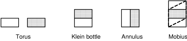
Figure 6: World sheets of short strings

Here the white (shaded) box represents the world sheet for the left (resp. right) mover. In the torus world sheets, the left and the right movers are independent and are detached from each other. In the Klein bottle, two boxes are piled vertically because of the orientation projection in the trace. In the annulus, they are piled horizontally because of the reflections at the boundaries. In the Möbius strip, they are piled horizontally and vertical at the same time. The fundamental parallelogram of Figure 4 is drawn by dashed line.

In the torus case discussed in section 2.2.2, we first introduce infinite plane with lattice points. We then assign the name of each short string to each rectangle by the rule determined from $h$ and $g$. In the open case, we need to put the left and right movers in the same plane. In the Klein bottle amplitude, there are toggles between left/right movers in the vertical direction (horizontal stripes). In the annulus, we have the toggling in the horizontal direction (vertical stripes). In the Möbius case, we have the toggling in both direction (checker board). We then put the names of the short string on each rectangle by using rule from $g$, $h$, and $f$ and determine the “fundamental region”. In the following, we will not try to exhaust all combinations appearing in the table. Rather we will illustrate the simple situation which will illuminate the topology change between the world sheets of the short and the long strings.

Klein bottle

In this case, there is toggling between torus/Klein bottle amplitude when viewed as the long string diagram. We explain it by taking the simplest situations $n=1$ and $m=2,3$.

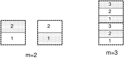
Figure 7: Klein bottles for short strings

In these cases, the left (resp. right) mover of $I+1$’th short string world sheet should be piled over the right (resp. left) mover of $I$’th. When $m=2$, we have independent two vertical loops, $L1\rightarrow R2\rightarrow L1$, $R1\rightarrow L2\rightarrow R1$ where $LI$ ($RI$) means the world sheet of the left (resp. right) mover of $I$’th short string. As we illustrate it in Figure 7 left, we have two independent rectangles of size 2. From the viewpoint of the long string, they should be identified as the left and right moving sectors of the long string. It is easy to observe that the similar phenomena occurs whenever $m$ is even.

If $m=3$, the six boxes should be attached with each other to form one big rectangle. It should be identified as the Klein bottle world sheet of the long string. It is easily generalized that the fat Klein bottle type world sheet appear whenever $m$ is odd.

Toggling between Annulus/Möbius strip long string amplitudes in the $I_{M}$ sector can be similarly understood.

Annulus

We first explain the appearance of the long open and closed strings by taking the simplest example which consists of two short strings in annulus diagram. We have two choices for $f_{1}$ and $f_{2}$, (A) $f_{1}=(1)(2)$, $f_{2}=(12)$ (B) $f_{1}=f_{2}=(12)$.

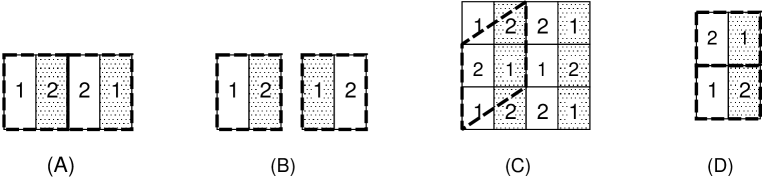
Figure 8: Annulus of short strings

In the first case, the horizontal attachments are defined as in Figure 8 (A) and we have only one chiral world sheet. This is the situation which describes annulus diagram for the long string. In the second case, we have two independent groups which are not attached each other Figure 8 (B). This is again the torus world sheet for the long string. We therefore meet the world sheet of the long closed string.

This is not the end of the story. Even in such a simple situation, we have a degree of freedom of the twist in the vertical direction. Since we are considering the annulus diagram, the world sheet of the left (right) mover should be piled vertically over that of the left (right) mover. Since we have two boxes for each, we have two choices for $g$, $g=1$ and $g=(12)$. In the first case, the diagrams is Figure 8(A,B) themselves. On the other hand, if we take $g=(12)$, we get two new world sheets (C,D). In diagram (C), as we draw a dashed line, the obtained diagram should be interpreted as the Möbius strip for the long string. For the diagram (D), two independent rectangles in (B) are piled vertically and gives the Klein bottle world sheet for the long string. In the table, (A) and (C) are classified as $I_{A}$ with $n=2$, $m=1$. (B) and (D) are classified as $\widetilde{II}_{A}$ and $II_{A}$ respectively with $n=1$ and $m=2$.

In this way, we get all the four diagrams of the long string amplitude from the annulus of the short string.

Möbius strip

In this case, we have the toggling of left and right movers in both horizontal and vertical directions. As in the annulus case, we explain the essence of the correspondence by using two short strip configurations. In figure 9, we illustrate three possible configurations.

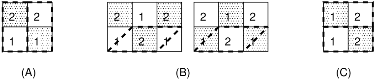
Figure 9: Möbius strip of short strings

The first one (A) corresponds to $I_{M}$ case ($n=1,m=2$) with $f_{1}=(1)(2)$, $g=(12)$. Because $m$ is even, we get the world sheet of annulus diagram. The second one corresponds to $II_{M}$ ($n=1,m=2$) with $f_{1}=g=(12)$. As illustrated in the figure (B), we have two independent parallelogram region with a twist by one block. It corresponds to the torus amplitude with $\tau_{1,1,1/2}$. The appearance of the half an odd integer is the characteristic feature in $II_{M}$ case. The third one corresponds to $\widetilde{II}_{M}$ case with $f_{1}=(12)$, $g=(1)(2)$. As depicted in the figure (C), it describes the world sheet of the Klein bottle

6 Boundary states

In this section, we show that there are basically two types of the boundary/cross-cap states in the symmetric product orbifold.

The first one is the conventional boundary/cross-cap states of the long string. One non-trivial point is that the boundary state for the short string ${|\,B:g,f\rangle\!\rangle}$ sometimes describes the cross-cap state of the long string. This is one of the origin of the change of the world sheet topology in the long string.

The second one describes the joint of two short strings. It helps to organize arbitrary long string world sheet from that of the short strings. This is clearly needed if our orbifold CFT has the character of the second quantized string theory. We will call such state as the joint state.

In usual description of the string theory, the boundary state describes the dynamics of the D-brane. In our approach, it is naturally unified into the interaction of the string fields.

6.1 Boundary states of short strings

Let us first derive the boundary states for the irreducible sets. Here we use the terminology “irreducible” to mean that it can not written as the direct product of the boundary states for the subset fields.

Let us start from a generic irreducible combination which satisfies $[g,f]=0$,

$$g=diag(\overbrace{{\overline{\cal T}}_{{\overline{n}}},\cdots,{\overline{\cal T}}_{{\overline{n}}}}^{\overline{m}})\,\,,\qquad f=diag({\overline{\cal T}}_{\overline{n}}^{{\overline{p}}_{0}},\cdots,{\overline{\cal T}}_{\overline{n}}^{{\overline{p}}_{{\overline{m}}-1}})\cdot{\cal T}_{\overline{m}}\,\,.$$ (6.1)

The condition $f^{2}=1$ firstly imposes the condition ${\overline{m}}=1,2$. When ${\overline{m}}=1$ (i.e. $f={\overline{\cal T}}_{\overline{n}}^{{\overline{p}}_{0}}$), $f^{2}=1$ implies $2{\overline{p}}_{0}\equiv 0$ mod ${\overline{n}}$. If ${\overline{n}}$ is odd, the only solution is ${\overline{m}}\equiv 0$ mod ${\overline{n}}$. If ${\overline{n}}$ is even, we have two solutions, ${\overline{m}}\equiv 0,{\overline{n}}/2$. When ${\overline{m}}=2$, $f^{2}=1$ is satisfied if ${\overline{p}}_{0}+{\overline{p}}_{1}\equiv 0$. We are left with only three types of the boundary states,

1. Boundary state of long string:   $(g,f)=({\overline{\cal T}}_{\overline{n}},1)$. If we use the mode expansion of the closed string (2.19) (while exchanging $n$ by ${\overline{n}}$), we get the explicit expression for the boundary state,

   $${|\,B:{\overline{\cal T}}_{n},1\rangle\!\rangle}=\exp\left(-\sum_{r=1}^{\infty}\sum_{a=0}^{{\overline{n}}-1}\frac{1}{r-a/{\overline{n}}}\alpha^{(a)}_{-r+a/{\overline{n}}}\tilde{\alpha}^{({\overline{n}}-a)}_{-r+a/{\overline{n}}}\right)|0\rangle_{\overline{n}}.$$ (6.2)

   We introduce the long string oscillator of length ${\overline{n}}$ as

   $${\cal A}_{{\overline{n}}p-a}\equiv\sqrt{{\overline{n}}}\alpha^{(a)}_{p-a/{\overline{n}}}\,\,,\qquad\widetilde{\cal A}_{{\overline{n}}p-a}\equiv\sqrt{{\overline{n}}}\tilde{\alpha}^{({\overline{n}}-a)}_{p-a/{\overline{n}}}.$$ (6.3)

   They satisfy a standard commutation relation $\left[{\cal A}_{n},{\cal A}_{m}\right]=n\delta_{n+m,0}$. The commutation relation with Hamiltonian is modified to $\left[L_{0},{\cal A}_{r}\right]=-\frac{r}{{\overline{n}}}{\cal A}_{r}$. In terms of this variable, the boundary state is rewritten as

   $$\exp\left(-\sum_{r=1}^{\infty}\frac{1}{r}{\cal A}_{-r}\widetilde{\cal A}_{-r}\right)|0\rangle_{\overline{n}}\equiv|B\rangle_{\overline{n}}\,\,.$$ (6.4)

   As for the zero mode, since we are considering the Neumann type boundary condition, we need to impose (writing $P$ for the momentum for ${\cal A}$)

   $$P|0\rangle_{\overline{n}}=0\,\,.$$ (6.5)

   This is nothing but the standard expression of the boundary state. We will denote the vacuum state for the $J$’s long oscillator satisfying (6.5) as $|0_{(J)}\rangle_{\overline{n}}$ in the following.

2. Cross-cap state for long string:   $(g,f)=({\overline{\cal T}}_{{\overline{n}}},{\overline{\cal T}}_{{\overline{n}}}^{{\overline{n}}/2})$
   This state exist only when ${\overline{n}}$ is even. (3.10) is satisfied by

   $${|\,B:{\overline{\cal T}}_{{\overline{n}}},{\overline{\cal T}}_{{\overline{n}}}^{{\overline{n}}/2}\rangle\!\rangle} \equiv |C\rangle_{\overline{n}}$$ (6.6)

   $$= \exp\left(-\sum_{r=1}^{\infty}\sum_{a=0}^{{\overline{n}}-1}\frac{(-1)^{a}}{r-a/{\overline{n}}}\alpha^{(a)}_{-r+a/{\overline{n}}}\tilde{\alpha}^{({\overline{n}}-a)}_{-r+a/{\overline{n}}}\right)|0\rangle_{\overline{n}}$$

   $$= \exp\left(-\sum_{r=1}^{\infty}(-1)^{r}\frac{1}{r}{\cal A}_{-r}\widetilde{\cal A}_{-r}\right)|0\rangle_{\overline{n}}\,\,.$$

   This is again the standard expression for the cross-cap state of the long string. This is the origin of the mixture of annulus/Möbius amplitude which we have observed in the previous section.

3. Joint state:

   $$g=\left(\begin{array}[]{c c}{\overline{\cal T}}_{\overline{n}}&0\\ 0&{\overline{\cal T}}_{\overline{n}}\end{array}\right)\,\,,\qquad f=\left(\begin{array}[]{c c}0&{\overline{\cal T}}_{\overline{n}}^{{\overline{p}}}\\ {\overline{\cal T}}_{\overline{n}}^{-{\overline{p}}}&0\end{array}\right)\,\,.$$ (6.7)

   This boundary state actually interconnects two long strings at the boundary. The boundary condition (3.10) can be easily solved to give,

   $${|\,B:g,f\rangle\!\rangle} \equiv |J\,(12),{\overline{p}}\rangle_{\overline{n}}$$

   $$= \exp\left(\sum_{r=1}^{\infty}\sum_{a=0}^{{\overline{n}}-1}\frac{1}{r-a/{\overline{n}}}\left({\bf e}\!\left[\frac{a{\overline{p}}}{{\overline{n}}}\right]\alpha^{(a,1)}_{-r+a/{\overline{n}}}\tilde{\alpha}^{({\overline{n}}-a,2)}_{-r+a/{\overline{n}}}\right.\right.$$

   $$\left.\left.+{\bf e}\!\left[\frac{-a{\overline{p}}}{{\overline{n}}}\right]\alpha^{(a,2)}_{-r+a/{\overline{n}}}\tilde{\alpha}^{({\overline{n}}-a,1)}_{-r+a/{\overline{n}}}\right)\right)|0\rangle_{\overline{n}}$$

   $$= \exp\left(\sum_{r=1}^{\infty}\frac{1}{r}\left({\bf e}\!\left[\frac{r{\overline{p}}}{{\overline{n}}}\right]{\cal A}^{(1)}_{-r}\widetilde{\cal A}^{(2)}_{-r}+{\bf e}\!\left[\frac{-r{\overline{p}}}{{\overline{n}}}\right]{\cal A}^{(1)}_{-r}\widetilde{\cal A}^{(2)}_{-r}\right)\right)|0\rangle_{\overline{n}}\,\,,$$

   where ${\cal A}^{(I)}$ ($I=1,2$) represents two long string variables.

As for the zero mode, the constraint from Dirichlet type boundary condition is written in terms of the zero mode as,

$$(x_{0}^{1}-x_{0}^{2})|0\rangle_{\overline{n}}=(P^{1}+P^{2})|0\rangle_{\overline{n}}=0\,\,.$$ (6.9)

We will denote the vacuum state which satisfy above condition for $I$th and $J$th long string as $|0_{(IJ)}\rangle$.

6.2 Cross-cap states of short strings

In the cross-cap states, $g$ and $f$ satisfies $f^{2}=g$. Since $\left[g,f\right]=\left[f^{2},f\right]=0$, $g$ and $f$ should be written in the form (6.1). As in the previous subsection, the constraint $f^{2}=g$ implies ${\overline{\cal T}}_{\overline{m}}^{2}=1$. So the only possibility is ${\overline{m}}=1,2$.

When ${\overline{m}}=1$, $f={\overline{\cal T}}^{\overline{p}}$ and $f^{2}=g$ gives $2{\overline{p}}\equiv 1$ mod ${\overline{n}}$. If ${\overline{n}}$ is odd, we have one solution ${\overline{p}}=({\overline{n}}+1)/2$. On the other hand if ${\overline{n}}$ is even we have no solution. When ${\overline{m}}=2$, the general solution to $f^{2}=g$ is (6.1) with $p_{0}+p_{1}\equiv 1$ mod $n$. We end up with two class of solutions,

1. Cross-cap states of the long string: $g={\overline{\cal T}}_{\overline{n}}$ and $f={\overline{\cal T}}_{\overline{n}}^{({\overline{n}}+1)/2}$ for odd ${\overline{n}}$.
   In this case one may reshuffle the basis to write $f={\overline{\cal T}}_{\overline{n}}$ and $g={\overline{\cal T}}_{\overline{n}}^{2}$. The mode expansion (2.19) is slightly modified to

   $$\widetilde{\bf X}^{a}=\alpha_{0}\delta_{a,0}\sigma_{0}+i\sum_{r\in{\bf Z}}\left(\frac{1}{r-2a/{\overline{n}}}\alpha^{a}_{r-2a/{\overline{n}}}z^{-r+2a/{\overline{n}}}+\frac{1}{r+2a/{\overline{n}}}\tilde{\alpha}^{a}_{r+2a/{\overline{n}}}\bar{z}^{-r-2a/{\overline{n}}}\right)$$ (6.10)

   The boundary condition (3.28) can be written in terms of oscillators as

   $$(\alpha^{a}_{r-2a/{\overline{n}}}+(-1)^{r}\tilde{\alpha}^{{\overline{n}}-a}_{-r+2a/{\overline{n}}}){|\,C:f^{2},f\rangle\!\rangle}=0\,\,,$$ (6.11)

   where the twist factor $f$ (3.28) is exactly canceled by the translation of $\sigma_{1}$. Now it is straightforward to write down the cross-cap state,

   $${|\,C:{\overline{\cal T}}_{{\overline{n}}}^{2},{\overline{\cal T}}_{{\overline{n}}}\rangle\!\rangle}=\exp\left(-\sum_{r=1}^{\infty}\sum_{a=0}^{{\overline{n}}-1}\frac{(-1)^{r}}{r-2a/{\overline{n}}}\alpha^{(a)}_{-r+2a/{\overline{n}}}\tilde{\alpha}^{({\overline{n}}-a)}_{-r+2a/{\overline{n}}}\right)|0\rangle_{\overline{n}}\\$$

   It is not difficult from this point to show that after redefinition of the long string variable, it reduces to (6.6).

2. Joint state:

   $$g=\left(\begin{array}[]{c c}{\overline{\cal T}}_{\overline{n}}&0\\ 0&{\overline{\cal T}}_{\overline{n}}\end{array}\right)\,\,,\qquad f=\left(\begin{array}[]{c c}0&{\overline{\cal T}}_{\overline{n}}^{{\overline{p}}+1}\\ {\overline{\cal T}}_{\overline{n}}^{-{\overline{p}}}&0\end{array}\right)\,\,.$$ (6.12)

   After repeating the similar calculation, we arrive at (3) with ${\overline{p}}$ replaced by ${\overline{p}}+1/2$. Clearly this is the origin of half-twist which appeared in the fat torus amplitude (5.34).

In either cases, the condition for the zero-mode are the same as in the boundary states (6.5,6.9).

6.3 Inner product between boundary states

In this subsection, we calculate the inner product between boundary states of the short strings to see the modular property of the long open strings. In the following, we will restrict our attraction to the boundary states since the calculation of the cross-cap states are completely analogous.

In order to reproduce the open string amplitudes from the boundary state, we need to loosen the the irreducibility of the boundary state. We therefore start from the general form (6.1) and impose the condition $f^{2}=1$.

The general solution is given by

$$f=diag({\overline{\cal T}}^{{\overline{p}}_{0}}_{\overline{n}},\cdots,{\overline{\cal T}}_{\overline{n}}^{{\overline{p}}_{{\overline{m}}-1}})\cdot{\cal T}_{{\overline{m}}}^{q}{\cal S}_{\overline{m}}\,\,.$$ (6.13)

The constraint $f^{2}=1$ further imposes

$${\overline{p}}_{\ell}+{\overline{p}}_{{\overline{m}}-1-\ell+q}\equiv 0\quad\mbox{mod}\,\,{\overline{n}}\,\,.$$ (6.14)

The corresponding boundary state ${|\,B:g,f\rangle\!\rangle}$ can be decomposed into the product of the (long string) boundary, cross-cap, and joint states. When

$$\ell\equiv{\overline{m}}-1-\ell+q\qquad\mbox{ mod}\,\,{\overline{m}}\,\,,$$ (6.15)

it is described by the boundary and cross-cap states and otherwise it is given by the joint state. Let us first count the number of the boundary and cross-cap states.

Figure 10: Loose ends of long string

We remark first that ${\overline{m}}$ is the number of long open strings which have their open end at the boundary. When ${\overline{m}}$ is even and $q$ is odd, we have two solutions to (6.15), $\ell=(q-1)/2,(q-1+{\overline{m}})/2$. In this case, the long string has two loose end at that boundary and the others are connected each other (Figure 10 left). When ${\overline{m}}$ is even and $q$ is even, we have no solution and every long strings are jointed each other. On the other hand, when ${\overline{m}}$ is odd, we always have only one loose end (Figure 10 right).

6.3.1 Annulus/Möbius strip/Klein bottle amplitudes

Let us assume that $f_{1}$ and $f_{2}$ (reflection factors at each boundary) to have the general form (6.13)

$$f_{1}=diag({\overline{\cal T}}^{{\overline{p}}^{(1)}_{0}}_{\overline{n}},\cdots,{\overline{\cal T}}_{\overline{n}}^{{\overline{p}}^{(1)}_{{\overline{m}}-1}})\cdot{\cal T}_{{\overline{m}}}^{q_{1}}{\cal S}_{\overline{m}}\,\,,\quad f_{2}=diag({\overline{\cal T}}^{{\overline{p}}^{(2)}_{0}}_{\overline{n}},\cdots,{\overline{\cal T}}_{\overline{n}}^{{\overline{p}}^{(2)}_{{\overline{m}}-1}})\cdot{\cal T}_{{\overline{m}}}^{q_{2}}{\cal S}_{\overline{m}}\,\,.$$ (6.16)

Annulus, Möbius strip and Klein bottle amplitudes can be obtained if there are two loose ends at the boundaries. Such situations can be obtained if (i) ${\overline{m}}$ is odd, or (ii) ${\overline{m}}$ is even and $q_{1}-q_{2}$ is odd. To get the irreducible diagram, one may always obtain a basis where $q_{1}=1$ and $q_{2}=0$ in either cases.

In the explicit evaluation, we use the following formula,

$$\langle 0|e^{-f_{2}^{IJ}\alpha_{I}\tilde{\alpha}_{J}q}e^{-f_{1}^{KL}\alpha^{\dagger}_{K}\tilde{\alpha}^{\dagger}_{L}}|0\rangle=\prod_{a}\frac{1}{1-\mu_{a}q}\,\,,$$ (6.17)

where oscillators satisfy the commutation relations $\left[\alpha_{I},\alpha^{\dagger}_{J}\right]=\left[\tilde{\alpha}_{I},\tilde{\alpha}^{\dagger}_{J}\right]=\delta_{IJ}$ and $\mu_{a}$ are the eigenvalues of $f_{2}f_{1}^{t}$.

In our case, $f_{2}\,f_{1}^{t}=f_{2}\,f_{1}$ is given by

$$diag({\overline{\cal T}}_{\overline{n}}^{{\overline{p}}_{0}^{(2)}+{\overline{p}}_{{\overline{m}}-1}^{(1)}},{\overline{\cal T}}_{\overline{n}}^{{\overline{p}}_{1}^{(2)}+{\overline{p}}_{{\overline{m}}-2}^{(1)}},\cdots)\cdot{\cal T}_{{\overline{m}}}^{-1}.$$ (6.18)

As we have been doing in section 2, we first diagonalize the ${\overline{\cal T}}_{\overline{n}}$ action by discrete Fourier transformation. In the subspace where ${\overline{\cal T}}_{\overline{n}}\cdot{\bf X}^{a,J}={\bf e}\!\left[\frac{a}{{\overline{n}}}\right]{\bf X}^{a,J}$, the eigenvalues of this matrix should satisfy

$$\mu^{\overline{m}}={\bf e}\!\left[\frac{a}{{\overline{n}}}\left(\sum_{\ell=0}^{{\overline{m}}-1}({\overline{p}}^{(2)}_{\ell}+{\overline{p}}^{(1)}_{{\overline{m}}-1-\ell})\right)\right]$$ (6.19)

Because of (6.14), almost all the terms except for ${\overline{p}}$ at the loose ends cancel each other in the right hand side. For the annulus/Klein bottle amplitude, the phase at the loose end cancel each other and $\mu^{\overline{m}}=1$. For the Möbius strip amplitude, we have non-trivial phase $\mu^{\overline{m}}=(-1)^{a}$ since $\sum{\overline{p}}={\overline{n}}/2$.

For the oscillator contribution of the annulus and Klein bottle amplitude, we obtain the inner product as,

$${\langle\!\langle B:g,f_{2}\,|}q^{L_{0}+\bar{L}_{0}}{|\,B:g,f_{1}\rangle\!\rangle}^{oscillator} = \prod_{r=1}^{\infty}\prod_{a=0}^{{\overline{n}}-1}\prod_{b=0}^{{\overline{m}}-1}\frac{1}{1-{\bf e}\!\left[b/{\overline{m}}\right]q^{2(r-a/{\overline{n}})}}$$ (6.20)

$$= \prod_{r=1}^{\infty}\frac{1}{1-q^{2{\overline{m}}r/{\overline{n}}}}$$

Similarly for the Möbius strip amplitude (${\overline{n}}$ should be even in this case),

$${\langle\!\langle B:g,f_{2}\,|}q^{L_{0}+\bar{L}_{0}}{|\,B:g,f_{1}\rangle\!\rangle}^{oscillator} = \prod_{r=1}^{\infty}\prod_{a=0}^{{\overline{n}}-1}\prod_{b=0}^{{\overline{m}}-1}\frac{1}{1-{\bf e}\!\left[\frac{b}{{\overline{m}}}+\frac{a}{2{\overline{m}}}\right]q^{2(r-a/{\overline{n}})}}$$ (6.21)

$$= \prod_{r=1}^{\infty}\frac{1}{1-(-1)^{r}q^{2{\overline{m}}r/{\overline{n}}}}$$

For the zero mode contribution to the inner product, we use the momentum representation of the vacuum states,

$$\langle P^{I}|0_{(I)}\rangle_{\overline{n}}=\delta(P^{I}),\qquad\langle P^{I},P^{J}|0_{(IJ)}\rangle_{\overline{n}}=\delta(P^{I}+P^{J}).$$ (6.22)

If ${\overline{m}}$ is even, the inner product can be written in the following form,

$${}_{\overline{n}}\langle 0_{(1)(23)\cdots({\overline{m}}-2,{\overline{m}}-1)({\overline{m}})}|q^{\frac{1}{2{\overline{n}}}(L_{0}+\bar{L}_{0})}|0_{(12)\cdots({\overline{m}}-1,{\overline{m}})}\rangle_{\overline{n}}$$

$$\qquad=\int d^{\overline{m}}P\,\,{}_{\overline{n}}\langle 0_{(1)(23)\cdots({\overline{m}}-2,{\overline{m}}-1)({\overline{m}})}|\vec{P}\rangle q^{\frac{1}{2{\overline{n}}}\sum_{I}P_{I}^{2}}\langle\vec{P}|0_{(12)\cdots({\overline{m}}-1,{\overline{m}})}\rangle_{\overline{n}}$$

$$\qquad=\int d^{\overline{m}}P\,\,\delta(P_{1})\delta(P_{1}+P_{2})\delta(P_{2}+P_{3})\cdots\delta(P_{{\overline{m}}-1}+P_{\overline{m}})\delta(P_{\overline{m}})q^{\frac{1}{2{\overline{n}}}\sum_{I}P_{I}^{2}}$$

$$\qquad=\delta(0)=V.$$ (6.23)

Here $V$ is the volume and $|0_{(12)\cdots({\overline{m}}-1,{\overline{m}})}\rangle_{\overline{n}}$ is the short hand notation of $|0_{(12)}\rangle_{\overline{n}}\otimes\cdots\otimes|0_{{\overline{m}}-1,{\overline{m}}}\rangle_{\overline{n}}$. Calculation for odd ${\overline{m}}$ is mostly the same and gives the same answer.

6.3.2 Torus

In order to get the torus amplitude, ${\overline{m}}$ should be even since the both boundary should have no loose ends. Similarly both $q_{1}$ and $q_{2}$ are even to fulfill this relation. In order to get the irreducible amplitude, one may put $q_{1}=2$ and $q_{2}=0$ without losing generality. In this case $f_{2}f_{1}$ is given by

$$diag({\overline{\cal T}}_{\overline{n}}^{{\overline{p}}_{0}^{(2)}+{\overline{p}}_{{\overline{m}}-1}^{(1)}},{\overline{\cal T}}_{\overline{n}}^{{\overline{p}}_{1}^{(2)}+{\overline{p}}_{{\overline{m}}-2}^{(1)}},\ldots)\cdot{\cal T}_{{\overline{m}}}^{-2}.$$ (6.24)

Since ${\overline{m}}$ is even, we have two sets of eigenvalue equations,

$$\mu^{{\overline{m}}/2}={\bf e}\!\left[\pm\frac{a{\overline{p}}}{{\overline{n}}}\right],\quad{\overline{p}}\equiv\sum_{\ell=0}^{{\overline{m}}/2-1}({\overline{p}}^{(2)}_{2\ell}+{\overline{p}}^{(1)}_{{\overline{m}}-1-2\ell})\,\,.$$ (6.25)

Unlike the situation in the previous subsection, ${\overline{p}}$ can take any integer.

Writing $k={\overline{m}}/2$, we obtain the oscillator part of the torus amplitude,

$${\langle\!\langle B:g,f_{2}\,|}q^{L_{0}+\bar{L}_{0}}{|\,B:g,f_{1}\rangle\!\rangle}^{oscillator}$$

$$\qquad=\prod_{r=1}^{\infty}\prod_{a=0}^{{\overline{n}}-1}\prod_{b=0}^{k-1}\frac{1}{(1-{\bf e}\!\left[\frac{b}{{\overline{k}}}+\frac{a{\overline{p}}}{{\overline{k}}}\right]q^{2(r-a/{\overline{n}})})(1-{\bf e}\!\left[\frac{b}{{\overline{k}}}-\frac{a{\overline{p}}}{{\overline{k}}}\right]q^{2(r-a/{\overline{n}})})}$$

$$\qquad=\prod_{r=1}^{\infty}\frac{1}{(1-{\bf e}\!\left[\frac{2{\overline{k}}\tau+{\overline{p}}}{{\overline{n}}}\right])(1-{\bf e}\!\left[\frac{2{\overline{k}}\tau-{\overline{p}}}{{\overline{n}}}\right])}$$ (6.26)

For the zero mode calculation, the calculation is parallel to (6.23). The only difference is the product of the delta functions of $P$. The integral produces,

$$\int d^{\overline{m}}P\,\,\delta(P_{1}+P_{2})\delta(P_{2}+P_{3})\cdots\delta(P_{{\overline{m}}-1}+P_{\overline{m}})\delta(P_{{\overline{m}}}+P_{1})q^{\frac{1}{2{\overline{n}}}\sum_{I}P_{I}^{2}}$$

$$\qquad=\delta(0)\int dPq^{\frac{{\overline{m}}}{2{\overline{n}}}P^{2}}=V(\mbox{Im}\,\tau_{{\overline{n}},{\overline{m}},0})^{-1/2}\,\,.$$ (6.27)

The moduli dependence appearing here is necessary to have the correct modular property.

7 DLCQ partition function

In this section, we prove that the various amplitudes of the open string are organized to give the simple formula similar to (2.54). Such a structure is needed to identify our model as the DLCQ of the open string field theory as we reviewed in section 2.3.

Unlike the closed string partition function, the requirement of the modular invariance does not necessarily determine the combinations of the twisted open string sectors (3.4, 3.14). It is quite encouraging that the summation over the all possible twists indeed gives the DLCQ type partition function.

Usually in BCFT, the combination of various sectors is determined by the tadpole cancellation condition. In terms of the boundary state and the cross cap state, it is written as the cancellation of the massless part of the boundary states,

$$|B\rangle\!\rangle_{0}+|C\rangle\!\rangle_{0}=0\,\,.$$ (7.1)

In the bosonic string in the flat target space, this condition determine the gauge group should be $SO(2^{13})$. In other situations, this gives a crucial constraint on the model building. While we try to apply the tadpole condition (7.1) naively, we meet one difficulty. Namely the generic one loop amplitude is reducible and its irreducible components have a tachyonic part. Multiplying them usually produces the higher negative modes which complicate the constraint (7.1). It usually becomes a nonlinear relation and the analysis would be very difficult. Such a situation will be remedied if we have the DLCQ type partition function. In this case, products of the various string amplitudes can be organized as the exponential of the sum of the irreducible ones. We can examine the tadpole condition for each of the single long string amplitudes.

We will summarize our results in the following theorem,

Theorem 3 : (i) Klein bottle:
The generating function of the partition function,

$$Z^{KB}_{N}(\tau)=\frac{1}{N!}\sum_{g,h\in S_{N}}\mbox{Tr}_{{\cal H}_{h}}(g\Omega^{closed}{\bf e}\!\left[\tau(L_{0}+\bar{L}_{0})\right]),$$ (7.2)

with a constraint $hg=gh^{-1}$, is written as

$$\ln(\sum_{N=0}^{\infty}\zeta^{N}Z_{N}^{KB}(\tau))$$ (7.3)

$$\quad=\sum_{n,m=1}^{\infty}\left(\frac{\zeta^{n(2m-1)}}{2m-1}{\cal Z}^{KB}(\tau_{n,2m-1})+\frac{\zeta^{2nm}}{2nm}\sum_{p=0}^{n-1}{\cal Z}^{Torus}(\tau_{n,2m,p},\bar{\tau}_{n,2m,p})\right).$$

(ii) Annulus :
The generating function of the partition function,

$$Z_{N}^{Annulus}=\frac{1}{N!}\sum_{h,g,f_{1},f_{2}\in S_{N}}\mbox{Tr}_{{\cal H}_{f_{1},f_{2}}}\left(g\,{\bf e}\!\left[\tau L_{0}\right]\right)\,\,,$$ (7.4)

with the constraint, $\left[g,f_{1}\right]=\left[g,f_{2}\right]=0$, $f_{1}^{2}=f_{2}^{2}=1$, $h=f_{2}^{-1}f_{1}$ is written in the following form,

$$\ln(\sum_{N=0}^{\infty}\zeta^{N}Z_{N}^{Annulus}(\tau))$$

$$\quad=\sum_{n,m=1}^{\infty}\frac{\zeta^{nm}}{m}{\cal Z}^{Annulus}(\tau_{n,m,0})+\sum_{n,m=1}^{\infty}\frac{\zeta^{2nm}}{m}{\cal Z}^{Mobius}(\tau_{2n,m,0})$$

$$\quad+\sum_{n,m=1}^{\infty}\frac{\zeta^{2nm}}{2nm}\sum_{p=0}^{n-1}{\cal Z}^{Torus}(\tau_{n,m,p},\bar{\tau}_{n,m,p})+\sum_{n,m=1}^{\infty}\frac{\zeta^{2nm}}{2m}{\cal Z}^{KB}(\tau_{n,m,0}).$$

(iii) Möbius strip :
The generating function of the partition function,

$$Z_{N}^{Mobius}=\frac{1}{N!}\sum_{h,g,f\in S_{N}}\mbox{Tr}_{{\cal H}_{f,gfg^{-1}}}\left(g\Omega^{open}\,{\bf e}\!\left[\tau L_{0}\right]\right)\,\,,$$ (7.6)

with the constraint, $h=gfg^{-1}f$, $f^{2}=1$, $\left[g^{2},f\right]=0$, is given as follows,

$$\ln(\sum_{N=0}^{\infty}\zeta^{N}Z_{N}^{Mobius}(\tau))$$

$$\quad=\sum_{n,m=1}^{\infty}\frac{\zeta^{2nm}}{2m}{\cal Z}^{Annulus}(\tau_{n,2m,0})+\sum_{n,m=1}^{\infty}\frac{\zeta^{(2n-1)m}}{m}{\cal Z}^{Mobius}(\tau_{2n-1,m,0})$$ (7.7)

$$\quad+\sum_{n,m=1}^{\infty}\frac{\zeta^{2nm}}{2nm}\sum_{p=0}^{n-1}{\cal Z}^{Torus}(\tau_{n,m,p+n/2},\bar{\tau}_{n,2m,p+n/2})+\sum_{n,m=1}^{\infty}\frac{\zeta^{2nm}}{2m}{\cal Z}^{KB}(\tau_{n,m,0}).$$

Proof:
Klein bottle: The strategy is completely parallel to our discussion in section 2.2.3. We first choose an element $h$ which represents each conjugacy class. For each $h$, we need to count the number of the elements $g$ which satisfies this constraint. By comparing (2.2.1) and (4.1), we have the same degree of freedom for $g$ including the introduction of parameter $p$. The only deference is that the Klein bottle amplitude at the end does not depend on $p$. Therefore the summation $\frac{1}{n}\sum_{p}$ does not exist. We can conclude that it has the same type of the generating functional (7.3). Annulus and Möbius strip:
We have three class of solutions (• ‣ 4,• ‣ 4,4.6). For given $N$, the annulus partition function is the sum of the products of all possible combinations of three irreducible solutions. If we combine them into the generating function, the contributions from each diagram are factorized and we can count them independently. Although we have extra summation over $f_{i}$, the number of the solutions are almost the same if we look at (• ‣ 4,• ‣ 4,4.6) carefully.

For type $I_{A}$ solutions, there are one constraint on $p$, $2\sum_{\ell}p_{\ell}\equiv 0$. For each value of $\sum_{\ell}p_{\ell}$, we have $n$ solutions for $q$ which satisfies (4.3). Since the final expression (5.22) does not depend on $q$, we have the same number of degree of freedom as in the torus case. This type of counting holds exactly the same fashion for type $II_{A}$ solutions.

For type $\widetilde{II}_{A}$, we need to be more careful to count the combinations. However, the final expression turns out to be the same as in $II_{A}$ case.

By combining all types of the solutions, we arrive at (7).

The calculation of the combinatorics is exactly the same for the Möbius strip case. QED

8 Tadpole Condition

In the previous section, we have seen that four sectors (Torus, Klein bottle, Annulus, Möbius strip) of the long string are actually contained in the annulus diagram of the short open string. This leads us to suspect that we may accomplish the tadpole condition (7.1) by combining the boundary states of the short strings. One subtle issue is that there is no cross-cap state when ${\overline{n}}$ is odd (it is described as the cross-cap state of the short string). In order to achieve the tadpole condition in terms of boundary states alone, we need to restrict the length of the long strings (${\overline{n}}$) to be even. This condition may be imposed by setting normalization factor for those boundary states is zero.

In the following, we will restrict our discussion to the tadpole cancellation between various amplitudes for the single long string. It is not necessarily equivalent to the tadpole condition in conventional BCFT [44]–[45]. Usually the tadpole condition is used to derive consistent compactification of the target space. In our case, however, the symmetric product is used to describe the string field theory. We believe that the our treatment is the appropriate one in this physically different context.

Before we start the discussion, we should comment on the dimension of the target space. In the following we will discuss on the standard bosonic string. In order to recover the Lorentz covariance, we need put the transverse dimension of the target space to be 24. The change of the various amplitude is straightforward.

As was seen in section 6.3, the boundary and cross-cap states of long strings are constructed by the products of irreducible boundary, cross-cap and joint states. The normalizations of these states should be also factorized into those of each irreducible boundary states. We will denote them as $\kappa_{B},\kappa_{C}$ and $\kappa_{J}$. The structure of the boundary and cross-cap states of the long strings are slightly different if ${\overline{m}}$ is even or ${\overline{m}}$ is odd.

First, we will discuss odd ${\overline{m}}$ case (Figure 10 right). There is one loose end on each boundary. Long string boundary states are written as

$${|\,B:g,f^{B}\rangle\!\rangle}=\kappa_{J}^{({\overline{m}}-1)/2}\kappa_{B}\sum_{\left\{{\overline{p}}\right\}}(\prod_{i=1}^{({\overline{m}}-1)/2}|J(2i-1,2i),{\overline{p}}_{i}\rangle_{\overline{n}})\otimes|B\rangle_{\overline{n}}\,\,,$$ (8.1)

where $g=diag(\overbrace{{\overline{\cal T}}_{{\overline{n}}},\cdots,{\overline{\cal T}}_{{\overline{n}}}}^{\overline{m}})\,\,$. $f^{B}=diag({\overline{\cal T}}^{{\overline{p}}^{(B)}_{0}}_{\overline{n}},\cdots,{\overline{\cal T}}_{\overline{n}}^{{\overline{p}}^{(B)}_{{\overline{m}}-1}})\cdot{\cal T}_{{\overline{m}}}^{q_{B}}{\cal S}_{\overline{m}}\,$. It contains a loose end (boundary) on ${\overline{m}}$’th long string. Long string cross-cap states are written as

$${|\,B:g,f^{C}\rangle\!\rangle}=\kappa_{J}^{({\overline{m}}-1)/2}\kappa_{C}\sum_{\left\{{\overline{p}}\right\}}(\prod_{i=1}^{({\overline{m}}-1)/2}|J(2i-1,2i),{\overline{p}}_{i}\rangle_{\overline{n}})\otimes|C\rangle_{\overline{n}}\,\,,$$ (8.2)

where $f^{C}=diag({\overline{\cal T}}^{{\overline{p}}^{(C)}_{0}}_{\overline{n}},\cdots,{\overline{\cal T}}_{\overline{n}}^{{\overline{p}}^{(C)}_{{\overline{m}}-1}})\cdot{\cal T}_{{\overline{m}}}^{q_{C}}{\cal S}_{\overline{m}}\,\,$. It contains a cross-cap on ${\overline{m}}$’th long string.

Tadpole cancellation condition 7.1 is factorized into the following conditions,

$$\kappa_{B}|B\rangle_{{\overline{n}}0}\,\,+\kappa_{C}|C\rangle_{{\overline{n}}0}\,\,=0\,\,.$$ (8.3)

$$\sum_{{\overline{p}}_{i}}|J(2i-1,2i),{\overline{p}}_{i}\rangle_{{\overline{n}}0}=0\,\,.$$ (8.4)

The condition for the joint states (8.4) is satisfied automatically since,

$$\sum_{{\overline{p}}_{i}}|J(2i-1,2i),{\overline{p}}_{i}\rangle_{{\overline{n}}0}$$

$$\qquad=\left(\sum_{p}{\bf e}\!\left[p/{\overline{n}}\right]\right)({\cal A}^{(2i-1)}_{-r}\widetilde{\cal A}^{(2i)}_{-r}+{\cal A}^{(2i)}_{-r}\widetilde{\cal A}^{(2i-1)}_{-r})|0_{2i-1,2i}\rangle=0\,\,.$$ (8.5)

There are no constraints for $\kappa_{J}$. For the boundary and the cross-cap states, tadpole condition is satisfied when

$$\kappa_{B}-\kappa_{C}=0\,\,.$$ (8.6)

Let us move to even ${\overline{m}}$ case (Figure 10 left). There are two loose ends on one boundary and no loose ends on the other. The long string boundary states (written as ${|\,B:g,f^{J}\rangle\!\rangle}$) which does not have any loose ends, don’t make any contributions for the tadpole cancellation conditions since they are factorized into the joint states.

We introduce the long string boundary state for Annulus ${|\,B:g,f^{A}\rangle\!\rangle}$, Möbius strip ${|\,B:g,f^{MS}\rangle\!\rangle}$, and Klein bottle ${|\,B:g,f^{KB}\rangle\!\rangle}$ as follows,

$${|\,B:g,f^{A}\rangle\!\rangle} = \kappa_{J}^{({\overline{m}}-2)/2}\kappa_{B}^{2}(\prod_{i=1}^{{\overline{m}}/2-1}\sum_{{\overline{p}}^{i}}|J(2i,2i+1),{\overline{p}}_{i}\rangle_{\overline{n}})\otimes|B(1)\rangle_{\overline{n}}\,\,\otimes|B({\overline{m}})\rangle_{\overline{n}}\,\,,$$

$${|\,B:g,f^{MS}\rangle\!\rangle} = \kappa_{J}^{({\overline{m}}-2)/2}\kappa_{B}\kappa_{C}(\prod_{i=1}^{{\overline{m}}/2-1}\sum_{{\overline{p}}_{i}}|J(2i,2i+1),{\overline{p}}_{i}\rangle_{\overline{n}})$$ (8.7)

$$\qquad\otimes(|B(1)\rangle_{\overline{n}}\,\,\otimes|C({\overline{m}})\rangle_{\overline{n}}\,\,+|C(1)\rangle_{\overline{n}}\,\,\otimes|B({\overline{m}})\rangle_{\overline{n}}\,\,),$$

$${|\,B:g,f^{KB}\rangle\!\rangle} = \kappa_{J}^{({\overline{m}}-2)/2}\kappa_{C}^{2}(\prod_{i=1}^{{\overline{m}}/2-1}\sum_{{\overline{p}}_{i}}|J(2i,2i+1),{\overline{p}}_{i}\rangle_{\overline{n}})\otimes|C(1)\rangle_{\overline{n}}\,\,\otimes|C({\overline{m}})\rangle_{\overline{n}}\,\,.$$

The name of these states comes from the inner product formulae,

$$Z^{A} \sim {\langle\!\langle B:g,f^{J}\,|}q^{L_{0}+\bar{L_{0}}}{|\,B:g,f^{A}\rangle\!\rangle}\,\,,$$

$$Z^{M} \sim {\langle\!\langle B:g,f^{J}\,|}q^{L_{0}+\bar{L_{0}}}{|\,B:g,f^{MS}\rangle\!\rangle}\,\,,$$

$$Z^{KB} \sim {\langle\!\langle B:g,f^{J}\,|}q^{L_{0}+\bar{L_{0}}}{|\,B:g,f^{KB}\rangle\!\rangle}.$$ (8.8)

Tadpole cancellation condition (7.1) becomes

$${|\,B:g,f^{A}\rangle\!\rangle}_{0}+{|\,B:g,f^{MS}\rangle\!\rangle}_{0}+{|\,B:g,f^{KB}\rangle\!\rangle}_{0}$$

$$\qquad=\kappa_{J}^{({\overline{m}}-2)/2}((\prod_{i=1}^{{\overline{m}}/2-1}\sum_{{\overline{p}}_{i}}|J(2i,2i+1){\overline{p}}_{i}\rangle_{{\overline{n}}})$$ (8.9)

$$\left.\quad\qquad\otimes(\kappa_{B}|B(1)\rangle_{{\overline{n}}}\,\,+\kappa_{C}|C(1)\rangle_{{\overline{n}}})\otimes(\kappa_{B}|B({\overline{m}})\rangle_{{\overline{n}}}\,\,+\kappa_{C}|C({\overline{m}})\rangle_{{\overline{n}}})\right)_{0}=0\,\,.$$

Since it is factorized, it does not produce any new constraints on $\kappa$’s.

To determine Chan-Paton factor, we calculate the modular properties of various open string amplitudes. In section 6 we determine the inner products between various boundary states. Together with the normalization factors, annulus/Möbius strip/Klein bottle amplitudes with length ${\overline{m}}$ are given as (6.20, 6.21),

Annulus : $$({\overline{n}}\kappa_{J})^{{\overline{m}}-1}(\kappa_{B})^{2}{\bf e}\!\left[\frac{{\overline{m}}}{{\overline{n}}\tau}\right]\prod_{r=1}^{\infty}\left(1-{\bf e}\!\left[-\frac{{\overline{m}}}{{\overline{n}}\tau}r\right]\right)^{-24}\,\,,$$

Möbius : $$2({\overline{n}}\kappa_{J})^{{\overline{m}}-1}(\kappa_{B})^{2}{\bf e}\!\left[\frac{{\overline{m}}}{{\overline{n}}\tau}\right]\prod_{r=1}^{\infty}\left(1-(-1)^{r}{\bf e}\!\left[-\frac{{\overline{m}}}{{\overline{n}}\tau}r\right]\right)^{-24}\,\,$$

KB : $$({\overline{n}}\kappa_{J})^{{\overline{m}}-1}(\kappa_{B})^{2}{\bf e}\!\left[\frac{{\overline{m}}}{{\overline{n}}\tau}\right]\prod_{r=1}^{\infty}\left(1-{\bf e}\!\left[-\frac{{\overline{m}}}{{\overline{n}}\tau}r\right]\right)^{-24}\,\,.$$ (8.10)

To achieve the tadpole condition (8.3), we need to restrict ${\overline{n}}$ to be even. We will write ${\overline{n}}=2{\overline{k}}$ in the following.

After the modular transformation, these amplitudes are rewritten as,

Annulus : $$({\overline{n}}\kappa_{J})^{{\overline{m}}-1}(\kappa_{B})^{2}\left(\frac{2{\overline{k}}\tau}{i{\overline{m}}}\right)^{-12}{\bf e}\!\left[-\frac{2{\overline{k}}\tau}{{\overline{m}}}\right]\prod_{r=1}^{\infty}\left(1-{\bf e}\!\left[\frac{2{\overline{k}}\tau}{{\overline{m}}}r\right]\right)^{-24}\,\,,$$

Möbius : $$2({\overline{n}}\kappa_{J})^{{\overline{m}}-1}(\kappa_{B})^{2}\left(\frac{{\overline{k}}\tau}{i{\overline{m}}}\right)^{-12}{\bf e}\!\left[-\frac{{\overline{k}}\tau}{2{\overline{m}}}\right]\prod_{r=1}^{\infty}\left(1-(-1)^{r}{\bf e}\!\left[\frac{{\overline{k}}\tau}{2{\overline{m}}}r\right]\right)^{-24}\,\,,$$

KB : $$({\overline{n}}\kappa_{J})^{{\overline{m}}-1}(\kappa_{B})^{2}\left(\frac{2{\overline{k}}\tau}{i{\overline{m}}}\right)^{-12}{\bf e}\!\left[-\frac{2{\overline{k}}\tau}{{\overline{m}}}\right]\prod_{r=1}^{\infty}\left(1-{\bf e}\!\left[\frac{2{\overline{k}}\tau}{{\overline{m}}}r\right]\right)^{-24}\,\,.$$ (8.11)

These expression should be compared to the partition functions obtained in section 5.

Annulus : $$\frac{N^{2}}{4}\left(\frac{2m\tau}{in}\right)^{-12}{\bf e}\!\left[-\frac{m\tau}{n}\right]\prod_{r=1}^{\infty}\left(1-{\bf e}\!\left[\frac{m\tau}{n}r\right]\right)^{-24}\,\,,$$

Möbius : $$N\eta\left(\frac{m\tau}{ik}\right)^{-12}{\bf e}\!\left[-\frac{m\tau}{2k}\right]\prod_{r=1}^{\infty}\left(1-(-1)^{r}{\bf e}\!\left[\frac{m\tau}{2k}r\right]\right)^{-24}\,\,,$$

KB : $$\left(\frac{\tau k}{in}\right)^{-12}{\bf e}\!\left[-\frac{2k\tau}{n}\right]\prod_{r=1}^{\infty}\left(1-{\bf e}\!\left[\frac{2k\tau}{n}r\right]\right)^{-24}\,\,.$$ (8.12)

Here $N$ is the Chan-Paton factor for the long open strings and we write $m=2k$ in Möbius and KB amplitudes since they appear only when $m$ is even. By comparing expressions, we first need impose $\kappa_{J}={\overline{n}}^{-1}$ since there are no length dependent factors in (8). By comparing the oscillators, we need to impose,

• Annulus: $m=2{\overline{k}}$, $n={\overline{m}}$

• Möbius: $m={\overline{k}}$, $k={\overline{m}}$

• Klein bottle: $k={\overline{k}}$, $n={\overline{m}}$

It shows that we need to project to even $m$ sector for Annulus in (7) because the restriction that ${\overline{n}}$ is even. For other sectors, it reproduces every terms in (7). By comparing the normalization factor, we get

$$\frac{1}{4}N^{2}2^{-12} = (\kappa_{B})^{2}\,\,\,,$$

$$N\eta = 2(\kappa_{B})^{2}\,\,,$$

$$1 = 2^{-12}(\kappa_{B})^{2}\,\,.$$ (8.13)

It produces, $\kappa_{B}=2^{6}$, $\eta=1$ and $N=2^{13}$. We thus have the standard gauge group $SO(2^{13})$ for the bosonic string.

9 Discussion

As we mentioned in the introduction, one of the main goal of the current project is to construct the second quantized open string theory which has the powerful handling of D-brane. For this purpose, we studied the detailed combinatorial aspects of the open matrix string theory. We hope that our argument is convincing enough that the theory have quite reasonable structure as the second quantized open string theory.

One distinct merit of current approach to conventional string field theory is the description of D-brane. From the boundary conformal field theoretical viewpoint, the classification of the possible boundary states should be interpretable as the possible geometric configuration of D-branes (for example see [48]–[50]). In our formalism, it is very straightforward to include various D-brane configurations as the description of the loose ends of the long open strings. They can be deformed by introducing the marginal transformations of the short strings.

On the other hand, in the string field theory, we need the information of the D-branes in the very definition of the string fields. Introduction of several D-branes may force us to introduce new string fields and the string vertex operators for each of D-branes. Although this approach is useful in the calculation of the tachyon condensation [57]–[59], the string field theory may not give an economic description of the multiple D-brane background.

This approach is also economical in the description of the string interaction vertices. As already mentioned in [34], there is only one open string vertex operator $\Phi_{KL}$ which interchanges $K$’th and $L$’th open strings at the boundary. In terms of the boundary states, this operator mixes the boundary/cross-cap states and the joint states,

$$|J(KL)\rangle \leftrightarrow |B(K)\rangle\otimes|B(L)\rangle$$

$$|J(KM)\rangle\otimes|J(LN)\rangle \leftrightarrow |J(LM)\rangle\otimes|J(KN)\rangle.$$ (9.1)

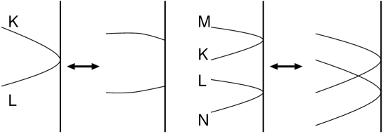
Figure 11: Open string interaction

In the open/closed string field theory, we need to introduce seven types of the string interaction vertices [8]. This is because the the global topology of interaction vertex becomes rather involved and we need the vertex operator for each of them. In the matrix string approach, all of these vertices can be described in terms of one vertex $\Phi_{KL}$ [34]. This is again a great benefit of the current formalism.

In case of the string field theory, the gauge invariance of the string fields requires the gauge group should be $SO(2^{13})$ [8]. Although we have not attempted the consistency of the vertex operator, it should reproduce the similar condition. This is one of the most important issues which should be clarified in the future.

In our discussion in section 5, we emphasized that there are no big difference between the boundary/cross-cap states and the joint states. They are three equally possible boundary states from the viewpoint of the short strings. This aspect is clearer in the action of the interaction vertex (9.1) since it mixes three boundary states. While the boundary states are the representation of the D-brane, the joint states represents a kind of string interaction. In this way, we have seen an interesting mixture of the string dynamics and D-brane. The consistency of the interaction $\Phi_{KL}$ will impose the possible deformation of the joint states from the knowledge of the D-branes and vice versa.

In this paper, we do not make an explicit attempt to incorporate the supersymmetry. A straightforward generalization of the closed string [15] was already made in [34]. These aspects are using the same type of the combinatorics as the bosonic situation does not produce extra non-triviality except for the Chan-Paton factor. One of the difficult point which we would like to indicate is that these vertex operators should intertwine Ramond-Ramond boundary states which describe the D-brane charge and the joint states.

Finally we have to mention that current development of the matrix string theory [29]–[33] where the nontrivial world sheet topology is interpreted as the instanton sectors of 2D Yang-Mills theory. It is quite interesting to investigate if there are similar description of the open string world sheet as the topologically non-trivial sectors in the Yang-Mills theory.

Acknowledgement: The authors would like to thank N. Ishibashi for sending us his thesis [46] which was the essential resource for us to understand the BCFT on orbifolds. One of the authors (Y.M.) is obliged to T. Kawai for the information on DLCQ type partition function and to T. Kawano for explaining the work [8].

Y.M is supported in part by Grant-in-Aid ($\sharp$09640352) and in part by Grant-in-Aid for Scientific Research in a Priority Area: “Supersymmetry and Unified Theory of Elementary Particle” ($\sharp$707) from the Ministry of Education, Science, Sports and Culture.

References

• [1] M.Kaku and K.Kikkawa, “Field Theory of Relativistic Strings. I. Trees”, Phys. Rev. D 10 (1974) 1110-1133; “Field Theory of Relativistic Strings. II. Loops and Pomerons”, Phys. Rev. D 10 (1974) 1823-1843.
• [2] E. Cremmer and J. L. Gervais, “Infinite component field theory of interacting relativistic strings and dual theory”, Nucl. Phys. B90 (1975) 410–460.
• [3] M. R. Green and J. H. Schwarz, “Superstring Interctions”, Nucl. Phys. B218 (1983) 43–88;
“Superfield Theory of Type (II) Superstrings”, Nucl. Phys. B219 (1983) 437–478;
“Superstring Field Theory”, Nucl. Phys. B243 475–536.
• [4] E.Witten, “Non-commutative Geometry and String Field Theory”, Nucl. Phys. B 268 (1986) 79-324;
“Interacting Field Theory of Open Superstring Field Theory”,
Nucl. Phys. B 276 (1986) 291,
• [5] H.Hata, K.Itoh, T.Kugo, H.Kunitomo and K.Ogawa, “Covariant String Field Theory”, Phys. Rev. D 34 (1986) 2360-2429;
“Covariant String Field Theory, II”, Phys. Rev. D 35 (1987) 1318-1355.
• [6] W. Siegel and B.Zwiebach, “Gauge String Fields”, Nucl. Phys. B263 (1986) 105.
• [7] N. Berkovits, “Super Poincare Covariant Quantization of the Superstring”, JHEP 0004 (2000) 018, hep-th/0001035.
• [8] T.Kugo, T.Takahashi, “Unoriented Open-Closed String Field Theory”, Prog. Theor. Phys. 99 (1998) 649-690, hep-th/9711100;
T.Asakawa, T.Kugo and T.Takahashi, “BRS Invariance of Unoriented Open-Closed String Field Theory”, Prog. Theor. Phys. 100 (1998) 831-879;
“One-Loop Tachyon Amplitude in Unoriented Open-Closed String Field Theory”, Prog. Theor. Phys. 102 (1999) 427-466.
• [9] K. Hashimoto, H. Hata, “D-brane and gauge invariance in closed string field theory”, Phys.Rev. D56 (1997) 5179-5193.
• [10] T.Banks, W.Fischler, S.H.Shenker and L.Susskind, “M Theory As A Matrix Model: A Conjecture”, Phys.Rev. D 55 (1997) 5112-5128, hep-th/9610043.
• [11] N. Ishibashi, H. Kawai, Y. Kitazawa, A. Tsuchiya, Nucl. Phys. B496 (1997) 467-491, hep-th/9612115.
• [12] T.Banks, “Matrix Theory”, Nucl. Phys. Proc. Suppl. 67 (1998) 180-224, hep-th/9710231;
D.Bigatti and L.Susskind, “Review of Matrix Theory”, hep-th/9712072.
• [13] L.Motl, “Proposals on Nonperturbative Superstring Interactions”, hep-th/9701025.
• [14] T.Banks and N.Seiberg, “Strings from Matrices”, Nucl. Phys. B 497 (1997) 44-55, hep-th/9702187.
• [15] R.Dijkgraaf, E.Verlinde and H.Verlinde, “Matrix String Theory”, Nucl. Phys. B 500 (1997) 43-61, hep-th/9703030.
• [16] R.Dijkgraaf, E.Verlinde and H.Verlinde, “Notes on Matrix and Micro Strings” Nucl. Phys. Proc. Suppl. 62 (1998) 348-362, hep-th/9709107;
R.Dijkgraaf, “Fields, Strings, Matrices and Symmetric Products”, hep-th/9912104.
• [17] R.Dijkgraaf, G.Moore, E.Verlinde and H.Verlinde, “Elliptic Genera of Symmetric Products and Second Quantized Strings”, Commun. Math. Phys. 185 (1997) 197-209, hep-th/9608096.
• [18] L. Susskind, “Another conjecture about M(atrix) theory”, hep-th/9704080.
• [19] R.Dijkgraaf, E.Verlinde and H.Verlinde, “BPS Spectrum of the Five-Brane and Black Hole Entropy”, Nucl.Phys. B 486 (1997) 77-88, hep-th/9603126;
“5D Black Holes and Matrix Strings”, Nucl. Phys. B 506 (1997) 121-142, hep-th/9704018.
• [20] R.Dijkgraaf, J.Maldacena, G.Moore and E.Verlinde, “A Black Hole Farey Tail”, hep-th/0005003.
• [21] G.E.Arutyunov and S.A.Frolov, “Virasoro Amplitude from the $S^{N}{{\bf R}}^{24}$ Orbifold Sigma Model”, Theor. Math. Phys. B 114 (1998) 43-66, hep-th/9708129;
“Four Graviton Scattering Amplitude from $S^{N}{{\bf R}}^{8}$ Supersymmetric Orbifold Sigma Model”, Nucl.Phys. B 524 (1998) 159-206, hep-th/9712061;
G.E. Arutyunov, S. Frolov and A. Polishchuk, “On Lorentz invariance and supersymmetry of four particle scattering amplitudes in $S^{N}{\bf R}^{8}$ orbifold sigma model”, Phys.Rev. D60 (1999) 066003, hep-th/9812119.
• [22] A. Jevicki, M. Mihailescu and S. Ramgoolam, “Gravity from CFT and $S^{N}(X)$: Symmetries and Interactions” hep-th/9907144.
• [23] T.Banks and L.Motl, “Heterotic Strings from Matrices”, JHEP 9712 (1997) 004, hep-th/9703218.
• [24] D.A.Lowe, “Heterotic Matrix String Theory”, Phys.Lett. B 403 (1997) 243-249, hep-th/9704041.
• [25] S.-J.Rey, “Heterotic M(atrix) Strings and Their Interactions”, Nucl.Phys. B 502 (1997) 170-190, hep-th/9704158.
• [26] P.Bantay, “Characters and modular properties of permutation orbifolds”, Phys.Lett. B 419 (1998) 175-178, hep-th/9708120;
“Permutation orbifolds”, hep-th/9910079;
• [27] T.Kawai, “K3 Surfaces, Igusa Cusp Form and String Theory”, hep-th/9710016;
T. Kawai and K. Yoshioka, “String Partition Function and Infinite Products”, hep-th/0002169.
• [28] H. Nakajima, “Lectures on Hilbert Schemes of Points on Surfaces”, University Lecture Series (Providence, R.I.), No. 18, American Mathematical Society, 1999.
• [29] T. Wynter, “Gauge fields and interactions in matrix string theory” Phys. Lett. B415 (1997) 349, hep-th/9709029;
“High energy scattering amplitudes in matrix string”, hep-th/9905087.
• [30] S. B. Giddings, F. Hacquebord and H. Verlinde, “High energy scattering and D-pair creation in matrix string theory” Nucl. Phys. B537 (1999) 260, hep-th/9804121.
• [31] G. Bonelli, L. Bonora and F. Nesti, “String interactions from matrix string theory” Nucl. Phys. B538 (1999) 100, hep-th/9807232.
• [32] G. Bonelli, L. Bonora and F. Nesti and A. Tomasiello, “Matrix string theory and its moduli space”, Nucl. Phys. B554 (1999) 103, hep-th/9901093.
• [33] P. Brax, “The supermoduli space of matrix string theory” hep-th/9912103.
• [34] C.V.Johnson, “On Second-Quantized Open Superstring Theory”, Nucl.Phys. B 537 (1999) 144-160, hep-th/9806115.
• [35] C.V.Johnson, “Études on D-brane”, hep-th/9812196.
• [36] P. Horava, “Strings on world-sheet orbifolds”, Nucl. Phys. B327 (1989) 461–484.
• [37] K. Ezawa, Y.Matsuo, K.Murakami, “Matrix Model for Dirichlet Open String”, Phys.Lett. B 439 (1998) 29-36, hep-th/9802164.
• [38] C.G.Callan, C.Lovelace, C.R.Nappi and S.A.Yost, “String loops corrections to beta functions,” Nucl. Phys. B288 (1987) 525;
“Adding holes and crosscaps to the superstring,” Nucl. Phys. B293 (1987) 83;
“Loop corrections to superstring equations of motion ,” Nucl. Phys. B308 (1988) 221.
• [39] J.Polchinski and Y.Cai, “Consistency of Open Superstring Theories”, Nucl. Phys. B 296 (1988) 91-128.
• [40] J.L.Cardy “Boundary Conditions, Fusion Rules and the Verlinde Formula”, Nucl. Phys. B 324 (1989) 581-596.
• [41] T.Onogi and N.Ishibashi, “Conformal Field Theories on Surfaces with Boundaries and Crosscaps”, Mod. Phys. Lett. A4 (1989) 161-168.
• [42] N.Ishibashi, “The Boundary and Crosscap States in Conformal Field Theories”, Mod. Phys. Lett. A 4 (1989) 251-264.
• [43] P.Di Vecchia and A.Liccardo, “D Branes in String Theory, I”, hep-th/9912161;
“D Branes in String Theory, II”, hep-th/9912275.
• [44] J.A.Harvey and J.A.Minahan, “Open Strings on Orbifolds”, Phys. Lett. B 188 (1987) 44-50.
• [45] N.Ishibashi and T.Onogi, “Open String Model Building”, Nucl. Phys. B 318 (1989) 239-280.
• [46] N. Ishibashi, “Open String Model Building”, Ph. D. thesis, University of Tokyo, 1990.
• [47] G.Pradisi and A.Sagnotti, “Open String Orbifolds”, Phys. Lett. B216 (1989) 59-67.
• [48] A. Recknagel and V. Schomerus, “D-branes in Gepner models” Nucl. Phys. B531 (1998) 185-225.
• [49] D.-E. Diaconescu and J. Gomis, “Fractional Branes and Boundary states in Orbifold Theories” hep-th/9906242.
• [50] I. Brunner, M. R. Douglas, A. Lawrence and C. Römelsberger, “D-branes on the Quintic”, hep-th/9906200.
• [51] R. E. Behrend, P. A. Pearce, V. B. Petkova, J.-B. Zuber, “Boundary Conditions in Rational Conformal Field Theory”, Nucl.Phys.B570 (2000) 525–589, hep-th/9908036.
• [52] P. Bantay, “Symmetric products, permutation orbifolds and discrete torsion”, hep-th/0004025;
Z.Kadar, “The torus and the Klein Bottle amplitude of permutation orbifolds”, hep-th/0004122.
• [53] G. Grignani and G. W. Semenoff, “Thermodynamic partition function of matrix superstring”, Nucl. Phys. B561 (1999) 243, hep-th/9903246.
• [54] G. Grignani, P. Orland, L. D. Paniak, and G. W. Semenoff, “Matrix Theory Interpretation of DLCQ String Worldsheets” hep-th/0004194.
• [55] J.-P.Serre, “A Course in Arithmetics”, Graduate Texts in Mathematics 7, Springer-Verlag, 1973.
• [56] T.M.Apostol, “Modular Functions and Dirichlet Series in Number Theory”, Graduate Texts in Mathematics 41, Springer-Verlag, 1976.
• [57] A. Sen, “Universality of tachyon potential”, JHEP 9912 (1999), 027. hep-th/9911116.
• [58] A. Sen and B. Zwiebach, “Tachyon condensation in string field theory” JHEP 0003 (2000) 002, hep-th/9912249.
• [59] N. Berkovits, A. Sen and B. Zwiebach, “Tachyon condensation in superstring field theory”, hep-th/0002211