Holography and Riemann Surfaces

Abstract

We study holography for asymptotically AdS spaces with an arbitrary genus compact Riemann surface as the conformal boundary. Such spaces can be constructed from the Euclidean ${\rm AdS}_{3}$ by discrete identifications; the discrete groups one uses are the so-called classical Schottky groups. As we show, the spaces so constructed have an appealing interpretation of “analytic continuations” of the known Lorentzian signature black hole solutions; it is one of the motivations for our generalization of the holography to this case. We use the semi-classical approximation to the gravity path integral, and calculate the gravitational action for each space, which is given by the (appropriately regularized) volume of the space. As we show, the regularized volume reproduces exactly the action of Liouville theory, as defined on arbitrary Riemann surfaces by Takhtajan and Zograf. Using the results as to the properties of this action, we discuss thermodynamics of the spaces and analyze the boundary CFT partition function. Some aspects of our construction, such as the thermodynamical interpretation of the Teichmuller (Schottky) spaces, may be of interest for mathematicians working on Teichmuller theory.

I Introduction

In this paper we apply the idea of bulk/boundary correspondence to a particular large class of asymptotically AdS spaces. More precisely, we study holography in 2+1 dimensions, and the spaces we consider have non-trivial boundary topology. As we show, the holographic prescription can be meaningfully extended to the case of manifolds with any Riemann surface as the conformal boundary.

We wish to emphasize from the outset that the paper is “classical” in its spirit - no stringy aspects of the idea of holography is used. Our analysis of the boundary CFT is based on the semi-classical approximation to the gravity path integral. Thus, our results will pertain, in the regime of validity of this approximation, to any quantum gravity theory in 2+1 dimensions, in case any such consistent theory other than string theory is ever constructed in the future.

The idea to study holographically dual CFT’s for arbitrary topology of the boundary can be suggested by purely conformal field theory considerations. Indeed, two dimensional CFT’s certainly do make sense on any genus Riemann surface. In fact, any CFT can be viewed as exactly the structure that endows the moduli space of Riemann surfaces with analytic geometry [18]. Moreover, knowing the CFT partition function for arbitrary genus allows one to reconstruct all correlation functions. This is done by varying the moduli so as to “pinch” handles of the Riemann surface; the correlation functions can then be read off from the leading order terms of the expansion in the moduli, see [18]. Thus, from the CFT point of view, it is quite natural to allow the genus and moduli to be variable.

Another CFT reason to consider different topologies is the fact that certain vertex operators can “change” the topology of the surface where the theory lives. These are the multi-valued operators, such as fermionic vertex operators or certain operators in orbifold constructions. When one calculates correlation functions of such operators, it is very convenient, and sometimes necessary, to introduce the universal cover of the worldsheet. One then gets Riemann surfaces of various genera; the classical fact that a Riemann surface of genus $g$ covers the sphere $g+1$ times is a good illustration. See [20] for various examples.

Last, but not least of our motivations, is that, as is demonstrated in the next section, asymptotically AdS spaces with non-trivial boundary topology are, in certain precise sense, the “analytic continuations” to the Euclidean signature of the well-known black hole solutions. A particularly interesting set of black hole solutions consists of black holes with a single asymptotic region and an arbitrary genus wormhole contained inside the horizon. As we show in the next section, the boundary of the Euclidean counterparts of these spacetimes is a Riemann surface, whose genus is twice the genus of the wormhole. Thus, extending the ideas of holography to Euclidean spaces of non-trivial boundary topology is a step towards the holographic description of these black hole spacetimes. Potentially, this gives a way towards understanding whether the holography can “see” the part of spacetime hidden behind the horizon.

Let us now, for the sake of readers who are not familiar with it, review the very basics of the idea of holography, in the amount that is needed for the purposes of this paper. In broad terms holography is a description of a theory in $n+1$ dimensions by another theory in $n$ dimensions. Numerous examples of such a description were recently found in string theory, see [1] for a review. The holographic prescription of [19, 42] states that the generating functional of the boundary field theory is given by the bulk path integral, with sources being just the (appropriately rescaled) boundary values of the bulk fields. If one is only interested in correlation functions of the boundary stress-energy tensor, one should put sources for all other boundary operators to zero. Thus, the generating functional of correlation functions of the stress-energy tensor (or CFT partition function) is given by the bulk gravity path integral. The source is just the (appropriately rescaled) boundary value of the metric, and the path integral sums over all bulk metrics approaching this fixed boundary value. The semi-classical approximation to this path integral is given by the sum over all classical solutions of Einstein equations that approach a fixed metric at the boundary.

Thus, to find the semi-classical approximation to the boundary CFT partition function, we have to identify all classical solutions that approach a prescribed metric at the boundary. This is done in Section II, where we describe Euclidean spaces of constant negative curvature whose conformal boundary is an arbitrary Riemann surface. These are classical results, dating back to the work of Poincare on Kleinian groups. In this section we also discuss the “spacetime” interpretation of the Euclidean spaces constructed. We show that in certain precise sense they are “analytic continuations” to Euclidean signature of physically interesting black hole solutions. The CFT partition function is then studied in Section III. Here we describe the regularization procedure that is needed to render the on-shell gravity action finite, discuss the thermodynamics of our Euclidean spaces, and analyze the resulting CFT partition function. We conclude with a discussion.

An important role in this paper is played by the results of Takhtajan and Zograf [38] on the Liouville theory on Riemann surfaces. We “derive” the action proposed in [38] using the bulk/boundary prescription. Thus, this paper gives a new, (2+1)-dimensional interpretation to the results that were obtained based on purely two-dimensional considerations. Moreover, our observation that the Euclidean spaces considered can be interpreted as the “analytic continuations” of the black hole spacetimes allowed us to give the results of [38] a thermodynamical interpretation.

Most of the mathematics background of this paper, including the definition of the Liouville action for any Riemann surface, and results on the dependence of this action on the moduli, is from work [38]. To make the paper self-consistent, some of this material is repeated here. Thus, the relevant facts on Schottky groups are reviewed in II A, and some facts about Liouville theory on Riemann surfaces are reviewed in III C. The Appendix reviews aspects of the theory of Teichmuller spaces, which play an important role in our story.

There exists a rather large literature on bulk/boundary correspondence in 2+1 dimensions and we would like to mention few papers that are somewhat related to the present work. Thus, the correspondence for the boundary topology different from that of a sphere was discussed in [7, 44]. The genus one case was discussed in [6, 12]. A relation between geometry of hyperbolic manifolds and the boundary CFT was discussed in [27]. Finally, the observation that the Liouville action appears as the effective action on the boundary was made in [37, 36, 5].

II Classical solutions

This section consists of two parts. Subsection II A describes Euclidean Einstein manifolds of constant negative curvature that have a Riemann surface as the boundary. The spaces of interest are well-known since the work of Poincare on Kleinian groups. These are the spaces obtained by discrete identifications of AdS₃ using Schottky groups. All facts discussed in this subsection are well-known. Subsection II B discusses the Lorentzian signature interpretation of the spaces. This interpretation is, to the best of our knowledge, new.

A Euclidean case

In three dimensions all constant negative curvature Einstein manifolds are locally indistinguishable from the AdS space. Thus, they can be obtained by an appropriate identification of points in AdS.

In what follows, we shall mostly use the upper half-space model of AdS. We denote the upper half-space by ${\bf H}$, which stands for the ‘hyperbolic space’. The hyperbolic metric on ${\bf H}$ is:

$$ds^{2}={l^{2}\over z^{2}}(dx^{2}+dy^{2}+dz^{2}),$$ (1)

where $l$ is the curvature radius. The group of isometries of ${\bf H}$ is ${\rm SL}(2,{\mathbb{C}})$. The boundary ${\bf S}$ of ${\bf H}$ is at $z=0$, plus the point at infinity. Thus the boundary is just the Riemann sphere, and ${\rm SL}(2,{\mathbb{C}})$ acts on ${\bf S}$ by conformal transformations. This action of ${\rm SL}(2,{\mathbb{C}})$ on ${\bf S}$ can be described most elegantly by introducing the complex coordinate $w=x+iy$. Then the action of ${\rm SL}(2,{\mathbb{C}})$ on ${\bf S}$ is given by fractional linear transformations (or Mobius transformations):

$$w\to{aw+b\over cw+d},\qquad a,b,c,d\in{\mathbb{C}},\qquad ad-bc=1.$$ (2)

The action of ${\rm SL}(2,{\mathbb{C}})$ on ${\bf H}$ itself can also be represented in terms of fractional linear transformations; this is done by introducing quaternionic coordinates in the upper half-space, see, e.g., [15] for details of this construction.

In what follows we will need some basic facts about the ${\rm SL}(2,{\mathbb{C}})$ action in ${\bf H}$. The geodesics are semi-circles that intersect the boundary ${\bf S}$ orthogonally (lines orthogonal to ${\bf S}$ included). Transformations from ${\rm SL}(2,{\mathbb{C}})$ map geodesics to geodesics. The geodesic surfaces of ${\bf H}$ are hemispheres intersecting the boundary orthogonally (the planes orthogonal to ${\bf S}$ included). Geodesic surfaces are mapped to geodesic surfaces. An important fact about the action of ${\rm SL}(2,{\mathbb{C}})$ is that each such transformation can be represented by an even number of inversions in hemispheres in ${\bf H}$.

One can obtain constant negative curvature spaces other than ${\bf H}$ identifying its points by the action of some discrete subgroup of ${\rm SL}(2,{\mathbb{C}})$. To describe the action of such a group it is very convenient to concentrate on its action on the boundary. Let $\Delta$ be the (closure of the) set of fixed points of this action. Thus, by definition $\Delta$ is a closed set. If it does not coincide with the whole of ${\bf S}$, the group is called a Kleinian group. We denote Kleinian groups by $\Sigma$. Then $\Omega={\bf S}\backslash\Delta$ is an open set on which $\Sigma$ acts discontinuously. It is called the region of discontinuity of $\Sigma$. The quotient $X=\Omega/\Sigma$ is a smooth manifold. For what follows we will also need the notion of a fundamental region for $\Sigma$. It is a set $D\subset\Omega$, such that no two distinct interior points of $D$ are $\Sigma$-equivalent, and every point of $\Omega$ is $\Sigma$-equivalent to some point of $D$. We shall see examples of fundamental regions below. For more information on Kleinian groups see, e.g., [33]. Extending the action of $\Sigma$ to the whole ${\bf H}$, and identifying points that are $\Sigma$-related, one gets a space of constant negative curvature whose boundary is $X$.

Varying $\Sigma$ one gets a plethora of spaces, some of them of complicated topology. In this paper we shall consider only rather special Kleinian groups, known as classical Schottky groups. These are the simplest, and most studied examples of Kleinian groups. They were first discovered by Schottky and Klein, and then studied in detail by Poincare more than a hundred years ago. As we shall see in a moment, it is these groups that lead to compact Riemann surfaces as boundaries. Thus, they are general enough for the purpose of this paper, which is to study the holography on manifolds bounded by Riemann surfaces. Unlike the spaces one gets for more complicated Kleinian groups, the spaces associated with the classical Schottky groups also admit a direct Lorentzian interpretation, as we shall see in the next subsection. We only consider classical Schottky groups in this paper.

A Schottky group $\Sigma_{g}$ of genus $g$ is (freely) generated by a finite number $g$ of loxodromic generators $L_{1},\ldots,L_{g}$ (a group element is called loxodromic if it is conjugate, in the group of all Mobius transformations, to a transformation of the form $w\to w/\lambda,|\lambda|>1$). The number $g$ of generators of a Schottky group $\Sigma$ is exactly the genus of the resulting quotient space $X$. We also need the notion of a marked Schottky group. A Schottky group is called marked if the set of its generators is ordered.

A marked Schottky group is most conveniently described by its fundamental region. Let $C_{1},\ldots,C_{g},C_{1}^{\prime},\ldots,C_{g}^{\prime}$ be $2g$ non-intersecting circles in ${\bf S}$ such that all circles lie to the exterior of each other. Let $L_{i}$ be the loxodromic element mapping $C_{i}$ to $C_{i}^{\prime}$ so that the region exterior to $C_{i}$ is mapped to the interior of $C_{i}^{\prime}$. Then the group $\Sigma_{g}$ freely generated by the elements $L_{1},\ldots,L_{g}$ is a Schottky group, its fundamental region is the part of ${\bf S}$ exterior to all circles, and the quotient space is a compact Riemann surface of genus $g$. To convince oneself that the quotient space obtained this way is indeed a genus $g$ Riemann surfaces it is best to picture the boundary as $S^{2}$. Cutting out of this sphere $2g$ discs one gets a manifold with a boundary, the boundary being just the collection of circles $C_{1},\ldots,C_{g},C_{1}^{\prime},\ldots,C_{g}^{\prime}$. One then identifies the circles to obtain a manifold without boundary, which is just a $g$-handled sphere.

Using the freedom of conjugating all generators by some Mobius transformation, one can choose the fundamental region in the canonical way. Each generator $L_{i}$ is completely characterized by its two fixed points (because all $L_{i}$ are strictly loxodromic these points are distinct), and the value of its multiplier $\lambda_{i}$. The geometrical meaning of the multiplier is to specify by “how much” the corresponding transformation moves things along the geodesics connecting the fixed points. Let us denote the attractive fixed point of $L_{i}$ by $a_{i}$ and its repulsive fixed point by $b_{i}$. Then, by conjugation in the group of all Mobius transformations, we can put $a_{1}=0,b_{1}=\infty,a_{2}=1$. A Schottky group for which these conditions hold is called normalized.

Let $\Sigma_{g}$ be a marked Schottky group of genus $g$. The map

$$\Sigma_{g}\to(a_{3},\ldots,a_{g},b_{2},\ldots,b_{g},\lambda_{1},\ldots,\lambda_{g})\in{\mathbb{C}}^{3g-3}$$ (3)

establishes a one-to-one correspondence between the set of marked Schottky groups and some subset of ${\mathbb{C}}^{3g-3}$. This subset can be shown to be a connected region, and is called the Schottky space of genus $g$. We will denote it by ${\mathfrak{S}}_{g}$. Because of its dimension (real 6g-6) one is tempted to think that the Schottky space ${\mathfrak{S}}_{g}$ is related in some way to the moduli space of Riemann surfaces of genus $g$. This is indeed the case, the moduli space $R_{g}$ turns out to be a certain quotient of ${\mathfrak{S}}_{g}$, as we shall explain below.

The classical retrosection theorem due to Koebe states that every compact Riemann surface $X$ can be represented as the quotient $\Omega/\Sigma$, where $\Sigma$ is a Schottky group with region of discontinuity $\Omega$. Moreover, one can always choose a Schottky group and the fundamental region in such a way that a given set of $g$ generators of $\pi_{1}(X)$ is the image of circles $C_{i}$ under the quotient map. More precisely, given a basis of generators

$$\alpha_{1},\ldots,\alpha_{g},\beta_{1},\ldots,\beta_{g}:\prod_{i=1}^{g}[\alpha_{i},\beta_{i}]=1,\qquad[\alpha,\beta]=\alpha^{-1}\beta^{-1}\alpha\beta$$ (4)

of $\pi_{1}(X)$, one can choose a marked Schottky group $\Sigma_{g}$ and $g$ generators $L_{1},\ldots,L_{g}$ of $\Sigma_{g}$ so that there is a standard fundamental region $D$ bounded by $C_{1},\ldots,C_{g},C_{1}^{\prime},\ldots,C_{g}^{\prime}$ with $L_{i}(C_{i})=C_{i}^{\prime}$ such that: (i) $\alpha_{i}$ is the image of $C_{i}$ under the quotient map $\Omega\to\Omega/\Sigma_{g}$; (ii) the group of the covering $\Omega\to\Omega/\Sigma_{g}$ coincides with the smallest normal subgroup ${\cal N}$ of $\pi_{1}(X)$ containing elements $\alpha_{1},\ldots,\alpha_{g}$; (iii) group $\Sigma_{g}$ is isomorphic to the factor group $\pi_{1}(X)/{\cal N}$. A proof of this theorem can be found, e.g., in [17]. For more information on Schottky groups see [38] and references therein.

Thus, all compact Riemann surfaces arise as quotients of ${\bf S}$ by classical Schottky groups. This fact allows one to use the space of all Schottky groups –the Schottky space– to coordinatize the space of Riemann surfaces. The problem is that several points in the Schottky space may correspond to the same Riemann surface. This turns out to be indeed the case, see [22]. Thus, to get from ${\mathfrak{S}}_{g}$ to the space of Riemann surfaces $R_{g}$ one performs certain identifications. This is discussed in more details in the Appendix.

The procedure of associating a compact Riemann surface with a Schottky group such that the Riemann surface is represented as the quotient space is called uniformization by Schottky groups. There is another well-known uniformization procedure –the so-called uniformization by Fuchsian groups– that we will encounter below.

To summarize, we see that one can get constant negative curvature manifolds whose boundary is a Riemann surface by doing identifications of points in AdS₃ by the action of a Schottky group. Moreover, the retrosection theorem guarantees that all Riemann surfaces arise as boundaries of the spaces so constructed.

Let us now illustrate this construction on the examples of $g=1,2$.

Example A: g=1

The genus one case is different from all higher genus cases, for it is uniformized by the zero curvature space, while all higher genus surfaces are uniformized by the space of negative curvature. Also, the (real) dimension of its moduli space (which is two) does not follow the $6g-6$ formula of the higher genus cases. Still, it gives a good illustration of the general construction. It is also of direct physical relevance, for the corresponding space describes, e.g., the AdS space at finite temperature and BTZ black hole.

The genus one Schottky groups are generated by a single loxodromic element $L$. Thus, elements of such a group are simply powers of the generator (and its inverse). The set $\Delta$ of fixed points consists in this case of only two points: the attractive and repulsive fixed points of the element $L$. This is an example of the so-called elementary Schottky groups.

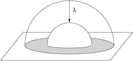
FIG. 1.: Genus one case.

The fundamental domain for a normalized Schottky group of genus one is an annulus centered at $w=0$, see Fig. 1. The transformation $L$ maps the upper hemisphere to the lower one. Thus, the Euclidean space that one gets after the identifications have been made is just the region between the hemispheres, with the hemispheres being identified. As is clear from the figure, this space is a solid torus. Having put the fixed points of $L$ to $w=0,\infty$, the only parameter left is the multiplier $\lambda$ . The geometrical meaning of $\lambda$ is that its absolute value is the distance between the hemispheres, while its argument is the angle by which one hemisphere is rotated with respect to the other in the identification. One can already recognize the Euclidean BTZ black hole in this space, with its angular coordinate running along the geodesics connecting the hemispheres. We discuss this relation in more details in the next subsection, where the Lorentzian interpretation of our spaces is considered.

The Schottky space in this case is the space of $\lambda:|\lambda|>1$. Because of the hole $|\lambda|<1$ in it, it is not simply connected. It is universally covered by the Teichmuller space. The Teichmuller space can be modeled by the upper half-plane. This is done by introducing the modular parameter:

$$\tau={{\rm Arg}\lambda\over 2\pi}+i{\ln{|\lambda|}\over 2\pi}.$$ (5)

The Schottky space is then just the strip $|{\rm Re}\tau|<1/2$. Because of the identifications of the sides of the strip, the Schottky space is not simply connected, and its universal cover –the Teichmuller space– is the whole upper half-plane. The corresponding Riemann space, i.e., the space of different conformal structures of the $g=1$ case, is the quotient of this space with respect to the action of the modular group, which in this case is ${\rm PSL}(2,{\mathbb{Z}})$. This is the general situation: the Schottky space is not simply connected, and its universal cover is just the Teichmuller space. The Riemann space is a quotient of the Teichmuller (and Schottky) spaces, see [22].

Example B: g=2

This is a much more complicated case. It gives a good intuition about what happens for higher genera. A $g=2$ Schottky group is generated by two elements $L_{1},L_{2}$. Thus, its elements are all “words” constructed from “letters” $L_{1},L_{2}$ and their inverses. The (completion of the) set of fixed points in this case is a Kantor set, of measure zero in ${\bf S}$.

A normalized Schottky group is obtained by conjugating the generator $L_{1}$ so that its fixed points lie at $w=0,\infty$, and conjugating $L_{2}$ to bring its attractive fixed point at $w=1$. The fundamental region then looks like that in Fig. 2 The transformation $L_{1}$ identifies the upper and lower hemispheres, while $L_{2}$ maps left to the right one. As is clear from the figure, the fundamental domain becomes a genus two surface after identifications. Thus, the Euclidean space one gets is a solid two-handled sphere. In the next subsection we shall see that such solid two handled spheres are Euclidean versions of, for example, the known [2] single asymptotic region wormhole solution, and of three asymptotic region black hole.

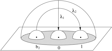
FIG. 2.: Genus two case.

Let us now calculate the number of parameters describing the $g=2$ case. They are: the multipliers $\lambda_{1},\lambda_{2}$ of both generating transformations, plus the complex coordinate $b_{2}$ of the repulsive fixed point of the second generator. Thus, we have in total 6 real parameters. The Schottky space, however, cannot be described so explicitly as in the case of $g=1$. The general result only tells us that this space is a connected region in ${\mathbb{C}}^{3}$. Also, particular boundary points can be obtained by an explicit hard labor calculation.

As in the genus one case, the Schottky space is not simply connected; its universal cover is the Teichmuller space of genus two. The corresponding Riemann space can be obtained as a quotient of each of these spaces.

B Lorentzian interpretation

We now proceed to the Lorentzian signature interpretation of the spaces described above. Although the Lorentzian spacetimes of this subsection were known before, the fact that these spacetimes have natural “analytic continuations”, where they become solid $g$-handled spheres, to the best of our knowledge, was not realized.

We first review some known facts about the black hole solutions in 2+1 dimensions, and then describe a procedure that, given a black hole spacetime, constructs the corresponding Euclidean signature space.

The spacetimes we are going to describe are constant negative curvature spaces, and thus are obtained from Lorentzian AdS₃ by discrete identifications. The corresponding constructions are described in details in [2, 3]; we shall only sketch them here.

Let us first consider the non-rotating case [2]. The relation between the spaces described above and the Lorentzian signature black holes is most transparent in this case. The case of rotating black holes is somewhat more complicated; we discuss it at the end of this subsection.

The characteristic feature of non-rotating spacetimes of [2] is that there is a surface of time symmetry. Let us call it the $t=0$ hypersurface. Because it is time symmetric, its extrinsic curvature vanishes. Thus, it is a two-dimensional Euclidean signature space of constant negative curvature. Such spaces are all obtainable by identifications of points of AdS₂, and are easy to classify by specifying the discrete group of identifications that was used. Having described the geometry of $t=0$ plane, one then “evolves” this geometry forwards and backwards in time to obtain the whole spacetime.

FIG. 3.: BTZ black hole: the initial slice geometry.

Let us now describe the possible $t=0$ slice geometries. There are two basic possibilities: the geometry can be either compact or non-compact.

The compact case is well-known from the theory of uniformization of Riemann surfaces. The discrete groups one uses are the so-called Fuchsian groups. The fundamental region in this case is a $4G$-sided polyhedron in AdS₂. A Fuchsian group is a discrete subgroup of the group of isometries, i.e., subgroup of ${\rm SL}(2,{\mathbb{R}})$. It is generated by $2G$ elements, with one relation between them. The geometries that arise are compact genus $G$ Riemann surfaces.

The spacetimes one gets by evolving such compact $t=0$ slice geometries are expanding and then collapsing compact universes. In other words, they appear at some moment in past from the past singularity, and disappear in the future singularity in finite time. Such spacetimes may be interesting as simple cosmological models. They were studied in this context in, e.g., [31].

The black holes of [2] realize the other possibility: non-compact $t=0$ surface. They are still obtainable from AdS₂ by discrete identifications by Fuchsian groups (by which we mean discrete subgroups of ${\rm SL}(2,{\mathbb{R}})$); these are, however, not the “classical” Fuchsian groups, for one gets non-compact surfaces. Thus, in this case, the initial time geometry will have asymptotic regions. Evolving these asymptotic regions, one gets the asymptotic regions of the corresponding spacetime. These will generally occupy only a finite region on the boundary of the Lorentzian AdS₃. Then the boundaries of the past of these asymptotic regions will have the interpretation of event horizons: one gets black holes.

It is instructive to see how the usual BTZ black hole can be obtained this way. The $t=0$ slice of the BTZ black hole is shown in Fig. 3(a); following [2] we use the unit disc model for AdS₂. The corresponding discrete group (subgroup of ${\rm SU}(1,1)\simeq{\rm SL}(2,{\mathbb{R}})$) is generated by a single element. The fundamental region is the “strip” between the two geodesics; one of them is mapped into the other by the generator. The quotient space has the topology of the $S^{1}\times{\mathbb{R}}$ wormhole with two asymptotic regions, each having the topology of $S^{1}$, see Fig. 3(b). The BTZ angular coordinate runs from one geodesics to the other. The distance between the two geodesics measured along their common normal is precisely the horizon circumference.

FIG. 4.: BTZ black hole: the spacetime picture. Two asymptotic regions are shown: they are parts of the boundary cylinder lying between the timelike geodesics. The future event horizon, which is the boundary of the past of the asymptotic infinity, is shown. Note that it intersects the initial slice along the minimal line connecting the two geodesics bounding the fundamental region.

One can obtain the spacetime geometry of this black hole by “evolving” the $t=0$ slice geometry. In this evolution, geodesics of the initial slice evolve into geodesic surfaces in the spacetime, which are then to be identified. The region between them, after identifications, is the BTZ black hole spacetime, see Fig. 4. Because timelike geodesics in AdS are “attracted” to each other, the two geodesic surfaces will finally cross. This is where the spacetime “ends”. Note, however, that the time it takes for them to meet each other is finite only in the global AdS time coordinate. In BTZ time coordinate the corresponding “singularities” are at past and future infinity. The asymptotic infinity of the BTZ black hole consists of two regions on the AdS boundary cylinder. These are the regions between the timelike geodesics on the boundary; the geodesics are identified. One can now construct the past of the asymptotic region to convince oneself that there is a region in this spacetime that is causally disconnected from the infinity, see Fig. 4. This region is the black (white) hole, and its boundary is the event horizon.

Let us now, following [2], consider more complicated initial slice geometries. Let the fundamental region to be the part of the unit disc between four geodesics, as in Fig. 5(a). Let us identify these geodesics cross-wise. It is straightforward to show that the resulting geometry has only one asymptotic region, consisting of all four parts of the infinity of the fundamental region. With little more effort one can convince oneself that the resulting geometry is one asymptotic region “glued” to a torus, see Fig. 5(b). Considering the spacetime that one gets by evolving this geometry, one finds that this is a single asymptotic region black hole, but the topology inside the event horizon is now that of a torus. See [2] for more details on this spacetime.

Another interesting and simple spacetime is that containing three asymptotic region black hole [2]. The fundamental region on the $t=0$ plane is again the region bounded by four geodesics. They are, however, now identified side-wise, see Fig. 6(a). One can clearly see that the initial slice geometry has three asymptotic regions, as in Fig. 6(b). Evolving this, one gets a spacetime with three asymptotic regions and corresponding event horizons. See [2] for more details.

This procedure allows one to construct a large variety of spacetimes, see [2]. In particular, one can have a single asymptotic region black hole with an arbitrary Riemann surface inside the horizon.

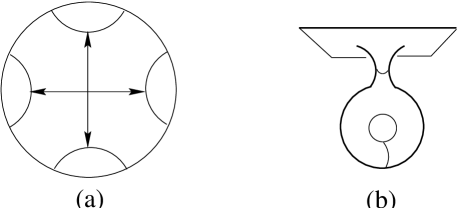
FIG. 5.: Initial slice geometry of the single asymptotic region black hole with a toroidal wormhole inside the horizon

FIG. 6.: Initial slice geometry of the three asymptotic region black hole

The construction of black hole spacetimes we just described is well-known. It was not realized, however, that there exists a natural way to “analytically continue” these spacetimes into the Euclidean signature. As we shall see in a moment, the Euclidean spaces one obtains are just the spaces constructed in the previous subsection.

All the spacetimes described were obtained by discrete identifications of points of the Lorentzian signature AdS₃. Let us try to construct their Euclidean analogs; the basic idea is to identify points in Euclidean AdS₃ using the “same” transformations as the ones that were used in the Lorentzian case. We must be careful, however, about what the “same” means, for the groups of isometries in these two cases are different. In the case of non-rotating black holes, however, there is a natural choice. Indeed, in spacetimes we described there is a surface whose geometry locally is that of Euclidean AdS₂. Let us require that in the Euclidean spaces we are going to construct there is also a surface of “time symmetry”, whose geometry coincides with the geometry of $t=0$ slice of the Lorentzian case. One can now “evolve” this geometry in the Euclidean “time” to obtain the whole Euclidean space. It is easy to see that this procedure determines the Euclidean geometry completely, once the geometry of the $t=0$ slice of the Lorentzian case is specified.

Let us see how this works for the simplest case of BTZ black hole. Let us use the unit ball model for the Euclidean AdS₃. Thus, we require that the geometry of one of the slices of this ball going through the origin is the same as the geometry of the $t=0$ slice of BTZ black hole, see Fig. 3. We then simply have to continue the geodesics that are identified on the $t=0$ slice to geodesics surfaces in AdS₃; one gets two hemispheres, as in Fig. 7(a). The Euclidean BTZ black hole is then the region between these hemispheres; the hemispheres themselves are identified. To represent this space in the form already familiar to us, let us map the unit ball into the upper half-space. Let us also “normalize things” by putting the fixed points to $z=0,\infty$. What we get is two hemispheres centered at $z=0$. The Euclidean BTZ is the region between the hemispheres. The $t=0$ slice of our original Lorentzian signature black hole is now simply the $y=0$ slice. The horizon is represented in the Euclidean picture by the part of the $x=y=0$ line that is contained between the hemispheres. The distance between the hemispheres along that line is the horizon circumference. The geometry we got is, of course, just the usual Euclidean BTZ hole geometry that can be obtained from the Lorentzian signature BTZ metric by the analytic continuation of the time coordinate, see [11]. But what we obtained is also just one of the cases considered in the previous subsection. Indeed, it is just the genus one case for the special case when the multiplier $\lambda$ is purely real. The “reality” of $\lambda$ is, of course, the consequence of the fact that we are dealing with the non-rotating BTZ black hole. As we shall see below, allowing $\lambda$ to be complex indeed corresponds to the inclusion of rotation. Thus, using our “analytic continuation” procedure we arrived at the known Euclidean BTZ geometry; we also see that it is just one of the cases considered in the previous subsection, namely, the Euclidean BTZ black hole is a solid torus.

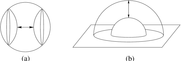
FIG. 7.: Euclidean BTZ black hole

Let us consider another example. We now want to construct the Euclidean version of the single asymptotic region black hole with a torus inside the horizon. The procedure is the same: we require a slice of the unit ball to have the same geometry as the $t=0$ slice of this black hole. This gives us four hemispheres inside the unit ball; the Euclidean space is the region between them and they are to be identified cross-wise, see Fig. 8(a). To help the situation look more familiar, let us again map it into the upper half-space; we put three of the four fixed points to $z=0,\infty,1$, see Fig. 8(b). What we get is one of our genus two case spaces described in the previous subsection. All three parameters $\lambda_{1},\lambda_{2},b_{2}$ are now real; this corresponds to the absence of rotation.

One can do a similar analysis for the three asymptotic region black hole (one also gets a solid two-handled sphere), and for any other of the non-rotating black holes of [2]. In all cases the pattern is the same: one requires the $t=0$ slice geometry to be the same also in the Euclidean case, and this determined the Euclidean geometry completely. The Euclidean spaces one gets are solid $g$-handled spheres of the previous subsection, with all parameters of the Schottky space being real, which corresponds to no rotation.

There is a very simple formula that allows one to calculate the genus of the Euclidean boundary by knowing the number of asymptotic regions and the topology inside the horizon. Let us denote the number of asymptotic regions by $K$, and the genus of the wormhole sitting inside the horizon by $G$. Then the genus $g$ of the Euclidean boundary is given by:

$$g=2G+K-1.$$ (6)

One can easily convince oneself that this formula holds by checking it on few examples. To see this formula in use, let us determine the spaces that have $g=2$. One can easily see that they are: (i) $G=1,K=1$ - single asymptotic region, torus inside the horizon, and (ii) $G=0,K=3$ - three asymptotic regions.

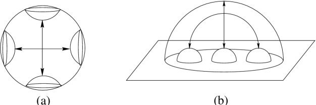
FIG. 8.: Euclidean single asymptotic region black hole with a torus inside

Before we turn to the rotating case, an important remark is in order. As is discussed in details in [2], the geometry of each of the asymptotic regions of the black hole spacetimes described is always the same as that of the asymptotic region of the BTZ black hole of certain mass. What is different in these black holes is only the geometry inside the horizon. This faces us with a puzzle: on one hand, our experience with analytic continuations tells us that the analytic continuation procedure is only sensitive as to what happens outside of the horizon. Thus, one would expect that, since the geometry outside is in all cases the same, the result of the analytic continuation should also be the same. On the other hand, the procedure just described clearly gives different Euclidean spaces, for example for the BTZ black hole and for the single asymptotic region BH with a torus inside. Thus, the “analytic continuation” procedure that we described is different from the usual procedure.

We would now like to convince a skeptical reader that this alternative “analytic continuation” procedure is more natural in our context than the usual one. An important observation here is that the spacetimes we are working with do not have a global Killing vector field generating time translation (actually, no global KVF’s at all). There only is a timelike KVF outside of the horizons, in the asymptotic regions. Inside the horizons, the spacetimes are non-stationary; as discussed in [2], the wormhole sitting inside the horizons evolves, and, in particular, changes its size. The absence of a global KVF is a generic feature of all these spacetimes (except for the BTZ case). Thus, the usual procedure of analytically continuing in the coordinate defined by the time translations KVF seems unnatural in our case, for there is no such global KVF. The procedure described above, however, does not need any such global KVF. Moreover, as we saw above, it gives the same result as the usual analytic continuation procedure in the case of the BTZ black hole, which does have a global time KVF. Thus, in our opinion, the procedure described is an alternative to the usual analytic continuation procedure, which is more natural in the situations where no global KVF corresponding to time translations is present. Of course, as it stands, this alternative procedure is only available in the case of 2+1 gravity; because of the absence of local degrees of freedom here the spacetimes are constructed by discrete identifications, and this is what makes our procedure possible.

Having this said, and hoping that this convinces the reader that the procedure described does make sense, let us now discuss the rotating case. As usual in general relativity, the inclusion of rotation is much harder than one could naively expect it to be. So far, the rotating “wormholes” are much less studied than non-rotating ones. There are essentially only few references on the subject, see [3, 24, 9]. The trick with the time symmetry surface, that greatly simplified the classification of the non-rotating spacetimes, is not available, because there is now no such surface. To construct such spacetimes one takes a different route [3] of studying the action of the discrete group of identifications on the AdS₃ boundary cylinder. This way one can analyze the causal structure of the resulting spacetimes, and it is possible to explicitly compute the mass and angular momentum parameters of the asymptotic regions, see [3] for details. We are not going to use this construction here. Instead, we shall list some facts that, we hope, will convince the reader that the general case Euclidean spaces considered in the previous subsection indeed correspond to rotating black holes.

We have already encountered such facts before. Indeed, we saw that the Euclidean spaces corresponding to non-rotating black holes are just special points in the Schottky space, in the sense that all parameters are real. When going to the rotating case, one naturally expects the number of parameters to be doubled. This is, of course, exactly what happens when one allows the parameters of the Schottky space to be complex. More evidence is given by the case of BTZ black hole. The Euclidean space corresponding to this black hole is described in [11]. The only difference between the rotating and non-rotating cases is that in the rotating case the two hemispheres of Fig. 7(b) are rotated with respect to each other when one performs the identification. The amount of this rotation encodes information about the hole angular momentum, see [11]. But such identification with rotation exactly corresponds to making the multiplier $\lambda$ of the transformation complex. Thus, in the case of BTZ black hole, the presence of rotation indeed corresponds in the Euclidean case to the transformation parameter being complex. All this strongly suggest that the inclusion of rotation indeed corresponds to making the Schottky parameters complex. We shall not further dwell on this issue here. We hope to study the details of the described “analytic continuation” procedure in future publications.

To summarize, we have argued that the Euclidean spaces studied in the previous subsection correspond, in the Lorentzian signature, to the black holes of complicated topology. Interestingly, this, together with our next section results on the stress-energy tensor of the boundary CFT, provides an approach to the problem of classification of such spacetimes; they are now classified by their Euclidean counterparts, which are completely under control. This finishes our excursion to the zoo of 2+1 dimensional black holes. From now on we concentrate on the Euclidean spaces, and consider the problem of calculation of the partition function of the holographic CFT.

III Partition function

To obtain the semi-classical approximation to the partition function, we first need to find all spaces that have a fixed behavior at infinity, and calculate the on-shell classical action for these spaces. We first consider the problem of computation of the on-shell action. We then look, in Subsection III F at various issues related to the thermodynamics of our spaces. Finally, in Subsection III G, we study the question of how to perform the sum over all spaces having the same behavior at infinity, and discuss the properties of the arising partition function.

A Regularization. Conformal anomaly

Describing the idea of holography in the introduction, we were not specific enough about what is meant “appropriately rescaled boundary value of the metric”, which is to be kept fixed when one performs the bulk path integral. In asymptotically AdS spaces the boundary at infinity can be brought at a finite distance by a conformal completion of the space. In this procedure one constructs a new, “unphysical” metric, conformally related to the original “physical” one. The boundary is now at a finite distance in this new metric, and one can restrict the unphysical metric to the boundary. The boundary metric one gets is, however, defined only up to conformal transformations, as is clear from the construction. Thus, the only invariant information in the boundary metric is the conformal structure it defines. Thus, it is this conformal structure at infinity that one would like to keep fixed when summing over the bulk metrics in the gravity path integral.

However, already at the level of the semi-classical approximation, the following problem arises. As we have said, in this approximation one sums over all classical solutions with the prescribed conformal structure at infinity. The contribution of each classical solution is the exponential of the Einstein-Hilbert action evaluated on this solution. However, because the space is non-compact, this generally diverges. The standard way to deal with this divergence is to use some subtraction procedure. Thus, one first regulates the action by integrating only over a portion of the space. Some of the pieces of the regulated action diverge as the “cutoff” is removed. To obtain a regularized action, one subtracts the divergent pieces, and then removes the cutoff. In the context of asymptotically flat spacetimes it is usually enough to subtract the integral of the extrinsic curvature of the boundary embedded in the flat space. A natural AdS analog of this procedure would be to subtract the volume of AdS space itself; this is what was done in the original [21] discussion of the black hole thermodynamics in AdS. However, it turns out that for a general asymptotically AdS space the volume subtraction is not enough; there is an additional type of divergence that should be dealt with: the so-called logarithmic divergence. After removing this divergence the regularized action generally will depend not only on the conformal structure of the metric at infinity, but also on a particular representative that was used in the regularization procedure. In other words, the regularized action is not invariant under conformal transformations: one gets the anomaly [23]. The good news is that this anomaly is mild: it is the usual conformal anomaly to which one is accustomed in conformal field theory. This anomaly is exactly that of a conformal field theory of central charge $c=3l/2G$, in accordance with the old result [10].

In this subsection we calculate the conformal anomaly for our spaces. For metrics of constant curvature, the on-shell Einstein-Hilbert action is proportional to the volume of the space:

$${1\over 16\pi G}\int d^{3}x\,\sqrt{g}(R-2\Lambda)={\Lambda\over 4\pi G}\int d^{3}x\,\sqrt{g}=-{V\over 4\pi Gl^{2}},$$ (7)

where we have introduced the notation $V$ for the volume of space, and the cosmological constant $\Lambda=-1/l^{2}$.

Let us now consider the volume of the spaces of the previous section. The simplest regularization is to introduce a plane at $z=\epsilon$ and consider the volume above this plane. The calculation is then straightforward. One has to find the volume contained inside the “big” hemisphere built on the circle $C_{1}$ and subtract from it the volumes inside all other hemispheres. The hyperbolic volume contained inside a hemisphere of radius $\rho$ and above the $z=\epsilon$ plane is easy to calculate. The result is:

$$V_{\epsilon}(\rho)=\pi l^{3}\left({\rho^{2}\over 2\epsilon^{2}}-{1\over 2}-\ln{{\rho\over\epsilon}}\right).$$ (8)

We thus see, that, as the cutoff is removed, there are two types of divergences: $1/\epsilon^{2}$ and $\ln{\epsilon}$. As is easy to see, the first divergence is the usual “area of the boundary” type divergence, present for any asymptotically AdS space. Indeed, the volume $V$ of any asymptotically AdS space grows as $Al/2$, where $A$ is the area of the boundary. This divergence can be removed by adding a boundary term, local in the boundary metric, to the bulk action [23, 4]. This boundary term is a multiple of the boundary area. The second, logarithmic divergence can also be removed by adding a local counterterm. This, however, spoils the conformal invariance of the regularized action, as we discussed before.

Thus, the regularized action can be written as:

$$I[\gamma]= -{1\over 16\pi G}\left(\int d^{3}x\,\sqrt{g}(R-2\Lambda)+2\int d^{2}x\,\sqrt{\gamma}\,K-{2\over l}\int d^{2}x\,\sqrt{\gamma}\right)+$$ (10)

$$\left(\lower 4.30554pt\vbox{\hbox{{\rm\quad counterterm\,\,removing}} \hbox{{\rm the\,\,logarithmic\,\,divergence}}}\right).$$

Here $\gamma$ is the metric induced on the boundary, and $K$ is the trace of the extrinsic curvature of the boundary. When computing $I$, one keeps the boundary at a finite distance, computes all the terms, and then removes the “cutoff” by sending the boundary at infinity. The minus sign in front of the Einstein-Hilbert action is introduced so that the (unregularized) on-shell action is positive-definite. With this choice for the sign, the regularized action is just the free energy of the corresponding space. The regularization procedure (10) is the same as that of Refs. [23, 4].

To calculate the regularized action we note that, in the asymptotically AdS case, the trace of extrinsic curvature is in the leading order proportional to the area form of the boundary, and its subleading term vanishes too rapidly to give any contribution to the free energy $I$. Thus, when calculating the free energy, the integral of $K$ can be replaced by a multiple of the total area of the boundary. Doing this one finds, that the regularized action can be written as:

$$I={V\over 4\pi Gl^{2}}-{A\over 8\pi Gl}+({\rm counterterm}).$$ (11)

For our spaces the volume is given by the $\epsilon$-plane regularized volume inside the “big” hemisphere minus the regularized volumes inside all other hemispheres. Noting that the area inside the circle, along which a hemisphere of radius $\rho$ intersects the $z=\epsilon$ plane is:

$$A_{\epsilon}(\rho)={\pi l^{2}\over\epsilon^{2}}(\rho^{2}-\epsilon^{2}),$$ (12)

we get:

$${V_{\epsilon}\over 4\pi Gl^{2}}-{A_{\epsilon}\over 8\pi Gl}={l\over 4G}\left(-\ln{\rho_{1}\over\rho_{1}^{\prime}}+\ln{\rho_{2}\rho_{2}^{\prime}\cdots\rho_{g}\rho_{g}^{\prime}}-(2g-2)\ln{\epsilon}\right).$$ (13)

To get the regularized action, we have to remove the logarithmically divergent term. Let us now show that this term is just correct to give the conformal anomaly expected for a genus $g$ surface. The infinitesimal form of the conformal transformation $\gamma\to e^{2\phi}\gamma$ is $\delta\gamma=2\delta\phi\,\gamma$. Then $\delta\ln{\epsilon}=-\delta\phi$. Thus, after the logarithmically divergent term is removed, the change of the regularized action under an infinitesimal conformal transformation is:

$$\delta I=(-)(-{l\over 4G}\,(2g-2))(-\delta\phi).$$ (14)

Here the first minus sign comes about because the change in the regularized action is minus the change in the term that is removed. The above expression must be compared with the usual formula for the conformal anomaly:

$$\delta I={c\over 24\pi}\int\sqrt{\gamma}R\,\delta\phi.$$ (15)

Recalling that we consider constant conformal rescalings, and that for a genus $g$ surface

$$\int\sqrt{\gamma}R=4\pi(2-2g),$$ (16)

we see that the two expressions (14),(15) for the anomaly agree if the value of the central charge is $c=3l/2G$, as expected. Thus, after removing the logarithmically divergent term, we get the conformal anomaly expected for a genus $g$ surface.

Removing the anomaly, we get the regularized action:

$$I={l\over 4G}\left(-\ln{\rho_{1}\over\rho_{1}^{\prime}}+\ln{\rho_{2}\rho_{2}^{\prime}\cdots\rho_{g}\rho_{g}^{\prime}}\right)\,.$$ (17)

The interpretation of this expression is as follows. As we discussed above, the regularized action is anomalous, in the sense that it depends not only on a conformal class of the metric on $X$, but also on a particular representative chosen. The expression (17) is the action calculated on the flat metric of the $\epsilon$-plane. What we are interested in, however, is the regularized action computed on the canonical (constant negative curvature) metric on $X$. One could, in principle, find the conformal factor that maps the flat metric of the $\epsilon$-plane into the canonical genus $g$ surface metric, and then add to (17) a multiple of the Liouville action evaluated on this conformal factor. This would give the desired regularized action on the canonical metric. We, however, choose another method of deriving this action. We shall modify the regularization procedure so that the metric induced on the regularizing surface goes to the canonical metric on $X$ as one removes the regulator. To see, how this works, let us first consider the $g=1$ case.

B Genus one case

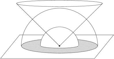
FIG. 9.: The “canonical” regularizing surface for the genus one case is a cone.

In the genus one case the space is the region between two hemispheres, the hemispheres being identified. In this case the desired family of regularizing surfaces consists of cones with the tip placed at $w=0$, see Fig. 9. As the angle $2\alpha$ at the tip of the cone increases $\alpha\to\pi/2$, the surface approaches the boundary. The metric induced on the surface of the cone is:

$$ds^{2}={l^{2}\over r^{2}\cos^{2}\alpha}\left(dr^{2}+r^{2}\sin^{2}\alpha d\phi^{2}\right),$$ (18)

and as $\alpha\to\pi/2$ this behaves as a diverging factor $(1/\cos^{2}\alpha)$ times the canonical torus metric, the torus coordinates being $\ln r/2\pi,\phi/2\pi$. Thus, this family of surfaces has the desired property that the induced metric approaches in the limit the canonical one. Note that this family of regularizing surfaces is the same as the one used in calculations of the black hole partition function [21, 43]. Indeed, the cones are just the spheres $r=const$ in the usual Schwarzschild-like coordinates. Let us now compute the regularized action. The volume of the region between the two hemispheres and inside the cone is given by:

$$V_{\alpha}=\pi l^{3}\left(\ln{\rho\over\rho^{\prime}}\right)\left({1\over\cos^{2}\alpha}-1\right).$$ (19)

The area of the part of the surface of the cone contained between the hemispheres is:

$$A_{\alpha}=2\pi l^{2}\left(\ln{\rho\over\rho^{\prime}}\right)\,{\sin\alpha\over\cos^{2}\alpha}.$$ (20)

Thus, the regularized action is:

$${V_{\alpha}\over 4\pi Gl^{2}}-{A_{\alpha}\over 8\pi Gl}={l\over 4G}\,\left(\ln{\rho\over\rho^{\prime}}\right)\,{1-\cos^{2}\alpha-\sin\alpha\over\cos^{2}\alpha},$$ (21)

which, in the limit $\alpha\to\pi/2$ gives

$$I=-{l\over 8G}\,\ln{\rho\over\rho^{\prime}}=-{l\over 8G}\,\ln|\lambda|\,,$$ (22)

where $\lambda$ is the multiplier of the transformation used to identify the hemispheres. This is the regularized action for the canonical metric on the torus. It is not hard to see that the result (22) reproduces correctly the free energy of AdS and BTZ spacetimes. For the case of periodically identified in the imaginary time AdS, $\ln|\lambda|$ is just the period $\beta$ of the imaginary time. Thus, for AdS:

$$I=-{\beta\over 8G},\qquad M={\partial I\over\partial\beta}=-{1\over 8G},$$ (23)

and the entropy is zero because the free energy depends linearly on $\beta$. In the case of the BTZ spacetime, $\ln|\lambda|$ is the horizon circumference $2\pi r_{+}$, and $\beta=2\pi l^{2}/r_{+}$. Thus,

$$I=-{1\over 8G}{(2\pi l)^{2}\over\beta},\qquad\qquad M={\partial I\over\partial\beta}={1\over 8G}{(2\pi l)^{2}\over\beta^{2}}={1\over 8G}{r_{+}^{2}\over l^{2}},$$ (24)

and

$$S=\beta M-I={1\over 4G}{(2\pi l)^{2}\over\beta}={2\pi r_{+}\over 4G},$$ (25)

which are the usual results for BTZ black hole.

We would now like to generalize the above calculation to the case of an arbitrary genus. The key problem here is to find a family of regularizing surfaces such that the induced metric approaches the canonical metric as the regulator is removed. This can be done using the solution to the Liouville equation, as we will show in III D. However, before we proceed with this construction, we need to review some relevant facts on Liouville theory.

C Uniformization. Liouville theory. Takhtajan-Zograf action.

Here we recall some facts about uniformization of Riemann surfaces by Kleinian groups, and the relation of this to Liouville theory. We shall also introduce the Takhtajan-Zograf action. The material reviewed here is from work [38].

One arrives at the Liouville equation considering the following problem. For each of the Riemann surfaces arising as the boundary of our spaces, we need to find the canonical curvature $R=-1$ metric that is in the same conformal class as the one induced by the flat metric. This is done as follows. Let us introduce complex coordinates $w$ on ${\bf S}$. The flat metric on ${\bf S}$ is $ds^{2}=|dw|^{2}$. The constant curvature metric we are looking for is related to the flat metric by a conformal transformation:

$$d\tilde{s}^{2}=e^{2\phi(w,\bar{w})}\,ds^{2}.$$ (26)

The field $\phi(w,\bar{w})$ is a real field on ${\bf S}$. The condition that $d\tilde{s}^{2}$ has constant curvature $R=-1$ then translates into an equation on $\phi$:

$$\Delta\phi=4\partial_{w}\partial_{\bar{w}}\phi={1\over 2}e^{2\phi}.$$ (27)

This is the famous Liouville equation. It is rather hard to solve in practice, except for the genus one case, but an indirect way of describing the solution is as follows. Let us recall that any Riemann surface $g>1$ can be uniformized by the upper half-plane $H$. This means, that, given a Riemann surface $X$, there is a projection map $\pi_{\Gamma}:H\to X$, which is just the quotient map of $H$ by the action of some (Fuchsian) discrete group $\Gamma$ of isomorphisms of $H$. Moreover, the group $\Gamma$ is isomorphic to the fundamental group $\pi_{1}(X)$. The Riemann surfaces $X$ arising in our construction are quotients of the complex plane ${\bf S}$. Let us uniformize them by the hyperbolic plane. We get a commutative diagram:

$$\diagram\node{H}\arrow[2]{e,t}{J}\arrow{se,b}{\pi_{\Gamma}}\node[2]{\Omega}\arrow{sw,r}{\pi_{\Sigma}}\\ \node[2]{X}$$ (28)

Here $\pi_{\Sigma}$ is the quotient map $\pi_{\Sigma}:\Omega\to\Omega/\Sigma=X$, where $\Sigma$ is the corresponding Schottky group. We are interested in the properties of the covering map $J:H\to\Omega$. The group of automorphisms of this map is isomorphic to the subgroup $N\subset\Gamma$, which is the smallest normal subgroup containing the elements $A_{i}\in\Gamma$. This map can be considered as a function on $H$, automorphic with respect to $A_{i}$, that is, $J\circ A_{i}=J$, and such that $J\circ B_{i}=L_{i}\circ J$. The inverse map $J^{-1}$ can be considered as a multi-valued function on ${\bf S}$. Let us denote by $z$ the complex coordinate on the hyperbolic plane $H$. Then the constant curvature $R=-1$ metric on $H$ is $|dz|^{2}/({\rm Im}z)^{2}$. We thus see, that, given the inverse map $J^{-1}$, the conformal factor mapping the flat metric $|dw|^{2}$ on ${\bf S}$ to the constant negative curvature metric on $H$ is:

$$e^{2\phi(w,\bar{w})}={|(J^{-1})^{\prime}(w)|^{2}\over({\rm Im}J^{-1}(w))^{2}},$$ (29)

where prime denotes the derivative with respect to $w$. It does not matter which branch of the function $J^{-1}$ is chosen. Thus, having constructed the uniformizing map $J$, we have the solution $\phi$ to the Liouville equation (27). From the above representation for $\phi$, it follows that it has the following transformation property:

$$\phi(Lw)=\phi(w)-{1\over 2}\,\ln{|L^{\prime}(w)|^{2}}.$$ (30)

It can be shown that there is a unique solution to the Liouville equation (27) on ${\bf S}$ with this transformation property. We also note, for further purposes, that the Liouville stress-energy tensor for $\phi$ is equal to the Schwarzian derivative of $J^{-1}$:

$$T_{w}=2\phi_{ww}-2\phi_{w}^{2}=\{J^{-1}(w);w\},$$ (31)

where $\{\cdot\,;\cdot\}$ is the Schwarzian derivative. This solution to the Liouville equation will be used in the next subsection to construct a “canonical” family of regularizing surfaces.

We will also need the action of Liouville theory on Riemann surfaces defined by Takhtajan and Zograf [38]. As before, a Riemann surface of genus $g$ is thought of as the quotient of the complex plane by the action of a Schottky group of genus $g$. The action of Takhtajan and Zograf is the following functional of the Liouville field:

$$I[\phi]=-{l\over 16\pi G}\left[\int\!\!\!\!\int_{D}{i\over 2}\,dw\wedge d\bar{w}\left(4\partial_{\omega}\phi\partial_{\bar{w}}\phi+{1\over 2}e^{2\phi}\right)+\right.$$ (32)

$$\left.i\sum_{i=2}^{g}\int_{C_{i}}\left(d\bar{w}\,\phi{\bar{L_{i}^{\prime\prime}}\over\bar{L_{i}^{\prime}}}-dw\,\phi{L_{i}^{\prime\prime}\over L_{i}^{\prime}}\right)-{1\over 2i}\sum_{i=2}^{g}\int_{C_{i}}\ln{|L_{i}^{\prime}|^{2}}\,{L_{i}^{\prime\prime}\over L_{i}^{\prime}}dw+4\pi\sum_{i=2}^{g}\ln{|l_{i}|^{2}}\right].$$ (33)

Here the first integral is taken over the fundamental region $D\subset{\bf S}$, which, in the case when the Schottky group is normalized, is the disc bounded by the circle $C_{1}$ minus the discs bounded by all other circles. The generators $L_{i}$ are thought of here as functions $L_{i}w$ on the complex plane. They can be represented in the normal form as:

$${L_{i}w-b_{i}\over L_{i}w-a_{i}}=\lambda_{i}{w-b_{i}\over w-a_{i}},\qquad|\lambda_{i}|>1.$$ (34)

Here $a_{i},b_{i}$ are the attracting and repelling fixed points of $L_{i}$, and $\lambda_{i}$ is the multiplier of the transformation. The quantity $l_{i}$ in the last term in (33) is the lower left corner matrix element of the matrix representation of $L_{i}$:

$$l_{i}={(\lambda_{i}-1)\over(a_{i}-b_{i})\sqrt{\lambda_{i}}}.$$ (35)

We use the anti-clockwise orientation of contours $C_{i},i>1$.

The action functional (33) has a number of important properties. First, the equation of motion that follows from it is just the Liouville equation. In fact, the first set of boundary terms in (33) is precisely such that its variation cancels the boundary terms arising in the variation of the “bulk” term, so that the variational principle is well-defined. Second, as one can explicitly check, by changing the position of one of the pair of circles $C,C^{\prime}$, the action (33) is independent of a choice of the fundamental region that was used to evaluate it. The second set of boundary terms is necessary for this property to hold. The last set of constants is precisely such that, when the action is evaluated on the solution to the Liouville equation, its variation with respect to the moduli gives the correct (Liouville) stress-energy tensor, see III E below. As we will demonstrate in the next subsection, the action (33) evaluated on the solution to the Liouville equation coincides with the regularized volume of the corresponding Euclidean space.

D “Canonical” regularization procedure

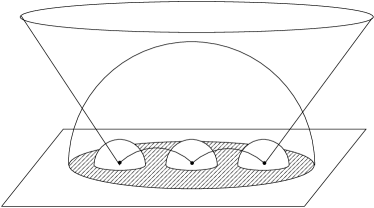
FIG. 10.: The “canonical” regularizing surface is constructed using the Liouville field.

In order to find the regularized action on the canonical metric, we need to find a family of regularizing surfaces such that the induced metric approaches the canonical one when the regulator is removed. To construct a desired family of regularizing surfaces we use the solution of the Liouville equation. To this end we use the Liouville field as the coordinate $z$ running orthogonally to the boundary, as suggested by the work of Polyakov [34] on non-critical string theory. More precisely, let us introduce a family of surfaces:

$$z(x,y)=\epsilon e^{-\phi(x,y)}.$$ (36)

The induced metric is then given by:

$$ds^{2}={l^{2}\over\epsilon^{2}}e^{2\phi}\left(dx^{2}+dy^{2}+\epsilon^{2}e^{-2\phi}\left({\partial\phi\over\partial x}dx+{\partial\phi\over\partial y}dy\right)^{2}\right).$$ (37)

As one can easily see, the induced metric behaves, when $\epsilon\to 0$, as $1/\epsilon^{2}$ times the canonical metric on the Riemann surface. A typical surface looks like the one shown in Fig. 10. It touches the boundary at points where the Liouville field diverges.

It is not hard to see that the prescription (36) generalizes the family of surfaces used in the genus one case. Indeed, in this case, the Liouville field can be found introducing the polar coordinates on ${\bf S}$ centered at $w=0$. Then the flat metric on the annulus is:

$$ds^{2}=|dw|^{2}=dr^{2}+r^{2}d\theta^{2}=e^{2\ln{2\pi r}}\left(\left({d\ln{r}\over 2\pi}\right)^{2}+\left({d\theta\over 2\pi}\right)^{2}\right).$$ (38)

Thus, after identifications are made, $\ln{r}/2\pi$ and $\theta/2\pi$ are coordinates on the torus, and $\phi=-\ln{2\pi r}=-\ln|2\pi w|$ is the Liouville field. We see that the family of surfaces (36) in this case is just the family of cones considered in III B.

Let us now use the regularizing surfaces (36) to compute the action. We would like to show that the regularized action, that is, the regularized volume contained in the region between the hemispheres and above the regularizing surface, in the limit when the regulator is removed, goes to the Liouville theory action (33) evaluated on the solution to the Liouville equation.

Before we go to the higher genus case, let us see how the action (33) reproduces the partition function for $g=1$. We notice that there are only contributions from the first term in (33). Indeed, in the genus one case, the term involving $e^{2\phi}$ is simply not there, because the Liouville equation in this case is just $\Delta\phi=0$. All other terms are zero because $L^{\prime\prime}=l=0$. Thus, evaluating the action on the Liouville field $\phi=-\ln 2\pi r$, we get:

$$I=-{l\over 16\pi G}\left[\int_{0}^{2\pi}d\theta\int_{\rho^{\prime}}^{\rho}rdr(1/r)^{2}\right]=-{l\over 8G}\ln|\lambda|,$$ (39)

which coincides with the expression for the partition function obtained before, see (22).

Let us now do the general case. The volume is given by:

$$V_{\epsilon}=l^{3}\int\!\!\!\!\int_{D_{1}^{\epsilon}}dxdy\int_{z_{\rm min}(x,y)}^{z_{\rm max}(x,y)}{dz\over z^{3}}\,,$$ (40)

where the $x,y$ integral is taken over the region $D_{1}^{\epsilon}$ inside the curve $C_{1}^{\epsilon}$, which is the projection on the $z=0$ plane of the curve along which the regularizing $\epsilon$-surface intersects the hemisphere built on the circle $C_{1}$. Thus, the points lying on $C_{1}^{\epsilon}$ satisfy the equation $z^{2}+|w|^{2}=\rho_{1}^{2}$. The upper limit of the integral over $z$ is:

$$z_{\rm max}(x,y)^{2}=\rho_{1}^{2}-(x^{2}+y^{2}).$$ (41)

The lower limit is different in different regions. We decompose

$$D_{1}^{\epsilon}=D^{\epsilon}\cup{D_{1}^{\epsilon}}^{\prime}\cup_{i=2}^{g}\left(D_{i}^{\epsilon}\cup{D_{i}^{\epsilon}}^{\prime}\right).$$ (42)

Within the region $D^{\epsilon}$ the lower integration limit is given by the regularizing surface. In all other regions it is given by the hemispheres built on $C_{1}^{\prime},C_{i},C_{i}^{\prime},i>1$. Thus, we have:

$$V_{\epsilon}=l^{3}\int\!\!\!\!\int_{D^{\epsilon}}dxdy{1\over 2\epsilon^{2}}e^{2\phi}-l^{3}\int\!\!\!\!\int_{D_{1}^{\epsilon}}{dxdy\over 2(\rho_{1}^{2}-(x^{2}+y^{2}))}+l^{3}\int\!\!\!\!\int_{{D_{1}^{\epsilon}}^{\prime}}{dxdy\over 2((\rho_{1}^{\prime})^{2}-(x^{2}+y^{2}))}$$ (43)

$$+l^{3}\sum_{i=2}^{g}\int\!\!\!\!\int_{D_{i}^{\epsilon}}{dxdy\over 2(\rho_{i}^{2}-((x-x_{i}^{0})^{2}+(y-y_{i}^{0})^{2}))}$$ (44)

$$+l^{3}\sum_{i=2}^{g}\int\!\!\!\!\int_{{D_{i}^{\epsilon}}^{\prime}}{dxdy\over 2((\rho_{i}^{\prime})^{2}-((x-{x_{i}^{0}}^{\prime})^{2}+(y-{y_{i}^{0}}^{\prime})^{2}))}\,.$$ (45)

Here $x_{i}^{0},y_{i}^{0}$ (and the corresponding primed quantities) are the coordinates of the center of the corresponding hemisphere. On the other hand, the area computed using the induced metric is equal to:

$$A_{\epsilon}=l^{2}\int\!\!\!\!\int_{D^{\epsilon}}dxdy{1\over\epsilon^{2}}e^{2\phi}\left(1+\epsilon^{2}e^{-2\phi}\left(\left({\partial\phi\over\partial x}\right)^{2}+\left({\partial\phi\over\partial y}\right)^{2}\right)\right)^{1/2},$$ (46)

which for $\epsilon\to 0$ behaves as:

$$A_{\epsilon}=l^{2}\int\!\!\!\!\int_{D^{\epsilon}}dxdy{1\over\epsilon^{2}}e^{2\phi}+{l^{2}\over 2}\int\!\!\!\!\int_{D^{\epsilon}}dxdy\left(\left({\partial\phi\over\partial x}\right)^{2}+\left({\partial\phi\over\partial y}\right)^{2}\right).$$ (47)

The first term here will cancel the first term on the right hand side of (44). The second term is just the kinetic term of the Liouville action (33). Let us compute the remaining terms on the right hand side of (44). They can be reduced to contour integrals by introducing the polar coordinates. The typical integral becomes:

$$\int_{0}^{2\pi}d\varphi\int_{0}^{r(\varphi)}{rdr\over 2(\rho_{i}^{2}-r^{2})}={1\over 4}\int_{0}^{2\pi}d\varphi\ln{\rho_{i}^{2}\over\rho_{i}^{2}-r^{2}(\varphi)}\,.$$ (48)

This can be further transformed by noticing that on the curve $C^{\epsilon}$ we have $\rho_{i}^{2}-r^{2}(\varphi)=\epsilon^{2}e^{-2\phi}$. Thus, the above integral reduces to:

$$l^{3}\pi\ln{\rho_{i}\over\epsilon}+{l^{3}\over 2}\int_{C_{i}^{\epsilon}}\phi,$$ (49)

where the last integral is the contour integral of the Liouville field. We should now remove the $\ln\epsilon$ divergence, combine all the pieces, and then remove the regulator. We get the correct “bulk” part of (33) plus a set of other terms:

$$I=({\rm``bulk^{\prime\prime}\,\,part})$$ (50)

$$-{l\over 16\pi G}\left(4\pi\ln{\rho_{1}\over\rho_{1}^{\prime}}-4\pi\ln{\rho_{2}\rho_{2}^{\prime}\cdots\rho_{g}\rho_{g}^{\prime}}+2\int_{C_{1}}\phi-2\int_{C_{1}^{\prime}}\phi-2\sum_{i=2}^{g}\int_{C_{i}}\phi-2\sum_{i=2}^{g}\int_{C_{i}^{\prime}}\phi\right).$$ (51)

This can be further simplified by using the transformation property (30) of $\phi$. The difference of the integrals over $C_{1},C_{1}^{\prime}$ then cancels the term proportional to $\ln{\rho_{1}/\rho_{1}^{\prime}}$, and we are left with:

$$I=({\rm``bulk^{\prime\prime}\,\,part})-{l\over 16\pi G}\left(-4\pi\ln{\rho_{2}\rho_{2}^{\prime}\cdots\rho_{g}\rho_{g}^{\prime}}-4\sum_{i=2}^{g}\int_{C_{i}}\phi+\sum_{i=2}^{g}\int_{C_{i}}\ln{|L_{i}^{\prime}|^{2}}\,\right).$$ (52)

The radii $\rho_{i}^{\prime}$ of the circles $C_{i}^{\prime}$ can be expressed through the radii $\rho_{i}$ and the parameters of the corresponding Schottky group generators. The radius $\rho_{i}^{\prime}$ of the circle $C_{i}^{\prime}=L_{i}(C_{i})$ is given by:

$$\rho_{i}^{\prime}={\rho_{i}\over|l_{i}|^{2}(\rho_{i}^{2}-|\xi_{i}-w_{i}^{0}|^{2})},$$ (53)

where $w_{i}^{0}$ is the center of the circle $C_{i}$, and $\xi_{i}$ is the pole of $L_{i}$ thought of as a function on the complex plane:

$$\xi_{i}={\lambda_{i}b_{i}-a_{i}\over\lambda_{i}-1}.$$ (54)

In order to compare (52) to the terms in the Takhtajan-Zograf action we notice that, the regularizing surfaces being chosen as in (36), the position and radii of the circles $C_{i},C_{i}^{\prime}$ cannot be chosen arbitrarily. Indeed, one has to make sure that, in the limit $\epsilon\to 0$, the circles $C_{i}^{\epsilon}$ are mapped into the circles ${C_{i}^{\epsilon}}^{\prime}$. As is not hard to see, the condition for this, for each pair of circles, is:

$${(\rho_{i}^{\prime})^{2}-|L_{i}w-{w_{i}^{0}}^{\prime}|^{2}\over|L_{i}^{\prime}|^{2}}=\rho_{i}^{2}-|w-w_{i}^{0}|^{2}.$$ (55)

Here $w_{i}^{0},{w_{i}^{0}}^{\prime}$ are the centers of circles $C_{i},C_{i}^{\prime}$ correspondingly. This can be satisfied for a special position of circles:

$$w_{i}^{0}={\lambda_{i}b_{i}-a_{i}\over\lambda_{i}-1}\,,\qquad{w_{i}^{0}}^{\prime}={\lambda_{i}a_{i}-b_{i}\over\lambda_{i}-1}\,.$$ (56)

For such position of the circles their radii $\rho_{i},\rho_{i}^{\prime}$ become equal. Thus, we have to compare (52) to the terms in (33) for this special choice of the position of circles. This is a simple exercise, for when the circles $C_{i}$ are centered as prescribed by (56), the function $\ln{|L_{i}^{\prime}|}$ is constant along $C_{i}$ (proportional to $\ln{\rho_{i}}$), and the calculation of all the contour integrals in (33) is straightforward. Performing this simple calculation one finds that (52) and (33) are equal.

A note is in order about the term involving $e^{2\phi}$ in the “bulk” part of (33). On-shell, this term is a constant, proportional to $2g-2$. Our regularization procedure, with the choice of the family of surfaces (36), does not reproduce this constant. One can get this term correctly by modifying the family of surfaces slightly. As is argued in [36], the correct relation between the Liouville field and the $z$ coordinate should involve the coupling to the boundary curvature $R$. Introducing such a coupling one can get the term involving $e^{2\phi}$ correctly. We shall not demonstrate this here. Instead, one can take another point of view that any regularization procedure is unavoidably ambiguous. The Takhtajan-Zograf action fixes this ambiguity of adding a constant to the action in a natural way.

The arguments presented show that the regularized volume computed using the above “canonical” family of regularizing surfaces is indeed given by the Takhtajan-Zograf action. Note that in order to use the simple family (36) of regularizing surfaces we had to place the circles $C_{i},C_{i}^{\prime}$ at special positions. One can presumably avoid doing this by modifying the regularizing family of surfaces appropriately, but we shall not try to perform this more general calculation. Note also that a part of the expression (50) that we obtained on an intermediate stage of our calculation is exactly the earlier result (17). Thus, one could also start from the result (17) and add to it the “bulk” Liouville action plus a collection of contour integrals adjusted so that the whole quantity renders the Liouville equations of motion under the variation. The total action can again be shown to be equal to the Takhtajan-Zograf action (33).

Having established that the regularized action for our spaces is given by the Liouville action evaluated on the “uniformizing” Liouville field, we can discuss properties of the boundary CFT.

E Stress-energy tensor.

Recall, see, e.g., [18], that the stress-energy tensor of a CFT can be thought of as a connection in a certain line bundle over the moduli space, this connection being compatible with a metric on the bundle, the role of the metric played by the partition function $Z$:

$$T=-Z^{-1}\partial Z,$$ (57)

where the derivative is taken with respect to the moduli. The regularized action $I$ is not yet (minus logarithm of) the partition function, the later can be obtained from $I$, in the semi-classical approximation, by summing over all solutions with the same conformal structure at infinity. However, it must be possible to interpret these solutions as the semi-classical states of the CFT; thus, the derivative of the free energy $I$ with respect to the moduli should have the interpretation of the stress-energy tensor for these states. The stress-energy tensor for each particular solution is also of direct importance in the thermodynamical considerations of the next subsection. It might also be of use in the problem of classification of solutions of (2+1)-gravity.

Thus, we would like to find the stress-energy tensor for each solution. By putting the action $I$ in the form (33) we achieved this goal, for the dependence of (33) on the moduli was studied in [38]. The Theorem 1 of [38], applied to the action (33), states that:

$${1\over 2}{\partial I\over\partial\omega_{i}}=-{l\over 16\pi G}c_{i},$$ (58)

where $\omega_{i}$ are the coordinates (3) on the Schottky space ${\mathfrak{S}}_{g}$, and $c_{i}$ are the coefficients in the decomposition of the Liouville stress-energy tensor $T_{w}$, or, the same, the Schwarzian derivative of the map $J^{-1}$, into the basis of quadratic differentials $P_{i}$ introduced in the Appendix.

We find the fact that the stress-energy tensor is given by the Schwarzian derivative of the uniformization map extremely appealing, for it has a nice CFT interpretation. Namely, in CFT one is used to the fact that, because of the presence of the conformal anomaly, the stress-energy tensor does not remain invariant under conformal transformations. More precisely, it is only invariant under the “global” conformal transformations, that is the ones mapping the complex sphere to itself, ${\rm SL}(2,{\mathbb{C}})$ transformations. However, in 2d any change of the complex coordinate on the worldsheet by an analytic function of it is a (locally) conformal transformation. Because of the conformal anomaly, the stress-energy tensor is not invariant under such more general transformations, and transforms by acquiring a multiple of the Schwarzian derivative of the map. These more general conformal transformations are the ones changing the global topology of the worldsheet. Thus, one can interpret the stress-energy tensor change under such a transformation as the Casimir energy “acquired” in the change of topology. The well-known example of this phenomenon is the Casimir energy of CFT on a cylinder, where it is given by the Schwarzian derivative of the map from the plane to the torus. More interesting example is given by the conformal dimension of the vacuum state in cyclic orbifold theories, which turns out to be the Schwarzian derivative of a map covering the cylinder $n$ times, see [8].

The boundary CFT we are discussing can also be thought as obtained by the orbifold construction. Indeed, all our Riemann surfaces are obtained from the complex plane by discrete identifications. Thus, one could think of some “mother” conformal field theory living on the plane, from which only certain states survive the identifications. Those states then are used to construct the partition function on a Riemann surface $X$. Then the vacuum state energy of the orbifolded CFT must be given by the Schwarzian derivative from the plane to $X$. Equation (58) shows this to be indeed the case.

It would definitely be of interest to calculate the stress-energy tensor, and parameters $c_{i}$ explicitly in some simple cases, as that of $g=2$. It would be even more interesting to find a relation between parameters $c_{i}$ and the mass and angular momentum parameters of the corresponding spacetimes. This would be interesting, for it would give an approach to the classification of solutions of (2+1) gravity with negative cosmological constant. Indeed, we saw that the corresponding Euclidean spaces are easy to classify by their boundaries, and then the dependence of their free energy $I$ on the moduli would allow one to find their mass and angular momentum parameters. We hope to develop such a classification scheme in the future.

F Thermodynamics.

We are now ready to study the thermodynamics of our spaces. The discussion in this subsection is mostly qualitative, for we were not able to explicitly calculate the action $I$ except in the genus one case. However, one can see the general picture even without knowing the action explicitly.

As we mentioned before, the regularized action $I$ has the meaning of the free energy of the corresponding space. As is clear from the construction leading to (33), it depends on the parameters of the Schottky groups generators, that is, it is a function on the Schottky space. Thus, the Schottky space ${\mathfrak{S}}_{g}$ should be interpreted as the space of allowed configurations (states) at genus $g$. As we saw in the previous subsection, deriving $I$ with respect to the coordinates $\omega_{i}$ on the Schottky space, we get components of the Liouville stress-energy tensor. This fact allows us to write the first law of thermodynamics for our spaces. Indeed, one has:

$$\delta I=\sum_{i=1}^{3g-3}{\partial I\over\partial\omega_{i}}\delta\omega_{i}=\sum_{i=1}^{3g-3}\left(-{lc_{i}\over 16\pi G}\right)\delta\omega_{i},$$ (59)

where we have used (58). Thus, the coordinates $\omega_{i}$ on the Schottky space play the role of intensive parameters, that is, they are analogs of temperature, pressure. On the other hand, the parameters $c_{i}$ play the role of extensive variables, such as energy, volume for usual systems. The equation (59) is then just the first law of thermodynamics written in terms of the free energy.

As we discussed in II B, our spaces have the interpretation of “Euclidean continuations” of black hole spacetimes. Such spacetimes have asymptotic regions, and thus are described by mass and angular momentum parameters for each asymptotic region. In addition, there are parameters describing the shape of the wormholes, hidden behind the horizons, or the relative position of the horizons with respect to one another, see [2] for more details. These parameters are of direct physical significance, but, in general, do not coincide with the parameters $c_{i}$, as well as the thermodynamically conjugate quantities $w_{i}$ do not coincide with temperatures, pressures etc. Thus, although the equation (59) has the interpretation of the first law, it is not the first law in the form involving the variations of the physical parameters. It would be quite desirable to find a relation between $\omega_{i}$ (or other known coordinates on the Schottky and Teichmuller spaces) and the physical parameters. One could then get a more informative form of the first law.

The problem of finding the physical parameters, such as the mass and angular momentum, in terms of the parameters $c_{i}$ is also directly related to the problem of finding the entropy of our spaces. Indeed, recall that the entropy of a “usual” thermodynamical system can be obtained from the free energy as: $S=\beta E-I$; there is no volume or pressure in this formula. Recall that all parameters describing our spaces can be divided into parameters describing the asymptotic regions, and the parameters specifying the “internal” geometry. The later ones are the analogs of pressure in the “usual” system. Thus, it is natural to define the entropy of a space under consideration as, schematically

$$S=\sum_{\vbox{\hbox{\rm asymptotic}\hbox{\,\,\,\,\,regions}}}\left(\beta E+\Phi J\right)-I,$$ (60)

where $\beta,\Phi$ are the conjugate variables to the energy $E$ and the angular momentum $J$; the sum is taken over all asymptotic regions. It would be quite desirable to try to define the physical parameters $E,J$ and their conjugate “intrinsically”, using only the geometrical properties of the Schottky (Teichmuller) space. This would then allow one to define the entropy function on the Teichmuller space. One expects this function to be equal to the quarter of the sum of the circumferences of all the horizons. Work is in progress to check whether this is indeed the case.

The thermodynamical stability of our spaces can also be discussed from the same general viewpoint. Recall that, in order to find whether a particular state is thermodynamically stable, one finds the matrix of specific heats at that state. If all of its eigenvalues are positive, the state is stable. To find the specific heat matrix for our spaces, we should derive the extensive parameters $c_{i}$ (“energies”) with respect to the intensive parameters $\omega_{i}$ (“temperatures”). This problem was solved in [38]. The Theorem 2 of this reference states:

$${\partial c_{i}\over\partial\bar{\omega}_{j}}=-{1\over 2}\langle{\partial\over\partial\omega_{i}}\,,\,{\partial\over\partial\omega_{j}}\rangle,$$ (61)

where $\langle\cdot\,,\,\cdot\rangle$ is the Weyl-Peterson metric on the Schottky (Teichmuller) space, reviewed in the Appendix. Thus, to analyze the thermodynamical stability of a particular state, one should just analyze the eigenvalues of the Weyl-Peterson metric at the corresponding point of the Schottky space. In general one should not expect the spaces considered to be “absolutely” stable, in the sense that all specific heats are positive. Indeed, the black hole spacetimes are, except in the simplest case of BTZ black hole, collapsing. One should, however, expect the asymptotic regions to be stable. Thus, at least the specific heats corresponding to the asymptotic regions must be positive.

Let us now turn to the question of phase transitions. As is well known, see [21], in asymptotically AdS spaces one has a phase transition (AdS at low temperatures) vs. (BH at high temperatures). In the context of AdS/CFT correspondence, this phase transition was interpreted in [43] as the phase transition in the boundary CFT. In the case of 2+1 dimensions, both periodically identified in the time direction AdS and the Euclidean black hole have the topology of the solid torus. Thus, the boundary has genus $g=1$. It is interesting whether one also gets phase transitions in the higher genus case. A simple argument shows that this must indeed be the case. Let us recall how one finds that there is a phase transition in the genus one case. Calculating the free energies of AdS and BTZ spaces, one finds that the free energy of AdS is the smallest of the two at small temperatures, while the free energy of BTZ is the smallest at large temperatures. The point where the two free energies are equal is the phase transition point. It is the point when the horizon radius of BTZ black hole is equal to the curvature radius of AdS: $r_{+}=l$. One can observe that AdS and the black hole spaces of the same temperature define the same conformal structure on the boundary. However, they realize different points in the Schottky space. As we discussed in II A, the Schottky space of the torus can be realized as the strip of the upper half-plane. Then AdS space and BTZ black hole of the same temperature are represented by two points on the imaginary axes related by the modular transformation $\tau\to-1/\tau$. The point where the phase transition occurs is the point where the free energies are equal, in other words, it is the point which is invariant under the above modular transformation. Thus, it is at points of the Schottky space which are invariant under some modular transformations that the free energies of different solutions are equal. At this point all such solutions are equally important; this is the point of a phase transition. Thus, one should expect phase transitions to occur at points of the Schottky space which are invariant under some modular transformations. These are exactly the points where the corresponding Riemann space has conical singularities. Such points exist not only in the genus one case, but also in the higher genus cases, where their pattern becomes much more complicated. It would be interesting to find these points for the case of $g=2$, and find which phase transitions they correspond to.

G Boundary CFT

We are now ready to study the boundary CFT partition function. The rules of bulk/boundary correspondence tell us that the semi-classical approximation to the partition function is given by the sum over all classical solutions which define the same conformal structure at the boundary. We saw that different classical solutions correspond to different points in the Schottky space. Two points that are related by a modular transformation correspond to the same conformal structure. Thus, to construct the partition function we have to take a sum over the action of the modular group on ${\mathfrak{S}}_{g}$ of the exponentials of (minus) the regularized action:

$$Z(\omega)=\sum_{\sigma\in{\rm Mod}({\bf S}_{g})}e^{-I[\sigma(\omega)]}.$$ (62)

Here the sum is taken over the elements $\sigma$ of the set ${\rm Mod}({\mathfrak{S}}_{g})$ of modular transformations of ${\mathfrak{S}}_{g}$. Recall that ${\rm Mod}({\mathfrak{S}}_{g})$ is the quotient of the group ${\rm Mod}(\Gamma)$ of all modular transformations by the normal subgroup consisting of those elements that send the group $N\subset\Gamma$ into itself. In (62), $\omega$ stands for the set of coordinates on the Schottky space ${\mathfrak{S}}_{g}$. Thus, assuming the sum in (62) converges, the partition function is a function on the Schottky space, which is by construction invariant under the modular transformations. It, therefore, descends to a function on the Riemann space. We note that the semi-classical approximation (62) to the partition function was studied, in the genus one case, in papers [29, 30, 14].

It is a good place to emphasize the role played in the whole construction by the Schottky space. As we see, the Schottky space is more important in our scheme than the Teichmuller space. It is different points in the Schottky space that correspond to different classical solutions. Points in the Teichmuller space that cover a particular point in ${\mathfrak{S}}_{g}$ just correspond to different choices of the basis of the generators $\alpha$ of $\pi_{1}(X)$. As we saw, the regularized action is a function on the Schottky space. It can be, of course, thought of as a function on Teichmuller space, but it will be invariant under the elements of ${\rm Mod}(\Gamma)$ that send $N\subset\Gamma$ to itself. A good analogy here is that a with gauge symmetry: the “gauge invariant” quantities only depend on a point in ${\mathfrak{S}}_{g}$, not on a point in its covering space $T_{g}$. This analogy also gives another point of view on why we sum in (62) over the modular transformations on ${\mathfrak{S}}_{g}$, not on $T_{g}$: it is usual in the path integral for a system with a gauge symmetry to sum only over the equivalence classes. To summarize, the Schottky space is more fundamental in our construction. In a sense, the Schottky space is the “reduced phase space”, while the Teichmuller space is the phase space where the gauge symmetry acts.

What is the CFT to whose partition function the expression (62) is an approximation? One possibility, suggested rather strongly by the role played in our story by the Liouville theory, is that this CFT is nothing else but the quantum Liouville theory. This theory is still far from being understood completely, despite some recent progress [35] on the subject, but the recent results seem to suggest that the theory does make sense quantum mechanically. If so, it would be extremely interesting to see in what regime the exact Liouville partition function is approximated by (62). Another possibility is that Liouville theory does not make sense quantum mechanically, or is not enough to account for all of the degrees of freedom expected to be found in (2+1)-dimensional quantum gravity. This would mean that there is no quantum theory of pure gravity in 2+1 dimensions (with negative cosmological constant). This possibility is advocated by some string theorists, see, e.g., [32]. If this turns out to be the case, one would only be able to interpret (62) as an approximation to the partition function of the CFT’s that arise in the context of AdS/CFT correspondence from string/M theory compactified on backgrounds containing AdS₃. These CFT’s are rather complicated, containing many fields. The expression (62) would then be interpreted as (an approximation to) the full generating functional, in which all the sources except for the stress-energy tensor source are put to zero.

We conclude this subsection by mentioning the possible orbifold interpretation of the CFT on higher genus surfaces. As we already discussed in III E, the semi-classical states of our theory (classical solutions) might be thought of as obtained from some “mother” conformal field theory on the plane by selecting states invariant under the discrete group $\Sigma$. The experience with orbifolds tells that one should expect the stress-energy for such states to be given by the Schwarzian derivative of the covering map. As we saw, the states considered have this property. It would be very interesting to develop this orbifold interpretation in more details.

IV Outlook

In this section we briefly discuss what our results imply for the problem of quantization of 2+1 gravity. Gravity in 2+1 dimensions is an extremely rich and beautiful theory. In the simplest case, when no matter is present and the space is compact, the theory is topological - its only degrees of freedom are global, topological properties of the underlying manifold. In this case it can be successfully quantized either canonically [40] or via recurse to Chern-Simons theory and its path integral [41]. This relates 2+1 gravity to such vast subjects as topological quantum field theory, knot theory, quantum groups. More complicated situations arise when one allows matter sources to be present. In fact, in this case one can get quite a non-trivial dynamics, in spite of the fact that there are no local degrees of freedom of the gravitational field itself. An example of such non-trivial dynamics, for the case when matter is just a collection of point particles, was exhibited in [25].

Another rich case is that of a negative cosmological constant, both with and without matter. In this case the space is not compact; one has asymptotic infinity with its rich structure. Simple arguments [10] based on semi-classical considerations show that quantum gravity in this case must be describable by some CFT living on the boundary. The old results of [13] suggest that this CFT is the to-be-constructed quantum Liouville theory. The results of [13], however, pertain only to the simplest boundary topology, that of $S^{1}\times{\mathbb{R}}$ in the Lorentzian case, or $S^{2}$ in the Euclidean regime. Our results for the general genus demonstrate it more convincingly that the boundary CFT must indeed be the Liouville theory.

We have already mentioned the point of view on the Schottky space as the “reduced phase space”, the “full phase space” being the Teichmuller space. In fact, this is more than an analogy. Asymptotic degrees of freedom of gravity with negative cosmological constant are the conformal structures one can put at infinity; thus, the Teichmuller space can indeed be thought of as the space of states of asymptotically AdS gravity. Moreover, both Teichmuller and Schottky spaces are symplectic manifolds, and thus are indeed phase spaces; the symplectic two-form is given by the imaginary part of the Weyl-Peterson hermitian metric. Thus, one can study the problem of quantization of these phase spaces. There is a growing body of evidence, see [39] and more recent papers [16, 26], that this quantum theory is nothing but the Liouville theory. What we found by studying the bulk/boundary correspondence also suggests that the boundary theory is the Liouville theory. This convergence of two different lines of thought is impressing.

If the boundary CFT is indeed the Liouville theory, then the bulk/boundary correspondence provides us with an interesting perspective on it. As is clear from our construction, the semi-classical states of the boundary CFT have the interpretation of classical solutions. The question then arises what spaces (spacetimes) in the bulk, if any, correspond to the “elementary” quantum states on the boundary. In fact, one may reverse the question and try to construct the quantum Liouville states as the ones corresponding to a particular nice set of spaces in the bulk. Such an approach to the quantum Liouville would be very much in the spirit of holography; it seems to be worth pursuing.

V Acknowledgments

I would like to thank A. Ashtekar, J. Baez, D. Brill, J. David, A. Hashimoto, K. Skenderis, J. Maldacena for discussions. I am grateful to L. Takhtajan and P. Zograf for correspondence. I am especially grateful to G. Horowitz for getting me interested in the subject as well as for discussions. This work was supported in part by NSF grant PHY95-07065.

A Teichmuller theory

Here we review some well-known facts on Teichmuller theory. Our presentation closely follows that of [38].

The space of possible conformal structures on a genus $g$ Riemann surface (the Riemann space) has a complicated structure, and it was the idea of Teichmuller to consider another, simpler space, out of which the Riemann space can be obtained as the quotient by a group of discrete transformations. The Teichmuller space is usually defined as the space of equivalence classes of quasiconformal mappings from a fixed base Riemann surface, see, e.g., [28]. However, in practice, it is more convenient to uniformize Riemann surfaces by Fuchsian groups, and consider the space of equivalence classes of Fuchsian groups obtained from a fixed, base Fuchsian group by quasiconformal transformations. The Teichmuller space so defined comes equipped with a coordinate system: these are the so-called Fricke coordinates, in which the Teichmuller space is a region in ${\mathbb{R}}^{6g-6}$.

Thus, let $\Gamma$ be a Fuchsian group uniformizing a marked Riemann surface $X$ of genus $g>1$. This Fuchsian group will serve as the base point. The Beltrami differential for $\Gamma$ is a complex-valued, bounded function $\mu$ on the unit disk $H$, having the property: $\mu(\gamma z)\overline{\gamma^{\prime}(z)}/\gamma^{\prime}(z)=\mu(z)$ for all $z\in H,\gamma\in\Gamma$. The vector space of all such functions will be denoted by $B(\Gamma)$. For every $\mu\in D(\Gamma)$, where $D(\Gamma)$ is the open unit ball (in the sense of the sup-norm) in $B(\Gamma)$, the Beltrami differential equation:

$$f^{\mu}_{\bar{z}}(z)=\mu(z)f^{\mu}_{z}(z)$$ (A1)

has a unique (up to transformations from ${\rm PSL}(2,{\mathbb{R}})$) solution in the class of quasiconformal maps of $H$ on itself. For every solution $f^{\mu}$, the group $\Gamma^{\mu}=f^{\mu}\Gamma(f^{\mu})^{-1}$ is a Fuchsian group uniformizing the Riemann surface that is obtained from $X$ as the result of the quasiconformal map $f^{\mu}$. Thus, every element $\mu\in D(\Gamma)$ gives a representation of $\Gamma$ in the group ${\rm PSL}(2,{\mathbb{R}})$: $\gamma\to f^{\mu}\gamma(f^{\mu})^{-1}$. The set of equivalence classes of such representations, where the equivalence is by inner automorphisms from of ${\rm PSL}(2,{\mathbb{R}})$, is called the Teichmuller space for $\Gamma$ and is denoted by $T(\Gamma)$. Let us note that choosing a different base point one obtains the same Teichmuller space. Thus, when the choice of the base point is not important, we will denote the Teichmuller space by $T_{g}$.

Thus, every Beltrami differential $\mu\in D(\Gamma)$ corresponds to a point in the Teichmuller space $T(\Gamma)$. Let us denote the corresponding map by $\Phi$:

$$\Phi:D(\Gamma)\to T(\Gamma).$$

Note that every Fuchsian group can be characterized by $6g$ parameters minus 3 relations (4). The equivalence classes are thus characterized by $6g-6$ parameters, this gives the so-called Fricke coordinates on the Teichmuller space. The Teichmuller modular group ${\rm Mod}(\Gamma)$ acts on $T(\Gamma)$ by discrete transformations, and the corresponding quotient space is the Riemann space: $R(\Gamma)=T(\Gamma)/{\rm Mod}(\Gamma)$.

Let us now introduce the so-called Weyl-Peterson metric on $T(\Gamma)$. First, we need a pairing between Beltrami differentials and holomorphic quadratic differentials. Let us define the space ${\cal Q}(\Gamma)$ of holomorphic quadratic differentials for group $\Gamma$ to be the space of holomorphic functions $q(z)$ on $H$ satisfying $q(\gamma z)\gamma^{\prime 2}(z)=q(z)$ for all $\gamma\in\Gamma,z\in H$. The Riemann-Roch theorem implies that ${\rm dim}_{\mathbb{C}}{\cal Q}(\Gamma)=3g-3$. We have a pairing:

$$(\mu,q)=\int\!\!\!\!\int_{H/\Gamma}\mu(z)q(z){|dz\wedge d\bar{z}|\over 2},$$ (A2)

which is invariantly defined because of the transformation properties of $\mu,q$. Let $N(\Gamma)\subset B(\Gamma)$ be the kernel of the above pairing. Then in every class $B(\Gamma)/N(\Gamma)$ there exists a representative of the form $({\rm Im}z)^{2}\overline{q(z)},q\in{\cal Q}(\Gamma)$. Such Beltrami differentials are called harmonic. The space of harmonic Beltrami differentials will be denoted by ${\cal H}(\Gamma)$.

The kernel of the differential $d\Phi$ of the map $\Phi:D(\Gamma)\to T(\Gamma)$ at point $\Phi(0)$ coincides with $N(\Gamma)$. Thus, the space ${\cal H}(\Gamma)$ can be identified with the tangent space to $T(\Gamma)$ at $\Phi(0)$. The pairing (A2) allows then to think of ${\cal Q}(\Gamma)$ as the cotangent space to $T(\Gamma)$ at $\Phi(0)$. The tangent and cotangent spaces at other points of $T(\Gamma)$ can be realized as ${\cal H}(\Gamma^{\mu}),{\cal Q}(\Gamma^{\mu})$.

One can now define a hermitian metric on $T(\Gamma)$:

$$\langle\mu_{1},\mu_{2}\rangle=(\mu_{1},({\rm Im}z)^{-2}\bar{\mu}_{2}),\qquad\mu_{1},\mu_{2}\in{\cal H}(\Gamma^{\mu}).$$ (A3)

This is the Weyl-Peterson metric. It is Kahler and invariant under ${\rm Mod}(\Gamma)$.

Let us now discuss a relation between the Teichmuller and Schottky spaces. As we discussed in II A, given a marked Riemann surface $X$, or, equivalently, a marked Fuchsian group $\Gamma$, one can construct the corresponding normalized marked Schottky group $\Sigma$. Thus, we have a map:

$$\Psi:T_{g}\to{\mathfrak{S}}_{g}\subset{\mathbb{C}}^{3g-3}.$$

The Teichmuller space is the universal covering space for ${\mathfrak{S}}_{g}$: the group of automorphisms of $\Psi$ is isomorphic to the fundamental group $\pi_{1}({\mathfrak{S}}_{g})$, and consists of those elements of ${\rm Mod}(\Gamma)$ that send the subgroup $N\subset\Gamma$ into itself.

Because ${\mathfrak{S}}_{g}$ is realized as a subspace of ${\mathbb{C}}^{3g-3}$, one has on it a preferred set of vector fields $\partial/\partial\omega_{i}$, where $\omega_{i},i=1,\ldots,3g-3$ are the coordinates (3) on the Schottky space. Using the map $\Psi$, they can be lifted to vector fields on $T_{g}$. The tangent bundle over $T_{g}$ is the space of holomorphic Beltrami differentials; one thus gets the basis of vector fields $\nu_{i}^{\mu}$ on $T_{g}$ that correspond to $\partial/\partial\omega_{i}$ on ${\mathfrak{S}}_{g}$:

$$d\Psi_{\Phi(\mu)}(\nu_{i}^{\mu})={\partial\over\partial\omega_{i}},\qquad\nu_{i}^{\mu}\in{\cal H}(\Gamma^{\mu}),i=1,\ldots,3g-3.$$ (A4)

One can then introduce the dual basis of quadratic differentials $p_{i}^{\mu},p_{i}^{\mu}\in{\cal Q}(\Gamma^{\mu})$. Let us also introduce the corresponding quadratic differentials $P_{i}^{\mu}$ on ${\bf S}$:

$$P_{i}^{\mu}=p_{i}^{\mu}\circ J_{\mu}^{-1}(J_{\mu}^{-1})^{\prime 2},$$ (A5)

where $J_{\mu}$ is the map from the hyperbolic plane $H$ to the region of discontinuity $\Omega_{\mu}$ of the Schottky group $\Sigma^{\mu}$ corresponding to $\Gamma^{\mu}$. The quadratic differentials $P_{i}^{\mu}$ are holomorphic functions of $\Omega_{\mu}$, automorphic with respect to $\Sigma^{\mu}$. The Schwarzian derivative of $J_{\mu}^{-1}$, which is a holomorphic quadratic differential on $\Omega_{\mu}$, can be decomposed into the basis of $P_{i}^{\mu}$:

$$\{J_{\mu}^{-1}(w);w\}=\sum_{i=1}^{3g-3}c_{i}^{\mu}P_{i}^{\mu}(w).$$ (A6)

The quantities $c_{i}$ are functions on the Schottky space: $c_{i}^{\mu}$ depends on the parameters of the Schottky group $\Sigma^{\mu}$. As we show in III F, they play the role of the extensive thermodynamical parameters for our spaces, while the coordinates $\omega_{i}$ on the Schottky space are the intensive parameters.

REFERENCES

- [1] O. Aharony, S.S. Gubser, J. Maldacena, H. Ooguri, Y. Oz, Large N field theories, string theory and gravity, hep-th/9905111.
- [2] S. Aminneborg, I. Bengtsson, D. Brill, S. Holst, P. Peldan, Black holes and wormholes in (2+1)-dimensions, Class. Quant. Grav. 15 627-644 (1998). See also: D. Brill, Black holes and wormholes in (2+1)-dimensions, gr-qc/9904083.
- [3] S. Aminneborg, I. Bengtson, S. Holst, A spinning anti-de Sitter wormhole, Class. Quant. Grav. 16 363-382 (1999).
- [4] V. Balasubramanyan and P. Kraus, A stress tensor for anti-de Sitter gravity, Comm. Math. Phys. 208 413-428 (1999).
-
[5]
K. Bautier, Diffeomorphisms and Weyl transformations
in AdS3 gravity,
hep-th/9910134. - [6] D. Birmingham, C. Kennedy, S. Sen, A. Wilkins, Geometrical finiteness, holography and the BTZ black hole, Phys. Rev. Lett. 82 4164-4167 (1999).
- [7] G. Bonelli, Holography and CFT on generic manifolds, Phys. Lett. B450 363-367 (1999).
- [8] L. Borisov, M.B. Halpern, C. Schweigert, Systematic approach to cyclic orbifolds, Int. J. Mod. Phys. A13 125-168 (1998).
- [9] D. Brill, (2+1)-dimensional black holes with momentum and angular momentum, gr-qc/9912079.
- [10] J.D. Brown and M. Henneaux, Central charges in the canonical realization of asymptotic symmetries: an example from three-dimensional gravity, Comm. Math. Phys. 104 207-226 (1986).
- [11] S. Carlip and C. Teitelboim, Aspects of black hole quantum mechanics and thermodynamics in (2+1)-dimensions, Phys. Rev. D51 622-631 (1995).
- [12] L. Chekhov, AdS3/CFT2 correspondence at finite temperature, Mod. Phys. Lett. A14 2157-2168 (1999).
- [13] O. Coussaert, M. Henneaux, P. van Driel, Asymptotic dynamics of three-dimensional Einstein gravity with a negative cosmological constant, Class. Quant. Grav. 12 2961-2966 (1995).
- [14] R. Dijkgraaf, J. Maldacena, G. Moore and E. Verlinde, A black hole farey tale, hep-th/0005003.
- [15] W. Fenchel, Elementary geometry in hyperbolic space, de Gruyter, Berlin, 1989.
- [16] V.V. Fock, Dual Teichmuller spaces, dg-ga/9702018; L. Chekhov and V.V. Fock, Quantum Teichmuller space, math/9908165.
- [17] L. Ford, Automorphic functions, Chelsea Pub. Co., New York, 1972.
- [18] D. Friedan and S. Shenker, The analytic geometry of two-dimensional conformal field theory, Nucl. Phys. B281 509 (1987).
- [19] S. Gubser, I. Klebanov and A.M. Polyakov, Gauge theory correlators from noncritical string theory, Phys. Lett. B428 105-114 (1998).
- [20] S. Hamidi and C. Vafa, Interactions on orbifolds, Nucl. Phys. B279 456 (1987).
- [21] S. Hawking and D. Page, Thermodynamics of black holes in anti de-Sitter space, Comm. Math. Phys. 87 577 (1983)
- [22] D. Hejhal, On Schottky and Teichmuller spaces, Adv. in Math. 15 133-156 (1975).
- [23] M. Henningson and K. Skenderis, The holographic Weyl anomaly, JHEP 9807 023 (1998).
- [24] S. Holst and H.-J. Matschull, The anti-de Sitter Gott universe: a rotating BTZ wormhole, Class. Quant. Grav. 16 3095-3131 (1999).
- [25] G. ’t Hooft, Causality in 2+1 dimensions, Class. Quant. Grav. 9 1335-1348 (1992).
- [26] R.M. Kashaev, Quantization of Teichmuller spaces and the quantum dilogarithm, q-alg/9705021; Liouville central charge in quantum Teichmuller theory, hep-th/9811203.
- [27] A. Kholodenko, Boundary conformal field theories, limit sets of Kleinian groups and Holography, hep-th/9902167.
- [28] O. Lehto, Univalent functions and Teichmuller spaces, Springer-Verlag, New York, 1987.
- [29] J. Maldacena and A. Strominger, AdS3 black holes and a stringy exclusion principle, J. High Energy Phys. 9812 005 (1998).
- [30] S. Mano, AdS3 gravitational instantons from conformal field theory, Mod. Phys. Lett. A14 1961-1982 (1999).
- [31] D. Marolf and G. Horowitz, A new approach to string cosmology, JHEP 9807 014 (1998).
- [32] E. Martinec, Conformal field theory, geometry, and entropy, hep-th/9809021.
- [33] B. Maskit, Kleinian groups, Springer-Verlag, New York, 1988.
- [34] A. Polyakov, String theory and quark confinement, Nucl. Phys. Proc. Suppl. 68 1-8 (1998).
- [35] B. Ponsot and J. Teschner, Liouville bootstrap via harmonic analysis on a non-compact quantum group, hep-th/9911110.
- [36] N. Seiberg and E. Witten, The D1/D5 system and singular CFT, JHEP 9904 017 (1999).
- [37] K. Skenderis and S. Solodukhin, Quantum effective action from the AdS/CFT correspondence, Phys. Lett. B472 316-322 (2000).
- [38] L. Takhtajan and P. Zograf, On uniformization of Riemann surfaces and the Weyl-Peterson metric on Teichmuller and Schottky spaces, Math. USSR Sbornik 60 297-313 (1988).
- [39] H. Verlinde, Conformal field theory, two-dimensional quantum gravity and quantization of Teichmuller space, Nucl. Phys. B337 652-680 (1990).
- [40] E. Witten, 2+1 dimensional gravity as an exactly solvable system, Nucl. Phys. B311 46-78 (1988).
- [41] E. Witten, Quantum field theory and the Jones polynomial, Comm. Math. Phys. 121 351 (1989).
- [42] E. Witten, Anti-de Sitter space and holography, Adv. Theor. Math. Phys. 2 253-291 (1998).
- [43] E. Witten, Anti de-Sitter space, thermal phase transition, and confinement in gauge theories, Adv. Theor. Math. Phys. 2 505-532 (1998).
- [44] E. Witten and S. T. Yau, Connectedness of the boundary in the AdS/CFT correspondence, hep-th/9910245.
- [45] P. G. Zograf, The Liouville action on moduli spaces and uniformization of degenerating Riemann surfaces, Leningrad Math. J. 1 941 (1990).