Crossing probabilities on same-spin clusters
in the two-dimensional Ising model

Abstract

Probabilities of crossing on same-spin clusters, seen as order parameters, have been introduced recently for the critical 2d Ising model by Langlands, Lewis and Saint-Aubin. We extend Cardy’s ideas, introduced for percolation, to obtain an ordinary differential equation of order $6$ for the horizontal crossing probability $\pi_{h}$. Due to the identity $\pi_{h}(r)+\pi_{h}(1/r)=1$, the function $\pi_{h}$ must lie in a 3-dimensional subspace. New measurements of $\pi_{h}$ are made for $40$ values of the aspect ratio $r$ ($r\in[0.1443,6.928]$). These data are more precise than those obtained by Langlands et al as the $95$%-confidence interval is brought to $4\times 10^{-4}$. A $3$-parameter fit using these new data determines the solution of the differential equation. The largest gap between this solution and the 40 data is smaller than $4\times 10^{-4}$. The probability $\pi_{hv}$ of simultaneous horizontal and vertical crossings is also treated.

Les probabilités de traversée sur les plages de spins identiques, vues comme paramètres d’ordre, ont été introduites récemment pour le modèle d’Ising bidimensionnel critique par Langlands, Lewis et Saint-Aubin. Nous étendons les idées de Cardy, présentées pour la percolation, afin d’obtenir une équation différentielle ordinaire du sixième ordre pour la probabilité d’une traversée horizontale $\pi_{h}$. Il suit de l’identité $\pi_{h}(r)+\pi_{h}(1/r)=1$ que $\pi_{h}$ doit reposer dans un sous-espace de dimension trois. De nouvelles mesures de $\pi_{h}$ sont faites pour $40$ valeurs du rapport $r$ des côtés du rectangle ($r\in[0.1443,6.928]$). L’intervalle de confiance de $95$% est ici réduit à $4\times 10^{-4}$. La solution de l’équation différentielle est choisie en minimisant l’écart quadratique entre la solution et ces nouvelle données. Le plus grand écart entre les données et la solution ainsi obtenue est plus petit que $4\times 10^{-4}$. La probabilité de traversées horizontale et verticale simultanées est également étudiée.

Short Title: Crossing probabilities in the 2d Ising model

PACS numbers: 0.50.+q, 64.60.Fr, 64.60.Ak, 11.25.Hf

1 Introduction

The probability $\pi_{h}(r)$ of crossing on open sites inside a rectangle of aspect ratio $r$ has been measured at $p_{c}$ for several models of percolation in [6] and [7]. These simulations support hypotheses of universality and conformal invariance of this function $\pi_{h}(r)$ and of several others. Cardy’s contemporaneous work [1] offered a prediction for $\pi_{h}$ using conformal field theory. His analytic expression agrees with the simulations within statistical errors and provides further support that these crossing probabilities are order parameters with the usual critical properties.

This paper presents similar evidence, both numerical and analytic, for crossing probabilities on same-spin clusters of the two-dimensional Ising model at criticality. These crossing probabilities are not traditional order parameters for the Ising model. It is not a priori obvious that they are not identically zero or one in any dimension $d$. In dimension two however the simulations carried out in [5] indicates clearly that they are non-trivial functions and that they are likely to satisfy the same hypotheses (or even more restrictive ones) of universality and conformal invariance. Moreover physical quantities for which conformal field theory gives quantitative predictions that can be readily verified by simulation are always welcome.

Let a triangular lattice be oriented in such a way that sites on horizontal lines are at a distance of one mesh unit. A rectangle of height $V$ and width $H$ is superimposed on the lattice. The width $H$ is measured in mesh units but $V$ is the number of horizontal lines in the rectangle. A configuration of the Ising model has a horizontal crossing if there exists a path made of edges between nearest neighbor sites going from the leftmost inner column to the rightmost one and visiting only plus spins. (Because of the relative position of the rectangle and the lattice, the vertical columns are made of sites in zigzag.) Let $\pi_{h}(V,H)$ be the probability at the critical temperature of such a crossing. One defines similarly a vertical crossing and the associated probability $\pi_{v}(V,H)$. It is a well-known fact from percolation theory that, on the triangular lattice, a horizontal crossing on plus spins (or open sites) exist if and only if there is no vertical crossing on minus spins (closed sites). (One can convince oneself easily of this simple fact using a drawing.) Since plus and minus spins are equiprobable, this observation implies $\pi_{h}(V,H)+\pi_{v}(V,H)=1$. In this paper we will ultimately be interested in the limit $\pi_{h}(r)=\lim_{V,H\rightarrow\infty,r=\sqrt{3}V/2H}\pi_{h}(V,H)$ and similarly for $\pi_{v}$. The infinite lattice limit of the previous relation is known as the duality relation: $\pi_{h}(r)+\pi_{v}(r)=1$. If $\pi_{h}$ and $\pi_{v}$ are rotational invariants, the latter relation can be written as $\pi_{h}(r)+\pi_{h}(1/r)=1$. This duality relation will hold for other (regular) lattices if the functions $\pi_{h}$ and $\pi_{v}$ are universal but its discrete equivalent ($\pi_{h}(V,H)+\pi_{v}(V,H)=1$) hold strictly for neither the square nor the hexagonal lattices.

The present paper discusses both a prediction for $\pi_{h}$ extending Cardy’s approach and precise measurements of the function $\pi_{h}$ for $40$ values of its parameter $r$. The agreement will be seen to be excellent, that is, perfect within statistical errors. The first section covers the theoretical prediction, the second the details of the simulation and the comparison of the data with the prediction.

2 A theoretical prediction based
on conformal field theory

2.1 Cardy’s prediction for percolation

Cardy’s prediction for $\pi_{h}$ for two-dimensional percolation proceeds in two steps. He first identifies the probability $\pi_{h}$ with the difference of two partition functions with boundary conditions for the $1$-state Potts model. He then uses the conformal field theory at $c=0$ to obtain an analytic expression for this difference. Here is a (very rapid) presentation of these two steps.

The partition function $Z(q)$ of the $q$-state Potts model on a finite rectangular domain is the sum over all configurations $\sigma$ of $e^{-\beta H(\sigma)}$ where $H(\sigma)=J\sum_{\langle x,y\rangle}(1-\delta_{\sigma(x),\sigma(y)})$. The sum in $H(\sigma)$ runs over immediate neighbor pairs $\langle x,y\rangle$. This can be rewritten as $Z(q)=\sum_{R}p^{B(R)}(1-p)^{B-B(R)}q^{N_{c}(R)}$ where $p=1-e^{-\beta J}$. The sum is over all subsets $R$ of the set of edges of the lattice in the rectangular domain. The integer $B$ counts the edges in the lattice, $B(R)$ those in the subset $R$ and $N_{c}(R)$ the clusters in $R$. If $q=1$ (the value for percolation), this sum is 1 as desired. Let $Z_{\alpha\beta}$ be the partition function of the Potts model for configurations whose spins on the left side of the rectangle are in the state $\alpha\in\{1,2,\dots,q\}$, those on the right in the state $\beta$, and the others free. Cardy’s first crucial observation is that $\pi_{h}=\left.(Z_{\alpha\alpha}-Z_{\alpha\beta})\right|_{q=1}$ where $\alpha\neq\beta$. (The difference, done for a “generic” $q$, contains precisely the configurations that have a cluster intersecting the left and right sides.) The problem of calculating $\pi_{h}$ is therefore transformed into that of calculating partition functions.

The possibility of calculating partition functions on finite domains with given boundary conditions also originates from works by Cardy (see for example [2]). In the case of $Z_{\alpha\beta}$, for example, the four sides of the rectangle are submitted respectively to the boundary conditions $\alpha$, free, $\beta$ and free. Cardy argues that such a partition function is proportional to the $4$-point correlation function $\langle\phi(z_{1})\phi(z_{2})\phi(z_{3})\phi(z_{4})\rangle$ in the conformal field theory associated to percolation whose central charge is $c=0$. The $z_{i}\in\mathbb{C}$ are the vertices of the rectangle in the complex plane and $\phi$ is the field that changes the boundary conditions in this theory. For percolation, this field is identified to $\phi_{1,2}$ and it has conformal weight $h=0$, a necessary condition for $\langle\phi(z_{1})\phi(z_{2})\phi(z_{3})\phi(z_{4})\rangle$ to be scale invariant. (The indices on $\phi_{1,2}$ refer to the labels of Kac table. See [3].) The rules to find correlation functions in a conformal field theory are well-known and with this identification between partition functions with boundary conditions and $4$-point correlation functions, the problem of calculating $\pi_{h}$ amounts to solving an ordinary differential equation.

Two obstacles appear in applying these ideas to the Ising model. First the Ising model is the $q=2$ Potts model and the difference $(Z_{\alpha\alpha}-Z_{\alpha\beta})|_{q=2}$ cannot be interpreted as the crossing probability since the factor $q^{N_{c}(R)}$ in the sum gives different weights to the various configurations that have a crossing from left to right. Second although the operator for the Ising model that changes the boundary state from free to a given state $\alpha$ is still $\phi_{1,2}$, as in percolation, its conformal weight $h_{1,2}$ is now $\frac{1}{16}$ and its $4$-point correlation is not anymore invariant under a conformal mapping $z\rightarrow w$ but picks up the usual jacobian factors: $\langle\phi(w_{1})\phi(w_{2})\phi(w_{3})\phi(w_{4})\rangle=(\prod_{i}|w^{\prime}(z_{i})|^{-h_{1,2}})\langle\phi(z_{1})\phi(z_{2})\phi(z_{3})\phi(z_{4})\rangle$. These prefactors (and those additional coming from the presence of vertices along the boundary) seem to contradict the (strict) conformal invariance observed by simulation in [5].

In [6] and [7] the probability $\pi_{hv}$ of having simultaneous horizontal and vertical crossings was also obtained numerically. Watts [8] was able to extend Cardy’s argument to obtain a prediction that fits extremely well the data. His work is of particular interest to us as he is able to write $\pi_{hv}$ again as a partition function but with more general boundary conditions. Whether a conformal boundary operator accomplishes the change between these more complex boundary conditions is not clear. Nonetheless the expression of $\pi_{hv}$ as a partition function allows us to expect, Watts argues, that this probability is given by some $4$-point correlation function. He seeks it in the $h=0$ sector.

2.2 The differential equation for $\pi_{h}$

Cardy’s argument for percolation cannot be extended to the Ising model. One can still hope to relate crossing probabilities like $\pi_{h}$ to $4$-point correlation functions as Watts did for $\pi_{hv}$ of percolation. If such a relationship exists, the choice can be narrowed to $4$-point functions of the identity family as these are the only ones in the $c=\frac{1}{2}$ conformal field theory that are invariant under conformal map $z\rightarrow w$ like $\pi_{h}(r)$. An obvious objection will be that the $4$-point function of the primary field in the identity family is identically $1$ (or a constant). For the calculation at hand it might well be that this primary field must be interpreted as one whose correlation functions satisfy only one of the differential equations corresponding to the two leading singular vectors. This milder requirement does not force the function to be a constant as will be seen immediately.

The Verma module $V_{(c=\frac{1}{2},h=0)}$ of the Virasoro algebra has a maximal proper submodule $M$ generated by two singular vectors, one at level $1$, the other at level $6$. The first of these is $L_{-1}|0\rangle$ and the corresponding differential equation implies that the $4$-point function is a constant. We shall drop this requirement. The other singular vector is

$$\left({L_{{-1}}}^{6}-10\,{L_{{-1}}}^{4}L_{{-2}}+{\frac{43}{3}}\,{L_{{-1}}}^{2}{L_{{-2}}}^{2}-{\frac{100}{27}}\,{L_{{-2}}}^{3}+{\frac{97}{2}}\,{L_{{-1}}}^{3}L_{{-3}}\right.$$

$$-{\frac{337}{6}}\,L_{{-1}}L_{{-2}}L_{{-3}}+{\frac{3185}{144}}\,{L_{{-3}}}^{2}-{\frac{381}{2}}\,{L_{{-1}}}^{2}L_{{-4}}+{\frac{1265}{18}}\,L_{{-2}}L_{{-4}}$$

$$\left.+{\frac{19309}{36}}\,L_{{-1}}L_{{-5}}-{\frac{9005}{12}}\,L_{{-6}}\right)\left|c={\textstyle{\frac{1}{2}}},h=0\right\rangle.$$

If $f(z)$ is the $4$-point function with $z=(z_{1}-z_{2})(z_{3}-z_{4})/(z_{1}-z_{3})(z_{2}-z_{4})$, the differential equation is

$$\begin{split}{\frac{1}{72}}\,\left(1-2\,z\right)\left(686\,{z}^{2}\left(1-z\right)^{2}+73\,z\left(1-z\right)+25\right){\frac{d}{dz}}f(z)&\\ +{\frac{1}{144}}\,z\left(1-z\right)\left(25141\,{z}^{2}\left(1-z\right)^{2}-2986\,z\left(1-z\right)-171\right){\frac{d^{2}}{d{z}^{2}}}f(z)&\\ +\frac{1}{27}\,{z}^{2}\left(1-z\right)^{2}\left(1-2\,z\right)\left(208-3595\,z\left(1-z\right)\right){\frac{d^{3}}{d{z}^{3}}}f(z)&\\ +\frac{1}{6}\,{z}^{3}\left(1-z\right)^{3}\left(137-737\,z\left(1-z\right)\right){\frac{d^{4}}{d{z}^{4}}}f(z)&\\ +10\,\left(1-2\,z\right){z}^{4}\left(1-z\right)^{4}{\frac{d^{5}}{d{z}^{5}}}f(z)&\\ +{z}^{5}\left(1-z\right)^{5}{\frac{d^{6}}{d{z}^{6}}}f(z)&=0.\end{split}$$ (1)

This differential equation has three (regular) singular points at $0,1$ and $\infty$. It is invariant under any permutation of these three points. (Invariance under $z\rightarrow 1-z$ is clear: invariance under $z\rightarrow 1/z$ requires some work.) The exponents at any of these points are $0$, $\frac{1}{6}$ twice degenerate, $\frac{1}{2}$, $\frac{5}{3}$ and $\frac{5}{2}$. The monodromy matrices around the three singular points are similar due to the symmetry of the equation but they cannot be diagonalized simultaneously.

The cross-ratio $z=(z_{1}-z_{2})(z_{3}-z_{4})/(z_{1}-z_{3})(z_{2}-z_{4})$ is related to the aspect ratio $r=\sqrt{3}V/2H$ of the rectangle. If the four points $z_{1},z_{2},z_{3}$ and $z_{4}$ are chosen along the real axis at $-\frac{1}{k},-1,1,\frac{1}{k}$, then

$$k=\frac{1-\sqrt{z}}{1+\sqrt{z}}.$$

A Schwarz-Christoffel transformation can be used to map the upper plane onto a rectangle with the images of the $z_{i}$ at the vertices. The aspect ratio is then given as

$$r=\frac{K(1-k^{2})}{2K(k^{2})}$$

where $K$ is the complete elliptic integral of the first kind. The very short but wide rectangles ($r=\sqrt{3}V/2H\rightarrow 0^{+}$) corresponds to $z\rightarrow 0^{+}$, the tall and narrow ($r\rightarrow+\infty$) to $z\rightarrow 1^{-}$ and the square to $r=1,z=\frac{1}{2}$. The function $r(z)$ has the property $r(z)=r(\frac{1}{z})$ and the symmetry $z\rightarrow\frac{1}{z}$ of the differential equation is thus welcome. If $\pi_{h}$ does not depend on the relative angle between the rectangle and the lattice, that is if $\pi_{h}$ is a rotational invariant, then the duality relation implies $\pi_{h}(1)=\frac{1}{2}$ and it can be put in the form $(\frac{1}{2}-\pi_{h}(r))=-(\frac{1}{2}-\pi_{h}(\frac{1}{r}))$. Fortunately the function $r(z)$ is such that $r(z)=1/r(1-z)$ and the duality simply states that the function $f(z)=\frac{1}{2}-\pi_{h}(r(z))$ is odd with respect to the axis $z=\frac{1}{2}$. An odd subspace of the solution space of the differential equation (odd with respect with $z=\frac{1}{2}$) exists due to the symmetry $z\rightarrow 1-z$ and it is of dimension $3$.

We explored several paths to cast the solutions of eq. (1) into analytically tractable forms. One of them was to write the lhs of eq. (1) as $\prod_{1\leq i\leq 6}(z(1-z))^{a_{i}}\frac{d}{dz}$ like Watts did. But there is no real solutions for the $a_{i}$’s in the present case. The most natural path however is the screening operator method ([4], see also [3]). The pertinent field is $\phi_{2,3}$ (with Kac’s labels) and the 4-point correlation calls for three contour integrals (a charge $Q_{+}Q_{-}^{2}$ must be added at infinity to assure neutrality). Integral representations of six linearly independent solutions can be obtained in this straightforward (but probably tedious) way. The main problem is therefore whether there is sufficient physical information on $f$ to fix the linear combination. As argued above the odd parity of $f$ reduces the space of solutions to a three-dimensional subspace. The condition $f(0)=-\frac{1}{2}$ (i.e. $\pi_{h}(0)=1-\pi_{h}(1)=0$) is one further linear constraint. The function $f(z)$ is monotone increasing but this condition will restrict $f$ to an open set of the $3$-d subspace rather than decrease the dimension. The numerical data presented below indicate that $\pi_{h}(z)\rightarrow z^{\frac{1}{6}}$ as $z\rightarrow 0^{+}$. This is rather striking in view of the two-fold degeneracy of the exponent $\frac{1}{6}$. Two solutions associated to this exponent can be chosen to behave as $z^{\frac{1}{6}}$ and $z^{\frac{1}{6}}\log z$ for small $z$ and the latter, if present in $f$, should dominate the former whenever $z$ is close to $0$. The fact that it is not seen in the simulation could be interpreted physically as a manifestation of the power law behavior of critical correlation functions at short distance. Imposing that the behavior in $z^{\frac{1}{6}}\log z$ be absent of $f$ would add one linear constraint. With all these constraints we would still be left with a one-dimensional subspace in the space of odd solutions. We have not found any further constraints to fix completely the function $f$. This is why we resorted to a numerical fit (see Paragraph 3.2).

As we were trying to solve analytically the differential equation, Marc-André Lewis suggested to us to look for a solution of the form $ez^{d}{}_{2}F_{1}(a,b,c;z)$, with $a,b,c,d$ and $e$ constants, that would be odd around $z=\frac{1}{2}$ and reproduce the asymptotic behavior of the data. Cardy’s prediction for percolation is of this form and the suggestion is natural in this sense. Such a function exists but it does not satisfy the differential equation. However it follows so closely the data of [5] (the worst gap is $1$%) that we decided to improve these measurements to answer the question: which of the hypergeometric function or of the solution of the differential equation, if any, describes the data.

3 Improved measurements of $\pi_{h}$

3.1 Finite size effects and power law behavior

The probabilities $\pi_{h},\pi_{v}$ and $\pi_{hv}$ at $81$ values of $r$ ($\in[0.136,7.351]$) were measured in [5] for the three regular lattices on rectangles containing around $40000$ sites. For these sizes, departure from the duality relation is small but still noticeable for the square and the hexagonal lattices. No attempt was made there to use various sizes in order to reduce finite-size effects. For the new runs to be presented here we chose to concentrate on the triangular lattice and use various sizes to approximate the function $\pi_{h}$ (and the other two, $\pi_{v}$ and $\pi_{hv}$) in the limit when the mesh goes to zero.

A power law for the finite-size behavior of critical data is an accepted hypothesis and our measurements rest upon it. It states that, for sufficiently large size,

$$|\pi_{h}(V,H)-\pi_{h}(r)|\approx aV^{\beta}$$

with $\beta$ a negative constant and $r=\sqrt{3}V/2H$. We shall use several linear sizes of the form $V=2^{i}V_{0}$ and $H=2^{i}H_{0}$. Writing $\pi_{h}(i)$ for $\pi_{h}(2^{i}V_{0},2^{i}H_{0})$ and supposing that $\pi_{h}(i)$ is decreasing, we can write $\pi_{h}(i)-\pi_{h}(i+1)\approx aV_{0}^{\beta}2^{i\beta}(1-2^{\beta})$ and therefore express $\pi_{h}(r)$ as $\pi_{h}(i)-aV_{0}^{\beta}2^{i\beta}$. To determine the constants $a$ and $\beta$ requires at least $3$ rectangle sizes as only the differences $(\pi_{h}(i)-\pi_{h}(i+1))$ can be used.

$r$	$V_{0}$	$H_{0}$	$\hat{\pi}_{h}(0)$	$\hat{\pi}_{h}(1)$	$\hat{\pi}_{h}(2)$	$\hat{\pi}_{h}(3)$	$\hat{\pi}_{h}(4)$
0.1443	4	24	$0.029265|21$	$0.025583|20$	$0.023806|19$	$0.022949|19$	$0.022538|18$
0.9897	16	14	$0.502797|46$	$0.499753|63$	$0.498280|63$	$0.497645|63$	$0.497321|60$
6.928	32	4	$0.978259|17$	$0.977944|15$	$0.977865|13$	$0.977834|16$	$0.977859|18$

Table 1: $\hat{\pi}_{h}$ for three aspect ratios $r$ and five sizes.

What are the right rectangle sizes and what is the required precision on each $\hat{\pi}_{h}(i)$? For the two extreme rectangles that we are planning to measure, $r_{\text{wide}}=\frac{\sqrt{3}}{2}\frac{V_{0}}{H_{0}}=\frac{\sqrt{3}}{2}\frac{4}{24}\approx 0.1443$ and $r_{\text{tall}}=\frac{\sqrt{3}}{2}\frac{32}{4}\approx 6.928$, and for a rectangle close to a square $r_{\text{sq}}=\frac{\sqrt{3}}{2}\frac{16}{14}\approx 0.9897$, we obtained $\pi_{h}(i)$, $i=0,1,2,3,4$. Each increment corresponds to an increase by a factor of 2 of the linear size. For example $\pi_{h}(0)$ was measured on a rectangle of $4\times 24$ sites and $\pi_{h}(4)$ on $64\times 384$ sites for the wide rectangle. The results appear in Table 1. The samples were large, at least $250\times 10^{6}$ configurations. The digits after the vertical bar gives the statistical error on the digits just before; for example, the first element in the table ($0.029269|21$) means that $\hat{\pi}_{h}(0)$ is $0.029269$ with the 95%-confidence interval being $[0.029248,0.029290]$. The differences between $\hat{\pi}(3)$ and $\hat{\pi}(4)$ are however small. In fact the monotonicity of $\hat{\pi}_{h}(i)$ for $r_{\text{tall}}=6.928$ is broken for $i=4$ even though the error bars do allow for the power law to hold. Larger samples would definitely be required for the large lattices. Fortunately the precision on the measurements for $i=0,1,2$ and the fact that the power law seems to hold for very small sizes (4 sites in one direction!) allow for good estimates of $\pi_{h}(r)$ without these larger lattices. Table 2 shows estimates of $\pi_{h}$ for $r_{\text{wide}}$, $r_{\text{tall}}$ and $r_{\text{sq}}$ using the power law hypothesis and a subset of the measurements of Table 1. The notation $i$–$j$ means that $\hat{\pi}_{h}(i),\hat{\pi}_{h}(i+1),\dots,\hat{\pi}_{h}(j)$ were used to obtain $\hat{\pi}_{h}(r)$. Using only the three smallest lattices, the three largest or the five ones lead to estimates $\hat{\pi}_{h}(r)$ that differ by less than $4$ units on the fourth significant digits. We therefore decided to use only three sizes for each $r$ considered and choose the pairs $(V_{0},H_{0})$ in such a way that $V_{0},H_{0}\geq 4$ and that $V_{0}H_{0}\geq 96$. All samples were larger or equal to $10^{8}$. Tables 3 gives the results for $\pi_{h}$, $\pi_{v}$ and $\pi_{hv}$ at $40$ values of $r\in[0.1443,6.928]$.

$r$	0–2	0–3	0–4	1–3	1–4	2–4
0.1443	0.02215	0.02215	0.02216	0.02215	0.02216	0.02216
0.9897	0.4969	0.4971	0.4970	0.4972	0.4970	0.4970
6.928	0.9778	0.9778	0.9778	0.9778	0.9778	0.9777

Table 2: Estimates $\hat{\pi}_{h}$ using subsets of available data.

There is always, on a finite lattice, the problem of determining $r$ from the numbers $V$ and $H$. The two simplest choices are the aspect ratios of the smallest or the largest rectangles that include the sites considered and only those. Even though it is not a natural choice, the aspect ratio of the tallest and narrowest rectangle would be another convention. The method we have used to determine $\pi_{h}(r)$ overcomes this imprecision due to convention. For any convention the aspect ratio for a rectangular subset of the triangular lattice will be $\frac{\sqrt{3}}{2}(V+\Delta_{V})/(H+\Delta_{H})$ with $\Delta_{V}$ and $\Delta_{H}$ dependent on the convention but independent of $V$ and $H$. The ratio $r$ at which $\pi_{h}$ is measured is therefore $\lim_{i\rightarrow\infty}\frac{\sqrt{3}}{2}(2^{i}V_{0}+\Delta_{V})/(2^{i}H_{0}+\Delta_{H})=\frac{\sqrt{3}}{2}V_{0}/H_{0}$, independent of $\Delta_{V}$ and $\Delta_{H}$, that is independent of the convention. This is another advantage of using several lattices for a given $r$.

Even though $\pi_{h}$ (and $\pi_{v}$) is invariant under rotation, finite-size effects are not. The differences between $\hat{\pi}_{h}(0)=0.02927$, $\hat{\pi}_{h}(1)=0.02558$ and $\hat{\pi}_{h}(2)=0.02381$ for $r=0.1443$ are much bigger than those between $\hat{\pi}_{v}(0)=0.02174$, $\hat{\pi}_{v}(1)=0.02205$ and $\hat{\pi}_{v}(2)=0.02214$ for $1/r=1/6.928=0.1443$. The statistical errors on $\hat{\pi}_{h}(0.1443)$ and $\hat{\pi}_{v}(6.928)$ are therefore different even if both numbers turn out to be very close ($0.02215$ and $0.02218$). In the worst cases the $95$%-confidence interval amounts to less than $2$ units on the third significant digit (e.g. $\hat{\pi}_{h}(0.1443)=0.02215\pm 0.00015$). At the center of the range of $r$ the error on $\hat{\pi}_{h}(r)$ decreases to $4$ units on the fourth digit and it is even smaller for large $r$. Over the whole range it is smaller than $4\times 10^{-4}$ for both $\pi_{h}$ and $\pi_{v}$.

The improvement upon previous measurements found in [5] can be checked easily. Among the 40 values of $r$ used there are nine pairs $((V_{a},H_{a}),(V_{b},H_{b}))$ such that

$$r_{a}=\frac{\sqrt{3}}{2}\frac{V_{a}}{H_{a}}=\left(\frac{\sqrt{3}}{2}\frac{V_{b}}{H_{b}}\right)^{-1}=\frac{1}{r_{b}}.$$

The pairs $(r_{a},1/r_{a})$ are those corresponding to the following lines of Table 3: $(1,40),\allowbreak(5,36),\allowbreak(7,34),\allowbreak(8,33),\allowbreak(10,31),\allowbreak(11,30),\allowbreak(12,29),\allowbreak(18,23),\allowbreak(20,21)$. The measurements for these pairs should satisfy $\hat{\pi}_{h}(r_{a})=\hat{\pi}_{v}(r_{b})$, $\hat{\pi}_{v}(r_{a})=\hat{\pi}_{h}(r_{b})$ and $\hat{\pi}_{hv}(r_{a})=\hat{\pi}_{hv}(r_{b})$ within statistical errors. This turns out to be the case. (See Figure 1.) There are in total 27 independent comparisons. Their relative errors is always less than $2\times 10^{-3}$. The largest occur when the quantities $\hat{\pi}$ being compared are themselves very small, like $\hat{\pi}_{h}(\frac{\sqrt{3}}{2}\frac{1}{6})=0.02215$ and $\hat{\pi}_{v}(\frac{\sqrt{3}}{2}8)=0.02218$. In all cases the absolute value of these differences are less than $5\times 10^{-4}$. Not only are these variations small, they are of both signs. This fact is a further indication that the power law hypothesis provides a very good approximation. Suppose indeed that, at the sizes used, correction terms are required: $|\pi_{h}(i)-\pi_{h}(r)|\approx aV^{\beta}(1+\frac{b}{V}+\dots)$. These new terms would lead to a systematic error that is not seen here.

Figure 1: Differences $\hat{\pi}_{h}(r_{a})-\hat{\pi}_{v}(r_{b})$ and $\hat{\pi}_{hv}(r_{a})-\hat{\pi}_{hv}(r_{b})$ for several pairs $(r_{a},r_{b}=r_{a}^{-1})$.

3.2 A prediction for $\pi_{h}$ for the critical Ising model

The first easy comparison between the theory developed in the first Section and the new data lies in the asymptotic behavior of $\pi_{h}$ as $r$ approaches $0$ and $+\infty$. If $\pi_{h}$ is a solution of the differential equation (1), then $\log\pi_{h}(r)\rightarrow-\lambda\pi/r$ as $r\rightarrow 0$ and $\log(1-\pi_{h}(r))\rightarrow-\lambda\pi r$ as $r\rightarrow+\infty$ with $\lambda$ one of the exponents. Using the ten extreme values of $r$ on each side of the measured interval, we obtain for $\pi_{h}$

$$\log\hat{\pi}_{h}(r) \underset{r\rightarrow 0}{\longrightarrow}-0.16648\pi\frac{1}{r}$$

$$\log(1-\hat{\pi}_{h}(r)) \underset{r\rightarrow\infty}{\longrightarrow}-0.16657\pi r.$$

The slopes obtained using the data for $\pi_{v}$ are $0.16647\pi$ and $0.16654\pi$. These numbers are very close to the exponent $\frac{1}{6}$, the smallest non-vanishing exponent of the differential equation (1). This is remarkable! Clearly $\lambda$ is to be interpreted as a critical exponent of the Ising model. But none of the usual exponents of the Ising model contains the prime number $3$ in their denominators and scaling laws involve only products and integral linear combinations of these exponents. If this new critical exponent can be deduced from the usual ones, it will not be by traditional scaling laws.

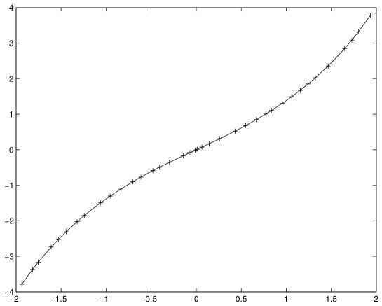
Figure 2: The prediction $\log\pi_{h}/(1-\pi_{h})$ as a function of $\log r$ together with the 40 measurements $\hat{\pi}_{h}(r_{i})$.

The second test is to obtain a solution of the differential equation (1) that describes the data. Let $f_{i},i=0,1,\dots,5$, be a basis of solutions for equation (1) defined by their behavior at $z=\frac{1}{2}$: $f_{i}^{(j)}(z=\frac{1}{2})=\delta_{ij}$. Since $f(z)=\frac{1}{2}-\pi_{h}(r(z))$ is odd with respect to $z=\frac{1}{2}$, it lies in the subspace of functions of the form $af_{1}+bf_{3}+cf_{5}$. We determine the constants $a,b$ and $c$ by requiring that $L=(\sum_{i}(\frac{1}{2}-\hat{\pi}_{h}(r_{i})-f(z(r_{i})))^{2})^{\frac{1}{2}}$ be minimum. The sum is over the 40 data. The three solutions $f_{1},f_{3}$ and $f_{5}$ were obtained numerically. Both Matlab and Mathematica give similar fits. These softwares have internal parameters controlling the required accuracy of the integration. These parameters can be pushed to a point where stronger requirement does not lead to any significant improvement on the minimum of $L$. Figure 2 has been drawn using the values $a,b$ and $c$ obtained for control parameters beyond this point. The largest among the differences $|\frac{1}{2}-\hat{\pi}_{h}(r_{i})-f(z(r_{i}))|,i=1,\dots,40$, is $3.6\times 10^{-4}$, smaller than the statistical error, and the standard deviation is $1.5\times 10^{-4}$. Similar results are obtained for $\pi_{v}$. The agreement is therefore excellent. As a comparison it is instructive to redo Cardy’s calculation testing his prediction for percolation. Since the publication of [1], better data were obtained for percolation by sites on a square lattice for $81$ rectangles with at least $10^{6}$ sites [7]. The samples contained over $10^{6}$ configurations. For these, the statistical errors are approximately $10^{-4}$ at the extremities of the interval ($r\in[0.142,7.067]$) and $10^{-3}$ in the middle. (At the extremities these data are therefore more precise than the present ones for the Ising model and at the center they are less precise.) The largest departure from duality is $4\times 10^{-4}$, almost exactly what is seen in Figure 1 for the present data. Comparing his prediction $\pi_{h}^{\text{perco}}(r(z))=3\Gamma(\frac{2}{3})z^{\frac{1}{3}}{}_{2}F_{1}(\frac{1}{3},\frac{2}{3},\frac{4}{3},z)/\Gamma(\frac{1}{3})^{2}$ with the data leads to $\max_{1\leq i\leq 81}|\pi_{h}^{\text{perco}}(r(z_{i}))-\hat{\pi}_{h}(r_{i})|=7.8\times 10^{-4}$ and to a standard deviation of $4.2\times 10^{-5}$. These results are similar to those just reported.

We mentioned earlier the possibility of describing the data with a hypergeometric function. The function

$$g(z)=\frac{6\Gamma(\frac{1}{3})}{\Gamma(\frac{1}{6})^{2}}z^{\frac{1}{6}}{}_{2}F_{1}({\textstyle{\frac{1}{6}}},{\textstyle{\frac{5}{6}}},{\textstyle{\frac{7}{6}}};z)$$

is odd around $z=\frac{1}{2}$, when shifted by $\frac{1}{2}$, and behaves as $z^{\frac{1}{6}}$ and $(1-z)^{\frac{1}{6}}$ when $z\rightarrow 0^{+}$ and $z\rightarrow 1^{-}$. Several data are now more than $2\times 10^{-3}$ apart from the corresponding values of $g$, a gap barely visible on a figure, but clearly out of any reasonable confidence interval. We may accept the solution of the differential equation as an analytic prediction for $\pi_{h}$ but we must reject the function $g(z)$.

Measurements were also made of the probability $\pi_{hv}$. As its behavior at $z=0$ and $z=1$ is also described by the exponent $\frac{1}{6}$, one may hope that the even subspace (around $z=\frac{1}{2}$) of the differential equation may contain a solution matching the data. This is not the case. The best fit in this subspace lies up to $6\times 10^{-3}$ away from the data, an unacceptable gap. (This disagreement has an advantage. It shows that the success of the fit for $\pi_{h}$ is not a consequence of the large freedom that a three-parameter fit gives.) Watts used the third singular vector to describe $\pi_{hv}$ for percolation. In the Verma module $V_{c=0,h=0}$, this vector is at level five, leading to a differential equation of order $5$. However the third one in $V_{c=\frac{1}{2},h=0}$ is at level 11 and the associated operator $P(z,\frac{d\ }{dz})$ is a polynomial of order $11$ in $\frac{d\ }{dz}$. It can be cast as

$$P(z,\frac{d\ }{dz})= \sum_{1\leq i\leq 11,\ i\text{\ odd}}((z(1-z))^{i-1}p_{i}(z(1-z))\frac{d^{i}\ }{dz^{i}}$$

$$+\sum_{2\leq i\leq 10,\ i\text{\ even}}(1-2z)((z(1-z))^{i-1}p_{i}(z(1-z))\frac{d^{i}\ }{dz^{i}}$$

with

$$p_{1}(u) =-{\textstyle{\frac{1}{81}}}\,u\left(-484-20465\,u+120702\,u^{2}+134456\,u^{3}+326536\,u^{4}\right)$$

$$p_{2}(u) =-{\textstyle{\frac{1}{81}}}\left(-484-65267\,u+555942\,{u}^{2}+2442422\,u^{3}+9038782\,{u}^{4}\right)$$

$$p_{3}(u) ={\textstyle{\frac{1}{162}}}\left(44318-1002950\,u-5132553\,u^{2}-12317152\,u^{3}+245463307\,u^{4}\right)$$

$$p_{4}(u) ={\textstyle{\frac{1}{486}}}\left(-412839-8111249\,u-42237350\,u^{2}+749236363\,u^{3}\right)$$

$$p_{5}(u) ={\textstyle{-{\frac{1}{1944}}}}\left(3492203+28198986\,u-1347384726\,{u}^{2}+5106251212\,u^{3}\right)$$

$$p_{6}(u) ={\textstyle{-{\frac{7}{1944}}}}\left(368339-27634444\,u+153070553\,u^{2}\right)$$

$$p_{7}(u) ={\textstyle{\frac{11}{1296}}}\left(554551-9066926\,u+29200567\,{u}^{2}\right)$$

$$p_{8}(u) ={\textstyle{\frac{11}{54}}}\left(-11842+75835\,u\right)$$

$$p_{9}(u) ={\textstyle{-{\frac{11}{18}}}}\left(-757+3457\,u\right)$$

$$p_{10}(u) ={\textstyle{-{\frac{110}{3}}}}$$

$$p_{11}(u) =1.$$

The differential equation $P(z,\frac{d\ }{dz})f(z)=0$ is again symmetric under any permutation of the three regular singular points $0,1$ and $\infty$. The exponents (with their degeneracies) are $0(2),\frac{1}{6}(2),\frac{1}{2}(1),1(1),\frac{5}{3}(2),\frac{5}{2}(1),\frac{14}{3}(1)$ and $6(1)$. The even subspace of the differential equation is of dimension 6 and the fit will therefore contain 6 parameters. Using the data of the last column of Table 3 and numerical integration of the differential equation, we obtain a best fit (in the same sense as the one used for $\pi_{h}$) that has a largest difference of $2.7\times 10^{-4}$ and a standard deviation of $1.3\times 10^{-4}$. These are excellent results well within the experimental windows. However we have tried to fit similarly the function $h(z)=\kappa z^{\frac{1}{6}}(1-z)^{\frac{1}{6}}$ with the constant $\kappa$ chosen such that $h(z=\frac{1}{2})=\hat{\pi}_{hv}(z=\frac{1}{2})$. While this function is not a solution, the 6-dimensional subspace of (numerical) even solutions contains a solution $\tilde{h}$ that approaches it extremely well (namely $\max_{z\in[0,1]}|\tilde{h}(z)-h(z)|\approx 10^{-6}$). Consequently the large dimension of the even subspace allows for functions that are not solution to be fitted within statistical errors and the fit for $\pi_{hv}$ is much less convincing than the one above for $\pi_{h}$ or than Watts’ prediction.

Acknowledments

It is a pleasure to thank R.P. Langlands, M.-A. Lewis and G. Watts for helpful discussions, A. Bourlioux for introducing us to the control of errors in integrating differential equations and H. Pinson and Ph. Zaugg for a careful reading of the manuscript.

E. L. gratefully acknowledges a fellowship from the NSERC Canada Scholarships Program and Y. S.-A. support from NSERC (Canada) and FCAR (Québec).

$r$	$V_{0}$	$H_{0}$	$\hat{\pi}_{h}$	$\hat{\pi}_{v}$	$\hat{\pi}_{hv}$
0.1443	4	24	0.02215	0.9779	0.02215
0.1624	6	32	0.03321	0.9668	0.03321
0.1732	6	30	0.04057	0.9594	0.04057
0.1999	6	26	0.06082	0.9392	0.06082
0.2165	6	24	0.07400	0.9257	0.07400
0.2362	6	22	0.09062	0.9093	0.09061
0.2665	8	26	0.1166	0.8830	0.1166
0.2887	6	18	0.1359	0.8647	0.1359
0.3248	6	16	0.1662	0.8341	0.1661
0.3464	8	20	0.1834	0.8164	0.1831
0.3849	8	18	0.2133	0.7865	0.2127
0.4330	8	16	0.2483	0.7518	0.2468
0.4949	8	14	0.2891	0.7111	0.2852
0.5413	10	16	0.3163	0.6833	0.3096
0.6186	10	14	0.3572	0.6429	0.3436
0.6662	10	13	0.3797	0.6202	0.3600
0.7423	12	14	0.4124	0.5878	0.3804
0.8660	10	10	0.4580	0.5421	0.3997
0.9326	14	13	0.4797	0.5203	0.4042
0.9897	16	14	0.4969	0.5028	0.4059
1.010	14	12	0.5029	0.4973	0.4058
1.066	16	13	0.5183	0.4812	0.4043
1.155	16	12	0.5419	0.4578	0.3996
1.299	12	8	0.5767	0.4232	0.3860
1.540	16	9	0.6277	0.3717	0.3544
1.732	16	8	0.6639	0.3364	0.3269
1.949	18	8	0.6999	0.3001	0.2952
2.165	20	8	0.7318	0.2679	0.2655
2.309	16	6	0.7516	0.2484	0.2469
2.598	18	6	0.7864	0.2135	0.2128
2.887	20	6	0.8163	0.1835	0.1833
3.175	22	6	0.8418	0.1580	0.1579
3.464	24	6	0.8643	0.1357	0.1357
3.753	26	6	0.8834	0.1166	0.1166
4.330	30	6	0.9137	0.08623	0.08623
4.619	32	6	0.9259	0.07416	0.07416
5.196	24	4	0.9452	0.05489	0.05489
5.629	26	4	0.9563	0.04370	0.04370
6.062	28	4	0.9651	0.03489	0.03489
6.928	32	4	0.9778	0.02218	0.02218

Table 3: The measurements $\hat{\pi}_{h}$, $\hat{\pi}_{v}$ and $\hat{\pi}_{hv}$.

List of captions

Table 1: $\hat{\pi}_{h}$ for three aspect ratios $r$ and five sizes.

Table 2: Estimates $\hat{\pi}_{h}$ using subsets of available data.

Table 3: The measurements $\hat{\pi}_{h}$, $\hat{\pi}_{v}$ and $\hat{\pi}_{hv}$.

Figure 1: Differences $\hat{\pi}_{h}(r_{a})-\hat{\pi}_{v}(r_{b})$ and $\hat{\pi}_{hv}(r_{a})-\hat{\pi}_{hv}(r_{b})$ for several pairs $(r_{a},r_{b}=r_{a}^{-1})$.

Figure 2: The prediction $\log\pi_{h}/(1-\pi_{h})$ as a function of $\log r$ together with the 40 measurements $\hat{\pi}_{h}(r_{i})$.

References

- [1] Cardy J L 1992 Critical percolation in finite geometries J. Phys. A 25 L201-L206
- [2] Cardy J L 1986 Effect of boundary conditions on the operator content of two-dimensional conformally invariant theories Nucl. Phys. B275 200–218
- [3] DiFrancesco P, Mathieu P and Sénéchal D 1996 Conformal Field Theory Springer Verlag
- [4] Dotsenko Vl S, Fateev V A 1984 Conformal algebra and multipoint correlation functions in 2D statistical models Nucl. Phys. 240 312–348
- [5] Langlands R P, Lewis M-A and Saint-Aubin Y 2000 Universality and conformal invariance for the Ising model in domains with boundary J. Stat. Phys. 98 131–244
- [6] Langlands R P, Pichet C, Pouliot P and Saint-Aubin Y 1992 On the universality of crossing probabilities in two-dimensional percolation J. Stat. Phys. 67 553–574
- [7] Langlands R P, Pouliot P and Saint-Aubin Y 1994 Conformal invariance in two-dimensional percolation Bull. AMS 30 1–61
- [8] Watts G M T 1996 A crossing probability for critical percolation in two dimensions J. Phys. A 29 L363-368