NTZ 10/2000

NRCPS-HE-2000-13

Abstract

The gonihedric model of random surfaces on a 3d Euclidean lattice has equivalent representation in terms of transfer matrix $K(Q_{i},Q_{f})$ which describes the propagation of loops $Q$. We extend the previous construction of loop transfer matrix to the case of nonzero self-intersection coupling constant $\kappa$. We introduce loop generalization of Fourier transformation which allows to diagonalize transfer matrices depending on symmetric difference of loops and express all eigenvalues of $3d$ loop transfer matrix through the correlation functions of the corresponding 2d statistical system. The loop Fourier transformation allows to carry out analogy with quantum mechanics of point particles, to introduce conjugate loop momentum P and to define loop quantum mechanics.

We also consider transfer matrix on $4d$ lattice which describes propagation of memebranes. This transfer matrix can also be diagonalized by using generalized Fourier transformation, and all its eigenvalues are equal to the correlation functions of the corresponding $3d$ statistical system. Particularly the free energy of the $4d$ membrane system is equal to the free energy of $3d$ gonihedric system of loops and is equal to the free energy of 2d Ising model.

1 Introduction

Various models of random surfaces built out of triangles embedded into continuous space $R^{d}$ and surfaces built out of plaquettes embedded into Euclidean lattice $Z^{d}$ have been considered in the literature [1, 2, 15]. These models are based on area action and suffer the problem of non-scaling behaviour of the string tension and the dominance of branched polymers [3]. Several studies have analyzed the physical effects produced by rigidity of the surface introduced by adding dimension-less extrinsic curvature term to the area action [4]

$$T\cdot S(area)+\frac{1}{\alpha}F(extrinsic~{}curvature),$$

where T is a string tension, $\alpha$ is dimension-less coupling constant and $F(ext~{}curv)\propto 1$ is dimension-less functional. Comprehensive review of work in this area up to 1997 can be found in [3].

In [5, 6] authors suggested so-called gonihedric model of random surfaces which is also based on the concept of extrinsic curvature, but it differs in two essential points from the models considered in the previous studies. First it claims that only extrinsic curvature term should be considered as the fundamental action of the theory

$$S=m\cdot A(extrinsic~{}curvature),$$

here $m$ has dimension of mass and there is no area term in the action. Secondly it is required that the dependence on the extrinsic curvature should be such that the action will have dimension of length $A(extrinsic~{}curvature)~{}~{}\propto~{}~{}length.$ This means that the action should measure the surfaces in terms of length and it should be proportional to the linear size of the surface, as it was for the path integral. The last property will guarantee that in the limit when the surface degenerates into a single world line the functional integral over surfaces will naturally transform into the Feynman path integral for point-like relativistic particle (see Figure 1,2)

$$m~{}A_{xy}(extrinsic~{}curvature)~{}~{}\rightarrow~{}~{}m\int^{y}_{x}dl.$$

As it was demonstrated in [6] quantum fluctuations generate the area term in the effective action

$$S_{eff}=m~{}A(extrinsic~{}curvature)~{}~{}+~{}~{}T_{eff}~{}S(area)~{}~{}+~{}~{}...,$$

that is nonzero string tension $T_{eff}$. Therefore at the tree level the theory describes free quarks with string tension equal to zero, but now quantum fluctuations generate nonzero string tension and, as a result, quark confinement [6]. The theory may consistently describe asymptotic freedom and confinement as it is expected to be the case in QCD.

Our aim is to find out what the continuum limit of this regularized theory of random surfaces is, and if indeed the continuum limit corresponds to nontrivial string theory, does it describe QCD phenomena. This is a complicated problem and one of the possible ways to handle the problem is to go further and to formulate the theory also on a lattice. An equivalent representation of the model on Euclidean lattice $Z^{d}$ has been formulated in [7]. This representation depends on dimension $d$ of the embedding space. In three dimensions it is a spin model in which the interaction between spins is organized in a very specific way (see equation (8) ).In high dimensions it is a gauge spin system which contains one, two and three plaquette interaction terms.

In this article I shall consider the above model of random surfaces embedded into 3d Euclidean lattice $Z^{3}$. The reason to focus on that particular case is motivated by the fact that one can geometrically construct the corresponding transfer matrix [12] and find its exact spectrum [13]. The spectrum of the transfer matrix which depends only on symmetric difference of initial and final loops has been evaluated exactly in terms of correlation functions of the 2d Ising model in [13]. This transfer matrix has the form [12]

$$K_{\kappa=0}(Q_{1},Q_{2})=exp\{-\beta~{}[k(Q_{1})+2l(Q_{1}\bigtriangleup Q_{2})+k(Q_{2})]~{}\},$$

where $Q_{1}$ and $Q_{2}$ are closed polygon-loops on a two-dimensional lattice, $k(Q)$ is the curvature and $l(Q)$ is the length of the polygon-loop $Q$ . This transfer matrix describes the propagation of the initial loop $Q_{1}$ to the final loop $Q_{2}$.

Figure 1: It is required that the action $A_{xy}$ should measure the surfaces in terms of length, as it was for the path integral. When a surface degenerates into a single world line we have natural transition to a path integral .

Our aim in this article is to extend these results in several directions. First to construct the transfer matrix for more general case of nonzero self-intersection coupling constant $\kappa$

$$K(Q_{1},Q_{2})~{}~{}=~{}~{}K_{\kappa=0}(Q_{1},Q_{2})~{}\cdot exp\{-4\kappa\beta~{}[k_{int}(Q_{1})+2l(Q_{1}\stackrel{{\scriptstyle\leftrightarrow}}{{\cap}}Q_{2})+k_{int}(Q_{2})]~{}\},$$

where $k_{int}(Q)$ is number of self-intersection vertices of the loop $Q$. For $\kappa=0$ this expression coincides with the previous one. In the limit $\kappa\rightarrow\infty,$ one can see that on every time slice there will be no loops with self-intersections and we have propagation of nonsingular self-avoiding oriented loops.

Secondly, I will demonstrate that diagonalization of any transfer matrices $K(Q_{1}\bigtriangleup Q_{2})$, which depend only on symmetric difference of loops $Q_{1}\bigtriangleup Q_{2}$ can be performed by using generalization of Fourier transformation in loop space. This transformation will be defined by using the loop eigenfunctions

$$\Psi_{P}(Q)=e^{i\pi s(P\cap Q)}$$

which are numbered by the loop momentum $P$ and $s(Q)$ is the area of the region with boundary loop $Q$. They are in a pure analogy with plane waves in quantum mechanics $\psi_{p}(x)=e^{ipx}$. We shall prove that any transfer matrix $K(Q_{1}\bigtriangleup Q_{2})$ can be diagonalized by using this loop Fourier transformation

$$K(P_{1},P_{2})=\sum_{\{Q_{1},Q_{2}\}}K(Q_{1}\bigtriangleup Q_{2})~{}e^{i\pi s(P_{1}\cap Q_{1})-i\pi s(P_{2}\cap Q_{2})}=\Lambda_{P_{1}}~{}\delta(P_{1},P_{2}),$$

here $\Lambda_{P}$ are eigenvalues depending on loop-momentum $P$. Because the transfer matrix plays the role of the evolution operator, one can define a corresponding Hamiltonian operator as $H(P)=-ln\Lambda(P).$ At this point one can talk about loop quantum mechanics which should be defined by using conjugate loop operators $\hat{Q}$ and $\hat{P}$ and the Hamiltonian $H(\hat{P},\hat{Q})$.

I shall also consider the model of random three-dimensional manifolds which are build by gluing together tetrahedra in continuous space $R^{4}$ and out of 3d cubes in 4d Euclidean lattice $Z^{4}$. This system has very close nature with the gonihedric model because in both cases the action is proportional to the linear size of the manifold [12]. In [12] the authors where able to construct a transfer matrix for this theory as well. This transfer matrix describes the propagation of two-dimensional membrane $M$ and our main result is that both theories can be solved exactly by using generalization of the Fourier transformation in loop and in membrane spaces. They represent two nontrivial theories in three and four dimensions respectively which can be solved exactly.

In the next sections I shall present background material, the definition of the system of random surfaces in continuous space as well as on Euclidean lattice and describe its basic properties. In the third section the construction of the transfer matrix for the loops will be extended to the case of nonzero self-intersection coupling constant $\kappa$. In the fourth main section we shall introduce the generalization of Fourier transformation in the loop space and demonstrate that loop Fourier transformation allows to diagonalize all transfer matrices which depend only on symmetric difference of loops. The net result is that all eigenvalues $\Lambda_{P}$ of 3d transfer matrix are exactly equal to the loop correlation functions of the corresponding 2d system

$$({\Lambda_{P_{\vec{r_{1}},...\vec{r_{n}}}}\over\Lambda_{\emptyset}})^{3d}~{}=~{}<\sigma_{\vec{r_{1}}}\cdot\cdot\cdot\sigma_{\vec{r_{n}}}>_{2d}.$$ (1)

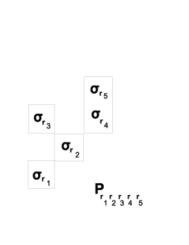
Figure 8: The loop momentum $P_{\vec{r_{1}},...\vec{r_{n}}}$ is defined by the vectors $\vec{r_{1}},...,\vec{r_{n}}$ and the corresponding eigenvalue $\Lambda_{P_{\vec{r_{1}},...\vec{r_{n}}}}$ is equal to the correlation function of the $n$ spins   $~{}~{}<\sigma_{\vec{r_{1}}}\cdot\cdot\cdot\sigma_{\vec{r_{n}}}>_{2d}$.

In this formula the loop momentum $P$ is defined by the vectors $\vec{r_{1}},...\vec{r_{n}}$ (see Figure 8). In its form the last relation is very close with the ones discussed in [16, 17, 18].

Figure 2: The random path and random surface with boundary points $X$ and $Y$. In both cases the action is proportional to the linear size of the geometrical fluctuation [6].

In the last section I shall consider the transfer matrix for membranes. This matrix also can be diagonalized by Fourier transformation and all its egenvalues are equal to the correlation functions of the corresponding 3d system. In particular we shall see that free energy of the membrane system is equal to the free energy of gonihedric system of loops and is equal to the free energy of 2d Ising model.

2 Random Surfaces and Path Integral

Surfaces in Continuous Space. Gonihedric string has been defined as a model of random surfaces with the action which is proportional to the linear size of the surface [5, 6]

$$m~{}\sum_{<ij>}\lambda_{ij}\cdot|\pi-\alpha_{ij}|^{\zeta}~{}~{}~{}~{}~{}~{}~{}~{}\zeta\leq(d-2)/d,$$ (2)

where $\lambda_{ij}$ is the length of the edge $<ij>$ of the triangulated surface $M$ and $\alpha_{ij}$ is the dihedral angle between two neighboring triangles of $M$ sharing a common edge $<ij>$ (see Figure 1,2) . The action was defined for the self-intersecting surfaces as well [6], it accounts self-intersections of different orders by ascribing weights to self-intersections. These weights are proportional to the length of the intersection multiplied by the angular factor which is equal to the sum of all angular factors corresponding to dihedral angles in the intersection [6] (see Figure 3)

$$\kappa~{}m~{}\sum_{<ij>}\lambda_{ij}\cdot(~{}|\pi-\alpha^{1}_{ij}|^{\zeta}+...+|\pi-\alpha^{r}_{ij}|^{\zeta}~{}).$$ (3)

The number of terms inside parentheses depends on the order of the intersection $r$, where $r$ is the number of triangles sharing the edge $<ij>$. Coupling constant $\kappa$ is called self-intersection coupling constant [6]. Thus the total action is equal to

$$A(M)=m~{}\sum_{<ij>}\lambda_{ij}\cdot|\pi-\alpha_{ij}|^{\zeta}~{}~{}+~{}m~{}\kappa~{}\sum_{<ij>}\lambda_{ij}\cdot(~{}|\pi-\alpha^{1}_{ij}|^{\zeta}+...+|\pi-\alpha^{r}_{ij}|^{\zeta}~{}).$$ (4)

Both terms in the action have the same dimension and the same geometrical nature, the action (2) measures two-dimensional surfaces in terms of length, self-intersections are also measured in terms of length (3). If $\kappa$ is small then self-intersections are permitted, if $\kappa$ increases then there is strong repulsion along the curves of self-intersections, and the surfaces tend to be self-avoiding [6].

The model is a natural extension of the Feynman path integral for point-like relativistic particle (see Figure 1,2). This can be seen from (2) in the limit when the surface degenerates into a single world line [6]

$$~{}~{}~{}~{}~{}~{}~{}~{}~{}~{}~{}~{}\sum_{<ij>}\lambda_{ij}\cdot|\pi-\alpha|^{\varsigma}~{}~{}\longleftrightarrow~{}~{}\sum_{<ij>}\lambda_{ij}.$$

Figure 3: The figure depicted the self-intersection of three planes and the associated action. In the given case $\alpha+\beta+\gamma=2\pi$.

At the classical level the string tension is equal to zero and quarks viewed as open ends of the surface are propagating freely without interaction $\sigma_{classical}=0$. This is because the action (2) is equal to the perimeter of the flat Wilson loop $A(M)\rightarrow m(R+T).$ As it was demonstrated in [6], quantum fluctuations generate nonzero string tension $\sigma_{quantum}=\frac{d}{a^{2}}~{}(1-ln\frac{d}{\beta}),$ where $d$ is the dimension of the spacetime, $\beta$ is the coupling constant, $a$ is a scaling parameter and $\varsigma=\frac{d-2}{d}$ in (2). In the scaling limit $\beta\rightarrow\beta_{c}=d/e$ the string tension has a finite limit.

We shall also consider similar model of random membranes with the action which is proportional to the linear size of the corresponding worldvolume. This action for three-dimensional manifold has been defined as

$$A(N)=m~{}\sum_{<i,j>}\lambda_{ij}\cdot|2\pi-\omega_{ij}|^{\zeta}$$ (5)

where $\lambda_{ij}$ is the length of the edge $<ij>$ of three-dimensional manifold $N$ which is constructed by gluing together three-dimensional tetrahedra through their triangular faces and $2\pi-\omega_{ij}$ is the deficit angle on the edge $<ij>$, here $\omega_{ij}$ is the sum of the dihedral angles between triangular faces of tetrahedra which have the common edge $<ij>$.

Equivalent spin system on a lattice [7]. In addition to the formulation of the theory in the continuum space the system allows an equivalent representation on Euclidean lattices where a surface is associated with a collection of plaquettes [7]. The corresponding statistical weights are proportional to the total number of non-flat edges $n_{2}(M)$ of the surface $M$ as it is defined in (2) [7]. The edges are non-flat when the dihedral angle between plaquettes is equal to $\pi/2$. The surfaces may have self-intersections in the form of four plaquettes intersecting on a link. The weight associated with self-intersections is proportional to $4\kappa n_{4}$ where $n_{4}(M)$ is the number of edges with four intersecting plaquettes, and $\kappa$ is the self-intersection coupling constant (3) . The edges of the surface with self-intersections comprise the singular part of the surface. The edges of the surface where only two plaquettes are intersecting comprise the regular part of the surface.

The partition function can be represented as a sum over two-dimensional surfaces $M$ of the type described above, embedded into a three-dimensional lattice:

$$Z(\beta)=\sum_{\{surfaces~{}M\}}e^{-2\beta~{}A(M)},$$ (6)

where $A(M)$ is the energy of the surface $M$ constructed from plaquettes

$$A_{gonihedric}(M)=n_{2}(M)+4\kappa n_{4}(M).$$ (7)

To study statistical and scaling properties of the system one can directly simulate surfaces by gluing together plaquettes following the rules described above, or to use the duality between random surfaces and spin systems on Euclidean lattice. This duality allows to study equivalent spin system with specially adjusted interaction between spins [7]. In three dimensions the corresponding Hamiltonian is equal to [7]

$$H_{gonihedric}^{3d}=-2\kappa\sum_{\vec{r},\vec{\alpha}}\sigma_{\vec{r}}\sigma_{\vec{r}+\vec{\alpha}}+\frac{\kappa}{2}\sum_{\vec{r},\vec{\alpha},\vec{\beta}}\sigma_{\vec{r}}\sigma_{\vec{r}+\vec{\alpha}+\vec{\beta}}-\frac{1-\kappa}{2}\sum_{\vec{r},\vec{\alpha},\vec{\beta}}\sigma_{\vec{r}}\sigma_{\vec{r}+\vec{\alpha}}\sigma_{\vec{r}+\vec{\alpha}+\vec{\beta}}\sigma_{\vec{r}+\vec{\beta}},$$ (8)

where $\vec{r}$ is a three-dimensional vector on the lattice $Z^{3}$, the components of which are integer and $\vec{\alpha}$, $\vec{\beta}$ are unit vectors parallel to the axes. The interface energy of this lattice spin system coincides with the linear action (4), (7).

The form of the Hamiltonian $H(\kappa)$ and the symmetry of the system essentially depend on $\kappa$: when $\kappa\neq 0$ one can flip the spins on arbitrary parallel layers and thus the degeneracy of the ground state is equal to $3\cdot 2^{N}$, where $N^{3}$ is the size of the lattice. When $\kappa=0$ the system has even higher symmetry, all states, including the ground state are exponentially degenerate. This degeneracy of the ground state is equal to $2^{3N}$ [12]. This is because now one can flip the spins on arbitrary layers, even on intersecting ones. The corresponding Hamiltonian contains only exotic four-spin interaction term.

The understanding of critical behaviour of this system comes from the analysis of the transfer matrix [12] which describes the propagation of the closed loops $Q$ in time direction with an amplitude which is proportional to the sum of the length $l(Q)$ of the loop and of its total curvature $k(Q)$. Because the amplitude essentially depends on length, as it takes place in 2d Ising model, this result directs to the idea that the system in 3d will show the phase transition which should be of the same nature as it is in 2d Ising system and that the transfer matrix describes the propagation of an almost free string of Ising model [12]. Direct numerical Monte-Carlo simulations [19] and analytical solution of different approximations to the full transfer matrix confirm strong connection with the 2d Ising model [13].

Below I shall remind the derivation of the corresponding transfer matrix for the case $\kappa=0$, which is based on geometrical theorem proven in [11] and then I shall derive the transfer matrix for more general case $\kappa\neq 0$. This will allow to study physical picture of string propagation which follows from the transfer matrix approach.

3 Loop Transfer Matrix

Geometrical Theorem [11]. In this section I shall review the construction of the transfer matrix for the system (8) with $\kappa=0$ [12]

$$H_{gonihedric}^{3d}(\kappa=0)=-\frac{1}{2}\sum_{\vec{r},\vec{\alpha},\vec{\beta}}\sigma_{\vec{r}}\sigma_{\vec{r}+\vec{\alpha}}\sigma_{\vec{r}+\vec{\alpha}+\vec{\beta}}\sigma_{\vec{r}+\vec{\beta}},$$ (9)

and then extend the result to nonzero case $\kappa\neq 0$.

In order to find transfer matrix for this system we have to use geometrical theorem proven in [11]. The geometrical theorem provides an equivalent representation of the action $A(M)$ in terms of total curvature $k(E)$ of the polygons which appear in the intersection of the two-dimensional plane $E$ with the given two-dimensional surface $M$ (see Figure 4,5). This curvature $k(E)$ should then be integrated over all planes $E$ intersecting the surface $M$.

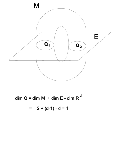
Figure 4: The geometrical theorem provides an equivalent representation of the action $A(M)$ in terms of total curvature $k(E)$ of the curves $Q_{1}(E),...,Q_{k}(E)$ which appear in the intersection of the (d-1)-dimensional plane $E$ with the given two-dimensional surface $M$. The curvature $k(E)$ should then be integrated over all planes $E$ intersecting the surface $M$.

The intersection of the two-dimensional plane $E$ with the polyhedral surface $M$ is the union of the polygons (see Figure 5)

$$Q_{1}(E),...,Q_{k}(E)$$

and the absolute total curvature $k(E)$ of these polygons is equal to

$$k(E)=\sum^{k}_{i=1}k(Q_{i})=\sum_{<i,j>}|\pi-\alpha^{E}_{ij}|,$$ (10)

where $\alpha^{E}_{ij}$ are the angles of these polygons. They are defined as the angles in the intersection of the two-dimensional plane $E$ with the edge $<ij>$ [11] (see Figure 5). The meaning of (10) is that it measures the total revolution of the tangent vectors to polygons $Q_{1}(E),...,Q_{k}(E)$. Integrating the total curvature $k(E)$ (10) over all intersecting planes $E$ we shall get the action $A(M)$ [11]

$$A(M)=\frac{1}{2\pi}\int_{\{E\}}k(E)dE.$$ (11)

Figure 5: Intersection of the polyhedral surface $M$ by the plane $E$. The image of the surface on the plane is a polygon $P$ and its curvature is equal to $k(E)$.

Geometrical Theorem on a lattice [12]. One can find the same representation (11) for the action $A(M)$ on a cubic lattice $Z^{3}$ introducing a set of planes $\{E_{x}\},\{E_{y}\},\{E_{z}\}$ perpendicular to $x,y,z$ axis on the dual lattice $Z^{3}_{d}$. These planes will intersect a given surface $M$ and on each of these planes we shall have an image of the surface $M$. Every such image is represented as a collection of closed polygons $Q(E)$ appearing in the intersection of the plane with surface $M$ (see Figure 6). The energy of the surface $M$ is equal now to the sum of the total curvature $k(E)$ of all these polygons on different planes

$$A(M)=\sum_{\{E_{x},E_{y},E_{z}\}}k(E).$$ (12)

The total curvature $k(E)$ is simply the total number of polygon right angles. In the case when the self-intersection coupling constant $\kappa=0$ is equal to zero we must compute the total curvature $k(E)$ of these polygons ignoring angles at the self-intersection points!

With (12) the partition function of the system can be written in the form

$$Z(\beta)=\sum_{\{M\}}exp\{-2\beta\sum_{\{E\}}k(E)\}$$ (13)

where the sum in the exponent can be represented as a product

$$exp\{-2\beta\sum_{\{E\}}k(E)\}=\prod_{\{E\}}e^{-2\beta k(E)}=\prod_{\{E_{z}\}}e^{-2\beta k(E_{z})}\prod_{\{E_{y}\}}e^{-2\beta k(E_{y})}\prod_{\{E_{x}\}}e^{-2\beta k(E_{x})}.$$ (14)

The goal is to express the energy functional (12) and the product (14) in terms of quantities defined only on two-dimensional planes in one fixed direction, let’s say through $\{E_{z}\}$.

Transfer Matrix for $\kappa=0$ [12]. The question is: what kind of information do we need to know on these planes $\{E_{z}\}$ to recover the values of the total curvature $k(E_{x})$ and $k(E_{y})$ on the planes $\{E_{y}\}$ and $\{E_{x}\}$ for the given surface $M$?

Let us consider the sequence of two planes $E_{z}^{i}$ and $E_{z}^{i+1}$ and denote by $Q_{i}$ the polygon-image of the surface $M$ on the plane $E_{z}^{i}$ and by $Q_{i+1}$ the polygon-image of $M$ on the plane $E_{z}^{i+1}$. The contribution to the curvature $k(E_{x})+k(E_{y})$ of the polygons which are on the perpendicular planes between $E^{i}_{z}$ and $E^{i+1}_{z}$ is equal to the length of the polygons $Q_{i}$ and $Q_{i+1}$ without length of the common bonds [12]

$$l(Q_{i})+l(Q_{i+1})-2\cdot l(Q_{i}\cap Q_{i+1})=l(Q_{i}\bigtriangleup Q_{i+1}),$$ (15)

where the polygon-loop  $Q_{1}\bigtriangleup Q_{2}~{}\equiv~{}Q_{1}\cup Q_{2}~{}\backslash~{}Q_{1}\cap Q_{2}$  is a union of links $Q_{1}\cup Q_{2}$ without common links $Q_{1}\cap Q_{2}$. Therefore (see formula (12))

$$A(M)=\sum_{\{E\}}k(E)=\sum_{\{E_{z}\}}k(Q_{i})+l(Q_{i}\bigtriangleup Q_{i+1}).$$ (16)

The partition function (13) can be now represented in the form

$$Z(\beta)=\sum_{\{Q_{1},Q_{2},...,Q_{N}\}}~{}K_{\beta}(Q_{1},Q_{2})\cdots K_{\beta}(Q_{N},Q_{1})=trK^{N}_{\beta},$$ (17)

where $K_{\beta}(Q_{1},Q_{2})$ is the transfer matrix of size $\gamma\times\gamma$, defined as

$$K^{gonihedric}_{\kappa=0}(Q_{1},Q_{2})=exp\{-\beta~{}[k(Q_{1})+2l(Q_{1}\bigtriangleup Q_{2})+k(Q_{2})]~{}\},$$ (18)

where $Q_{1}$ and $Q_{2}$ are closed polygon-loops on a two-dimensional lattice $T^{2}$ of size $N\times N$ and $\gamma=2^{N^{2}}$ is the total number of polygon-loops on a lattice $T^{2}$. The transfer matrix (18) can be viewed as describing the propagation of the polygon-loop $Q_{1}$ at time $\tau$ to another polygon-loop $Q_{2}$ at the time $\tau+1$ (see Figure 7).

Figure 6: The set of planes $\{E_{x}\},\{E_{y}\},\{E_{z}\}$ perpendicular to $x,y,z$ axis intersect a given surface $M$ in the middle of the links. On each of these planes we shall have an image of the surface $M$. Every such image is represented by closed polygon-loops $P(E)$ appearing in the intersection of the plane with surface $M$. The energy of the surface $M$ is equal to the sum of the total curvature $k(E)$ on all these planes as it is given by the formula (12). For the surface on the picture this sum is equal to $A=16+20+20=56$ times $a{\pi\over 2}$.

Figure 7: The transfer martix (18) can be viewed as describing the propagation of the polygon-loop $P_{1}$ at time $\tau$ to another polygon-loop $P_{2}$ at the time $\tau+1$. For the surface on the picture we have $k(P_{1})=4,k(P_{2})=12,l(\emptyset\bigtriangleup P_{1})=12,l(P_{1}\bigtriangleup P_{2})=16,l(P_{2}\bigtriangleup\emptyset)=12$. Summing all these quantities in accordance with the formula (16) we shall get $A(M)=4+12+12+16+12=56$ times $a{\pi\over 2}$. This, as it should, coincides with the previous result.

The functional $k(Q)$ is the total curvature of the polygon-loop $Q$ which is equal to the number of corners of the polygon ( the vertices with self-intersection are not counted!) and $l(Q)$ is the length of $Q$ which is equal to the number of its links. The length functional $l(Q_{1}\bigtriangleup Q_{2})$ was defined above (15) . The operation $\bigtriangleup$ maps two polygon-loops $Q_{1}$ and $Q_{2}$ into a polygon-loop $Q=Q_{1}\bigtriangleup Q_{2}$ . The length functional $l(Q_{1}\bigtriangleup Q_{2})$ defines a distance between two polygon-loops $Q_{1}$ and $Q_{2}$.

The eigenvalues of the transfer matrix $K_{\beta}(Q_{1},Q_{2})$ define all statistical properties of the system and can be found as a solution of the following integral equation in the loop space $\Pi$ [13]

$$\sum_{\{Q_{2}\}}K_{\beta}(Q_{1},Q_{2})~{}\Psi(Q_{2})=\Lambda(\beta)~{}\Psi(Q_{1}),$$ (19)

where $\Psi(Q)$ is a function on loop space. The Hilbert space of complex functions $\Psi(Q)$ on $\Pi$ will be denoted as $H=L^{2}(\Pi)$. The eigenvalues define the partition function (13)

$$Z^{3d}(\beta)=\Lambda^{N}_{0}+...+\Lambda^{N}_{\gamma-1},$$ (20)

and in the thermodynamical limit the free energy is equal to

$$-\beta~{}f_{3d}(\beta)=\lim_{N\rightarrow\infty}\frac{1}{N^{3}}~{}ln~{}Z^{3d}(\beta)=\lim_{N\rightarrow\infty}\frac{1}{N^{2}}~{}ln~{}\Lambda_{0}.$$ (21)

Finite time propagation amplitude of an initial loop $Q_{i}$ to a final loop $Q_{f}$ for the time interval $t=M/\beta$ can be defined as

$$K(Q_{i},Q_{f})=\Lambda^{-M}_{0}\sum_{\{Q_{1},Q_{2},...,Q_{M-1}\}}~{}K_{\beta}(Q_{i},Q_{1})\cdots K_{\beta}(Q_{M-1},Q_{f}),$$ (22)

where we have introduced natural normalization to the biggest eigenvalue $\Lambda_{0}$ and $M\leq N$.

Loop Transfer Matrix for $\kappa\neq 0$. We would like to generalize the construction of the transfer matrix to the case of nonzero self-intersection coupling constant $\kappa$. As we already mentioned above surfaces on a lattice may have self-intersections and we associate the coupling constant $\kappa$ with these self-intersection edges of the surface. When we consider the sections of the lattice surface $M$ by the planes $E$ the self-intersection edges will appear on a plane as polygon-loops with self-intersections. When $\kappa=0$ we have been instructed to compute the total curvature $k(E)$ of these polygon-loops simply ignoring angles at the self-intersection points. Now when $\kappa\neq 0$ we have to take into account self-intersection vertices of polygon-loops.

The contribution to the action which comes from simple polygon right angles is the same as before (16)

$$\sum_{\{E_{z}\}}k(Q_{i})+l(Q_{i}\bigtriangleup Q_{i+1}).$$ (23)

The contribution coming from self-intersections should be divided into contribution coming from vertical and horizontal edges of the surface. The vertical and horizontal edges of the surface are defined relative to the ”time” planes $E_{z}$. The contribution from vertical edges is simply the number of self-intersection vertices of loops on $E_{z}$ planes

$$4\kappa\cdot\sum_{\{E_{z}\}}k_{int}(Q_{i}),$$ (24)

where $k_{int}(Q)$ is the number of self-intersection vertices of loop $Q$.

To count contribution from horizontal edges of the surface one should introduce the orientation of the polygon-loops on every $E_{z}$ plane. The same orientation is ascribed to all polygon-loops on a given plane $E_{z}$: clock-wise or anti-clock-wise. Orientation is automatic if $Q$ is thought as interface between spins. Conjugation $\stackrel{{\scriptstyle\rightarrow}}{{Q}}$ $\rightarrow$ $\stackrel{{\scriptstyle\leftarrow}}{{Q}}$ is equivalent to $Z_{2}$ spin flip. So there is $\stackrel{{\scriptstyle\rightarrow}}{{Q}}$ and $\stackrel{{\scriptstyle\leftarrow}}{{Q}}$ with opposite orientation.

Now let us consider oriented polygon-loops on two planes $E^{i}_{z}$ and $E^{i+1}_{z}$. Then one should select that bonds on these polygon-loops which are common. Only bonds with the opposite orientation should be counted. The number of common bonds with opposite orientation we shall denote as $l(Q_{i}\stackrel{{\scriptstyle\leftrightarrow}}{{\cap}}Q_{j})$. The notation $\cap$ is used to denote the common bonds, the symbol $\leftrightarrow$ on the top of it to denote that they should have opposite orientations. Therefore the contribution from horizontal edges can be expressed as

$$4\kappa\cdot\sum_{\{E_{z}\}}l(Q_{i}\stackrel{{\scriptstyle\leftrightarrow}}{{\cap}}Q_{j})$$ (25)

and the contribution from all self-intersections as

$$4\kappa\cdot\sum_{\{E_{z}\}}~{}k_{int}(Q_{i})+l(Q_{i}\stackrel{{\scriptstyle\leftrightarrow}}{{\cap}}Q_{i+1}).$$ (26)

The total action (7) now takes the form:

$$A(M)=\sum_{\{E_{z}\}}~{}k(Q_{i})+l(Q_{i}\bigtriangleup Q_{i+1})+4\kappa\cdot[~{}k_{int}(Q_{i})+l(Q_{i}\stackrel{{\scriptstyle\leftrightarrow}}{{\cap}}Q_{i+1})~{}].$$ (27)

The partition function (13) can be now represented in the same form (17) where $K_{\beta}(Q_{1},Q_{2})$ is again the transfer matrix of size $\gamma\times\gamma$, defined as

$$K_{\beta}(Q_{1},Q_{2})~{}~{}~{}~{}=~{}~{}~{}~{}exp\{-\beta~{}[k(Q_{1})+2l(Q_{1}\bigtriangleup Q_{2})+k(Q_{2})]\}\cdot~{}~{}~{}~{}~{}~{}~{}~{}~{}~{}$$

$$exp\{-4\kappa\beta~{}[k_{int}(Q_{1})+2l(Q_{1}\stackrel{{\scriptstyle\leftrightarrow}}{{\cap}}Q_{2})+k_{int}(Q_{2})]\},$$ (28)

where $Q_{1}$ and $Q_{2}$ are closed oriented polygon loops on a two-dimensional lattice $T^{2}$ of size $N\times N$ and $\gamma$ is the total number of polygon-loops on a lattice $T^{2}$. Let us now consider the limit

$$\kappa\rightarrow\infty,$$

then from our expression for the transfer matrix (28) one can conclude that on every time slice there will be no polygon-loops with self-intersections. This means that they are just nonsingular self-avoiding oriented loops. In addition there is strong correlation between loops on consecutive planes: common bonds with opposite orientation are also strongly suppressed. Which means that propagation of oriented loop in time has small probability to invert its orientation.

4 Loop Fourier transformation

In the approximation when we drop the curvature term in the expression (18) for the loop transfer matrix $K(Q_{1},Q_{2})$ the spectrum of the matrix has been evaluated exactly in the articles [13, 12]. In this section I shall present an alternative method of derivation which is based on generalization of Fourier transformation and allows to carry out analogy with quantum mechanics of point particles and to emphasize generality of the approach.

I shall consider two different approximations to the initial transfer matrix (18) suggested in [12] and [13]. In the first one it was suggested to substruct the term $2k(Q_{1}\cup Q_{2})$ and to consider the transfer matrix of the form [12]

$$\tilde{K}(Q_{1}\bigtriangleup Q_{2})=exp\{-\beta~{}[k(Q_{1}\bigtriangleup Q_{2})+2l(Q_{1}\bigtriangleup Q_{2})]~{}\},$$ (29)

and in the second one to consider the transfer matrix [13]

$$K(Q_{1}\bigtriangleup Q_{2})=exp\{-2\beta~{}l(Q_{1}\bigtriangleup Q_{2})~{}\}.$$ (30)

In both cases the transfer matrix depends only on the symmetric difference $Q_{1}\bigtriangleup Q_{2}$ and the integral equation (19) take the form

$$\sum_{\{Q_{2}\}}K_{\beta}(Q_{1}\bigtriangleup Q_{2})~{}\Psi(Q_{2})=\Lambda(\beta)~{}\Psi(Q_{1}).$$ (31)

The fact that transfer matrix now depends only on the symmetric difference is of paramount importance in solving these models. The reason is that we can make a change of variable, from $Q_{2}$ to $Q$ at fixed $Q_{1}$ [13]

$$Q=Q_{1}\bigtriangleup Q_{2}$$ (32)

and see that equation transforms to the form

$$\sum_{\{Q\}}K_{\beta}(Q)~{}\Psi(Q\bigtriangleup Q_{1})=\Lambda(\beta)~{}\Psi(Q_{1}).$$ (33)

The integral equation will be solved if we can find the set of loop functions $\Psi(Q)$ which satisfy the following functional equation on loop space $\Pi$

$$\Psi(Q\bigtriangleup Q_{1})=\Psi(Q)\cdot\Psi(Q_{1}).$$ (34)

For these functions the equation (33) reduces to

$$\sum_{\{Q\}}K_{\beta}(Q)~{}\Psi(Q)=\Lambda(\beta)$$ (35)

and we can find all eigenvalues. The constant function $\Psi=1$ is the solution of the functional equation (34) and due to Frobenius-Perron theorem corresponds to the largest and non-degenerate eigenvalue $\Lambda_{\emptyset}$ of the symmetric transfer matrix $K(Q_{1}\bigtriangleup Q_{2})$.

The functional equation (34) is analogous to the equation $\psi(x+y)=\psi(x)\cdot\psi(y)$ appearing in ordinary quantum mechanics, which allows to find all eigenvectors and eigenvalues of the integral equation

$$\int K_{\beta}(x-y)\psi(y)dx=\lambda(\beta)\psi(y),~{}~{}~{}~{}~{}~{}~{}~{}K_{\beta}(x-y)=exp(-\beta(x-y)^{2})$$ (36)

with the well known solutions

$$\psi(x)=e^{ipx},~{}~{}~{}~{}~{}~{}~{}~{}~{}~{}~{}~{}\lambda_{p}(x)=e^{-p^{2}/4\beta}.$$

Our idea is to find all solutions of the functional equation (34) and the analog of the plane wave solution in loop space. From functional equation (34) it follows that if $Q=Q_{1}$ then

$$\Psi(\emptyset)=\Psi^{2}(Q)$$ (37)

and if $Q=\emptyset$ then $\Psi(\emptyset)$ is equal to zero or to one, therefore nontrivial solution is

$$\Psi^{2}(Q)=1~{}~{}~{}~{}~{}\Rightarrow~{}~{}~{}~{}~{}\Psi(Q)=\pm 1.$$ (38)

This suggests the following form of the eigenfunctions

$$\Psi_{P}(Q)=e^{i\pi s(P\cap Q)}$$ (39)

which are numbered by the loop momentum $P$ and take values $\pm 1$. The $s(Q)$ is the area of the region with the boundary loop $Q$. These solutions are in pure analogy with plane waves in quantum mechanics . To check that they are indeed solutions of the functional equation (34) we have to use the set identity

$$(Q_{1}\bigtriangleup Q_{2})\cap P=(Q_{1}\cap P)\bigtriangleup(Q_{2}\cap P)$$ (40)

which is easy to verify and the relation $s(Q_{i})+s(Q_{i+1})-2\cdot s(Q_{i}\cap Q_{i+1})=s(Q_{i}\bigtriangleup Q_{i+1})$. To carry out the analogy with plane wave solution of quantum mechanics deeper one should interpret the loop $P$ as a loop momentum conjugate to a loop coordinate variable $Q$. To prove orthogonality of these loop wave functions let us compute the product

$$\Psi_{P_{1}}\cdot\Psi_{P_{2}}=\sum_{\{Q\}}\Psi_{P_{1}}(Q)~{}\Psi_{P_{2}}(Q)=\sum_{\{Q\}}e^{i\pi s(P_{1}\cap Q)+i\pi s(P_{2}\cap Q)}=\sum_{\{Q\}}e^{i\pi s((P_{1}\bigtriangleup P_{2})\cap Q)}$$ (41)

where we again used the above set identity and the relation (15) for $s(Q)$. The last sum is equal to zero if $P_{1}\bigtriangleup P_{2}\neq\emptyset$ and is equal to the number of loops $\gamma$ on the lattice if $P_{1}\bigtriangleup P_{2}=\emptyset$, thus

$$\sum_{\{Q\}}e^{i\pi s((P_{1}\bigtriangleup P_{2})\cap Q)}=2^{N^{2}}\delta(P_{1},P_{2}).$$ (42)

The last statement follows from the fact that the product between the constant function $\Psi_{\emptyset}=1$, corresponding to the largest and non-degenerate eigenvalue $\Lambda_{\emptyset}$, and all others $exp(i\pi s(P\cap Q))$ is equal to zero if $P$ is nonempty

$$\sum_{\{Q\}}1\cdot e^{i\pi s((P\cap Q)}=0,~{}~{}~{}~{}if~{}~{}~{}~{}~{}P\neq\emptyset.$$ (43)

The number of functions in this orthogonal set is equal therefore to the number of closed loops $P$, that is $\gamma=2^{N^{2}}$.

Having in hand all eigenfuctions we can find all eigenvalues from (35) for transfer matrices (29) and (30)

$$\tilde{\Lambda}_{P}=\sum_{\{Q\}}e^{-i\pi s(P\cap Q)-\beta[k(Q)+2l(Q)]}~{}~{}~{}~{}~{}~{}~{}~{}~{}~{}\Lambda_{P}=\sum_{\{Q\}}e^{-i\pi s(P\cap Q)-2\beta l(Q)}.$$ (44)

Because the expression $\sum_{\{Q\}}e^{-2\beta l(Q)}$ is the partition function of the 2d Ising model [8, 9] and $\sum_{\{Q\}}e^{-\beta[2l(Q)+k(Q)]}$ is the partition function $\tilde{Z}^{2d}$ of the two-dimensional model solved in [12] we see that the largest eigenvalue $\Lambda_{\emptyset}$ is exactly equal to a corresponding partition function

$$\tilde{\Lambda}_{\emptyset}=\tilde{Z}^{2d}~{}~{}~{}~{}~{}~{}~{}~{}~{}~{}\Lambda_{\emptyset}=Z^{2d-Ising}.$$ (45)

For the ratio of eigenvalues we shall have

$${\Lambda_{P}\over\Lambda_{\emptyset}}~{}=~{}\sum_{\{Q\}}e^{-i\pi s(P\cap Q)-2\beta l(Q)}/Z^{2d-Ising}~{}\equiv~{}<e^{-i\pi s(P\cap Q)}>_{Q}$$ (46)

which is identically equal to the spin correlation functions of the 2d Ising model

$${\Lambda_{P_{\vec{r_{1}},...\vec{r_{n}}}}\over\Lambda_{\emptyset}}~{}=~{}<\sigma_{\vec{r_{1}}}\cdot\cdot\cdot\sigma_{\vec{r_{n}}}>_{2dIsing}.$$ (47)

In this formula the loop momentum $P$ is defined by the vectors $\vec{r_{1}},...\vec{r_{n}}$. In particular for the smallest (one-box) loop momentum $P=\Box$ we shall have

$${\Lambda_{\Box}\over\Lambda_{\emptyset}}~{}=~{}<\sigma_{\vec{r}}>~{}=~{}\mu(\beta)$$ (48)

which coincides with the magnetization of 2d Ising model. Because it does not depend on position of the loop on the lattice, this eigenvalue is $N^{2}$ degenerate. For the two-box loop momentum $P=~{}\sqsubset\sqsupset$ consisting of two neighboring boxes we shall have

$${\Lambda_{\sqsubset\sqsupset}\over\Lambda_{\emptyset}}~{}=~{}<\sigma_{\vec{r}}\sigma_{\vec{r+1}}>~{}=~{}-u(\beta)$$ (49)

which is $2N^{2}$ degenerate and after summation over all $2N^{2}$ bonds of the lattice we shall get the internal energy of the 2d Ising model.

We can also use loop wave functions to define generalized loop-Fourier transformation as

$$\Psi(P)={1\over 2^{N^{2}}}\sum_{\{Q\}}e^{i\pi s(P\cap Q)}\Psi(Q)$$ (50)

and then compute the loop Fourier transformation of the transfer matrices (29) and (30) as:

$$K(P_{1},P_{2})=\sum_{\{Q_{1},Q_{2}\}}K(Q_{1}\bigtriangleup Q_{2})e^{i\pi s(P_{1}\cap Q_{1})-i\pi s(P_{2}\cap Q_{2})}=\Lambda_{P_{1}}\sum_{\{Q_{2}\}}e^{i\pi s(P_{1}\cap Q_{2})-i\pi s(P_{2}\cap Q_{2})}$$

$$=\Lambda_{P_{1}}\delta(P_{1},P_{2}).~{}~{}~{}~{}~{}~{}~{}~{}~{}~{}~{}~{}~{}~{}~{}~{}~{}~{}~{}~{}~{}~{}~{}~{}~{}~{}~{}~{}~{}~{}~{}~{}~{}~{}~{}~{}~{}~{}~{}~{}~{}~{}~{}~{}~{}~{}$$ (51)

The finite time propagation amplitude of an initial loop $P_{i}$ to the final loop $P_{f}$ for the time interval $t=M/\beta$ (22) we have

$$K(P_{i},P_{f})=({\Lambda_{P_{i}}\over\Lambda_{\emptyset}})^{M}~{}~{}\delta(P_{i},P_{f})=e^{Mln({\Lambda_{P_{i}}\over\Lambda_{\emptyset}})}~{}~{}\delta(P_{i},P_{f})=e^{-MH(P_{i})}~{}~{}\delta(P_{i},P_{f}),$$ (52)

therefore for the loop Hamiltonian we shall get

$$H(P)=-ln({\Lambda_{P}\over\Lambda_{\emptyset}})$$ (53)

where $H(P)$ is the energy of the coherent state with loop momentum $P$.

Spin system which corresponds to the matrix $K(Q_{i}\bigtriangleup Q_{i+1})$ (30). The natural question which arises here is how nontrivial is the 3d system which has been solved in this way? To make the answer as clear as possible we should go back and express the system which has been solved again in terms of spins on a 3d lattice and to see what is left out of original interactions.

We ignore the curvature terms $k(Q_{i})$ in the transfer matrix, this means that we ignore the contribution coming from the edges of the surface which are along the time direction, or $z$ direction. The contribution coming from the edges which are parallel to the $x$ and $y$ direction are left and their contribution is equal to (15)

$$\sum_{\{E_{z}\}}l(Q_{i}\bigtriangleup Q_{i+1}).$$ (54)

In terms of spin variables the original action can be expressed as a sum of energies coming from all edges of the surface (see formulas (5a) and (7) in [7])

$$H=\sum_{over~{}all~{}edges}H_{edge},$$ (55)

where

$$H_{edge}=U_{1}U_{-1}+U_{1}U_{-1}=\sigma_{1}\sigma_{2}\sigma_{-1}\sigma_{-2}.$$ (56)

is a four-spin interaction term with spins distributed around the edge. Because we ignore the edges in the $z$ direction, we have to sum in (55) only over $A_{edges}$ in $x$ and $y$ direction. This corresponds to the summation over four-spin interaction terms (56) which lie only on the planes $E_{x}$ and $E_{y}$. These planes are normal to the $x$ and $y$ direction. Therefore our approximation corresponds to the 3d lattice spin system in which four-spin interactions take place only on vertical planes $E_{x}$ and $E_{y}$

$$H_{Q_{1}\bigtriangleup Q_{2}}=\sum_{E_{x},E_{y}}\sigma\sigma\sigma\sigma.$$ (57)

It is obvious that this spin system can not be factored into non interacting two-dimensional subsystems. We can ask what is the effective interaction between spins which lie on a given two-dimensional $E_{z}$ plane? Let us label spins which are on that plane as $\sigma$, spins which are on the previous plane as $\lambda$, and spins which are on the next plane as $\mu$. The part of the Hamiltonian which contains only $\sigma$ spins can be written in the form:

$$\sum_{i}\sigma_{i}\sigma_{i+1}\lambda_{i}\lambda_{i+1}+\sigma_{i}\sigma_{i+1}\mu_{i}\mu_{i+1}=\sum_{i}(\lambda_{i}\lambda_{i+1}+\mu_{i}\mu_{i+1})\sigma_{i}\sigma_{i+1}=\sum_{i}J_{eff}\sigma_{i}\sigma_{i+1},$$ (58)

where the effective coupling $J_{eff}$ depends on spins on the neighboring planes. It takes the values $-2,0,2$ with probabilities $1/6,4/6,1/6$ simply because

$$J_{eff}=\lambda_{i}\lambda_{i+1}+\mu_{i}\mu_{i+1}.$$

For the observer who lives on the plane $E_{z}$ spin interactions look like 2d Ising model with randomly distributed coupling constant $J_{eff}$.

3d Ising Transfer Matrix. Similar expression for the transfer matrix has been derived in [12] for the 3d Ising model

$$K^{3d-Ising}_{\beta}(P_{1},P_{2})=exp\{-\beta~{}[l(P_{1})+2s(P_{1}\bigtriangleup P_{2})+l(P_{2})]~{}\},$$ (59)

where $s(P)$ is the area functional. It is instructive to compare 3d-gonihedric and 3d Ising systems. One can see simple hierarchical structure of the corresponding transfer matrices (18) , (59). If one orders the functionals in the increasing geometrical complexity

$$curvature~{}k(P),~{}~{}~{}~{}~{}length~{}l(P),~{}~{}~{}~{}~{}~{}~{}~{}area~{}s(P),$$ (60)

then it becomes clear that gonihedric transfer matrix depends on the first two functionals: curvature and length, while the 3d Ising model depends on the last two functionals: length and area. Thus if one puts the models in order of increasing complexity one should consider gonihedric model and then Ising model [12].

Let us also consider similar to (29), (30) approximations to the 3d Ising transfer matrix, they are:

$$\tilde{K}(Q_{1}\bigtriangleup Q_{2})=exp\{-\beta~{}[l(Q_{1}\bigtriangleup Q_{2})+2s(Q_{1}\bigtriangleup Q_{2})]~{}\},~{}~{}~{}~{}K(Q_{1}\bigtriangleup Q_{2})=exp\{-\beta~{}2s(Q_{1}\bigtriangleup Q_{2})~{}\},$$ (61)

Both approximations can be solved by using the set of eigenfunctions (39)

$$\tilde{\Lambda}_{P}=\sum_{\{Q\}}e^{-i\pi s(P\cap Q)-\beta[l(Q)+2s(Q)]}~{}~{}~{}~{}~{}~{}~{}~{}~{}~{}\Lambda_{P}=\sum_{\{Q\}}e^{-i\pi s(P\cap Q)-2\beta s(Q)}.$$ (62)

The first relation expresses the eigenvalues through the 2d Ising model in background magnetic field, the model which has not been solved yet exactly [20], and in the second case through free spins in background magnetic field.

5 Matrices depending only on symmetric difference

It is obvious that the main reason why we have been able to reduce solution of three-dimensional statistical system to a solution of two-dimensional system is special dependence of the transfer matrix argument from symmetric difference $Q_{1}\bigtriangleup Q_{2}$.

We are aimed to formulate the following general result: all transfer matrices of three-dimensional statistical systems which depend only on symmetric difference $Q_{1}\bigtriangleup Q_{2}$

$$Z^{3d}(\beta)=TrK^{N}=e^{-\beta f_{3d}(\beta)N^{3}},~{}~{}~{}~{}~{}~{}~{}K(Q_{1}\bigtriangleup Q_{2})=e^{-\beta\Omega(Q_{1}\bigtriangleup Q_{2})}$$ (63)

where $\Omega$ is arbitrary energy functional, can be diagonalized by using orthogonal set of functions $\Psi_{P}(Q)=e^{i\pi s(P\cap Q)}.$ The eigenvalues can be found exactly in the same way as we described above and are equal to the following averages

$$\Lambda_{P}=\sum_{\{Q\}}e^{-i\pi s(P\cap Q)}K(Q)~{}=~{}\sum_{\{Q\}}e^{-i\pi s(P\cap Q)-\beta\Omega(Q)}.$$ (64)

The eigenvalues $\Lambda_{P}$ of three-dimensional system are exactly equal to the correlation functions of the two-dimensional system with the partition function

$$Z^{2d}(\beta)=\sum_{\{Q\}}e^{-\beta\Omega(Q)}=e^{-\beta f_{2d}(\beta)\cdot N^{2}}=~{}\lambda^{N}_{0}+...+\lambda^{N}_{2^{N}-1},$$ (65)

where $f_{2d}(\beta)$ is the free energy of the 2d model and $\lambda_{i}$ are the eigenvalues of the corresponding transfer matrix. In particular from (64) we see that the largest eigenvalue $\Lambda_{\emptyset}$ is equal to the partition function of $2d$ system

$$\Lambda_{\emptyset}=\sum_{\{Q\}}e^{-\beta\Omega(Q)}~{}\equiv~{}Z^{2d}(\beta)~{}=~{}\lambda^{N}_{0}+...+\lambda^{N}_{2^{N}-1},$$ (66)

therefore we can express free energy of 3d system in terms of largest eigenvalue $\Lambda_{\emptyset}$ and then through the partition function of the corresponding two-dimensional system

$$-\beta~{}f_{3d}(\beta)=\lim_{N\rightarrow\infty}\frac{1}{N^{3}}~{}ln~{}Z^{3d}(\beta)=\lim_{N\rightarrow\infty}\frac{1}{N^{3}}~{}ln\{\Lambda^{N}_{\emptyset}+...\}$$

$$=\lim_{N\rightarrow\infty}\frac{1}{N^{3}}~{}ln\{[\lambda^{N}_{0}+...+\lambda^{N}_{2^{N}-1}]^{N}+...\}=-\beta~{}f_{2d}(\beta).$$ (67)

Thus we have amazing equality

$$f_{3d}(\beta)=f_{2d}(\beta)$$

which proves identical critical behaviour of 2d and 3d systems! Because

$$\sum_{\{Q\}}e^{-i\pi s(P\cap Q)-\beta\Omega(Q)}/Z^{2d}(\beta)~{}=~{}<e^{-i\pi s(P\cap Q)}>_{Q}=~{}=~{}<\sigma_{\vec{r_{1}}}\cdot\cdot\cdot\sigma_{\vec{r_{n}}}>_{2d},$$

from (64) it follows that the ration of eigenvalues is equal to:

$${\Lambda_{P_{\vec{r_{1}},...\vec{r_{n}}}}\over\Lambda_{\emptyset}}~{}=~{}<\sigma_{\vec{r_{1}}}\cdot\cdot\cdot\sigma_{\vec{r_{n}}}>_{2d}.$$ (68)

In this formula the loop momentum $P$ is defined by the vectors $\vec{r_{1}},...\vec{r_{n}}$. It is clear that the correlation functions of the three-dimensional system are more complicated conglomerates.

It is easy to understand that the result is even more general: any $d-dimensional$ system which has transfer matrix depending only on symmetric difference $Q_{1}\bigtriangleup Q_{2}$ can be reduced to a corresponding $(d-1)-dimensional$ system and its eigenvalues are simply the correlation functions of the lower dimensional system. Below we shall consider an important example of such dimensional reduction in four-dimensions.

Transfer Matrix for Membranes In [12] the authors have constructed the transfer matrix in four-dimensions which describes a propagation of two-dimensional membrane. Below we shall see that this system also can be solved in terms of three-dimensional system considered in previous sections.

Transfer matrix which describes the propagation of two-dimensional membrane $M$ has the following form [12]

$$K_{\beta}(M_{1},M_{2})~{}~{}~{}~{}=~{}~{}~{}~{}exp\{-\beta~{}[\chi(M_{1})+2A(M_{1}\bigtriangleup M_{2})+\chi(M_{2})]~{}\},$$ (69)

where $\chi(M)$ defines the module of the Euler character of the surface $M$

$$\chi(M)=\sum_{<i>}|2\pi-\omega_{i}|,$$ (70)

summation is over all vertices of triangulated surface $M$ and $A(M)$ is the gonihedric functional which we defined earlier. If we introduce the set of orthogonal functions

$$\Psi_{P}(M)=e^{i\pi v(P\cap M)},$$ (71)

where $v(M)$ is the volume of the region whose boundary is the surface $M$, then transfer matrices which depend only on symmetric difference of surfaces $M_{1}$ and $M_{2}$

$$\tilde{K}(M_{1},M_{2})~{}=~{}exp\{-\beta~{}[\chi(M_{1}\bigtriangleup M_{2})+2A(M_{1}\bigtriangleup M_{2})]\},~{}~{}~{}~{}~{}K(M_{1},M_{2})~{}=~{}exp\{-2\beta~{}A(M_{1}\bigtriangleup M_{2})\},$$ (72)

can be diagonalized by using the above set of functions (71)

$$\tilde{\Lambda}_{P}=\sum_{\{M\}}e^{-i\pi v(P\cap M)-\beta[\chi(M)+2A(M)]},~{}~{}~{}~{}~{}\Lambda_{P}=\sum_{\{M\}}e^{-i\pi v(P\cap M)-2\beta A(M)}.$$ (73)

For $P=\emptyset$ we have

$$\Lambda_{\emptyset}=\sum_{\{M\}}e^{-2\beta A(M)}$$ (74)

and it coincides with the partition function of the gonihedric system (6). The free energy of this four-dimensional model is equal therefore to

$$f_{4d}(\beta)=f_{3d}(\beta)=f_{2d-Ising}(\beta)$$ (75)

and the eigenvalues (73) are the correlation function of the 3d gonihedric system

$$({\Lambda_{P}\over\Lambda_{\emptyset}})^{4d}~{}=~{}(Correlation~{}functions)^{3d}.$$ (76)

Thus the eigenvalues of the transfer matrix in four-dimensions can be described by the correlation functions of the system of one less dimension.

6 Discussion

We have seen that transfer matrix approach allows to solve large class of statistical systems when transfer matrix depends on symmetric difference of propagating loops, membranes or p-branes. The eigenvalues are equal to the correlation functions of the corresponding statistical system, which has smaller dimension than the original one. This dimensional reduction expresses the hierarchical structure in which more complicated high-dimensional systems are a superposition of lower-dimensional ones [12]. This structure is especially visible when one uses generalization of Fourier transformation in loop space or in p-brane spaces.

In conclusion I would like to acknowledge R.Kirschner, B.Geyer and W.Janke for discussions and kind hospitality at Leipzig University. This work was supported in part by the EEC Grant no. HPMF-CT-1999-00162.

References

-
[1]
D.Weingarten. Nucl.Phys.B210 (1982) 229
A.Maritan and C.Omero. Phys.Lett. B109 (1982) 51
T.Sterling and J.Greensite. Phys.Lett. B121 (1983) 345
B.Durhuus,J.Fröhlich and T.Jonsson. Nucl.Phys.B225 (1983) 183
J.Ambjørn,B.Durhuus,J.Fröhlich and T.Jonsson. Nucl.Phys.B290 (1987) 480
T.Hofsäss and H.Kleinert. Phys.Lett. A102 (1984) 420
M.Karowski and H.J.Thun. Phys.Rev.Lett. 54 (1985) 2556
F.David. Europhys.Lett. 9 (1989) 575 -
[2]
D.Gross. Phys.Lett. B138 (1984) 185
V.A.Kazakov. Phys.Lett. B150 (1985) 282
F.David. Nucl.Phys. B257 (1985) 45
J.Ambjørn, B.Durhuus and J.Fröhlich. Nucl.Phys. B257 (1985) 433
V.A.Kazakov, I.K.Kostov and A.A.Migdal. Phys.Lett. B157 (1985) 295 - [3] J.Ambjorn, B.Durhuus and T.Jonsson. Quantum geometry. Cambridge Monographs on Mathematical Physics. Cambridge 1998; J.Phys.A 21 (1988) 981
-
[4]
W.Helfrich. Z.Naturforsch. C28 (1973) 693; J.Phys.(Paris) 46 (1985) 1263
L.Peliti and S.Leibler. Phys.Rev.Lett. 54 (1985) 1690
A.Polykov. Nucl.Phys.B268 (1986) 406
D.Forster. Phys.Lett. 114A (1986) 115
H.Kleinert. Phys.Lett. 174B (1986) 335
T.L.Curtright and et.al. Phys.Rev.Lett. 57 (1986)799; Phys.Rev. D34 (1986) 3811
F.David. Europhys.Lett. 2 (1986) 577
P.O.Mazur and V.P.Nair. Nucl.Phys. B284 (1987) 146
E.Braaten and C.K.Zachos. Pys.Rev. D35 (1987) 1512
E.Braaten, R.D.Pisarski and S.M.Tye. Phys.Rev.Lett. 58 (1987) 93
P.Olesen and S.K.Yang. Nucl.Phys. B283 (1987) 73
R.D.Pisarski. Phys.Rev.Lett. 58 (1987) 1300 - [5] R.V. Ambartzumian, G.K. Savvidy , K.G. Savvidy and G.S. Sukiasian. Phys. Lett. B275 (1992) 99
-
[6]
G.K. Savvidy and K.G. Savvidy. Mod.Phys.Lett. A8 (1993) 2963
G.K. Savvidy and K.G. Savvidy. Int. J. Mod. Phys. A8 (1993) 3993. -
[7]
G.K.Savvidy and F.J.Wegner. Nucl.Phys.B413(1994)605
G.K. Savvidy and K.G. Savvidy. Phys.Lett. B324 (1994) 72 -
[8]
H.A.Kramers and G.H.Wannier. Phys.Rev. 60 (1941) 252
L.Onsager. Phys.Rev. 65 (1944) 117
M.Kac and J.C.Ward. Phys.Rev. 88 (1952) 1332
C.A.Hurst and H.S.Green. J.Chem.Phys. 33 (1960) 1059 - [9] R.J.Baxter, Exactly solved models in statistical mechanics. Academic Press, London 1982
- [10] B.Durhuus and T.Jonsson. Phys.Lett. B297 (1992) 271
- [11] G.K.Savvidy and R.Schneider. Comm.Math.Phys. 161 (1994) 283
-
[12]
G.K. Savvidy and K.G. Savvidy.
Phys.Lett. B337 (1994) 333;
Mod.Phys.Lett. A11 (1996) 1379.
G.K. Savvidy, K.G. Savvidy and P.K.Savvidy Phys.Lett. A221 (1996) 233 -
[13]
T.Jonsson and G.K.Savvidy. Phys.Lett.B449 (1999) 254;
Nucl.Phys. B (2000) hep-th/9907031 -
[14]
R. Pietig and F.J. Wegner. Nucl.Phys. B466 (1996) 513
Nucl.Phys.B525 (1998) 549 -
[15]
M.Karowski and H.J.Thun, Phys. Rev. Lett 54 (1985), 2556
M.Karowski, J. Phys. A: Math. Gen. 19 (1986), 3375
A.Cappi, P.Colangelo, G.Gonella and A.Maritan, Nucl. Phys. B370 (1992) 659
G.Gonnella, S.Lise and A.Maritan, Europhys. Lett. 32 (1995) 735
E.N.M.Cirillo, G.Gonella and A.Pelizzola, cond-mat/9612001 - [16] E.Witten, Comm.Math.Phys. 130 (1989) 351
-
[17]
G.’t Hooft, ”Dimensional reduction in quantum gravity”, gr-qc/9310026
L.Susskind, J.Math.Phys. 36 (1995) 6377 -
[18]
J.Maldacena, Adv.Theor.Math.Phys. 2 (1998) 231
S.S.Gubser, I.R.Klebanov and A.M.Polyakov, Phys.Lett. B428 (1998) 105
E.Witten, Adv.Theor.Math.Phys. 2 (1998) 253 -
[19]
G.K.Bathas et.al. Mod.Phys.Lett. A10 (1995) 2695
M.Baig, D.Espriu, D.Johnson and R.K.P.C.Malmini,
J.Phys. A30 (1997) 407; J.Phys. A30 (1997) 7695
G.Koutsoumbas, G.K. Savvidy and K.G. Savvidy. Phys.Lett. B410 (1997) 241 -
[20]
A.Polyakov. Gauge fields and String.
(Harwood Academic Publishers, 1987)
E.Fradkin, M.Srednicky and L.Susskind. Phys.Rev. D21 (1980) 2885
C.Itzykson. Nucl.Phys. B210 (1982) 477
A.Casher, D.Foerster and P.Windey. Nucl.Phys. B251 (1985) 29 -
[21]
A.B. Zamolodchikov. Commun.Math.Phys.79 (1981) 489
V.V.Bazhanov and R.J.Baxter. J.Stat.Phys. 69(1992) 453 - [22] A.N.Kolmogorov and S.V.Fomin. Elementi teorii funkzii i funkzionalnogo analiza. Izd. ”Nauka” Moskwa 1968 (Russion).