Marginal and Relevant Deformations of N=4 Field Theories and Non-Commutative Moduli Spaces of Vacua

Abstract:

We study marginal and relevant supersymmetric deformations of the $N=4$ super-Yang-Mills theory in four dimensions. Our primary innovation is the interpretation of the moduli spaces of vacua of these theories as non-commutative spaces. The construction of these spaces relies on the representation theory of the related quantum algebras, which are obtained from $F$-term constraints.

These field theories are dual to superstring theories propagating on deformations of the $AdS_{5}\times S^{5}$ geometry. We study $D$-branes propagating in these vacua and introduce the appropriate notion of algebraic geometry for non-commutative spaces. The resulting moduli spaces of $D$-branes have several novel features. In particular, they may be interpreted as symmetric products of non-commutative spaces. We show how mirror symmetry between these deformed geometries and orbifold theories follows from T-duality.

Many features of the dual closed string theory may be identified within the non-commutative algebra. In particular, we make progress towards understanding the K-theory necessary for backgrounds where the Neveu-Schwarz antisymmetric tensor of the string is turned on, and we shed light on some aspects of discrete anomalies based on the non-commutative geometry.

1 Introduction

The study of the deformations of the $N=4$ $U(M)$ supersymmetric theory in four dimensions is of interest from several points of view. This theory is superconformally invariant, and it has been known for some time that exactly marginal deformations of this theory exist (Ref. [1] and references therein) and should be described by interacting superconformal field theories (CFT). These CFT’s are largely unexplored.

In the large $M$-limit, the deformations of the $N=4$ theory have a nice description in terms of a supergravity dual[2, 3, 4] and are obtained by the addition of operators which modify the boundary conditions at infinity. Each of the renormalizable deformations are reflected in the $AdS/CFT$ correspondence through backgrounds for massless and tachyonic excitations, including both $RR$ and $NS$ fields[5].

Among the marginal deformations, of particular interest is the $q$-deformation

$$W_{q}={\rm tr}\ \left(\phi_{1}\phi_{2}\phi_{3}-q\phi_{2}\phi_{1}\phi_{3}\right)$$ (1)

which is a deformation of the superpotential by the symmetric invariant preserving $N=1$ supersymmetry and a $U(1)^{3}$ global symmetry. For special values of $q$ these theories are described by the near-horizon geometries of orbifolds with discrete torsion[6, 7]. It was conjectured in Ref. [7] that these orbifold theories are related by mirror symmetry to string theories on $S^{5}$-deformations of $AdS_{5}\times S^{5}$.

There are also relevant deformations which carry the theory away from the ultraviolet fixed point CFT. In some cases, the infrared theory is of interest—a prime example being the deformation by rank-one mass terms[1, 8]. From the supergravity point of view, the renormalization group flow is encoded as a dependence of the background on the radial scaling variable[9, 10].

With a rank-three mass matrix, the field theory has been analyzed in many papers[11, 12, 13, 14, 15]. More recently[16], the supergravity duals of these theories have been analyzed. There it was noticed that 5-brane sources resolve the would-be singularity in the dual supergravity background, an application of the dielectric effect[17].

In this paper, we will begin an exploration of these field theories obtained by marginal and relevant deformations of the $N=4$ theory. The analysis will concentrate on the classical vacua, particularly those aspects which depend upon holomorphic quantities. We introduce a new way of thinking about these moduli spaces that should be of quite general applicability.

Normally, the vacua of a supersymmetric gauge theory are parameterized using gauge invariant holomorphic polynomials in the fields. This is attractive because of the gauge invariance, but it is also unwieldy. As $M$ increases, the number of independent invariants increases dramatically. The $F$-term constraints on vacua are given, on the other hand, directly in terms of holomorphic matrix equations, and the proposal centres around using this description directly. Matrix variables have a number of technical advantages, principally that the analysis is independent of their dimension, $M$. The main problem with this approach is gauge invariance—the $D$-term constraints must be applied separately.

Given this, the $F$-terms can be thought of as a set of constraints on the algebra of $M\times M$ matrices. Generally, this is a non-commutative algebra. There is a technical simplicity to the choice of renormalizable superpotentials, namely that the constraints are quadratic, and this simplifies the algebraic analysis significantly. The constrained algebras that appear here in some cases bear some resemblance to algebras considered in the literature on quantum groups (see for example, Refs. [18, 19]).

A related problem is the behavior of $D$-branes in dual descriptions of these field theories. For small deformations, these duals are close to $AdS_{5}\times S^{5}$, and therefore the moduli space of $D$-branes also has a description in this framework. The moduli space of probe $D$-branes is roughly a symmetric product space; indeed, classically, we can think of a single $D$-brane as moving on the moduli space of the corresponding field theory, and the moduli space for multiple branes can often be related to the direct product of this space, modded out by the permutation group. Realizing all aspects of the field theory analysis in these dual descriptions gives insight into many non-trivial aspects of $D$-brane geometry. In particular, a clear understanding of these issues reveals a T-duality transformation which realizes mirror symmetry[7] between near-horizon geometries and orbifold theories.

In the present context, these remarks lead to the notions of non-commutative moduli spaces of vacua, and moduli spaces of $D$-brane configurations are symmetric products of a non-commutative space. We construct these notions algebraically; for example, points in the non-commutative space correspond to irreducible representations of the algebra or equivalently to maximal ideals with special properties. As we show later, these notions have some tremendous advantages over the standard points of view. In particular, it is often the case that we can think of a commutative subring (built out of the center of the algebra) as a sort of coarse view of the full moduli space. In fact, the phenomenon of $D$-brane fractionation at singularities follows precisely this rule: the fractionation is present in a commutative description, but from the full non-commutative point of view, the fractional nature is more readily understandable.

It is clear that from a string theory point of view, it is the open strings that see this non-commutative structure directly[20]. Closed strings appear naturally within this framework as single trace operators[3], and thus should see only the commutative part of the space[21]. The remnant of non-commutativity in the closed string sector is the presence of twisted states.

In general, when one studies more general configurations of $D$-branes, they should correspond to algebraic geometric objects and classes in K-theory[22, 23, 24]. Because of our emphasis, one needs to develop a non-commutative version of algebraic geometry and K-theory. K-theory in this context is provided by the algebraic K-theory of the non-commutative ring. We give the rudimentary structure of such a definition of algebraic geometry; this definition apparently differs from others given in the mathematics literature[25, 26, 27], but we believe our proposal is more natural, as dictated by string theory.

Our version of non-commutative geometry is clearly different than that which has been recently studied extensively (see for example [20, 28, 29, 21, 30, 31] and citations thereof). In that case, the non-commutativity occurs in the base space of a super-Yang Mills theory, whereas here it is in the moduli space, namely the directions transverse to a brane. In many cases, the boundary state formalism (for a review, see Ref. [32]) is convenient to describe $D$-branes, but we do not use that technology here. It would be interesting to generalize our discussion to that formalism, although it is not clear to us how to solve for the boundary states in the absence of a spectrum-generating algebra.

The paper is organized as follows. In Section 2, we review the structure of marginal and relevant deformations of the $N=4$ theory, and discuss the interpretation of supersymmetric vacua in terms of non-commutative geometry. (We focus throughout on $U(M)$ gauge groups.) We also review the map between the superpotential deformations and supergravity backgrounds. In Section 3, we give our construction of non-commutative algebraic geometry and the resulting K-theory. This section is mathematically intensive; in order that the casual reader may skip this section if desired, we provide at the beginning, an overview of the key structures. In Section 4, we investigate the vacua of various field theories, using the non-commutative formalism. We begin with the $q$-deformed theory, and then investigate this theory with (a) a single mass term, (b) a mass term and a linear term, (c) three arbitrary linear terms, and (d) three mass terms. In each case, we work out the representation theory. We also consider the general case, and in particular consider the effects of the other independent marginal deformation. The general case is quite difficult, but we are able to identify a few interesting properties.

In Section 5, we turn our attention to string theory. For the $q$-deformed theory, the field theory predicts new branches in moduli space for arbitrarily small values of $q-1$. To realize this branch in string theory, we need to consider BPS states corresponding to $D5$-branes with 3-brane charge in the deformed backgrounds; the physics here is reminiscent of the dielectric effect[17], but is more general. The new branch of moduli space is identified as a $D5$-brane wrapped on a degenerating 2-torus. One obtains a natural 2-torus fibration of the 5-sphere; T-duality on this torus leads to the mirror orbifold theory.

In Section 6, we consider the problem of identifying closed string physics directly from the field theory description. Closed string states are naturally identified with single trace operators. In this section, we also note several features of interest, including connections to quantum groups and the K-theory of the non-commutative geometry.

In Section 7, we make some final remarks and indicate avenues for further research.

2 Field theory deformations

Our first objective will be to analyze the marginal and relevant deformations of the $N=4$ super Yang-Mills (SYM) theory in four dimensions, with gauge group $U(M)$. As usual, we write this in terms of an $N=1$ SYM theory with three adjoint chiral superfields $\phi_{i}$, $i=1,2,3$, coupled through the superpotential

$$W=g\ {\rm tr}\left(\left[\phi_{1},\phi_{2}\right]\phi_{3}\right).$$ (2)

If we choose to preserve $N=1$ SCFT, there is a moduli space of marginal deformations[1], given by a general superpotential of the form

$$W_{marg}=a\ {\rm tr}\left(\phi_{1}\phi_{2}\phi_{3}-q\phi_{2}\phi_{1}\phi_{3}+\frac{\lambda}{3}\left(\phi_{1}^{3}+\phi_{2}^{3}+\phi_{3}^{3}\right)\right).$$ (3)

The Yang-Mills coupling $g$ measures how strongly interacting the theory is and is a function of $a,q,\lambda$ such that each of the $\beta$-functions are zero. The structure of the moduli space of vacua depends only on $q,\lambda$.

We will also consider relevant deformations of the form

$$W_{rel}=c_{1}{\rm tr}(\phi_{1}^{2})+c_{2}{\rm tr}(\phi_{2}^{2}+\phi_{3}^{2})+\sum_{j}\zeta_{j}{\rm tr}(\phi_{j}).$$ (4)

For $q\neq 1$, general quadratic polynomials may always be brought to this form after a change of variables.

The vacua of the theory are found by solving the $F$-term constraints

$$\frac{\partial W}{\partial\phi_{j}}=0.$$ (5)

In the present cases, these are quadratic matrix polynomial equations in the $\phi_{j}$

$$\phi_{1}\phi_{2}-q\phi_{2}\phi_{1} = -\lambda\phi_{3}^{2}-2c_{2}\phi_{3}-\zeta_{3}$$ (6)

$$\phi_{2}\phi_{3}-q\phi_{3}\phi_{2} = -\lambda\phi_{1}^{2}-2c_{1}\phi_{1}-\zeta_{1}$$ (7)

$$\phi_{3}\phi_{1}-q\phi_{1}\phi_{3} = -\lambda\phi_{2}^{2}-2c_{2}\phi_{2}-\zeta_{2}$$ (8)

These matrix equations are independent of $M$. In general, solutions will consist of a collection of points, but at special values of parameters, we get a full moduli space of vacua.

The equations (6)–(8) are a quite general class of relations. Note in particular that when $q=1$, we have a Poisson bracket structure, whereas if in addition $\lambda=\zeta_{i}=0$, we find $SU(2)$ commutation relations. When $q\neq 1$ and/or $\lambda\neq 0$, with $c_{j}=\zeta_{j}=0$, the algebra is that of a quantum plane[18]. When $q\neq 1$ and $\lambda=c_{j}=0$, these are $q$-deformations of Heisenberg algebras.

The moduli space of vacua is usually parameterized in terms of gauge-invariant polynomials in the fields $\phi_{j}$. This has the feature that the non-holomorphic $D$-term constraints are automatically satisfied. The down side is that for large $M$, the number of polynomials required becomes very large, and when perturbations are present, the description of the space becomes quite complicated. Instead, we will choose to describe the moduli space of vacua directly in terms of matrix variables. This has the virtue that the equations are independent of $M$, as noted. Thus instead of considering the moduli space of vacua as an algebraic variety, for general values of parameters, we should think of this as a non-commutative algebraic variety.

Understanding the vacua of these theories then is equivalent to understanding the non-commutative geometry defined by the relations (6)–(8). The $\phi_{j}$ can be thought of as the generators of the corresponding non-commutative algebra. $M\times M$ matrices which satisfy the relations are an $M$-dimensional representation of the abstract algebra. The general problem at hand then is to study the representation theory of the algebra. The basic representations of interest are those that are irreducible; given a finite set of such solutions $(\phi_{1}^{i},\phi_{2}^{i},\phi_{3}^{i})$ labeled by $i$, then

$$\tilde{\phi}_{k}=\oplus_{i}\ \phi_{k}^{i}$$ (9)

is also a solution of the matrix equations.

It is important to keep in mind however that we must also consider the $D$-term constraints. It is well-known[33] that for every solution of the $F$-term constraints, there is a solution to the $D$-terms in the completion of the orbit of the complexified gauge group $SL(M,{\mathbb{C}})$. If the solution occurs at a finite point in the orbit, then we get a true vacuum. If it occurs in the completion of the orbit (at infinity in the complexified gauge group), we need to check that the solution does not run away to infinity.

2.1 Relation to Deformations in $AdS_{5}\times S^{5}$ Geometry

Since the $N=4$ theory is related to superstring theory on $AdS_{5}\times S^{5}$, the marginal deformations correspond to deformations of $S^{5}$. In particular, these are related to massless states[5, 3] in the 5-dimensional supergravity. They transform in the ${\bf 45}$ of $SU(4)$ R-symmetry and are related to vevs for harmonics of $RR$ and $NSNS$ fields, $F^{RR}_{(3)}$ and $H^{NS}_{(3)}$, along the 5-sphere. Similarly, the relevant deformations correspond to tachyonic excitations of the 5-dimensional supergravity, and transform in the ${\bf 10}$ of $SU(4)$.

When $q$ is a root of unity, we will often for convenience say that $q$ is rational. In this case, the $q$-deformation is known to be dual to the near-horizon geometry of $D$-branes on an orbifold with discrete torsion, ${\mathbb{C}}^{3}/({\mathbb{Z}}_{n}\times{\mathbb{Z}}_{n})$.

The moduli space of vacua of the field theory is the moduli space of $D$-branes. Because of the $RR$ and $NSNS$ backgrounds, $D$-branes move on a non-commutative space[20]. For small enough deformations, we expect the $AdS_{5}\times S^{5}$ geometry to be a close approximation and we can interpret the eigenvalues of matrices as the positions of $D$-branes, à la matrix theory[34].

Note that the superpotentials that we are considering are single trace operators. This suggests that these operators correspond to effects that may be seen in classical supergravity. This may be understood by looking at how background couplings to $D$-branes behave at weak coupling. The leading effect comes from a disk diagram as shown in Figure 1 where $V$ is the background vertex.

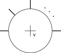
Figure 1: Tadpole calculation of superpotential

Multiple trace operators would then correspond to string loop diagrams, and are therefore suppressed by powers of $g_{str}$. It is not clear that the string generates these effects perturbatively, but to avoid them we could work at weak string coupling. It is also possible that a non-perturbative non-renormalization theorem might keep multiple trace operators equal to zero, at least up to some number of derivatives.

3 Non-Commutative Algebraic Geometry

3.1 Overview

As discussed above, we usually think of the moduli spaces of vacua as varieties, namely commutative algebraic geometric objects. Because the $F$- and $D$-term constraints may be recast in matrix form, it is more convenient to think of the same space as a non-commutative object. Although the physical problem to solve is the same and the space of solutions is the same, the non-commutative interpretation invokes extra structure (namely, the commutative algebra of individual matrix elements is organized into the non-commutative algebra of matrices). Because $D$-brane solutions are associated with algebraic geometric objects in general[35] (and see [36] for a review), we need a formulation of non-commutative algebraic geometry which captures $D$-brane physics correctly.

Several different versions of non-commutative algebraic geometry have been discussed in the mathematics literature[25, 26, 27], but none of these seem natural in the present context. In this section, our aim is to describe a definition of algebraic geometry appropriate to the moduli spaces of vacua of $D$-branes in the field theory limit.

We want to understand the holomorphic structure of the moduli space, so we will only concentrate on the $F$-term equations and will assume that given a solution to the $F$-terms, there is a solution to the $D$-term equations. From the physics point of view, we confine ourselves to those properties which are protected by supersymmetry; from a mathematical viewpoint, these are holomorphic structures and can be described in terms of algebraic geometry. Ordinarily, non-commutative geometries are related to $C^{*}$-algebras[37], which include the adjoint operation; this is not a natural operation in a holomorphic framework, and we will discard it for the considerations of this paper. In supersymmetric theories, the holomorphic and anti-holomorphic features couple only through $D$-terms, and these effects are in general not protected by supersymmetry. In discarding the $D$-terms, we lose information about the metric in moduli space, but not topological features. Thus we need a framework where we can do non-commutative algebraic geometry without $C^{*}$-algebras.

In the rest of this subsection, we give a brief outline of the mathematics involved, and its physical interpretations. For the reader who wishes to skip the details of the mathematics, this overview should suffice, and one may proceed to Section 4.

The building blocks for solutions are the finite dimensional irreducible representations of the algebra, as in eq. (9). In the non-commutative algebraic geometry that we will describe, these are defined to be points[37, 40]. In matrix theory, non-commuting matrices are interpreted as extended objects; here, these are considered point-like objects. In orbifold theories, D-branes in the bulk are also considered to be point-like even though they can be built out of fractional branes.

In our construction the center (the commutative sub-algebra of the Casimir operators) plays a pivotal role. In particular, one expects[21] that for a given background in string theory, there are two descriptions, a commutative version relevant to closed strings and a non-commutative version for open strings. In our best-understood examples, the commutative space is the algebraic geometry associated to the center. By Schur’s lemma, on every irreducible representation the Casimirs are proportional to the identity. Because of this, one finds a map between non-commutative points and commutative points. For “good” algebras, the non-commutative geometry covers the commutative geometry; in this case, we will say that the non-commutative algebra is semi-classical. In this case we can think of the commutative space as a coarse-grained version of the full non-commutative space. For semi-classical algebras, our interpretation of irreducible representations as points is equivalent to the point-like properties of $D$-branes in orbifolds. In other cases, the non-commutative geometry may have little relation to the commutative geometry and it is not clear that one should interpret the $D$-brane states as pointlike.

A general solution of the $F$-term constraints is a direct sum of irreducible representations, and thus the natural non-commutative structure is an unordered finite collection of points. For commutative algebras, we would interpret this as a symmetric product space, and we will carry over this name in the non-commutative case. This symmetric product structure leads directly to an interpretation of $D$-brane fractionation at a singularity, whereby an irreducible representation can be continuously deformed and becomes reducible at a certain point. In this sense, in the non-commutative version, single-particle and multi-particle states are continuously connected. In commutative geometry on the other hand, this process would be singular.

The remainder of the formal discussion deals with an extension of this construction to subvarieties, sheaves, and the algebraic K-theory of the ring, relevant to an understanding of extended $D$-branes. The discussion presented here lays the outline for non-commutative algebraic geometry; a full account will appear elsewhere[38].

3.2 Preliminaries: Points and Topology

Consider an associative algebra ${\cal A}$ over the complex numbers ${\mathbb{C}}$, generated by a set of operators subject to some relations. (In all the examples we consider, we will have three generators and a set of quadratic relations.) As is standard, the non-commutative algebra should be thought of as a ring of functions on some affine non-commutative space[37]. Ring homomorphisms should correspond to holomorphic maps between affine non-commutative geometries. We will assume that all rings are Noetherian (so that any ideal always has a finite basis) and that the algebra is polynomial.

Given the matrix equations (6)–(8), we want to find solutions in terms of $M\times M$ matrices (with unspecified $M$). That is, we are interested in representations of the algebra, and we will assign a geometrical space to these solutions.

An element $a\in{\cal A}$ is central if it commutes with every other element in ${\cal A}$; that is, $a$ is a Casimir of the algebra. We usually think of the Casimir operators as sufficient to define a representation (e.g., as in the finite dimensional representations of $SL(2,{\mathbb{C}})$) and thus will pay particular attention to the center of the algebra, denoted ${\cal Z}{\cal A}$.

Since ${\cal Z}{\cal A}$ is commutative, we can associate an ordinary commutative space to it, which is the general philosophy behind algebraic geometry (see for example, Ref. [39]). We interpret the center of the algebra as a coarse description of the full non-commutative geometry. The picture we have is that there is a map between the non-commutative geometry to the commutative one which forgets some of the structure (namely the functions that don’t commute). The natural inclusion ${\it i}:{\cal Z}{\cal A}\to{\cal A}$ is to be thought of as the pullback of functions from the commutative space to the non-commutative space.

To describe the non-commutative space, we need to define the notions of points and open sets and to impose a topology. Loosely speaking, a point will be a solution of the constraint equations in finite matrices (just as points in varieties are solutions of the equations defining the variety). In commutative algebra, points are interpreted as maximal ideals of the algebra, and we want to incorporate both of these notions in our definition of a point.

Let us now be precise. A representation $R$ of dimension $M$ of the algebra ${\cal A}$ is an algebra homomorphism $\mu$ from ${\cal A}$ to the algebra of $M\times M$ matrices (i.e., $\mu$ respects the addition, product, and multiplication by scalars). For the map to be well defined, the relations ($F$-term constraints) must be satisfied in terms of the $M\times M$ matrices.

A representation is irreducible if there is no linear subspace of ${\mathbb{C}}^{M}$ which is invariant under multiplication by all the elements of the image of the algebra $\mu({\cal A})$. The representation is reducible otherwise. If a representation is irreducible, then the map is such that we have an exact sequence

$${\cal A}\stackrel{{\scriptstyle\mu}}{{\to}}M_{M}({\mathbb{C}})\to 0$$ (10)

with the map $\mu$ defined by the representation of the algebra. The kernel of this map is a double-sided ideal ${\cal I}$ of ${\cal A}$ to which the representation is associated, and we have the isomorphism

$${\cal A}/{\cal I}\sim M_{M}({\mathbb{C}}).$$ (11)

This isomorphism is non-canonical (two representations are identified if they lie in the same orbit of the group $GL(M,{\mathbb{C}})$ by similarity transformations).

The space associated to an algebra is constructed from the irreducible representations of ${\cal A}$ as follows. To each irreducible representation of finite dimension $M$, there is an associated ideal in the algebra ${\cal A}$, namely the ideal ${\cal I}=\ker(\mu)$. ${\cal I}$ is a double-sided maximal ideal and is declared to be a point. This definition is borrowed from [37, 40], but without the $C^{*}$-algebra framework. In general, one would also allow infinite dimensional representations of the algebra; in that case, we would need some sense of convergence for sequences. For our physical problem, we are interested only in finite dimensional representations, and so we will simply discard this possibility. As a result, we have a space which is better behaved from an algebraic standpoint. Irreducible representations are considered equivalent if they are related by a change of basis (i.e., by orbits of the group $GL(M,{\mathbb{C}})$). This equivalence is the fact that we have in supersymmetric field theories a complexified gauge group, and each point has an associated maximal double-sided ideal ${\cal I}$ of the algebra ${\cal A}$ such that ${\cal A}/{\cal I}$ is non-canonically isomorphic to the algebra of $M\times M$ matrices. The variety associated to ${\cal A}$ will be labeled ${\cal M}_{\cal A}$.

A closed set is defined in terms of an arbitrary double-sided ideal ${\cal I}^{\prime}$ in ${\cal A}$, as one does to define the Zariski topology of a space. A closed set is the collection of points (given by maximal ideals ${\cal I}$) which contain ${\cal I}^{\prime}$. By definition, points are closed sets, as one takes the maximal ideal ${\cal I}$ associated to the point.

The union of two closed sets corresponds to the double-sided ideal ${\cal I}={\cal I}_{1}\cap{\cal I}_{2}$, and the intersection of two closed sets corresponds to the double-sided ideal ${\cal I}_{1}+{\cal I}_{2}$, which is the direct sum of the ideals. Indeed, direct sums may be extended to an infinite number of ideals, so arbitrary intersections and finite unions of closed sets are closed and define a topology on the set of points. This should be thought of as a model for the definition of the geometry, and the construction mimics the construction of algebraic varieties over ${\mathbb{C}}$ as much as possible.

Note that the definition of a point has the following technical property. A point is Morita-equivalent to a point in a commutative algebraic variety. This is important for K-theory considerations, which we return to in a later subsection.

3.3 Naturalness of Symmetric Spaces

So far, we have defined a non-commutative space together with some topology. Given these definitions, additional structure naturally emerges, as we now discuss.

When one has the ring of functions of a variety, one can pull back functions between maps of varieties. Thus, a map between non-commutative spaces will correspond to ring homomorphisms. If we take two rings ${\cal A}$ and ${\cal B}$ and consider a ring homomorphism $\varphi:{\cal A}\to{\cal B}$, it will correspond to a continuous map from ${\cal M}_{\cal B}\to{\cal M}_{\cal A}$.

Now consider a point $x\in{\cal M}_{{\cal B}}$. By construction, it corresponds to an irreducible representation of ${\cal B}$ in $M\times M$ matrices for some $M$. We label the corresponding representation $r_{x}$, i.e, a homomorphism $\mu_{x}:{\cal B}\to M_{M}({\mathbb{C}})$. Thus we have a diagram of maps

$${\cal A}\stackrel{{\scriptstyle\varphi}}{{\to}}{\cal B}\stackrel{{\scriptstyle\mu_{x}}}{{\to}}M_{M}({\mathbb{C}}).$$ (12)

We wish to find the image of the point $x$ in ${\cal M}_{\cal A}$. By composing arrows, we get a natural representation of ${\cal A}$ in the ring of $M\times M$ matrices. The natural image of $x$ is the kernel of the composition map, but it is important to note that the corresponding $M\times M$ representation of ${\cal A}$ might be reducible. In general, to find irreducible representations associated to a given reducible one, we need to consider the composition series of the representation $R$.

That is, given a reducible representation $R$, there is an invariant linear subspace $R^{\prime}$, and we have an exact sequence of vector spaces:

$$0\to R^{\prime}\to R\to R/R^{\prime}\to 0.$$ (13)

By construction the dimensions of $R^{\prime}$ and $R/R^{\prime}$ are smaller than that of $R$. If any of $R^{\prime}$, $R/R^{\prime}$ is reducible, we repeat the procedure. Eventually, we obtain a collection of irreducible representations of ${\cal A}$, and any two such decompositions contain the same irreducibles.

The image of $x$ should be considered a positive sum of points in ${\cal M}_{\cal A}$ with multiplicities given by the number of times a particular irreducible representation of ${\cal B}$ appears. Thus the map is multivalued, given the description used so far. If we wish to make such maps single-valued, we can either restrict the choice of maps, or modify the definition of a point. The latter possibility is most natural, and there is an obvious choice. We should consider instead a new space consisting of the free sums of points with coefficients in ${\mathbb{Z}}^{+}$. These sums of points are generated by the points of ${\cal M}$ such that the sums are finite. We should consider the maps between two such spaces as linear transformations between the two formal sums. Notice that the formal positive sums of $n$ points in a commutative variety ${\cal M}$ corresponds to the symmetric product ${\cal M}^{n}/S_{n}$. Hence the natural object to understand in this version of non-commutative algebraic geometry is the symmetric product of the space ${\cal M}_{\cal A}$. This is also the framework necessary for matrix theory and matrix string theory[34, 41], and this is why we find it a very appealing aspect of the construction. We will denote this symmetric product space by ${\cal S}{\cal M}_{\cal A}$. ${\cal M}_{\cal A}$ is a subset of its symmetric space, and it is the set which generates the formal sums.

There is a grading present here which gives a notion of the degree of a point, which we denote $\deg(x)$. There is a natural map from the formal sums of points to ${\mathbb{Z}}$; namely, for each irreducible representation $x\in{\cal M}_{\cal A}$, we consider the map that assigns to $x$ the dimension of the representation that $x$ is associated with (that is, the character ${\rm tr}_{\mu_{x}}1$). This extends by linearity to the symmetric product space, and the maps between the sums of points are such that they are degree-preserving. Indeed, given any function on the space (an element of the ring $a\in{\cal A}$), we consider the invariant of the function $a$ at the point $x$, ${\rm tr}_{\mu_{x}}a$. The trace is linear, and independent of the choice of basis for the local matrix ring and can therefore be extended to direct sums of representations (i.e., to the space ${\cal S}{\cal M}_{\cal A}$).

Each positive sum of points of ${\cal M}_{\cal A}$ is associated with a representation of the ring ${\cal A}$, which is the direct sum of irreducible representations. To each element in the ring, we associate a character in the representation. Consider the vector space associated to a representation on which the matrix ring acts as a left module of the ring of functions. Because the associated representations of points are only well defined up to conjugation, we should impose the same constraint on the modules; namely, we want isomorphism classes of modules for the ring ${\cal A}$. This is very reminiscent of algebraic K-theory, and we will expand on this idea later, making the connection precise.

Now, although we have found it natural to extend ${\cal M}_{\cal A}$ to ${\cal S}{\cal M}_{\cal A}$, it is not the case that ${\cal S}{\cal M}_{\cal A}$ automatically inherits a topology from that of ${\cal M}_{\cal A}$. Rather, we should repeat the construction of a Zariski topology, by giving a definition of closed sets. For any function $a\in{\cal A}$ and for every complex number $z$, we define the following set

$${\cal Z}=\{p\in{\cal S}{\cal M}_{\cal A}|{\rm tr}_{R_{p}}(a)=z\}$$ (14)

to be closed. These sets form a basis of closed sets for the topology of ${\cal S}{\cal M}_{\cal A}$. This topology coincides with the natural topology in the commutative algebra of functions generated by traces of operators, which are the polynomials in the gauge invariant superfields, and thus gives us the same topological information that we would want for the moduli space if we just consider the ring of holomorphic functions on the moduli space with values in ${\mathbb{C}}$. For later use, we define the support of a character as

$$Supp({\rm tr}\ a)=\overline{\left\{p\in{\cal S}{\cal M}_{\cal A}|{\rm tr}_{R_{p}}a\neq 0\right\}}$$ (15)

where the overline denotes the closure operation.

We would like to be able to say that the space is foliated by sets of degree $m$ (which will count the $D$-brane charge of the point). Because the Zariski topology is coarse, we must then additionally declare that the sets defined by $\deg(x)=m$ are both open and closed.

Now recall that for two different points in an algebraic variety $V$, there is some function on the variety which distinguishes them. Only a finite number of these functions is needed to determine a point exactly; the ring of polynomials (with relations) is finitely generated. This construction is also sufficient to determine a collection of $n$ unordered points of the variety. By examining $n$th order polynomials in a function $f$, we can determine the values that $f$ takes at the $n$ points. If the values are different for all the points for some function $f$, then one can use $f$ as a coordinate, and one has a collection of $n$ non-overlapping algebraic subsets of $V$, with one point chosen from each one. Thus we can construct a function which vanishes at all but one of the subsets, which we call $f_{1}$ and by multiplying $f_{1}$ by all the basis functions of the ring associated to $V$, we can identify one of the points. The procedure can be repeated if no one function is able to tell them all apart, and then we get the multiplicities of the points.

In the non-commutative case, we say that we can always distinguish two irreducible representations by some collection of characters (traces) of the ring ${\cal A}$. Thus there is a given finite number of functions with which we can distinguish $n$ points.

Recall that we wish to think of the non-commutative symmetric space as a refined version of the commutative space. Topologically, the two spaces are the same. It is clear that, at least locally, given the characters of enough elements of the ring, we can fully reconstruct a representation by holomorphic matrices on the commuting variables. This endows the symmetric space locally with a holomorphic vector bundle structure.

3.4 The Role of the Center

Now let us apply the above construction to maps between the spaces ${\cal S}{\cal M}_{\cal A}$ and ${\cal S}{\cal M}_{{\cal Z}{\cal A}}$. Consider in particular the inclusion map ${\cal Z}{\cal A}\to{\cal A}$, which is the pullback of functions on ${\cal M}_{{\cal Z}{\cal A}}$ to ${\cal M}_{\cal A}$.

We want to know the image of a point $p$ in ${\cal M}_{\cal A}$. Given the point $p$, there is an associated $M$-dimensional irreducible representation $\mu_{p}$. Consider composing the maps ${\cal Z}{\cal A}\stackrel{{\scriptstyle{\it i}}}{{\to}}{\cal A}\stackrel{{\scriptstyle\mu_{p}}}{{\to}}M_{M}({\mathbb{C}})$. As the last map is onto, if $a\in{\cal Z}{\cal A}$, it commutes in the image of the composition of maps and by Schur’s lemma is proportional to the identity. The representation associated to $p$ splits into $M$ identical copies of a single representation of ${\cal Z}{\cal A}$, namely, into $M$ copies of a single point. We write this as

$$p\mapsto M\bar{p}$$ (16)

where $\bar{p}$ is the associated maximal ideal of ${\cal Z}{\cal A}$, which is the kernel of the inclusion map.

We will call this the natural map, as it respects degree. Notice that we can also define a map between the symmetric spaces $p\mapsto\bar{p}$ which forgets the degree. In this case, the image of a point is a point, so we can restrict the maps to ${\cal M}_{\cal A}$ and ${\cal M}_{{\cal Z}{\cal A}}$. We will call this the forgetful map.

The center of the algebra will play an important role in the physics. We wish to restrict the maps between rings ${\cal A}$ and ${\cal B}$ in the following way. Note that we have the following diagrams

$$\begin{matrix}{\cal A}&\rightarrow&{\cal B}\\ \uparrow&&\uparrow\\ {\cal Z}{\cal A}&&{\cal Z}{\cal B}\end{matrix}\ \ \ \ \ \ \ \ \ \ \ \ \begin{matrix}{\cal S}{\cal M}_{\cal B}&\rightarrow&{\cal S}{\cal M}_{\cal A}\\ \downarrow&&\downarrow\\ {\cal S}{\cal M}_{{\cal Z}{\cal B}}&&{\cal S}{\cal M}_{{\cal Z}{\cal A}}\end{matrix}$$ (17)

We require that these diagrams be commutative; namely, the ring homomorphism ${\cal A}\to{\cal B}$ induces a map ${\cal Z}{\cal A}\to{\cal Z}{\cal B}$, and consequently ${\cal S}{\cal M}_{{\cal Z}{\cal B}}\rightarrow{\cal S}{\cal M}_{{\cal Z}{\cal A}}$. Thus, we want the map to be such that central elements are central not just in the subalgebra of the image of ${\cal A}$ but in the algebra ${\cal B}$ itself.

Now we are at a point where we can build a category for the non-commutative algebraic geometry. The objects will be rings $({\cal A})$ with the center identified and the inclusion map singled out. The allowed maps between rings are such that they produce commuting squares

$$\begin{matrix}{\cal A}&\rightarrow&{\cal B}\\ \uparrow&&\uparrow\\ {\cal Z}{\cal A}&\rightarrow&{\cal Z}{\cal B}\end{matrix}$$ (18)

with the upwards arrows the natural inclusion maps.

The non-commutative space is a contravariant functor from this category of rings to a category of ‘symmetric spaces’ as we have defined previously (including the degree map and the degree-preserving property). Thus we have the diagram

$$\begin{matrix}{\cal S}{\cal M}_{\cal B}&\rightarrow&{\cal S}{\cal M}_{\cal A}\\ \downarrow&&\downarrow\\ {\cal S}{\cal M}_{{\cal Z}{\cal B}}&\rightarrow&{\cal S}{\cal M}_{{\cal Z}{\cal A}}\end{matrix}$$ (19)

Together with the center preserving property, the forgetful map induces

$${\cal M}_{{\cal Z}{\cal B}}\to{\cal M}_{{\cal Z}{\cal A}}.$$ (20)

This is a map of commutative algebraic varieties, to which we can apply intuition. It is also clear that this map between varieties has all the data required to specify the map between their symmetric spaces. With the topology of these spaces, all the arrows are continuous maps, and composition of maps is a map that respects the properties of the category.

To make a full connection with algebraic geometry, we want to be able to glue rings on open sets. This should be done by a process of localization. These details will be left for a future publication[38].

It is useful to notice that all the irreducible representations of the center may not appear when we consider the projection map, ${\cal S}{\cal M}_{\cal A}\to{\cal S}{\cal M}_{{\cal Z}{\cal A}}$. If most do appear, then we will call the algebra semi-classical, because to the points in the variety associated to the center, we can lift to points in the non-commutative variety. The non-commutative variety covers the commutative one and this notion will be important from several perspectives below. In particular, there are applications involving $D$-branes in which phenomena on orbifold spaces are more precisely described by non-commutative geometry.

3.5 $D$-brane Fractionation

The technology developed so far contains some interesting aspects of $D$-brane physics. In particular, we wish to show that a $D$-brane fractionates as we move to a singular point of a non-commutative algebraic variety. In fact we define singular points via this process of fractionation. We will consider in this subsection $D$-branes which correspond to points in ${\cal M}_{\cal A}$, and the degree of the point is identified with the $D$-brane charge. The moduli space of supersymmetric configurations of $D$-branes is identified with ${\cal S}{\cal M}_{\cal A}$.

Let $R$ be an irreducible representation of dimension $M$ in ${\cal A}$. Consider its image in ${\cal S}{\cal M}_{\cal A}$ as a single point of degree $M$. Because ${\cal S}{\cal M}_{\cal A}$ is an algebraic variety, it will consist of several components or branches. The branch of ${\cal S}{\cal M}_{\cal A}$ where $R$ is located is a closed set of some complex dimension $d$ which is not a closed subset of any set with larger local dimension.

On this branch, we can define a local function which is the dimension of the commutant ${\cal Z}R$ of the representation $R$. As we move along the branch, this function is semi-continuous—it may jump in value on closed sets.

Clearly, the sets with $\dim({\cal Z}R)>1$ are closed. In this case, we have at least two linearly independent matrices which commute with everything in the image of ${\cal A}$, and thus the representation cannot be irreducible. For irreducible representations, $\dim({\cal Z}R)$ must be unity. Thus, if we start at a point on a branch of the variety that is irreducible, as we continuously deform along it, we can reach a special point as a limit point, where the representation becomes reducible.

Parametrize this deformation by $z$; on the symmetric product space we have the process

$$\lim_{z\to z_{0}}x(z)=x_{1}+\dots+x_{n}$$ (21)

if $z_{0}$ is such a limit point, and where $n$ is the number of irreducible representations that $R(z)$ splits into. Then, we say that the $D$-brane has fractionated, and there may be additional branches that intersect that point, corresponding to separating the fractional branes.

From the point of view of the center of the algebra, each element is proportional to the identity throughout the branch of the symmetric space, and thus there is no splitting seen in ${\cal S}{\cal M}_{{\cal Z}{\cal A}}$. In this sense, the non-commutative geometry is a finer description of the $D$-brane moduli space than the associated commutative geometry.

In the cases where there are branches corresponding to separating the branes at $z_{0}$, if we think in terms of the forgetful map, we would have a single point splitting into $n$ points. From the point of view of the commutative algebraic variety, there is a jump in dimension as we go from one branch to the next; this is naturally associated with a singularity. We will see explicit examples of this in Section 4.

3.6 Higher dimensional branes

So far, we have considered $D$-branes that are point-like on the moduli space. We would also like to identify more general brane configurations, such as those wrapped on holomorphic subspaces; hence we need to construct such objects algebraically. It is natural to consider coherent sheaves[35]: these are the modules over the ring ${\cal A}$ which locally have a finite presentation and are well-behaved when considered from the commutative standpoint. Extended BPS brane solutions usually correspond to stable sheaves, given some appropriate notion of stability. Moreover, they are also well-behaved as far as K-theory is concerned. However, in order to define these structures, it is most convenient to have a semi-classical ring. This does not mean that there is no useful way to define these objects for more general rings, but on some rings where the points are discrete there is no obvious notion of an extended object. For the rest of this section, we will assume that we are indeed working in a semi-classical ring.

As the ring is semi-classical, we can try to construct extended objects by first building them over a holomorphic subspace of the commutative structure, and then try to lift them up to the non-commutative geometry. In the commutative case, a $D$-brane corresponds to a coherent sheaf with support on a commutative subvariety. For any notion of non-commutative sheaf, it must be the case that it is also a coherent sheaf over the commutative ring. In the commutative case, the $D$-brane is a module over the ring ${\cal Z}{\cal A}$, such that if ${\cal Z}{\cal I}$ is the ideal corresponding to the support of the sheaf, the module action of ${\cal Z}{\cal A}$ factors through ${\cal Z}{\cal A}/{\cal Z}{\cal I}$, which is considered to be the coordinate ring of the closed set associated to the ideal ${\cal Z}{\cal I}$.

On ‘good’ varieties we always have a presentation of a sheaf ${\cal S}$ as the right-hand term of some exact sequence

$${\cal Z}{\cal A}^{m}\to{\cal Z}{\cal A}^{n}\to{\cal S}\to 0$$ (22)

that is, as a module with $n$ generators with relations induced by the images of ${\cal Z}{\cal A}^{m}$.

We want to mimic this construction for the non-commutative version of the $D$-brane. Note that in the non-commutative case, we have a choice of left-, right- or bi-modules of the algebra ${\cal A}$. However, physically, we need to consider only bi-modules, as both ends of open strings end on a $D$-brane. That is, gauge transformations (which act locally) act both on the left and right, and therefore the algebra has to be able to accommodate both types of actions on the modules. Referring to the bi-module as ${\cal R}$, we want them to arise from exact sequences

$${\cal A}^{m}\to{\cal A}^{n}\to{\cal R}\to 0$$ (23)

in analogy to eq. (22). This defines locally the coherent sheaves over ${\cal A}$.

The annihilator of a bi-module ${\cal R}$ is defined as the largest ideal ${\cal I}$ of ${\cal A}$ such that ${\cal I}{\cal R}={\cal R}{\cal I}=0$. This is a double-sided ideal, and thus defines a closed set, in the topology of ${\cal M}_{\cal A}$. For any point $p$ in ${\cal M}_{\cal A}$ which does not belong to ${\cal I}$, ${\cal I}+{\cal I}_{p}$ is equal to ${\cal A}$ (because ${\cal I}_{p}$ is maximal). We will refer to this ideal ${\cal I}$ as $\hbox{Ann}({\cal R})$.

We can find how a bi-module restricts to a closed subset (described by an ideal ${\cal I}$) by noticing that if ${\cal R}$ is a bi-module over ${\cal A}$, then ${\cal R}/({\cal I}{\cal R}+{\cal R}{\cal I})$ is a bi-module over ${\cal A}/{\cal I}$. For maximal ${\cal I}_{p}$ the restriction is zero if $\hbox{Ann}({\cal R})\subset\kern-8.99994pt/\kern 3.00003pt{\cal I}_{p}$. We can define the support of a sheaf to be the set of points such that

$$\hbox{Ann}({\cal R})\subset{\cal I}_{p}.$$ (24)

We study the sheaves locally by restricting to a point. We will look at two different notions of the rank of a sheaf. Each non-commutative point is Morita equivalent to a commutative point. This tells us that modules over the functions restricted to a point $p$ (the ring of $n\times n$ matrices) behave just as vector spaces over ${\mathbb{C}}$. Thus the sheaf restricted to a point is a bi-module over the ring of $\deg(p)\times\deg(p)$ matrices, and thus ${\cal R}|_{p}$ is isomorphic to $\left({\cal A}|_{p}\right)^{k}$, for some $k$. One possible definition of non-commutative rank of a sheaf at the point $p$ is just $k$. However, as seen from the commutative standpoint, the dimension of the representation associated to $\left({\cal A}|_{p}\right)^{k}$ is $k\deg p$, and this then serves as another definition of rank, which we will refer to as the commutative rank.

As usual, rank is upper semi-continuous (the points where $rank({\cal R})|_{p}>m$ form a closed set). The rank can jump in value on some closed subset, and this is interpreted in terms of an additional $D$-brane of smaller dimension stuck to the brane, as follows from the anomalous couplings of $D$-branes[42].

For the non-commutative points, we have to take into account that a limit set of a collection of points might be a sum of points. Consider the trivial bi-module of ${\cal A}$, namely ${\cal A}$. The non-commutative rank (equal to 1) does not jump under the fractionation process. The commutative rank on the other hand, does jump at this singularity. The non-commutative rank then is the natural definition of rank for non-commutative algebras.

Note, however, that if we look just at the center ${\cal Z}{\cal A}$, the commutative rank is the natural definition, as it does not jump in a splitting process; we have

$$\deg(p)=\sum_{i}\deg{p_{i}}.$$ (25)

With these definitions, a $D$-brane is a coherent sheaf over both the non-commutative ring and the commutative sub-ring.

3.7 K-theory interpretation

We have seen that our approach to non-commutative geometry has led us to some definitions of $D$-brane states. We now want to add $K$-theory to the discussion. Because we have a ring and we have bi-modules, we get automatically a K-theory associated to this structure, namely, the algebraic K-theory of the ring ${\cal A}$ (see [43] for example). From a mathematical standpoint this is review material, and we will just glimpse at the dynamics in terms of brane-antibrane systems[44, 23].

Indeed, let us start with the construction of the symmetric space. We had formal sums of points which makes the non-commutative geometry a semigroup. We can make it into a group by adding minus signs, and a rule for cancellation. This group is the equivalent of zero-chains of points.

Now, the idea of the group structure is to understand that $p+(-p)=0$. So if $p$ is a point, we interpret it as a point like $D$-brane, and $-p$ is an anti-$D$-brane. The cancellation law of the group is the statement that a $D$-brane anti-$D$-brane pair can be created from the vacuum.

Given these minus signs, the degree function now maps to the integers and gives us an invariant, which is a group homomorphism of Abelian groups, $\deg:\oplus p\to{\mathbb{Z}}$. This number is the total $D$-brane charge of a configuration. It is possible to give a topology to finite formal sums of points by the same construction we used based on characters. The extra ingredient to make $p-p=0$ is to add minus signs for the anti-$D$-brane.

Thus dynamically $p-p=0$ is the statement that any character of $p-p$ is the same as a character of zero, and thus the configurations are connected. When we create a $D$-brane anti-D brane pair we can separate them if there are moduli available, and thus the process is continuous in this topology. Dynamical information would include the energy required for this process. (A generic point is such that this energy is much less than the energy required to move off of the moduli space of sums of points. A non-generic point is where the mass matrix has zero eigenvalues.)

The idea now is to define the K-theory of points as a homotopy invariant which respects the additivity of branes. On one hand, we have the mathematical definition of the $K^{p}_{0}$-theory of points as the formal abelian group of homotopy classes of finite dimensional representations of the algebra ${\cal A}$, such that if $a,b$ are such representations, then the K-theory classes associated to $a\oplus b,a,b$ satisfy

$$K(a\oplus b)=K(a)+K(b)$$ (26)

and if one has a homotopy between the two representations $a\sim b$, then $K(a)=K(b)$. Indeed, to the point $p$ we associate the bi-module ${\cal A}|_{p}$, and this is thought of as the skyscraper sheaf over $p$. With this extra relation this is part of the K-theory of bi-modules of the algebra.

The other way to define K-theory is to say $K(a)=K(b)$ if there is $c$ such that $a\oplus c\sim b\oplus c$. Both of these definitions agree.

There are a few possible choices of K-theory depending on the type of modules one chooses. As we have stated above, in this paper we are interested in finitely presented bi-modules over the ring ${\cal A}$. Generically, one defines the K-theory associated to projective bi-modules of the algebra. The K-theory of projective bi-modules is the same as the K-theory of finitely presented bi-modules as long as every bi-module admits a projective resolution (this is true, for example, in smooth manifolds where every vector bundle is projective over the coordinate ring of the manifold). Thus, as long as there is a long exact sequence

$$0\to P_{1}\to\dots P_{k}\to M\to 0$$ (27)

with the $P_{i}$ projective, then the K-theory class of $M$ is defined. This requires the ring to be regular. Whether or not we will always get regular rings in string theory in this framework is not clear. (Singular varieties are not regular as commutative algebras, yet they do appear in string theory.)

The $K_{0}$-theory is defined as the set of formal sums of bi-modules modulo homotopy, and modulo the relations

$$K(b)=K(a)+K(c)$$ (28)

whenever there is a short exact sequence

$$0\to a\to b\to c\to 0$$ (29)

of the bi-modules we have described. We think of this as the statement that $b-a-c=0$.

If a module $M$ admits a projective resolution as in (27) then it is a simple exercise to show that

$$K(P_{1})-K(P_{2})+\dots-(-1)^{k}K(P_{k})+(-1)^{k}K(M)=0$$ (30)

Physically, we say the dynamics of brane-antibrane configurations is such that given a short exact sequence (29), the process

$$X\to X\pm a\mp b\pm c$$ (31)

is allowed, namely $a-b+c$ carries no $D$-brane charge. In particular, the exact sequence

$$0\to a\to a\to 0\to 0$$ (32)

will allow any of the two processes

$$X\to X+a+(-a)\to X$$ (33)

which correspond to the creation of brane-antibrane pairs. Of course, the real dynamics of these processes is not available to us, but the topology of allowed transitions is correctly reproduced.

Note that taking tensor products of bi-modules is locally a good operation (at each point we are taking a tensor product of finite dimensional spaces, and we get a finite dimensional space). Thus the K-theory is not just an additive group but we have a multiplication as well, and this permits us to do intersection theory (that is, we can count strings when branes intersect). This type of information can often be enough to calculate topological quantities in string theory.

As a final comment, we have to give some warnings to the reader. The K-theory we have constructed here is the one associated to the holomorphic algebra, and thus is a version which is relevant for the algebraic geometry. This K-theory is an invariant of a holomorphic space which is much finer than the topological K-theory, and thus contains a lot more information. The K-theory which is relevant for $D$-brane charge is the one associated to both the holomorphic and anti-holomorphic structures, namely, the K-theory of a ${\mathbb{C}}^{*}$ algebra of which ${\cal A}$ is a subalgebra. This ${\mathbb{C}}^{*}$ algebra includes the D-term constraints, and by theorems on existence of solutions[33] the geometric space associated to the ${\mathbb{C}}^{*}$ algebra has just as many non-commutative points as the one associated to ${\cal A}$. So just as in commutative cases, the non-commutative holomorphic data parametrize the full variety. The K-theory of the two algebras does differ. The holomorphic K-theory is therefore more appropriate to count BPS states, rather than just account for the $D$-brane charge.

This is the end of the mathematical preliminaries. We believe that we have presented a fairly general account of how applications of these techniques might be pursued. We will see that this approach is not just a big machine which describes things we already knew in a complicated manner. Indeed, once we have examined the examples in the next sections, it will be clear that the formulation brings sound intuition and gives a very nice picture of how string geometry behaves.

4 Examples

In this section, we consider a variety of examples in order to build a picture of the generic behavior of the geometry, which is not present in the simplest case. The presentation is given in terms of the language of Section 3; the reader will find it necessary to read, at least, the overview in Section 3.1. In the first few examples, we first calculate the commutative algebra of the center which reproduces the string geometry associated with the field theory (e.g., the orbifold). We then attempt to build the irreducible representations of the full non-commutative algebra by exploiting knowledge of the center. A posteriori, the structures that we find here and the relations to the physics of $D$-branes in these geometries discussed in later sections, motivates the formal constructions of Section 3. In more general examples, the calculation of the center is difficult, and we present only partial results.

4.1 Orbifolds with discrete torsion: the $q$-deformation

Our first example to study will be orbifolds with discrete torsion. In particular, we consider the orbifold ${\mathbb{C}}^{3}/{\mathbb{Z}}_{n}\times{\mathbb{Z}}_{n}$ with maximal discrete torsion. To construct the low energy effective field theory of a point-like brane one can use a quiver construction[45] with projective representations of the orbifold group[6]. The use of projective representations was justified in Ref. [46]. The algebraic variety associated to the orbifold singularity is given by the solutions of one complex equation in four variables,

$$xyz=w^{n}.$$ (34)

As Douglas showed[6, 47], the theory has $N=1$ supersymmetry in four dimensions and consists of a quiver with one node, gauge group $U(M)$, three adjoint superfields and a superpotential

$$W_{q}={\rm tr}(\phi_{1}\phi_{2}\phi_{3})-q{\rm tr}(\phi_{2}\phi_{1}\phi_{3})$$ (35)

with $q$ a primitive $n$-th root of unity. This theory can be obtained by a marginal deformation of the $N=4$ supersymmetric field theory as shown in [1, 7], and as such, when studied under the AdS/CFT correspondence, displays a duality between two totally different near-horizon geometries, describing the same field theory.

The $F$-term constraints are given by

$$\phi_{1}\phi_{2}-q\phi_{2}\phi_{1} = 0$$ (36)

$$\phi_{2}\phi_{3}-q\phi_{3}\phi_{2} = 0$$ (37)

$$\phi_{3}\phi_{1}-q\phi_{1}\phi_{3} = 0$$ (38)

We will often write these using the $q$-commutator notation $\left[\phi_{1},\phi_{2}\right]_{q}=0$, etc. These equations are exactly the type of relations seen in the algebras related to quantum planes[18], and have been very well studied. Let us analyze the algebra using the tools described in Section 3.

Because of the $F$-term constraints, we can always write any monomial in ‘standard order’

$$\phi_{1}^{k_{1}}\phi_{2}^{k_{2}}\phi_{3}^{k_{3}}.$$ (39)

We associate to this monomial the vector $(k_{1},k_{2},k_{3})$.

Note that if an element commutes with $\phi_{1},\phi_{2},\phi_{3}$, then it commutes with any of the monomials, and thus is an element of the center of the algebra. Monomials may be multiplied, and up to phases, we have

$$(k_{1},k_{2},k_{3}).(s_{1},s_{2},s_{3})\sim(k_{1}+s_{1},k_{2}+s_{2},k_{3}+s_{3}).$$ (40)

Because of the phases, generators of the center are monomials.

It is easy to see that $(k_{1},k_{2},k_{3}).\phi_{1}=\phi_{1}.(k_{1},k_{2},k_{3})q^{k_{3}-k_{2}}$, so that $k_{3}=k_{2}\mod n$ for $(k_{1},k_{2},k_{3})$ to be in the center. Similarly one proves $k_{2}=k_{1}\mod n$ and thus the center is given by the condition

$${\cal Z}{\cal A}=\left\{\sum(k_{1},k_{2},k_{3})\big{|}k_{1}=k_{2}=k_{3}\mod n\right\}$$ (41)

This is a sub-lattice of the lattice of monomials, and it is generated by the vectors $(1,1,1),(n,0,0),(0,n,0),(0,0,n)$. Call $w=(1,1,1)$, $x=(n,0,0)$, $y=(0,n,0)$ and $z=(0,0,n)$. Clearly we have the relation

$$(-w)^{n}+xyz=0$$ (42)

so we see the orbifold space is described by the center of the algebra. The singularities occur along branches where two of $x,y,z$ are zero.

Now that we have the commutative points, let us consider the non-commutative points of the geometry. We should consider the irreducible finite dimensional representations of the algebra. Because $x,y,z$ are central, on an irreducible representation of the algebra they act by multiples of the identity.

Suppose at least two of $x,y,z$ are non-zero (say $x,y$). In this case $(1,0,0)$ and $(0,1,0)$ are invertible matrices. By a linear transformation, we can diagonalize $(1,0,0)$. Consider an eigenvector $|a\rangle$ of $(1,0,0)$ with eigenvalue $a$. We see that $|qa\rangle\equiv(0,1,0)|a\rangle$ is an eigenvector of $(1,0,0)$ with eigenvalue $qa$. Thus we get a collection of states $|a\rangle,|qa\rangle,\dots,|q^{n-1}a\rangle$ constructed as $|a\rangle,(0,1,0)|a\rangle,\dots,(0,n-1,0)|a\rangle$. This sequence terminates (and thus the representation is of dimension $n$) because $(0,n,0)$ is central, and $q^{n}=1$. A set of matrices which satisfies these conditions is

$$(1,0,0)=aP$$ (43)

$$(0,1,0)=bQ$$ (44)

with $P$ and $Q$ defined by

$$P=\begin{pmatrix}1&0&0&\dots&0\\ 0&q&0&\dots&0\\ 0&0&q^{2}&\dots&0\\ \vdots&\vdots&\vdots&\ddots&\vdots\\ 0&0&0&\dots&q^{n-1}\end{pmatrix},\ \ \ \ Q=\begin{pmatrix}0&0&\dots&0&1\\ 1&0&\dots&0&0\\ 0&1&\dots&0&0\\ \vdots&\vdots&\vdots&\ddots&\vdots\\ 0&0&\dots&1&0\end{pmatrix}$$ (45)

As $w=(1,1,1)$ is central, it is proportional to the identity. It trivially follows that $(0,0,1)=cQ^{-1}P^{-1}$.

Notice that our solutions are parameterized by three complex numbers, namely $a,b,c$. It is easy to see that $x=a^{n}I$, $y=b^{n}I$ and $z=-(-c)^{n}I$, $w=abcI$, and that one can cover the full orbifold with these solutions, except for the singularities (where two out of the three $x,y,z$ are zero). Notice also that the covering is done smoothly, so any two points can be connected by a path which does not touch the singularities.

If we label the representation by $R(a,b,c)$, it is easy to see that $R(a,b,c)$ is equivalent under a similarity transformation to $R(qa,q^{-1}b,c)$ and $R(qa,b,q^{-1}c)$. Thus the eigenvalues of the center completely describe the representation. That is, for any commutative point which is non-singular, we have a unique non-commutative point of degree $n$ sitting over it.

Let us now analyze the case where two of the three $x,y,z$ are zero. Then $w=0$ as well, and we are along one of the singular branches of the orbifold. Let us assume that $x\neq 0$; then $(1,0,0)$ is invertible, and can be diagonalized. On the other hand $(0,1,0).(0,0,1)=(0,0,1).(0,1,0)=(0,n,0)=(0,0,n)=0$ in the representation. Given any vector $v$ in the representation, $v^{\prime}\equiv(0,n-1,0)v$ is annihilated by $(0,0,1)$ and $(0,1,0)$, and any other vector obtained by multiplying with $(1,0,0)$ enjoys this same property. Thus given a representation, we find a sub-representation where both $(0,0,1)$ and $(0,1,0)$ act by zero. As $(1,0,0)$ is invertible it can be diagonalized in this subrepresentation. Clearly the representation is irreducible only if it is one dimensional, and determined by the eigenvalue of $(1,0,0)$, which is a free parameter that we call $a$. The value of $x$ is $a^{n}$, and for each point in the singular complex line $y=z=0$ we find $n$ irreducible representations of the algebra, except at the origin. The same result holds when we go to any of the other complex lines of singularities. We label these representations by $R(a,0,0)$, etc.

Here $R(a,0,0)$ is not equivalent to $R(qa,0,0)$. They are equivalent as far as the commutative points are concerned, because both of these representations have the same characters over the center of the algebra. But as far as the non-commutative points are concerned, the characters of the non-central element $(1,0,0)$ differ. That is

$${\rm tr}_{R(a,0,0)}(1,0,0)=a$$ (46)

Thus we have two distinct points. It is also clear that any one of these representations can be continuously connected to any other.

These smaller representations are not regular for the ${\mathbb{C}}^{3}/{\mathbb{Z}}_{n}\times{\mathbb{Z}}_{n}$ orbifold and may be identified with the fractional branes. Notice also that

$${\rm tr}_{R(a,b,c)}(1,0,0)=a{\rm tr}P=0$$ (47)

so that this character is different from zero only at the classical singularity. This is the primary reason for adopting the convention for the support of a character in eq. (15).

To summarize, for each point in the classical moduli space we have at least one point in the non-commutative space which sits over it. This is an example of a semi-classical geometry (see Section 3). The commutative singular lines are covered by an $n$-fold non-commutative complex plane branched at the origin.

Now consider what happens when we bring a point from the regular part of the orbifold towards the singularity. The representation behaves in this limit as

$$\lim_{b,c\to 0}R(a,b,c)=R(a,0,0)\oplus R(qa,0,0)\oplus\dots R(q^{n-1}a,0,0)$$ (48)

In our description of moduli space, this corresponds to the branes becoming fractional at the orbifold fixed lines, as we have discussed previously. Indeed, once we reach this point we can separate the fractional branes, and the non-commutative symmetric product is the right tool for describing the moduli space in full.

We can also see the quiver of the singularity type by consideration of this same limit. Indeed, we assign a node to each irreducible representation in the right-hand side of eq. (48). We draw an arrow between any two nodes appropriate to the non-zero entries in eqs. (45) and we obtain Figure 2 which is indeed the quiver diagram of the orbifold in the neighborhood of a point in the singular complex line.

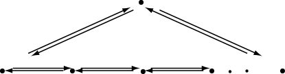
Figure 2: Quiver diagram for the $A_{n-1}$ singularity.

Thus the singularities can be said to be locally quiver. From the point of view of the center of the algebra, the nodes of the quiver are at the same point, but they are distinct in the non-commutative algebra. The behavior of the field theory near the singularities is precisely what we would get from the orbifold analysis.

Recall that the commutative singular lines are covered by $n$ non-commutative branches. The monodromies of the quiver diagram are encoded in this structure, and thus their calculation is geometrically obvious. This compares quite favorably to the rather cumbersome procedure employed in [7]. Indeed, we can change $a\to\omega a$ for $\omega=e^{2\pi i/n}$. This results in a permutation of the factors appearing on the right-hand side of eq. (48). This permutation is the monodromy.

4.2 Adding one mass term

Next, we consider a relevant deformation of the last theory, obtained by the addition of a single mass term. This theory is a $q$-deformed version of the theory which flows in the infrared to an $N=1$ conformal field theory[1, 8]. The superpotential is

$$W={\rm tr}\left(\phi_{1}\phi_{2}\phi_{3}-q\phi_{2}\phi_{1}\phi_{3}+\frac{m}{2}\phi_{3}^{2}\right)$$ (49)

Again, we assume that $q$ is an $n$-th root of unity. The $F$-term constraints are given by

$$\left[\phi_{1},\phi_{2}\right]_{q} = -m\phi_{3}$$ (50)

$$\left[\phi_{2},\phi_{3}\right]_{q} = 0$$ (51)

$$\left[\phi_{3},\phi_{1}\right]_{q} = 0$$ (52)

As in the previous case, we look for the center of the algebra to obtain the commutative manifold. It is easy to see that $z=\phi_{3}^{n}$ is still in the center. We can also show that

$$[\phi_{1}^{n},\phi_{2}] = \phi_{1}^{n}\phi_{2}-q\phi_{1}^{n-1}\phi_{2}\phi_{1}+q\phi_{1}^{n-1}\phi_{2}\phi_{1}-q^{2}\phi_{1}^{n-2}\phi_{2}\phi_{1}^{2}+\dots$$

$$= \phi_{1}^{n-1}(-m\phi_{3})+q\phi_{1}^{n-2}(-m\phi_{3})\phi_{1}+\dots$$

$$= -m\phi_{1}^{n-1}\phi_{3}\sum_{r=0}^{n-1}q^{2r}$$

which vanishes, apart from at the special values $q=\pm 1$. Similarly one proves that $\phi_{2}^{n}$ is central, away from $q=\pm 1$. For now, we will assume that $q^{2}\neq 1$, and return to these cases later. Thus we have at least three central variables $x=\phi_{1}^{n}$, $y=\phi_{2}^{n}$, $z=\phi_{3}^{n}$.

The variable $w$ is modified by the presence of the mass term. Consider the commutator

$$[\phi_{1}\phi_{2}\phi_{3},\phi_{1}] = \phi_{1}\phi_{2}\phi_{3}\phi_{1}-q\phi_{1}\phi_{2}\phi_{1}\phi_{3}+q\phi_{1}\phi_{2}\phi_{1}\phi_{3}-\phi_{1}\phi_{1}\phi_{2}\phi_{3}$$

$$= m\phi_{1}\phi_{3}^{2}$$

This result may be rewritten as a commutator for $q\neq\pm 1$, and thus we see that

$$w=\phi_{1}\phi_{2}\phi_{3}+\frac{m}{1-q^{2}}\phi_{3}^{2}$$ (54)

is central.

The four variables $x,y,z,w$ are related by

$$xyz=-(-w)^{n}-\left(\frac{m}{1-q^{2}}\right)^{n}z^{2}$$ (55)

This is a deformation of the complex structure of (42). It is easy to see that we now have singularities at $w=xz=yz=xy+2tz=0$ with $t=(m/(1-q^{2}))^{n}$. Thus, the singularities are at $xy=0,w=0,z=0$, and so we have two lines of singularities $x=0$ and $y=0$. The mass term has resolved one of the three complex lines of singularities (for $q^{2}\neq 1$).

It is easy to check that a general solution is of the form

$$\phi_{1} = aP$$ (56)

$$\phi_{2} = -bP^{-1}Q-cP^{-1}Q^{-1}$$ (57)

$$\phi_{3} = dQ^{-1}$$ (58)

with $P,Q$ defined as in (45), and where $a,b,c,d$ are numbers satisfying

$$ac(1-q^{2})=md$$ (59)

One then gets $x=a^{n}I$, $y=-(b^{n}+c^{n})I$, $z=d^{n}I$ and $w=-abdI$. Note that this representation has been chosen such that $\phi_{1}$ is diagonal at the singularity $y=0,z=0$.

Because we have a three complex parameter solution of the equations, we at least cover an open patch of the commutative variety, and we are again in a semi-classical ring. Indeed, we cover everything by finite matrices except $x=0$, as then $c$ is infinite.

A patch which does cover $x=0$ is given by

$$\phi_{1} = -aPQ^{-1}-cPQ$$ (60)

$$\phi_{2} = bP^{-1}$$ (61)

$$\phi_{3} = dQ^{-1}$$ (62)

with $ab(1-q^{2})=mqd$. This will be a good description for $y\neq 0$. The two patches cover the two lines of singularities. There is still the closed set $x=y=0$ which is not covered by either patch. We can find solutions for this set by taking $\phi_{3}$ diagonal and making an ansatz for $\phi_{1}$ which is upper triangular with entries just off-diagonal and $\phi_{2}$ a similar lower triangular matrix. The dimension of this representation is also $n$ and depends on one complex parameter, namely the eigenvalues of $\phi_{3}$.

On approaching the singularity $y=z=0$ from the bulk, we again get a split set of irreducible representations as follows:

$$\lim_{b,d\to 0}R(a,b,d)=R(a,0,0)\oplus R(qa,0,0)\oplus\dots$$ (63)

4.2.1 Comments on the Infrared CFT

This case is also very interesting from the field theory perspective because by adding one mass term to a theory with three adjoints, we obtain a nontrivial conformal field theory in the infrared.

On the moduli space, we have the following $U(1)$ symmetries

$$a,b,c \to \lambda\gamma a,\lambda\gamma^{-1}b,\lambda\gamma^{-1}c$$ (64)

$$d \to \lambda^{2}d$$ (65)

where we refer to the parameterization for $x\neq 0$. The transformation given by $\gamma$ is an ordinary $U(1)$, while $\lambda$ is the $U(1)_{R}$ symmetry, that of the superpotential in the infrared. The $R$ charges can be chosen in such a way that the superpotential is invariant at the infrared fixed point. Indeed, one can integrate out $\phi_{3}$ and one finds a theory in the infrared with a quartic superpotential

$$\frac{1}{2m}{\rm tr}(\phi_{1}\phi_{2}-q\phi_{2}\phi_{1})^{2}$$ (66)

This superpotential is a marginal deformation of the infrared theory. Note that we also have, in the infrared, a ${\mathbb{Z}}_{2}$ symmetry $\phi_{1}\leftrightarrow\phi_{2}$ which ensures that the anomalous dimensions of $\phi_{1}$ and $\phi_{2}$ are equal. (In the ultraviolet, this ${\mathbb{Z}}_{2}$ symmetry is absent, as we would also have to simultaneously exchange $q\to q^{-1}$ and rescale $m$.) This symmetry exchanges the two singular complex lines of the commutative moduli space.

4.2.2 Special Cases: $q=\pm 1$

Let us return to discuss the moduli space for the cases $q=\pm 1$ from the algebraic point of view.

For $q=1$, which is the $N=4$ theory with one mass term, the moduli space is the set of solutions to

$$[\phi_{1},\phi_{2}]=-m\phi_{3}$$ (67)

with all other commutators vanishing. For an irreducible representation, $\phi_{3}$ is central and thus a constant. Because the commutator of $\phi_{1},\phi_{2}$ is a constant, we get the Heisenberg algebra, and the only finite dimensional representations are those with $\phi_{3}=0$. Thus the moduli space is a commutative space consisting of the symmetric product of the complex plane, ${\mathbb{C}}^{2}$. Notice that this space is of complex dimension two and not complex dimension three as in the generic case studied above. Indeed, in this case the center of the algebra is generated by $\phi_{3}$. Because $\phi_{3}=0$ on the moduli space, we can actually relax the condition for an element being central: we can take $\phi_{1},\phi_{2}$ as central elements, which makes the moduli space commutative.

Indeed, this is a case where the algebra is not semi-classical. The variety associated to the center is the algebra of ${\mathbb{C}}$. The non-commutative space is ${\mathbb{C}}^{2}$, which projects to the origin of ${\mathbb{C}}$. The two have almost nothing in common.

As far as the commutative variety is concerned, the moduli space is a point. Notice that in this case when we integrate out the field $\phi_{3}$ we get the correct dimension of the moduli space by counting fields. This does not happen for generic $q$.

For $q=-1$, we can find the two dimensional solution

$$\phi_{1}=a\sigma_{1},\phi_{2}=b\sigma_{2},\phi_{3}=0$$ (68)

plus two one-dimensional branches where either $\phi_{1}$ or $\phi_{2}$ is zero.

Here, the center is generated by $\phi_{3}^{2}$. Indeed, it can be shown that these solutions exhaust the list of irreducible representations of the $q=-1$ algebra. This result follows from the fact that $[zx,y]\sim z^{2}$, so a finite dimensional representation must have $z^{2}=0$.

The lesson to be learned from these special examples is that the commutative and non-commutative spaces may contain little or no information about each other when the center of the associated algebra is small. In this case, the full algebra is an infinite dimensional vector space over the center, and by considering only finite dimensional representations, we miss a lot of information.

4.3 One mass term and a linear term

We can easily modify the previously studied cases by adding a linear term to the superpotential

$$W={\rm tr}\left(\phi_{1}\phi_{2}\phi_{3}-q\phi_{2}\phi_{1}\phi_{3}+\frac{m}{2}\phi_{3}^{2}+\zeta_{3}\phi_{3}\right)$$ (69)

Note that by a field redefinition of $\phi_{3}$, this is equivalent to adding a mass term $\frac{\zeta_{3}}{m}(q-1){\rm tr}\phi_{1}\phi_{2}$. We will see that the usual intuition for mass terms fails in this case, namely, that the moduli space is not destroyed by the quadratic terms. On the other hand, if we had added ${\rm tr}\phi_{1}\phi_{2}$ for $q=1$, we would indeed expect the space of vacua to be reduced to a set of points.

It is straightforward to show that $x=\phi_{1}^{n},y=\phi_{2}^{n}$, and $z=\phi_{3}^{n}$ are central, and that

$$w=\phi_{1}\phi_{2}\phi_{3}+\frac{m}{1-q^{2}}\phi_{3}^{2}+\frac{\zeta_{3}}{1-q}\phi_{3}$$ (70)

is also central, provided that $q\neq\pm 1$.

The relation between the central elements is

$$xyz=-(-w)^{n}-\left(\frac{m}{1-q^{2}}\right)^{n}z^{2}+\left(\frac{\zeta_{3}}{q-1}\right)^{n}z$$ (71)

and a generic solution of the equations is provided by

$$\phi_{1} = aP$$ (72)

$$\phi_{2} = -bP^{-1}Q+cP^{-1}-dP^{-1}Q^{-1}$$ (73)

$$\phi_{3} = eQ^{-1}$$ (74)

with $ac(1-q)=-\zeta_{3}$, $ad(1-q^{2})=me$, and $x=a^{n}$, $y=-b^{n}+c^{n}-d^{n}$, $z=e^{n}$, $w=-abe$. The singularities now occur at $z=w=0$ and

$$xy=\left(\frac{\zeta_{3}}{q-1}\right)^{n}$$ (75)

The two complex lines of singularities that met at the origin when $\zeta_{3}=0$ are now replaced by a single ${\mathbb{C}}^{*}$, a cylinder. In the parameterization above, this corresponds to $b,d,e=0$. We see that the non-commutative ${\mathbb{C}}^{*}$ is an $n$-fold cover of the cylinder without branch points, and again the monodromies of the cover are manifest, since we chose $\phi_{1}$ diagonal. This is again a semi-classical ring.

In addition, there are finite dimensional representations which may be thought of as deformations of $SU(2)$ representations. These occur for $x=y=0$ and cover regions not captured by the parameterization above. Some solutions give rise to isolated fractional branes at $x=y=0$. A similar effect occurs in Section 4.5 and we will return to a full discussion there.

The values $q=\pm 1$ are special, as in previous cases, in the sense that singularities occur, and the non-commutative algebra is not semi-classical.

4.4 Three linear terms

Consider the superpotential

$$W={\rm tr}(\phi_{1}\phi_{2}\phi_{3})-q\,{\rm tr}(\phi_{2}\phi_{1}\phi_{3})+\sum_{i}(q-1)\zeta_{i}\,{\rm tr}\phi_{i}.$$ (76)

This case was studied in Ref. [6] using gauge invariant variables. Our conclusions will be consistent with that analysis.

For convenience, we have rescaled the $\zeta$ parameters by a factor of $(q-1)$. The $F$-terms give

$$\left[\phi_{1},\phi_{2}\right]_{q}=(1-q)\zeta_{3},\ \ \ \ \left[\phi_{2},\phi_{3}\right]_{q}=(1-q)\zeta_{1},\ \ \ \ \left[\phi_{3},\phi_{1}\right]_{q}=(1-q)\zeta_{2}$$ (77)

A possible parameterization is

$$\phi_{1}=aP-\frac{\zeta_{3}}{b}Q^{-1}P,\ \ \ \ \phi_{2}=-bP^{-1}Q+\frac{\zeta_{1}}{c}Q,\ \ \ \ \phi_{3}=cQ^{-1}+\frac{\zeta_{2}}{a}P^{-1}$$ (78)

Note that $x_{1}=\phi_{1}^{n}$, $x_{2}=\phi_{2}^{n}$ and $x_{3}=\phi_{3}^{n}$ are central, while the fourth central variable takes the form

$$w=\phi_{1}\phi_{2}\phi_{3}-\zeta_{1}\phi_{1}-q\zeta_{2}\phi_{2}-\zeta_{3}\phi_{3}$$ (79)

In the given basis, we find $x_{1}=a^{n}-(\zeta_{3}/b)^{n}$, $x_{2}=-b^{n}+(\zeta_{1}/c)^{n}$, $x_{3}=c^{n}+(\zeta_{2}/a)^{n}$ and $-w=abc+q\frac{\zeta_{1}\zeta_{2}\zeta_{3}}{abc}$.

These four variables are related on the moduli space by

$$x_{1}x_{2}x_{3}-\sum_{i}\zeta_{i}^{n}x_{i}+2\beta^{n}T_{n}\left(-\frac{w}{2\beta}\right)=0,$$ (80)

where $\beta\equiv(q\zeta_{1}\zeta_{2}\zeta_{3})^{1/2}$ and $T_{n}(x)=\cos(n\cos^{-1}x)$ is the $n$-th Chebyshev polynomial of the first kind.

4.5 Three mass terms

Next, we consider a rank 3 mass term of the form

$$W={\rm tr}(\phi_{1}\phi_{2}\phi_{3})-q\,{\rm tr}(\phi_{2}\phi_{1}\phi_{3})+\frac{1}{2}m\sum_{i}{\rm tr}\phi_{i}^{2}.$$ (81)

This superpotential has a ${\mathbb{Z}}_{2}\times{\mathbb{Z}}_{2}$ symmetry that changes two of the $\phi_{i}\to-\phi_{i}$, and a ${\mathbb{Z}}_{3}$ cyclic symmetry that permutes the $\phi_{i}$. This is the remnant of the $SU(4)_{R}$ symmetry group of the $N=4$ SYM theory. The group generators do not commute with each other, and this symmetry is enhanced to $SU(2)$ when $q=1$. Thus the symmetry is a subgroup of $SU(2)$ which contains a ${\mathbb{Z}}_{2}\times{\mathbb{Z}}_{2}$ and a ${\mathbb{Z}}_{3}$ subgroup. These are the symmetries of the tetrahedron, $\hat{E}_{6}$, and since they arise from the $SU(4)$ R-symmetry they are chiral.

This superpotential yields the $F$-flatness conditions (cyclic on $j$, mod 3)

$$\left[\phi_{j},\phi_{j+1}\right]_{q}=\phi_{j+2},$$ (82)

where we have rescaled the fields in order to eliminate a factor of $m$.

We wish to find representations of this algebra; we will not immediately assume that $q$ is a root of unity. There is a certain class of solutions which may be thought of as deformations of representations of $SL(2,{\mathbb{C}})$.

Note that (for $q\neq 1$) there is a one-dimensional representation

$$\phi_{j}=\frac{1}{1-q}$$ (83)

Higher dimensional representations may always be constructed as $\phi_{i}=\frac{1}{1-q}I$, but this is clearly reducible. An irreducible 2-dimensional representation (for $q\neq-1$) is given by

$$\phi_{j}=\frac{-i}{q+1}\sigma_{j},$$ (84)

where the $\sigma_{j}$ are the Pauli matrices. We can construct higher dimensional irreducible representations by making the following ansatz: we suppose that one of the fields, $\phi_{3}$, is diagonal and traceless, and that the other two fields only have non-zero elements just off the diagonals. (For $q=1$, these reduce to standard $M$-dimensional $SL(2,{\mathbb{C}})$ generators). We have not been able to construct a proof that all such irreps may be obtained this way. These are the representations which respect the discrete chiral symmetry of the system, and are all obtained from the deformation of the representations of $SL(2,{\mathbb{C}})$. The eigenvalues will thus be paired $\pm\alpha_{k}$ and will be the same for all three matrices because the symmetries are respected.

The explicit forms for the representation matrices fall into two classes, with dimensions $M=2p$ and $M=2p+1$, the analogues of half-integer and integer spins.

For $M=2p$, one finds

$$(\phi_{1})_{k\ell} = \delta_{k+1,\ell}a_{k}+\delta_{k-1,\ell}\frac{b_{\ell}}{a_{\ell}},$$ (85)

$$(\phi_{2})_{k\ell} = iq^{k-p}\delta_{k+1,\ell}\,a_{k}-iq^{p-k+1}\delta_{k-1,\ell}\,\frac{b_{\ell}}{a_{\ell}},$$ (86)

$$(\phi_{3})_{k\ell} = i\alpha_{k}\delta_{k\ell}$$ (87)

and we have $b_{p+j}=b_{p-j}$ for $j=1,2,\ldots,p-1$, and $\alpha_{p+n}=-\alpha_{p-n+1}$ for $n=1,2,\ldots,p$.

The $a_{k}$’s may all be set to, say, unity, by $SL(M)$ transformations. The $b_{j}$’s are determined recursively by the formula

$$b_{j}=\frac{-\frac{q}{1+q}\sigma_{2(p-j)}[q]+b_{j-1}\left(1+q^{2(p-j)+3}\right)}{q^{2}\left(1+q^{2(p-j)-1}\right)};\;\;\;b_{0}=0,$$ (88)

for $j=1,2,\ldots,p-1$. The recursion relation is solved by

$$b_{k,p}=\frac{q(q^{4p}-q^{2k})(q^{2k}-1)}{(q^{2}-1)^{2}(q^{2p}+q^{2k-1})(q^{2p}+q^{2k+1})}$$ (89)

and notice that all singularities (poles and zeroes) happen for $q$ a root of unity.

All three matrices have the eigenvalues

$$\pm\alpha_{n}=\pm\frac{1}{q^{p-n}(1+q)}\sigma_{2(p-n)}[q].$$ (90)

for $n=1,2,\ldots,p$.

When $M=2p+1$, we have instead

$$(\phi_{1})_{k\ell} = \delta_{k+1,\ell}\,a_{k}+\delta_{k-1,\ell}\frac{b_{\ell}}{a_{\ell}},$$ (91)

$$(\phi_{2})_{k\ell} = iq^{k-p-1/2}\delta_{k+1,\ell}\,a_{k}-iq^{p-\ell+1/2}\delta_{k-1,\ell}\,\frac{b_{\ell}}{a_{\ell}},$$ (92)

$$(\phi_{3})_{k\ell} = i\alpha_{k}\delta_{k\ell}$$ (93)

where $b_{p+n}=b_{p-n+1}$ and

$$b_{n}=\frac{-q\sigma_{p-n}[q^{2}]+b_{n-1}\left(1+q^{2(p-n+2)}\right)}{q^{2}\left(1+q^{2(p-n)}\right)};\;\;\;b_{0}=0,$$ (94)

for $n=1,2,\ldots,p$. The recursion relation is solved by

$$b_{k,p}=\frac{q(q^{2k}-1)(q^{4p}-q^{2k-2})}{(q^{2}-1)^{2}(q^{2p}+q^{2k-2})(q^{2p}+q^{2k})}$$ (95)

and again we see that all singularities happen for roots of unity. We also have $\alpha_{p+r+1}=-\alpha_{p-r+1}$ for $r=0,1,\ldots,p$ and the eigenvalues of each matrix are in this case

$$0,\,\pm\alpha_{n}=\pm\frac{\sigma_{p-n}[q^{2}]}{q^{(M-2n)/2}}$$ (96)

for $n=1,2,\ldots,p$.

Note that the solutions that we have written here are not $D$-flat. However, by standard theorems, there exists such a solution, which is an $SL(M)$ transformation of the stated solutions. Still, we must be careful in drawing conclusions based on these solutions. In particular, there are apparent singularities at special values of $q$. We will analyze this point further in Section 4.5.2.

4.5.1 Finding more solutions

So far, we have found representations of the algebra which in the limit $q\to 1$ reduce to finite dimensional representations of the $SL(2,{\mathbb{C}})$ algebra. We also noted an additional one-dimensional representation which becomes singular in this limit, and therefore corresponds to a vacuum of the theory, which goes to infinity in the limit. This additional solution is characterized by the property ${\rm tr}\phi_{1}\neq 0$, whereas for all the other solutions ${\rm tr}\phi_{1}=0$.

We should ask if there are more irreducible representations of this algebra, that we have not found above. The answer must be yes, because for $q\to-1$ many of the solutions which correspond to irreducible representations of $SL(2,{\mathbb{C}})$ go away to infinity (the eigenvalues of the matrices are rational functions of $q$ with finite numerator and $q+1$ in the denominator. Thus they are infinitely far away in field space, and do not describe vacua of the theory.)

We can construct additional irreps that do not disappear in the $q\to-1$ limit as follows. The discrete subgroup of $SU(2)$ has a three dimensional representation in terms of Pauli matrices, which suggests the following Ansatz for the representations.

The following satisfy the algebra (82)

$$\phi_{1} = \phi_{1}^{\prime}\otimes(-i\sigma_{1})$$ (97)

$$\phi_{2} = \phi_{2}^{\prime}\otimes(-i\sigma_{2})$$ (98)

$$\phi_{3} = \phi_{3}^{\prime}\otimes(-i\sigma_{3})$$ (99)

if we have

$$\left[\phi_{j}^{\prime},\phi_{j+1}^{\prime}\right]_{-q}=\phi_{j+2}^{\prime}.$$ (100)

Thus, if we know solutions for a given $q$, we generate solutions for $-q$ in this way. These representations are reducible. We will refer to the the irreducible representations obtained in this way as twisted. There are two cases to consider, ‘half integer’ spin and ‘integer spin’ representations.

The integer spin representations have each eigenvalue repeated twice, including zero and are split into two irreducible representations with eigenvalues for $\phi_{3}$ in the succession

$$\pm i\alpha_{1}\to\mp i\alpha_{2}\to\pm i\alpha_{3}\to\dots\to 0\to\dots\to\mp i\alpha_{2}\to\pm i\alpha_{1}$$ (101)

These satisfy ${\rm tr}(\phi_{3})\neq 0$, and ${\rm tr}\phi_{1,2}=0$, as these are off-diagonal. The broken ${\mathbb{Z}}_{2}$ exchanges these two representations. By acting with the ${\mathbb{Z}}_{3}$ symmetry we get a total of six new representations for each even-spin irreducible representation of $SU(2)$.

The ‘half-integer’ cases satisfy ${\rm tr}(\phi_{1,2,3})\neq 0$. One can clearly see a splitting into two irreducible representations, but because there is no eigenvalue $0$, this splitting into two is reducible and in total we get four new representations of the algebra. One of these is a ${\mathbb{Z}}_{3}$ singlet, and the other three form a triplet.

4.5.2 Interpreting the singularities

In this section, we will study properties of representations. In general there are two classes of representations, irreducible and reducible. In the reducible case, there is no mass gap (classically) as some part of the gauge group is unbroken (apart from the decoupled $U(1)$). The case of irreducible representations are potentially more interesting as they confine magnetic degrees of freedom. We will exploit $S$-duality to find dual configurations that are electrically confining. Note that as we have not been able to prove that all irreducible representations are accounted for, we cannot be sure that we see all of the vacua. For the sake of the present argument, we will assume that the classification is complete and try to extract conclusions about the non-perturbative behavior of the theory.

The representations we have found are all matrices which are rational functions of $q$. From the solutions (89),(95), we see that there are poles at roots of unity, $q^{n}=1$.

In the case where we have zeroes and not poles, one observes that as we take the limit to an appropriate root of unity, the matrix decomposes in block-diagonal form. Thus the representation becomes reducible in the limit, and we get various copies of the same type representations (of lower dimension). These singularities are interpreted in the field theory as having enhanced gauge symmetry, because the commutant of the representation is larger. If one pictures the vacua of fixed rank as a covering of the $q$-plane, we have branch points at some roots of unity.

There are other singularities at roots of unity in the denominators of the fields $\phi_{2,3}$. As these are not singularities in the eigenvalues of the matrices, it is not clear that these are singular solutions. This may correspond to an unfortunate choice of basis for the representation.

Considering that the roots of unity are special, in the sense that they are related to orbifolds with discrete torsion which have a very nice semi-classical geometry associated to them, and also considering that in the limit $q\to\pm 1$ an infinite family of solutions to the vacua disappear (in this case there are singularities in the eigenvalues of the matrices), it is plausible that these are actually bona-fide singularities and the vacua go to infinity. As we will see, at these values of $q$, there are moduli spaces of vacua and this is how we interpret the singularities.

Let us begin with a discussion of $q=\pm 1$. First, we know that at $q=1$ all of the states which break the chiral symmetry disappear. Thus we get a jump in the Witten index at this special value. It is also the case that here for some representations one sees no signal of the eigenvalues of the matrices being badly behaved, but it is true that we get poles in the off-diagonal elements.

Let us now discuss $q=-1$, paying particular attention to discrete chiral symmetry breaking. For $U(M)$, $M$ even, the $q$-deformed $SU(2)$ representations move off to infinity at $q=-1$, and thus all the irreducible representations come from the ‘half integer’ twisted case. Thus the Higgs vacua break the ${\mathbb{Z}}_{2}\times{\mathbb{Z}}_{2}$ subgroup completely, and the vacuum has an unbroken ${\mathbb{Z}}_{3}$ subgroup. Each of the four vacua have the ${\mathbb{Z}}_{3}$ embedded differently.

For $U(M)$, $M$ odd, there are irreducible representations of either integer or half-integer twisted type. Thus, some of the Higgs vacua break the group to an unbroken ${\mathbb{Z}}_{3}$ as in the previous case, and some leave an unbroken ${\mathbb{Z}}_{2}$ if they are constructed from the ‘integer spin’ type representations. In addition, the $q$-deformed representations survive for $q\to-1$ but are reducible (the matrix elements $b_{k,p}\to 0$).

Notice that in the previous arguments we have used only the perturbative symmetries of the theory. We believe that the $SL(2,{\mathbb{Z}})$ S-duality of $N=4$ SYM is realized and perhaps enlarged in the present case in some way. We will not address that interesting question here; instead, we confine ourselves to a few remarks based on $SL(2,{\mathbb{Z}})$ alone.

Because of the $SL(2,{\mathbb{Z}})$ symmetry, at the $N=4$ point we can make a map of gauge invariant operators between the different dual theories. Thus we can follow the deformations of the theory for any S-dual configuration of the $N=4$ theory we start with.

Because of the symmetries preserved by the superpotential, changing from one dual picture to another keeps the general form of the Lagrangian invariant. Thus we have a map between couplings $(g,q)\to(g^{\prime},q^{\prime})$, and $m\to m^{\prime}(g,q)$. Because at the roots of unity the theory is special (many vacua collide), the roots of unity must be preserved by the S-duality action on the space of field theories, thus the most general holomorphic transformation that keeps $q=1$ fixed and the structure of the singularities is of the form $q\to q^{\pm 1}$.

Given a vacuum that disappears at a root of unity, let’s say a Higgs vacuum, any of the vacua related to it by S-duality also disappear. For $q=-1$ and $M$ even, the trivial vacuum is $S$-dual to the $q$-deformed Higgs vacuum which moves off to infinity as $q\to-1$, and thus the trivial vacuum is also removed. For $M$ odd, again the trivial vacuum is $S$-dual to the $q$-deformed Higgs vacuum. The latter is reducible, and thus does not appear to have a mass gap; we conclude that the trivial vacuum is not confining. There are still the twisted representations, and thus at $q=-1$, confinement implies (discrete) chiral symmetry breaking.

If $q$ is a more general $n$th root of unity, even though we get poles in the $b_{k,p}$, we have not been able to find any gauge invariant chiral quantity which becomes singular. This suggests that the poles are obtained from a coordinate singularity. In any case, there seems to be an upper bound on the number and dimension of irreducible representations, as each of these general representations seems to decompose into irreducibles of smaller rank. The bound is given in terms of $n$.

Thus as $q$ goes to a root of unity, we can obtain enhanced gauge symmetry. If we do an S-duality transformation and use some more general combination of electric and magnetic condensates, there will still be an upper bound on the dimension of irreducibles and thus no mass gap.

The upper bound on the irreducibles also suggests that one can construct a large center for the algebra. Indeed, one can take the direct sum of all the irreducible representations of the algebra we have constructed. If there are no more irreducible representations, this is a finite dimensional reducible representation, and the subalgebra of the $\phi_{i}$ which is the inverse image of the center of the representation is a large center for the full algebra.

Experience with the example in Section 4.3 suggests that in this case one might actually get a moduli space of vacua. As we have argued that we get a finite number of discrete vacua, let us now show that there is a moduli space for roots of unity $q^{n}=1$ with $n>2$.

We would want the moduli space to be built out of the $P,Q$ matrices in some simple fashion. Let us choose $\phi_{1}$ to be diagonal. Without the mass deformation, the $\phi_{i}$ contain $P,Q,P^{-1}Q^{-1}$. Indeed, one can see that only with the powers $P^{\pm 1}$, $Q^{\pm 1}$ can one get a single factor of $q$ in the commutation relations, and there is a potential to get a cancellation of terms. Thus we take

$$\phi_{1}=a_{1}P+a_{2}P^{-1}$$ (102)

Because of the symmetry between $P,Q$, we also take

$$\phi_{2}=a_{3}Q+a_{4}Q^{-1}$$ (103)

and the $q$ commutation relations are as follows

$$\phi_{1}\phi_{2}-q\phi_{2}\phi_{1}\sim PQ^{-1}+QP^{-1}$$ (104)

so we take

$$\phi_{3}=a_{5}PQ^{-1}+a_{6}QP^{-1}$$ (105)

The parameters are related by

$$a_{1}a_{4}(1-q^{2}) = ma_{5}$$ (106)

$$q^{-1}a_{5}a_{2}(1-q^{2}) = ma_{4}$$ (107)

and thus it follows that

$$a_{5}a_{6}=a_{3}a_{4}=a_{1}a_{2}=\frac{qm^{2}}{(1-q^{2})^{2}}$$ (108)

so apart from factors depending on $m,q$, $a_{2i+1}a_{2i}\sim 1$. This cuts the number of variables from six down to three, and (106) provides one more constraint. Thus we are left with a two parameter solution of the $F$-term constraints. More surprisingly, these also solve the $D$-term constraints. These representations are inequivalent as one can show that the gauge invariant vacuum expectation value ${\rm tr}(\phi_{1}^{n})$ is not independent of the $a_{i}$. For $q=\pm 1$, eq. (108) shows that the $a_{i}$ are singular, and ${\rm tr}(\phi_{1}^{2})$ is singular for $q=-1$, thus this branch of moduli space does not appear at these roots of unity, and one only has isolated vacua.

One can also explicitly show that for $q^{3}=1$, the element $x_{i}=\phi_{i}^{3}+\frac{m^{2}}{q}\phi_{i}$ is central. Thus here one gets a large center, as we have four Casimir operators and one relation. The fourth Casimir is of the form

$$w=A\phi_{1}\phi_{2}\phi_{3}+\alpha_{1}\phi_{1}^{2}+\alpha_{2}\phi_{2}^{2}+\alpha_{3}\phi_{3}^{2}$$ (109)

and it is invariant under the full discrete group of symmetries of the potential. A Casimir of this form exists for all $q$, and when $m=0$ it is the familiar $\phi_{1}\phi_{2}\phi_{3}$; it also reduces to the quadratic Casimir of the $SU(2)$ algebra when $q\to 1$.

The commutative space associated to the algebra is again a deformation of the ${\mathbb{C}}^{3}/{\mathbb{Z}}_{3}\times{\mathbb{Z}}_{3}$ orbifold, and it is three complex dimensional. We have only found a two parameter solution of the equations; we believe that this is because we chose a very special form for the solutions, and not necessarily because the ring fails to be semi-classical.

4.6 The General Superpotential

In this section we will try to make progress towards understanding the general deformation, eqs. (3,4). Solving for the center of the general algebra and also finding the most general finite dimensional irreducible representations of the algebra can be quite difficult. There are some cases which are worth singling out among these, because at least we can find some partial solutions to the moduli space problem. We have also seen that semi-classical rings are better behaved than others, as they lead to nice commutative geometries. Finding all possible semi-classical geometries from our sets of constraints is very important as they might correspond to the behavior of $D$-branes at new dual singularities (not necessarily orbifolds with discrete torsion) which can be connected to $AdS_{5}\times S^{5}$. Of particular importance are configurations with conformal invariance, as they might provide new non-spherical horizons[48, 49]. Our analysis is quite incomplete due to the difficulties of the algebraic program involved, but some general comments will be made here.

As the deformations are taken to zero, the algebra looks like a Poisson algebra if we interpret commutators as Poisson brackets. Because we have three variables, and Poisson manifolds are foliated by symplectic manifolds (which are of even dimension), the symplectic form in the full algebra is degenerate and therefore there is at least one constant of motion. This suggests that there is at least one element of the center which can be easily computed. For the $q$-deformations, the element of the center $w=\phi_{1}\phi_{2}\phi_{3}$ exists for arbitrary values of $q$, which suggests that the element of the center is a polynomial of degree less than or equal to three, depending on the chosen perturbation. For marginal deformations, it is indeed of degree three, as will be shown later; for the deformation by three mass terms it is quadratic (the Casimir of the $SU(2)$ algebra).

Because we have commutators we can think of the algebra as deformation-quantization of the Poisson structure. This suggests that we can standard order operators and establish a correspondence between the full algebra, and the algebra of three commuting variables. In standard constructions, this is given by formal power series expansions in a small parameter $\hbar$. As we have argued before, we want to avoid infinite power series, and rather give an explicit solution which shows that the constraints can be standard ordered in some open set. In order to do this, we separate at each order the polynomials in $\phi_{1},\phi_{2},\phi_{3}$ which can be considered as standard ordered.

A choice of standard ordering is important. If we want to find elements of the center, we need to check that their commutators are zero for all the generators of the algebra. Without standard ordering a given expression, it is very hard to decide if it is zero or not in the algebra.

By using the constraints, an arbitrary polynomial operator ${\cal O}$ can be re-ordered into standard ordered form up to small corrections. We write this as

$${\cal O}={\cal O}_{so}+\hbar{\cal O}^{\prime}$$ (110)

${\cal O}_{so}$ is a linear combination of standard ordered monomials, and it is polynomial in $\hbar$. Similarly, we can expand ${\cal O}^{\prime}\sim a_{i}M^{i}$, where the $a_{i}$ are polynomial in $\hbar$ and the $M^{i}$ are a collection of non-standard ordered monomials. Because of the form of the algebras, the degree of ${\cal O}^{\prime}$ as a polynomial in the variables of the algebra is smaller than or equal to the degree of ${\cal O}$. Taking all the possible non-standard ordered monomials of degree less than or equal to some fixed number $g$, we obtain a matrix equation

$$M^{i}=M^{i}_{so}+\hbar a^{i}_{j}M^{j}$$ (111)

Now $\hbar$ is a small parameter, so the matrix

$$A^{j}_{i}=\delta^{j}_{i}-\hbar a_{i}^{j}$$ (112)

is finite dimensional and invertible. Hence, any non-standard ordered operators may be written as linear combinations of the standard ordered operators, where the coefficients are rational functions in the deformation parameters, the denominators coming from $A^{-1}$.

Since the parameters are complex, more generally we need only worry about the possibility of poles in this construction. At such poles, one of two things can happen. Either the basis for standard ordered polynomials is badly chosen, (e.g., the elements become linearly dependent), or there is a true obstruction to standard ordering independent of the basis. This second possibility can happen, if we take $q=0$ for example.

Thus, in principle we can proceed order-by-order in the degree of polynomials to find central elements. Every element of the algebra can be written in standard ordered form, and as the degree of the element is preserved or lowered by the commutation relations, it is a matter of linear algebra to calculate the elements of a given order which are in the center.

Although the procedure is well-defined, it is not efficient, as we need to calculate the matrix $A$ at each order to resolve this problem. Thus a general solution of how the center depends on the parameters is at best difficult to calculate. Also notice that in the examples we have studied, there is no upper bound in degree for elements of the center.

In some cases, we may find a large center; that is, the center is generated by more than one element of the algebra. If the center is large enough, then we may obtain a semi-classical algebra.

Let us consider the case where the algebra ${\cal A}$ is a finitely generated module over its center, with generators $e_{i}$. We can choose one of the generators to be the identity in the ring, and the others will satisfy a multiplication rule of the type

$$e_{i}\cdot e_{j}=f_{ijk}e_{k}$$ (113)

with $f_{ijk}\in{\cal Z}{\cal A}$. On a given irreducible representation of the algebra, the elements of the center can be treated as numbers, and thus we can argue that we have a family of algebras parametrized by the algebraic variety corresponding to the center of the algebra.

Because of the form of eq. (113), we can see that given a vector in the representation of the algebra, its orbit under the action of the $e_{i}$ is finite dimensional. Thus there is an upper bound on the dimensions of the irreducible representations. We can imagine that this upper bound is realized by the branes living in the bulk, and that any other representation with smaller dimension is a fractional brane of some sort. The finite dimensionality of the irreps suggests that the ring is semi-classical, although we have no proof of this assertion. The semi-classical rings that we have studied all have this property, and this suggests that the two conditions might be equivalent.

Let us now consider a few more examples.

4.6.1 General marginal deformations

As an example of the general difficulties that one faces, let us consider a general marginal deformation of the $N=4$ theory. The superpotential is given by

$$W={\rm tr}\left(\phi_{1}\phi_{2}\phi_{3}-q\phi_{2}\phi_{1}\phi_{3}+\frac{\lambda}{3}\left(\phi_{1}^{3}+\phi_{2}^{3}+\phi_{3}^{3}\right)\right)$$ (114)

and the equations we need to solve for the moduli space are (cyclic)

$$\left[\phi_{j},\phi_{j+1}\right]_{q}=-\lambda\phi_{j+2}^{2}$$ (115)

This algebra is homogeneous, and thus if we were able to find a non-trivial irrep, we could scale it to zero: this implies that the moduli space is connected.

For $\lambda=0$ the element of the center that is always present is $w=\phi_{1}\phi_{2}\phi_{3}$, and this suggests that the element of the center is cubic in general. Indeed, a direct calculation shows that

$$(1-q)\phi_{1}\phi_{2}\phi_{3}-\lambda\phi_{1}^{3}+q\lambda\phi_{2}^{3}-\lambda\phi_{3}^{3}$$ (116)

is central.

Let us first consider one-dimensional irreps. These will satisfy (cyclic)

$$(q-1){\phi_{j}}{\phi_{j+1}}=\lambda\phi_{j+2}^{2}$$ (117)

A non-trivial solution will have the $\phi_{j}$ all non-zero complex numbers. We can easily see that this is only solvable provided that

$$(q-1)^{3}=\lambda^{3}$$ (118)

so $(q-1)/\lambda$ is a cube root of unity. Given $\lambda$ and $q$ satisfying these constraints, one can find solutions to the equations where $\phi_{1}$ and $\phi_{2}$ are equal up to cube roots of unity, and then $\phi_{3}$ is determined from the other two. Thus we get three complex lines meeting at the origin, reminiscent of the moduli space for $q$-deformations. Indeed when $\lambda$ and $q$ are related in this way, there is a linear change of basis of the fields which returns the superpotential to a $q$-deformation. Therefore we have new semi-classical rings, but they are related by a change of basis to the ones we already know.

Another thing that we can do is exploit the ${\mathbb{Z}}_{3}$ symmetry which permutes $\phi_{1},\phi_{2},\phi_{3}$. Set $\phi_{1}=aP$, $\phi_{2}=bQ$, $\phi_{3}=cP^{-1}Q^{-1}$; for the $P,Q$ matrices associated to the cube roots of unity, we also have $\phi_{3}^{2}\sim\phi_{1}\phi_{2}$, so three-dimensional irreps of the algebra may exist.

In this case we want to find solutions to (cyclic on $a,b,c$)

$$ab(q\omega-1)=\omega\lambda c^{2}$$ (119)

with $\omega$ a cube root of unity. One can see that this gives us the constraint

$$(q\omega-1)^{3}=\lambda^{3}$$ (120)

For $\lambda\to 0$ we associate the geometry to ${\mathbb{C}}^{3}/({\mathbb{Z}}_{3}\times{\mathbb{Z}}_{3})$ which happens to be one of the orbifolds one can realize globally on a three-dimensional complex torus.

If for $\lambda\neq 0$ we can find a large center, we might be able to compute the full geometry of moduli space, and treat this solution as a fractional brane. Notice that if this is the case, it does not correspond to a ${\mathbb{C}}^{3}/{\mathbb{Z}}_{n}\times{\mathbb{Z}}_{n}$ singularity, as the fractional branes in that case behave differently. Further exploration of this model will be left for future work[38].

5 $D$-branes in near-horizon geometries

So far, we have mainly discussed moduli spaces of vacua and how to include extended objects in the discussion. The analysis has been done directly in the field theory. Now we will try to understand the background and the moduli space that the $D$-branes realize from the AdS/CFT perspective.

The field theory is understood as being dual to the near-horizon geometry of a brane configuration. Because the moduli space is of the form of a symmetric product (built out of smaller components), one can think of adding these small component $D$-branes as probes in the near horizon geometry and testing how the field theory moduli space is realized on these probes.

We will carefully compare the field theory marginal and relevant deformations to the corresponding deformations of $AdS_{5}\times S^{5}$ geometry. In doing so, we uncover and solve several puzzles. In particular, there are new branches of moduli space in the field theory which open up for arbitrarily small values of $q-1$, as discussed in Section 4.1. Uncovering this structure in the string theory will have several bonuses. This nongeneric branch is realized by wrapping a 5-brane on a 2-torus and using this information, we will argue that the mirror symmetry[7] between deformed 5-spheres and orbifolds can be understood as a standard T-duality operation. The two supergravity descriptions are valid in different areas of parameter space. It also becomes clear in this analysis that there is no sense in which the field theories are dual to supergravity on a space; rather, string theory is absolutely necessary for a consistent duality.

We have seen that the moduli space of vacua has very non-trivial behavior in response to the deformations. In particular, the somewhat artificial separation between the center of the algebra and other elements of the algebra is very subtle in field theory. This will be addressed later and we will find a satisfactory solution. If we look at the same construction from the $AdS_{5}\times S^{5}$, each of these perturbations is in the bulk of the $S^{5}$ geometry, and there is no reason to single out any special elements of the algebra.

5.1 Effects of the Background on $D$-branes

It is important to notice that as seen from the $AdS_{5}\times S^{5}$ perspective when one deforms the theory, the $D$-brane moduli space changes drastically. To first approximation, this is because the added potential localizes the $D$-branes to the ‘fixed planes’ of the deformation. But even for very small deformations $q\sim 1$, we can find rational solutions of $q^{n}=1$ for large $n$, and thus the moduli space has non-generic behavior for a large enough number of branes; indeed, we need $n$ such branes to find extra components of moduli space. These new branches can be seen from (48), and predict that the $D$-branes are going to be uniformly distributed on a circle. We take the eigenvalues of matrices to determine the coordinates of the $D$-branes, as in matrix theory[34].

If the branes are point-like then the open string states stretching between them would be massive and one would not find the new branch in moduli space. However, this is clearly inconsistent with our field theory results, and thus we are motivated to find a satisfactory solution within string theory. Note that these extra components of moduli space do not just appear in the vicinity of the origin; rather, they extend to infinity with the rest of $D$-brane moduli space.

The resolution of these issues bears close resemblance to recent results of Myers[17] concerning the dielectric properties of branes in background fields. Since the deformations of the field theory superpotential correspond to non-zero vevs of fields on the 5-sphere, we do indeed expect these phenomena to occur. Roughly speaking, the $D3$-branes should be thought of as $D5$-branes on ${\mathbb{R}}^{4}\times S^{2}$, where, as we show below, the $S^{2}$ is contained in $S^{5}$. In order to find new branches of the moduli space, we want to argue that there are configurations which support massless open string modes, and topologically this will happen when different spheres intersect each other. Thus their centers can be separated, and we can still have massless string states stretching between them.

Now let us begin by analyzing in some detail the map between superpotential deformations and vevs. This material is of course not new, but is included here for completeness.

The $q-1$ and $m$ deformations correspond to background values for magnetic potentials $F_{(3)}^{RR}$ and $H_{(3)}^{NS}$. The mass deformation is not marginal, and will therefore depend on the radial direction of $AdS_{5}$. The field $\tau=C+ie^{-\phi}$ gives the gauge coupling, and will be kept constant. The field $G_{(3)}=F_{(3)}-\langle\tau\rangle H_{(3)}$ is related directly to the superpotential deformations. The harmonic in the ${\bf 10}$ of $SU(4)$ is a tachyon state in the $AdS$, thus this perturbation blows-up in the infrared. The marginal cubic operators correspond to a harmonic of $G_{(3)}$ in the ${\bf 45}$ of $SU(4)$. In this case, there will be no dependence on the radial direction of $AdS$ as the associated scalar is massless in five dimensions; this fact guarantees that we preserve the conformal group to leading order.

Let us now specialize to the marginal deformations. As explained in Ref. [17], $D3$-branes in the presence of $RR$ background fields pick up a dipole moment for higher brane charge, and become extended in two additional dimensions. The simplest topological shape, and the one with the lowest energy, is a 2-sphere centered at the position of the $D3$-brane. Since we are considering a weakly coupled string theory regime, we should take these to be $D5$-branes[16]. More precisely, the $F_{(3)}$ background is dual to $F_{(7)}$ which couples to a $D5$-brane. $F_{(7)}$ has support on ${\mathbb{R}}^{4}\times D^{3}$, where $D^{3}$ is the 3-disk with $S^{2}$ boundary. The $D3$-branes are extended in the ${\mathbb{R}}^{4}$, which in near-horizon geometry is contained in $AdS_{5}$. We thus write $F_{(7)}=\tilde{F}_{(3)}\wedge dVol_{4}$, and integrating, we can normalize it such that

$$\int_{{\mathbb{R}}^{4}\times D^{3}}F_{(7)}=\int_{D^{3}}\tilde{F}_{(3)}$$ (121)

The 3-disk extends along the radial direction of $AdS_{5}$ plus two directions along the the $S^{5}$. As a result, we can write

$$\tilde{F}_{(3)}=d\rho\wedge\tilde{C}_{(2)}$$ (122)

As such, if the effect were solely due to the dielectric effect it is hard to understand how the $D$-branes can have massless states at different angles along the $S^{5}$, as the stretching happens mostly in the radial direction. The $D3$-brane charge of this 5-brane is obtained from a flux through the 2-sphere, $\frac{1}{2\pi}\int_{S^{2}}F=n$.

As follows from Ref. [5], there will also be a background $H_{(3)}^{NS}$ turned on in the presence of the superpotential deformations. If we expect some energy contribution from the integral of $H_{(3)}^{NS}$ over the disk, then the 2-sphere prefers to be stretched along the 5-sphere, because $H_{(3)}^{NS}$ does not have any component along the $AdS$ directions. In general, then, the radius of the disk $D^{3}$ is oriented partially in the radial direction of $AdS_{5}$ and partially in $S^{5}$, as there are two competing effects deforming the branes.

We want to look for configurations where $D3$-branes are intersecting in the sense of intersections of their $S^{2}$’s. This is where we can expect massless string states, at least topologically. The $H^{NS}$ deformation is the one that gives us the deformation of the $D$-branes in the appropriate direction. We will assume that these configurations are supersymmetric and that probes do not affect the background.

For rational $q$, the moduli space has a scaling direction, which follows from the conformal invariance: in the language of Section 4.1, we have

$$a,b,c\to ta,tb,tc$$ (123)

This is reflected in the near-horizon geometry by the fact that if we move $D3$-branes along the radial direction of $AdS_{5}$, they simply rescale–in particular, if we have intersecting branes, they remain intersecting as we perform this motion.

For relevant deformations, such as a mass term, the $RR$ and $NS$ backgrounds grow as we move in along the $AdS_{5}$, and thus we expect the 2-spheres to grow in size along the 5-sphere as we go to the infrared. As in this case the $H_{(3)}$ fields will also have a radial component, then both types of fields $H_{(3)}$ and $\tilde{F}_{(3)}$ help the 2-sphere to grow along the $S^{5}$ and the radial direction. Eventually, the 2-spheres will be of comparable size to the 5-sphere, and at this point, the notion of point-like $D$-branes loses any meaning. To avoid these issues and for ease of calculation, we will treat only marginal deformations in the following sections.

5.2 Size and Configurations of 5-branes

First, let us find the expected size $r$ of an $S^{2}$ associated with a $D3$-brane. We will assume that this $S^{2}$ is small compared to $R_{5}$, the radius of $S^{5}$, but that it is large enough that we can neglect its self-interaction (from opposite sides of the $S^{2}$). We will show that for small deformations, the size grows linearly with the potential. To this effect, we do a probe calculation. We have a geometry which is almost $AdS_{5}\times S^{5}$ generated by some $D$-branes which are at the origin, and we have a small extra $D$-brane which turns into a sphere on which we are going to do our analysis. Because conformal invariance is preserved by the marginal deformations, there can be no dependence on the $AdS$ radial direction in the physical quantities of interest, apart from setting the scale of the physics. We can therefore work in a local frame and ignore redshift factors, etc.

The DBI action for a $D5$-brane determines the energy

$$E_{DBI}=\frac{\mu_{5}}{g}\int d^{2}\Omega\sqrt{\det(G-B+2\pi\alpha^{\prime}F)}-\mu_{5}\int_{D^{3}}\tilde{F}_{(3)}-\mu_{5}\int(2\pi\alpha^{\prime}F-B)\wedge C_{4}$$ (124)

The metric $G$ scales as $r^{2}$, whereas $F$ behaves as $r^{0}$ (by the flux quantization[50]). By expansion of the DBI part for small $r$, we find an energy of the form

$$E=E(D3)+\frac{\alpha}{g}r^{4}-\beta r^{3}+o(r^{5})$$ (125)

We write

$$\int_{D_{3}}H_{(3)}^{NS}=c_{NS}r^{3}\ \ \ \ \ \ \ \int_{D_{3}}\tilde{F}_{(3)}=c_{R}r^{3}$$ (126)

The field strengths are constant over the disk. We will do the analysis ignoring the five-form field strength. At the end, we will compensate for this omission. The general features of the result should not depend on how far we are from the origin. This is how we can justify this omission.

From the energy (124), we see that the $D3$-brane charge is given by the coupling to $C_{4}$

$$Q_{3} = n-\frac{1}{4\pi^{2}\alpha^{\prime}}\int_{S^{2}}B$$ (127)

$$= n-\frac{c_{NS}}{4\pi^{2}\alpha^{\prime}}r^{3}$$ (128)

The expansion of the energy in powers of $r$ now reads

$$E=\frac{\mu_{3}}{g}\left(Q_{3}-\frac{c_{R}}{4\pi^{2}\alpha^{\prime}}r^{3}+\frac{1}{(4\pi^{2}\alpha^{\prime})^{2}2n}r^{4}+\ldots\right)$$ (129)

where $Q_{3}$ is a constant plus small coorrections in $r^{3}$. The result is minimized at

$$\langle r\rangle\simeq\frac{3}{2}(c_{NS}+gc_{R})(4\pi^{2}\alpha^{\prime})^{2}n$$ (130)

The energy at this radius satisfies

$$E=\frac{\mu_{3}}{g}Q_{3}\left(1+\frac{1}{4Q_{3}}\langle r\rangle^{3}(3c_{NS}-gc_{R})+\ldots\right)$$ (131)

This result is puzzling, since it suggests that $n$ $D3$-branes extend to a single $S^{2}$ of radius proportional to $n$, as opposed to a sphere wrapped $n$ times around the solution for a single brane. This result is wrong from several points of view. First, this solution cannot give enhanced $U(n)$ gauge symmetry, as there are no massless states apparent, and suggests a totally different picture of the moduli space, very different for each value of $n$. We must be more careful in interpreting eq. (131).

We interpret the branes as a black hole in the supergravity which is almost pointlike as far as the $S^{5}$ is concerned. One minimizes the energy (129) and then compares the ratios of energy to $D3$-brane charge of two configurations to determine which may be BPS. In fact, $n$ $D5$-branes wrapping an $S^{2}$ of radius $r$ have lower $E/Q_{3}$ than a single $D5$-brane wrapping an $S^{2}$ of radius $nr$. This indicates that the former configuration has the better chance of being BPS.

The stabilization mechanism which impedes the spheres from shrinking further is that the flux of $F$ is quantized. This mechanism has been found when studying $D$-branes from the boundary state formalism for group manifolds[50], but it is clear that it should be a general phenomenon for $D$-branes in non-trivial $H^{NS}_{(3)}$ backgrounds.

Here we see also that the $RR$ charge for the large sphere is not quantized in general as it gets an anomalous defect proportional to $H^{4}n^{3}$. These can be meta-stable boundary states, and in group manifolds these can be calculated exactly[50], where a similar defect in the brane charge quantization condition occurs. When $H_{NS}=0$ the $D$-brane charge is related to K-theory, and then we expect a quantization condition. This puzzle was recently solved in Ref. [51] where there is a back reaction from the bulk which contributes to the 3-brane charge. Thus, eq. (131) is incomplete as it does not take into account the energy associated to this back reaction. However, the ratio $E/Q_{3}$ on the horizon of the brane probe is exact, being the local tension divided by charge. Here the BPS $D$-branes behave better, as we get an anomalous charge which is proportional to the $D$-brane number.

5.3 Large $n$ branches

We now want to find the new branches of moduli space for $q^{n}=1$, by finding the geometric configuration into which it can be deformed. Because the marginal deformation preserves the conformal group, in the near-horizon geometry, the $H_{(3)}^{NS}$ lies entirely along the 5-sphere, and thus the $D$-brane becomes spherical along 5-sphere directions.

For the $q$-deformation, this means that the $D$-branes grow in size linearly with respect to $q-1$, which is the small parameter. This is the important point of the calculation in the previous section. Consider a configuration of $n$ of these 2-spheres, distributed around a circle in $S^{5}$ so that they touch each other. The value of $n$ is proportional to $(q-1)^{-1}$, in accordance with $q^{n}=1$.

In order for the $D$-branes to touch, we need to know the shape of the 2-spheres well. For $|q|=1$, one finds massless states between 2-spheres which are at the same distance from the origin in $AdS$ space. To see this, we can calculate the masses of the off-diagonal states from the superpotential

$${\rm tr}{\phi_{1}\phi_{2}\phi_{3}}-q{\rm tr}{\phi_{2}\phi_{1}\phi_{3}}$$ (132)

with

$$\phi_{1}=\begin{pmatrix}a&0\\ 0&b\end{pmatrix}$$ (133)

These masses are proportional to $a-qb$ and $b-qa$, and thus in order to have massless states for $|b|=|a|$ we need $|q|=1$.

In order to get the 2-spheres to touch when they are at different radii, the dielectric effect on the $D$-brane has to be included, as it is responsible for extending the $D$-brane in the radial direction. We now want to argue that the $D5$-branes laying flat on the $S^{5}$ actually do touch at another point. The reason why this is important is that moving apart a pair of 2-spheres on $S^{5}$ might make it impossible for them to touch again. Because of the geometric setup, if we consider two $D3$-branes at the same location and we move one with respect to the other in moduli space (of one real dimension on the $S^{5}$), we will get two $2$-spheres. Because the solution of the linearized supergravity equations rotates $H_{(3)}^{NS}$ as we move along this one parameter, the spheres become linked on the $S^{5}$. This is explicitly shown in Figure 3.

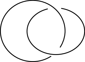
Figure 3: Knotted spheres on $S^{5}$

As the spheres are unlinked when they are very far from each other, they necessarily pass through a point where they touch. This is, topologically, the place where the extra states become massless. With the dielectric effect turned on the spheres are tilted with respect to the $S^{5}$ and that is why they touch at different values of their radial position. The tuning required to make the $D$-branes lie flat on the $S^{5}$ is precisely the action of removing the dielectric effect on the $D$-branes, and corresponds to one real condition on a one complex parameter deformation of the theory.

Thus, we arrive at a configuration of spherical $D5$-branes which touch at points. Now there are configurations, for rational $q$, with $n$ spheres where each touches the next one and they stack on a circle. This is the configuration where the new branch of moduli space opens up, as in eq. (48). This structure should be thought of as a 2-torus with $n$ pinches. Indeed the massless states at the intersection of the $D$-branes are such that they resolve the pinching points into tubes, as in Figure 4.

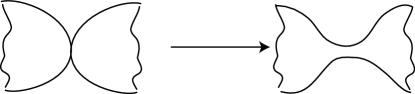
Figure 4: Resolving the pinched Riemann surface

This resolution of these configurations is equivalent to moving onto the new branches of moduli space.

A pinching torus with $n$ nodes is also exactly the degeneration which produces fractional branes in an ALE singularity or on an elliptically fibered Calabi-Yau in F-theory. Thus this configuration of branes seems to be the right one to deform into the extra branches of moduli space for the rational values of $q$.

Notice also that this semi-classical torus is reflected also in equations (45), where we see a realization of a non-commutative torus algebra via clock and shift operators. Thus the non-commutative geometry description of the moduli space knows that the $D$-brane in $AdS_{5}\times S^{5}$ is shaped like a torus, and that when we deform to the degeneration, we split the torus into $n$ spheres (fractional branes), as required by the ALE singularity type of the orbifold in moduli space.

The picture presented above is meant as a topological argument for the branches of moduli space in string theory. These arguments rely upon a few technical assumptions, which we think are reasonable. We have assumed that the different $D$-branes do not affect each other and that they intersect at supersymmetric angles. Although it would be nice to assert this, as it would make our whole construction a purely topological argument, there is no natural complex structure for the spheres which would guarantee this property, and we have to rely on a dynamical mechanism instead. For completeness we should study the possibility that the 2-spheres might interact strongly with each other near the intersection point. In that case, the 2-spheres would develop a throat between them; so, topologically, we have a sphere, with a line bundle of degree two to count the number of D3 branes. When we move in moduli space we deform the line bundle and the metric. For a non-generic bundle, one can get extra states which are massless, and these would be the extra massless modes one needs. Of course, because the field theory tells us that the massless states are there, we believe that these constructions are sensible.

A second point which needs to be made is that although we made an argument based on $D5$-branes, by the $SL(2,{\mathbb{Z}})$ duality we can make an argument with any $(p,q)$-5 brane. Thus the fact that the $RR$ and $NS$ mix in the near-horizon geometry is necessary to implement the $SL(2,{\mathbb{Z}})$ duality on the field theory space of deformations as we change the string coupling $g$ and make different $(p,q)$-strings light. The reason we get a description purely in terms of $D$-branes is that we are using weakly coupled string theory, and for any other brane with $NS5$-brane charge the fundamental strings cannot end on it. This ambiguity in the description has also been found in Ref. [16]. In their case, only one configuration would be such that the supergravity degrees of freedom were weakly coupled through most of the geometry.

5.4 Mirror Symmetry

We have seen that the construction of moduli space suggests a two torus fibration of the five sphere. This torus can be made explicit by using the following invariant coordinates

$$r_{1}^{2}=|\phi_{1}|^{2},r_{2}^{2}=|\phi_{2}|^{2},r_{3}^{2}=|\phi_{3}|^{2},w=\phi_{1}\phi_{2}\phi_{3}$$ (134)

indeed, $\rho^{2}=\sum r_{i}^{2}$ is the radial direction in $AdS_{5}$ and $w$ is equal to $r_{1}r_{2}r_{3}$ except for a phase. We get a total of three real coordinates on the $S^{5}$, and we are left with two phases to determine, which are the arguments of $\phi_{1}/\phi_{2}$ and $\phi_{1}/\phi_{3}$. These two phases determine the two-torus fibration on the $S^{5}$, and the fibration is independent of how many branes are stacked together to get the new branches of moduli space.

Note that the $T^{2}$ so obtained may have $n$ nodes (related to the $D3$-brane charge) but the $T^{2}$ may wrap $m$ times around the $S^{5}$ before closing. The latter clearly corresponds to 5-brane charge. In Ref. [7] a mirror symmetry was noted between string theory on a deformed 5-sphere and an orbifold theory. We are now in position to demonstrate that this mirror symmetry may be obtained by T-duality on the near-horizon geometry, where the T-duality is taken fiberwise on the $T^{2}$ fibration.

The T-duality acts on the 2-torus that we have described above. Explicitly, the charges $(m,n)$ transform as a doublet under the $SL(2,{\mathbb{Z}})$ T-duality. Choose a mapping that takes $(m,n)$, with $m,n$ relatively prime, to $(0,1)$; this mapping will single out a point-like $D3$-brane on the mirror. This is achieved by the matrix

$$M=\begin{pmatrix}a&m\\ b&n\end{pmatrix}$$ (135)

where $a,b$ are fixed numbers, modulo $m,n$ respectively. The torus with complexified Kähler form $K=B+iA$ is taken to a torus with a different value of $K$. Explicitly, we have

$$K\to K^{\prime}=\frac{aK+m}{bK+n}$$ (136)

The area of the torus goes to zero and $B_{NS}$ is smooth at the singularities (where only one phase remains). We can examine the effect of the transformation on $K$ near this limit. Indeed, we get that in the dual torus

$$K^{\prime}\to\frac{m}{n}$$ (137)

which signals a constant $B$-field of strength $m/n$. This value is quantized and its fractional part corresponds to the discrete torsion phase.

As the area of the two torus is not constant, if we start without $H_{NS}$ then upon the T-duality, we will get a varying $B_{NS}$ flux through the dual torus, and thus we have generated an $H_{NS}$ in the T-dual geometry. If we want to cancel this quantity, there is a choice of $B_{NS}$ which makes ${\rm Re}(K^{\prime})=\frac{m}{n}$ constant over the dual fibration. This determines explicitly the $H_{NS}$ field needed to perform the marginal deformation on the field theory, from $q=1$ to a given value of $q$.

Notice that at the singularities we have the allowed degeneration into fractional branes from the splitting of $(m,n)\to n(m/n,1)$. Thus the T-dual fibration has singularities of the $A_{n-1}$ type. As the fractional branes can be connected to each other in moduli space, we get a circle of such singularities and the monodromies around that circle are exactly the ones associated to orbifolds with discrete torsion.

Thus we have both the fractional $B$-field on the T-dual torus, and the monodromies of the singularities so that we can identify the T-dual geometry as the orbifold with discrete torsion.

As we have a T-duality description of the relation between the two compactifications, if the Kähler form is generically large in one setup, it is small in the other. It is therefore necessary to understand which description can be accounted for by supergravity calculations at a given point.

This question can be answered in $AdS_{5}\times S^{5}$. If we want $n$ $D$-branes to become one of these 2-tori, then $q^{n}\sim 1$, and as we saw before $n\sim 1/H$. The calculation of the $D$-brane action was done in string units, thus the $D$-branes are generically of a size commensurate with the string scale.

When we go to the supergravity regime, the string length is related to the supergravity background by the relation

$$l_{s}\sim\frac{1}{\sqrt[4]{gN}}\ l_{p}.$$ (138)

In the configurations that we have discussed, we have $nr\sim R_{5}\sim\sqrt[4]{gN}$ in string units. Now, in order for $\alpha^{\prime}$-corrections to be small, we must have $r\sim H\lesssim\ell_{s}$, which implies

$$n\gtrsim\sqrt[4]{gN}$$ (139)

Thus if we want $n$ relatively small, $AdS_{5}\times S^{5}$ is a poor description of the geometry unless the total number of branes $N$ is such that $\sqrt[4]{gN}<<n$.

Similarly, for the $S^{5}/\Gamma$ to be large, we need a very large number $N$ of $D$ branes. Indeed, the size of $S^{5}/\Gamma$ is of order

$$r\sim l_{p}/n$$ (140)

For the supergravity approximation to be valid here, we should require that twisted sector states are massive; this is the condition $l_{s}<<l_{p}/n$. As a result, the crossover region is at the same place, $n\sim\sqrt[4]{gN}$. Thus, in the orbifold frame, we need to have $N$ large enough so that $l_{p}>nl_{s}$, whereas for the deformed 5-sphere, we needed $N$ small enough so that $nl_{s}>l_{p}$.

For a general $q$-deformation which is not a root of unity, no supergravity description will be good, and one is forced to take into account all of the stringy corrections to the supegravity equations of motion in order to determine the background.

It is also clear that the strength of the perturbation in string units needed to change the value of $q$ at the boundary is related to the number of branes in the configuration. Thus the limit is not uniform in supergravity. In this sense, it is hard to separate vevs from expectation values, as the supergravity boundary conditions are changed drastically when we change the number of branes.

6 Closed Strings and K-theory

So far we have described features of the moduli space of vacua for point-like (in the sense of non-commutative geometry) $D$-branes in deformed geometries. We want now to present a more complete picture of the field theory. This will have two aspects. First, we discuss the chiral ring of the field theory which has a clear interpretation in terms of the supergravity background and we give an interpretation in terms of the algebra itself. The second point that we wish to address is some of the features of extended branes which are accessible by topological considerations. In particular, this involves a somewhat more detailed understanding of K-theory and of discrete anomalies.

6.1 Closed Strings for Near-Horizon Geometry

Next, we will use ideas from the geometry/field theory correspondence to describe the physics of closed strings from the field theory point of view. This closed string theory is to be thought of as the dual string theory to the field theory of some $D$-branes near a singularity. Our aim is to understand the open string – closed string duality a little better, and how one might expect to realize it in the field theory. We have dealt with four-dimensional field theories so far in the classical regime. Our purpose is now to extract a closed string theory out of the quantum dynamics of the field theory.

The near-horizon geometry will have certain boundary conditions which control the superpotential, and some additional set of boundary conditions which specify the vacuum. That is, there are two contributions to the boundary conditions: those that decay sufficiently fast are related to the moduli of the branes, and those that decay more slowly are related to changes in the superpotential. To fully specify the field theory, we need in addition the correlation functions of operators. First, though, we need an identification of those operators.

We take the closed string states to be single trace operators in the field theory. This is in accordance with the AdS/CFT correspondence[2, 3, 4] in that closed string states are gauge invariant operators in the field theory. The idea is to restrict ourselves now to the chiral ring of the field theory for simplicity, and because in all of our analysis we have kept only the parts which are protected by supersymmetry.

Let us assume first that we have a conformal field theory, and that its associated algebra is semi-classical (e.g., orbifolds with discrete torsion). We will exploit the following idea: the vevs of the closed string states (corresponding to states that decay quickly enough at the $AdS$ boundary) are generated by the stack of $D$-branes being at different locations in the moduli space[48]. With the asymptotic values one reconstructs the near-horizon geometry of a set of parallel $D$-branes by summing over holes[53] with given boundary conditions. Thus we can identify different tadpoles of the string states by motion in the moduli space of vacua. The right question to ask is what region of moduli space gives a vev to an operator.

We will combine this knowledge with the identification of the chiral ring for some geometries. Let us review a few results from Ref. [7]. In that paper it was noticed that for orbifolds with discrete torsion, one could see the twisted and untwisted string states in the near-horizon geometry as coming from traces of different chiral operators. We will review the case of the orbifold ${\mathbb{C}}^{3}/{\mathbb{Z}}_{n}\times{\mathbb{Z}}_{n}$ with maximal discrete torsion.

Chiral operators come in two types

$${\cal O}(k_{1},k_{2},k_{3})={\rm tr}(\phi_{1}^{k_{1}}\phi_{2}^{k_{2}}\phi_{3}^{k_{3}})$$ (141)

with $k_{1}=k_{2}=k_{3}\mod(n)$, which are untwisted states, and

$${\cal O}_{j}(k)={\rm tr}\ \phi_{j}^{k}$$ (142)

which are twisted states so long as $k\neq 0\mod(n)$.

The constraint on the $k_{j}$ for untwisted states is familiar from eq. (41). That is, the center of the algebra is associated with the untwisted states. This shows why the center of the algebra is so important to understand the geometry. Namely, the algebraic geometry of the center of the algebra is the geometry that the closed string sector sees. Here again we see that the geometry of the closed strings is commutative, as in Ref. [21]. The non-commutativity of the moduli space appears from the closed string theory point of view because we have twisted sectors.

Notice that in (46) it is clear that it is the fractional branes which give vevs to the twisted sector strings. This is just as it should be, as we always think of coupling twisted sector strings to fractional branes living at the singularities of the classical space. Although we have discussed chiral operators here, it is more generally possible to distinguish twisted and untwisted states. As well, the same statement may be made if we do not have a conformal field theory.

In the case of $AdS_{5}\times S^{5}$, the $F$-term and $D$-term constraints give us a commutative geometry. Thus the center is the whole algebra, and every closed string state is untwisted and lives in the bulk.

We saw in Section 4 that the behavior under mass deformations was special for $q=\pm 1$. From our analysis, we can now see why this is the case. Namely, for $q=\pm 1$, the mass perturbation is untwisted, and therefore affects the bulk of moduli space. For any other rational $q$, the mass perturbation is twisted, and we expect that it will only affect the vicinity of a singularity.

6.2 Chiral ring revisited and Quantum Groups

Let us analyze the chiral ring in more detail. We have already learned that twisted and untwisted states are associated with traces of central (non-central) elements of the algebra, respectively.

States in the chiral ring are made by taking traces of holomorphic elements of the algebra. There are two steps for this construction. First we need a description of the elements of the algebra, and then we need to interpret the properties of the trace.

Any operator (for the deformations we have studied) can always be written in monomial ordered form for a small enough deformation, as we shown in Section 4.6. The difference between two possible orderings is given by $F$-terms and therefore they correspond to derivatives of other fields. In a conformal theory, these would be descendants and not primaries. For the topological chiral ring, we set all $F$-terms to zero, so the operators are identified as traces of elements of the algebra.

Let us consider the case where we have a conformal field theory in the ultraviolet. Because we have an algebra described by quadratic relations, we have a quantum hyperplane geometry[18]. The operators with the same conformal dimension are homogeneous. On every quadratic algebra of the type described, there is an associated quantum group acting on the algebra. The states of the same degree are associated to the representations of this quantum group. This suggests that there might be a relation between operators in the closed string theory and representations of the quantum group. If this is indeed the case, then the fusion rules of the closed string operators will be related to the fusion rules of the representations of the quantum group algebra. This relation would give testable predictions for $3$-point functions in the deformed $AdS_{5}\times S^{5}$ supergravity. Quantum groups have also made an appearance in near-horizon geometry in the work of Ref. [54] in connection with the stringy exclusion principle[55].

We do have to remember that we associate an operator to an element of the algebra, and that it is not the element of the algebra itself which is the gauge invariant operator. The association is by taking

$${\cal O}(a)={\rm tr}(a)$$ (143)

Because of the cyclic property of the trace, we need the following rule

$${\cal O}(ab)={\rm tr}(ab)={\rm tr}(ba)={\cal O}(ba)$$ (144)

thus the map from the algebra to the operators factors through

$${\cal A}\to{\cal A}/[{\cal A},{\cal A}]$$ (145)

as a vector space. It is the class $[a]$ in ${\cal A}/[{\cal A},{\cal A}]$ that matters, and not $a$ itself.

The space

$${\cal A}/[{\cal A},{\cal A}]=HH_{0}({\cal A})$$ (146)

is actually a homology group of the Hochschild complex[56] and suggests that the chiral ring is in general a cohomology group of the non-commutative space (so long as we have some sort of Poincaré duality). Because of our knowledge of Calabi-Yau manifolds, we can think of the chiral ring as a ring of deformations of a non-commutative complex structure, because we have found a relation with homology. Indeed, for a non-compact orbifold space the ring of deformations of the complex structure is infinite-dimensional because of the non-compactness, and it is associated to a cohomology group of the manifold $H^{2,1}(M)$. This suggests that orbifolds with discrete torsion may be better understood as a non-commutative Calabi-Yau space.

6.3 K-theory

Let us now make a few remarks about K-theory. To this effect we will review some of the results of Section 4.

Let us analyze the results of the $q$-deformation for rational $q$. There we found two types of finite dimensional representations: the representation of a non-commutative point associated to the bulk and some other representations which correspond to fractional branes at a singularity.

The set of non-singular points are all connected, and thus each point defines the same K-theory class. On going to the singularity, the points would split as

$$\lim R_{reg}=\oplus_{i}R^{i}_{sing}$$ (147)

where the subscript indicates that the point belongs to the regular part of the variety, or the singular part.

It so happens that the $R^{i}$ are homotopic to each other. That is, they can be deformed continuously into each other. If $q^{n}=1$, then there are $n$ representations on the right hand side of (147). In K-theory we thus have

$$K(R_{reg})=nK(R_{sing})$$ (148)

and the K-theory of points is generated by the K-theory class of a single singular point. Thus $K_{0}^{p}({\cal A})={\mathbb{Z}}$.

If we add one mass deformation, we find two coordinate patches that cover all of the variety except for a single complex line. This complex line is the complex line of singularities that was resolved by the deformation. One can also find solutions that cover this line of singularities. One still has two complex lines of singularities meeting at the origin, and the K-theory of points is still ${\mathbb{Z}}$. In both of these cases the degree of a point is enough to determine its K-theory class.

For the other rings, we find different phenomena. There are isolated points which correspond to fractional branes which cannot be connected to other singular points. For a rank three mass deformation and $q=\pm 1$ or $q$ not a root of unity, the moduli space is completely destroyed and the number of finite dimensional irreducible representations of the algbera is infinite. These are examples of rings which are not semi-classical, and in these cases the K-theory of points consists of an infinite number of copies of ${\mathbb{Z}}$, one for each irreducible representation. In the other cases, for $q$ a root of unity, the number of isolated points is finite.

The reason why the K-theory of points is not preserved under the deformations of the algebra relies on the fact that this is the K-theory appropriate to algebraic geometry, and not real geometry. This stems from the fact that we are restricting ourselves to the moduli spce of vacua, and we are forbidding transitions that go between the different components in moduli space. This is only appropriate if we are studying BPS objects, so this K-theory would serve to count BPS states, and not brane charges.

The full K-theory that we would need to understand brane-charge properly requires the inclusion of anti-holomorphic data and is less refined. This new K-theory would be the algebraic K-theory of the ${\mathbb{C}}^{*}$ algebra associated to the string compactification. That is, the holomorphic K-theory construction gives too many K-theory classes, and does not give classes for the objects which cannot be represented in the holomorphic setting (e.g., odd dimensional $D$-branes).

The second statement that we want to make in K-theory has to do with extended classes. Indeed, based on discrete anomalies, the orbifolds with discrete torsion have a different K-theory than the commutative one [57, 23, 9, 58] associated to the ordinary orbifold. Our K-theory of points reproduces this result. We can also see the anomaly for extended objects.

Consider the orbifold with discrete torsion ${\mathbb{C}}^{3}/{\mathbb{Z}}_{n}\times{\mathbb{Z}}_{n}$, and consider trying to wrap a brane along the singular complex line $x=y=0$. This is a holomorphic subspace of the manifold. For the brane to cover the complex line, we need to have a lift to the non-commutative geometry, but the non-commutative geometry covers the singular complex line by an n-fold cover. Thus if we write a brane solution which would cover the singular complex line only once (which corresponds to a sheaf of rank $1$), this solution would correspond to a fractional brane. The lifting of this solution is obstructed, because if one lifts a point and does an analytic continuation, the brane would be broken in the non-commutative space. Indeed, we need a sheaf of rank $1$ in the non-commutative sense, and this is a sheaf of commutative rank $n$. Thus the brane charge is quantized in units of $n$ larger than in the standard orbifold, just as expected from the discrete anomaly. We believe that the non-commutative analysis makes the calculation of the anomaly more transparent.

As a final point, note that in principle, we have defined a K-theory that is capable of extending to $B^{NS}\neq 0$. As seen from the AdS/CFT, the deformations corresponding to the superpotentials are obtained by addition of antisymmetric tensors to the background. Our results suggest that the K-theory necessary to study these background is the algebraic K-theory of a non-commutative algebra.

7 Conclusions

In this paper, we have studied relevant and marginal deformations of the $N=4$ SYM theory from a non-commutative algebraic point of view. The moduli space looks like a symmetric product of a non-commutative geometry. This is interesting because it implies that $D$-branes may be considered as independent to a certain extent in the weakly coupled regime. This symmetric space captures well the phenomena of $D$-brane fractionation at singularities. Our approach has led us to the beginnings of a new definition of non-commutative algebraic geometry, which is still under investigation. The center of the algebra plays an important role in this construction, and, indeed, in a string theory picture the commutative subalgebra is related to closed strings, while the full non-commutative algebra is needed for open strings. When studied from the AdS/CFT point of view, the field theories that we studied present new dualities between distinct near-horizon geometries. These dualities are realized by T-duality of a 2-torus fibration of the 5-sphere. Different choices of T-duality lead to different dual near-horizon geometries. These results imply that AdS/CFT is inherently a stringy phenomenon, as they exhibit T-dualities which are not symmetries of classical supergravities. In order to understand this duality, we have constructed the $D$-brane configurations which realize the moduli space. We have found that the point-like $D3$-branes of the $AdS_{5}\times S^{5}$ become non-commutative 5-branes wrapping the torus fibration.

The non-commutative geometric framework suggests a natural formulation of K-theory appropriate to holomorphic data, and this is successful in reproducing the physics of discrete anomalies. This suggests that in general backgrounds the K-theory appropriate to $D$-brane charge is that derived from non-commutative algebra.

Our work suggests several avenues for future research. In particular, it would be of interest to understand the general problem of classifying what we have termed semi-classical algebras. A thorough understanding of this problem should provide new backgrounds in which $D$-branes can propagate, and would shed light on the existence of other dualities in near-horizon geometries.

In more generality, one should study the full problem of non-commutative algebraic geometry, including global questions. With a precise notion of gluing and compactness for example, we could entertain the idea of non-commutative Calabi-Yaus and their stringy geometry.

There are also interesting questions concerning non-perturbative effects, which we would need to understand $S$-dualities for example. We also must be concerned about the possibility of non-perturbative effects modifying our results, through, for example, the appearance of multi-trace operators in the superpotential.

For relevant deformations, there will be renormalization group flows which are reflected in near-horizon geometry. It would be of interest to construct these flows for the examples that we have studied, particularly since one expects that stringy corrections become important in the infrared. The study of correlation functions should also be of interest, with a possible connection to the representation theory of quantum groups.

Generalizations of our work to more complicated quivers is possible and will be explored elsewhere.

Acknowledgments: We wish to thank M. Ando, D. Grayson, A. Hashimoto, A. Jevicki, D. Kutasov, J. Maldacena, A. Strominger and C. Vafa for discussions. We are especially indebted to M. Strassler for a critical reading of this paper. DB thanks Harvard University for hospitality. Work supported in part by U.S. Department of Energy, grant DE-FG02-91ER40677 and an Outstanding Junior Investigator Award.

References

- [1] R. G. Leigh and M. J. Strassler, “Exactly marginal operators and duality in four-dimensional N=1 supersymmetric gauge theory,” Nucl. Phys. B447 (1995) 95–136, hep-th/9503121.
- [2] J. Maldacena, “The large-N limit of superconformal field theories and supergravity,” Adv. Theor. Math. Phys. 2 (1998) 231–252, hep-th/9711200.
- [3] E. Witten, “Anti-de Sitter space and holography,” Adv. Theor. Math. Phys. 2 (1998) 253–291, hep-th/9802150.
- [4] S. S. Gubser, I. R. Klebanov, and A. M. Polyakov, “Gauge theory correlators from non-critical string theory,” Phys. Lett. B428 (1998) 105, hep-th/9802109.
- [5] H. J. Kim, L. J. Romans, and P. van Nieuwenhuizen, “The Mass Spectrum Of Chiral N=2 d = 10 Supergravity On ,” Phys. Rev. D32 (1985) 389.
- [6] M. R. Douglas, “D-branes and discrete torsion,” hep-th/9807235.
- [7] D. Berenstein and R. G. Leigh, “Discrete torsion, AdS/CFT and duality,” JHEP 01 (2000) 038, hep-th/0001055.
- [8] P. C. Argyres, K. Intriligator, R. G. Leigh, and M. J. Strassler, “On Inherited Duality in N = 1 d = 4 Supersymmetric Gauge Theories,” hep-th/9910250.
- [9] D. Z. Freedman, S. S. Gubser, K. Pilch, and N. P. Warner, “Renormalization group flows from holography supersymmetry and a c-theorem,” hep-th/9904017.
- [10] L. Girardello, M. Petrini, M. Porrati, and A. Zaffaroni, “Novel local CFT and exact results on perturbations of N = 4 super Yang-Mills from AdS dynamics,” JHEP 12 (1998) 022, hep-th/9810126.
- [11] C. Vafa and E. Witten, “A Strong coupling test of S duality,” Nucl. Phys. B431 (1994) 3–77, hep-th/9408074.
- [12] R. Donagi and E. Witten, “Supersymmetric Yang-Mills Theory And Integrable Systems,” Nucl. Phys. B460 (1996) 299–334, hep-th/9510101.
- [13] M. J. Strassler, “Messages for QCD from the Superworld,” Prog. Theor. Phys. Suppl. 131 (1998) 439, hep-lat/9803009.
- [14] N. Dorey, “An elliptic superpotential for softly broken N = 4 supersymmetric Yang-Mills theory,” JHEP 07 (1999) 021, hep-th/9906011.
- [15] N. Dorey and S. P. Kumar, “Softly-broken N = 4 supersymmetry in the large-N limit,” JHEP 02 (2000) 006, hep-th/0001103.
- [16] J. Polchinski and M. J. Strassler, “The string dual of a confining four-dimensional gauge theory,” hep-th/0003136.
- [17] R. C. Myers, “Dielectric-branes,” JHEP 12 (1999) 022, hep-th/9910053.
- [18] Y. I. Manin, Quantum groups and non-commutative geometry. Université de Montréal Centre de Recherches Mathématiques, Montreal, PQ, 1988.
- [19] A. Klimyk and K. Schmüdgen, Quantum groups and their representations. Springer-Verlag, Berlin, 1997.
- [20] A. Connes, M. R. Douglas, and A. Schwarz, “non-commutative geometry and matrix theory: Compactification on tori,” JHEP 02 (1998) 003, hep-th/9711162.
- [21] N. Seiberg and E. Witten, “String theory and non-commutative geometry,” JHEP 09 (1999) 032, hep-th/9908142.
- [22] R. Minasian and G. Moore, “K-theory and Ramond-Ramond charge,” JHEP 11 (1997) 002, hep-th/9710230.
- [23] E. Witten, “D-branes and K-theory,” JHEP 12 (1998) 019, hep-th/9810188.
- [24] G. Moore and E. Witten, “Self-Duality, Ramond-Ramond Fields, and K-Theory,” hep-th/9912279.
- [25] M. Artin and J. J. Zhang, “non-commutative projective schemes,” Advances in Mathematics 109 (1994), no. 2, 228–287.
- [26] A. L. Rosenberg, non-commutative algebraic geometry and representations of quantized algebras. Kluwer Academic Publishers Group, Dordrecht, 1995.
- [27] M. Kapranov, “non-commutative geometry based on commutator expansions,” math.AG/9802041.
- [28] A. Hashimoto and N. Itzhaki, “Non-commutative Yang-Mills and the AdS/CFT correspondence,” Phys. Lett. B465 (1999) 142, hep-th/9907166.
- [29] J. M. Maldacena and J. G. Russo, “Large N limit of non-commutative gauge theories,” JHEP 09 (1999) 025, hep-th/9908134.
- [30] M. V. Raamsdonk and N. Seiberg, “Comments on non-commutative perturbative dynamics,” hep-th/0002186.
- [31] S. Minwalla, M. V. Raamsdonk, and N. Seiberg, “non-commutative perturbative dynamics,” hep-th/9912072.
- [32] M. R. Gaberdiel, “Lectures on Non-BPS Dirichlet branes,” hep-th/0005029.
- [33] M. A. Luty and I. Washington Taylor, “Varieties of vacua in classical supersymmetric gauge theories,” Phys. Rev. D53 (1996) 3399–3405, hep-th/9506098.
- [34] T. Banks, W. Fischler, S. H. Shenker, and L. Susskind, “M-theory as a matrix model: A conjecture,” Phys. Rev. D55 (1997) 5112–5128, hep-th/9610043.
- [35] J. A. Harvey and G. Moore, “On the algebras of BPS states,” Commun. Math. Phys. 197 (1998) 489, hep-th/9609017.
- [36] M. R. Douglas, “Topics in D-geometry,” Class. Quant. Grav. 17 (2000) 1057, hep-th/9910170.
- [37] A. Connes, non-commutative geometry. Academic Press Inc., San Diego, CA, 1994.
- [38] D. Berenstein, V. Jejjala, and R. G. Leigh. Work in progress.
- [39] R. Hartshorne, Algebraic geometry. Springer-Verlag, New York, 1977. Graduate Texts in Mathematics, No. 52.
- [40] G. Landi, “An introduction to non-commutative spaces and their geometry,” hep-th/9701078.
- [41] R. Dijkgraaf, E. Verlinde, and H. Verlinde, “Matrix string theory,” Nucl. Phys. B500 (1997) 43, hep-th/9703030.
- [42] M. B. Green, J. A. Harvey, and G. Moore, “I-brane inflow and anomalous couplings on D-branes,” Class. Quant. Grav. 14 (1997) 47–52, hep-th/9605033.
- [43] J. Rosenberg, Algebraic -theory and its applications. Springer-Verlag, New York, 1994.
- [44] A. Sen, “Tachyon condensation on the brane antibrane system,” JHEP 08 (1998) 012, hep-th/9805170.
- [45] M. R. Douglas and G. Moore, “D-branes, Quivers, and ALE Instantons,” hep-th/9603167.
- [46] J. Gomis, “D-branes on orbifolds with discrete torsion and topological obstruction,” hep-th/0001200.
- [47] M. R. Douglas and B. Fiol, “D-branes and discrete torsion. II,” hep-th/9903031.
- [48] I. R. Klebanov and E. Witten, “AdS/CFT correspondence and symmetry breaking,” Nucl. Phys. B556 (1999) 89, hep-th/9905104.
- [49] D. R. Morrison and M. R. Plesser, “Non-spherical horizons. I,” Adv. Theor. Math. Phys. 3 (1999) 1, hep-th/9810201.
- [50] C. Bachas, M. Douglas, and C. Schweigert, “Flux stabilization of D-branes,” hep-th/0003037.
- [51] W. Taylor, “D2-branes in B fields,” hep-th/0004141.
- [52] A. Strominger, S.-T. Yau, and E. Zaslow, “Mirror symmetry is T-duality,” Nucl. Phys. B479 (1996) 243–259, hep-th/9606040.
- [53] D. Berenstein and R. G. Leigh, “Superstring perturbation theory and Ramond-Ramond backgrounds,” Phys. Rev. D60 (1999) 106002, hep-th/9904104.
- [54] A. Jevicki and S. Ramgoolam, “Non-commutative gravity from the AdS/CFT correspondence,” JHEP 04 (1999) 032, hep-th/9902059.
- [55] J. Maldacena and A. Strominger, “AdS(3) black holes and a stringy exclusion principle,” JHEP 12 (1998) 005, hep-th/9804085.
- [56] J.-L. Loday, Cyclic homology. Springer-Verlag, Berlin, 1992. Appendix E by María O. Ronco.
- [57] E. Witten, “Baryons and branes in anti de Sitter space,” JHEP 07 (1998) 006, hep-th/9805112.
- [58] A. Kapustin, “D-branes in a topologically nontrivial B-field,” hep-th/9909089.