Singular Cosmological Instantons Made Regular

Abstract

The singularity present in cosmological instantons of the Hawking-Turok type is resolved by a conformal transformation, where the conformal factor has a linear zero of codimension one. We show that if the underlying regular manifold is taken to have the topology of $RP^{4}$, and the conformal factor is taken to be a twisted field so that the zero is enforced, then one obtains a one-parameter family of solutions of the classical field equations, where the minimal action solution has the conformal zero located on a minimal volume noncontractible $RP^{3}$ submanifold. For instantons with two singularities, the corresponding topology is that of a cylinder $S^{3}\times[0,1]$ with $D=4$ analogues of ‘cross-caps’ at each of the endpoints.

I Introduction

Euclidean quantum gravity provides an approach to some of the most fundamental issues in cosmology. One of these is the question of the initial state of the Universe, both for the background geometry and for the fluctuations. Euclidean methods have long been applied to calculations of quantum fluctuations in inflation, and to tunnelling problems in de Sitter space.

A recent development was the observation that a generic theory of scalar matter coupled to gravity allows a one-parameter family of singular but finite action Euclidean instantons which can be used to describe the beginning of inflating open or closed universes[1],[2]. The free parameter in these solutions is just the value of the cosmological density parameter $\Omega$ today.

The singular nature of these instantons is a cause for concern since it is not clear whether the classical field equations are satisfied at the singularity. In references [3] it was argued that the solutions should be regarded as constrained instantons, described by a collective coordinate to be integrated over in the path integral.

In this paper we clarify what the collective coordinate is and how it is to be integrated over. The singularity is resolved by a conformal transformation. The original ‘Einstein frame’ metric equals a regular underlying metric times a conformal factor with a linear zero of codimension one. The regular metric describes an $RP^{4}$ and the conformal factor is taken to be a section of the nontrivial $Z_{2}$ orientation bundle over $RP^{4}$. Because of the nontrivial twist, the action is not guaranteed to be stationary for solutions of the classical differential equations of motion: additional data enters on a nontrivial three manifold upon which the conformal factor vanishes. We draw an analogy with magnetic monopole solutions on $S^{2}$, where one also has a one parameter family of solutions to the classical field equations of varying action. In our case, when we stationarise the action with respect to the free parameter, we find a lowest action classical solution. We extend these considerations to instantons representing the beginning of closed inflationary universes, with topology corresponding to $S^{3}\times[0,1]$ with cross caps at either end.

Allowing the conformal factor to vanish is clearly incompatible with having a a globally Riemannian manifold with positive definite metric. However, there are reasons for believing that in a quantum theory of geometry such behaviour is inevitable. Our best examples of such geometrical theories are string theory, and two plus one dimensional gravity. In the former, if one takes the Lorentzian path integral seriously, it is not possible to have a globally Lorentzian metric on worldsheets with genus not equal to one. There must be singular points at which the determinant of the world-sheet metric vanishes. Likewise, in two plus one dimensional gravity, it has long been argued that one should also take into account vierbeins which have vanishing determinant.

We believe that the interpretation given here resolves some other worries which have been expressed regarding singular instantons. Since the singularity introduces a ‘conformal boundary’, besides apparently violating the intent of the ‘no boundary’ proposal, conformally coupled radiation might be able to enter or leave the spacetime in an arbitrary manner. In our interpretation, where the apparent ‘conformal boundary’ has antipodal points identified, the underlying smooth manifold is compact and there is no boundary. Likewise the concern raised by Vilenkin [4] that a ‘necklace’ of constrained instantons would have arbitrarily negative Euclidean action is also resolved because the number of surfaces on which the constraint enters is determined topologically. For solutions of maximal $O(4)$ symmetry, the number of such surfaces can only be 0, 1 or 2 and we shall discuss the last two cases here. In our construction, ‘necklaces’ do not occur as solutions of the classical field equations.

II Review

The singular instantons described in [1] are O(4) invariant solutions with line element

$$ds^{2}=d\sigma^{2}+b^{2}(\sigma)d\Omega_{3}^{2}$$ (1)

where $d\Omega_{3}^{2}$ is the round three sphere metric. The Euclidean field equations governing the metric and scalar field $\phi$ are

$$b_{,\sigma\sigma}=-\kappa{b\over 3}\left(\phi_{,\sigma}^{2}+V(\phi)\right),\qquad b_{,\sigma}^{2}=\kappa{b^{2}\over 3}\left({1\over 2}\phi_{,\sigma}^{2}-V(\phi)\right)+1,\qquad(\phi_{,\sigma}b^{3})_{,\sigma}=b^{3}V_{,\phi}(\phi).$$ (2)

Here and below we set $\kappa=8\pi G$ where $G$ is Newton’s constant. As long as the potential $V(\phi)$ is not too steep at large $\phi$ there is a one parameter family of finite action solutions in which the scalar field starts at some $\phi_{0}$ and then rolls uphill. The scale factor $b(\sigma)\sim\sigma$ at the regular pole of the instanton, where $\sigma=0$ and $\phi=\phi_{0}$. As $\sigma$ increases, $b(\sigma)$ takes the form of a deformed sine function. As $b$ approaches its second zero, the scalar field’s motion is antidamped and it runs off to infinity. At the singularity $\sigma_{m}$, the scale factor $b$ vanishes as $(\sigma_{m}-\sigma)^{1\over 3}$, and $\phi$ diverges logarithmically, $\phi\approx-\sqrt{2\over 3\kappa}{\rm ln}\left(C(\sigma_{m}-\sigma)\right)$. From this behaviour it follows that $b^{2}e^{\sqrt{2\kappa\over 3}\phi}$ tends to a constant at the singularity. This constant will turn out to be the ‘radius squared’ of the zero conformal factor locus in the regular underlying metric, and will play the role of the collective coordinate mentioned in the Introduction.

The divergence of $\phi$, and of the Ricci scalar for the metric at the singular point $\sigma_{m}$, may seem physically unreasonable, but the finiteness of the action tells us that we should take these singularities seriously since they are not obviously suppressed in the path integral. In fact we shall show that by a suitable change of variables on superspace, the singularity may be removed thus making the action finite term by term. Another possible complaint is that we have no reason to suppose simple behaviour for the potential $V(\phi)$ at field values much greater than the Planck mass. But whilst the singular instanton solutions do probe arbitrarily large values of $\phi$, calculations of observable quantities such as the density perturbations are very insensitive to the precise form of the potential at large $\phi$, precisely because the potential itself (provided it is not very steep) plays very little role in the vicinity of the singularity. In any case, the theory applies virtually unchanged to potentials which are bounded above and therefore never produced super-Planckian energy densities.

A clue to the interpretation of singular instantons is obtained by rewriting the metric in the form $b^{2}(X)(dX^{2}+d\Omega_{3}^{2})$. One sets $dX=d\sigma/b$, thus $X\propto\sigma^{2\over 3}$. From this it follows that as one approaches the singularity, $b^{2}(X)$ vanishes linearly with $X$, so that the singularity is a linear zero of the conformal factor, of codimension one. Solutions with singularities of the same character were discovered in supergravity some time ago. They describe two dimensional ‘tear-drop compactifications’ of ten dimensional supergravity [5]. As noted by those authors, although the relevant manifolds are noncompact, they possess many desirable properties, including a quantised mass spectrum and unbroken supersymmetry to protect against quantum fluctuations. (Incidentally they also have a chiral spectrum of zero modes, and were in some respects the antecedents of the now more popular orbifold compactifications of eleven dimensional supergravity).

The simple nature of the singularity suggests the interpretation we shall explore below, namely that the conformal factor is a field forced to vanish by a topological constraint. We discuss a suitable constraint in the next section.

III Twisted fields

It is a familiar notion that in infinite space, field theories with degenerate vacua possess topologically stable soliton solutions. The condition of finite energy forces the fields to lie in vacuo at infinity. If the map defined by the fields at infinity onto the vacuum manifold is topologically nontrivial, the field is forced to vanish at isolated points, and solitons occur at these points. Solitons like these are in general only strictly stable if space is infinite. But on finite spaces it is still possible to have zeros enforced topologically, and therefore have topologically stable solitons. This occurs if the field configuration is ‘twisted’. This option exists if there are noncontractible loops on the manifold, and if fields can aquire a minus sign as these loops are traversed. In mathematical terminology a twisted field is a section of a nontrivial fibre bundle, requiring more than one coordinate chart for its definition. The simplest case is a scalar field theory on a circle with a $Z_{2}$ internal symmetry $\phi\rightarrow-\phi$. We have two choices of boundary conditions for $\phi$ - periodic or antiperiodic, see Figure (1). Both are equally natural because there is no physical distinction between $+\phi$ and $-\phi$. As the coordinate increases by the length $L$ of the circle, there is no reason to match $\phi$ to $+\phi$ rather than $-\phi$. In the first case, the configuration space is a trivial bundle over $S^{1}$, but in the second it is a nontrivial bundle, and the scalar field aquires a $-1$ as one passes through the single nontrivial coordinate transition. In the path integral there is no reason not to sum over both the twisted and untwisted sectors.

FIG. 1.: Two coordinate patches covering the circle. In the twisted field sector one must reverse the sign of the scalar field when passing between the two coordinate regions on one of the two overlaps (e.g. the one labelled $-$), but not on the other (labelled $+$).

In the twisted sector of a $Z_{2}$ symmetric scalar field theory, the field must vanish somewhere. The interesting case is where the scalar potential yields spontaneous symmetry breaking, for example $V=-m^{2}\phi^{2}+\lambda\phi^{4}$. In this case, at least for large $L$, energetic considerations prefer that the the field be nonzero over most of space. In the twisted sector one must have an odd number of zeros of $\phi$, whereas in the untwisted sector there must be an even number. For finite $L$ the two vacua involved in each case will mix quantum mechanically, with the symmetric state being the ground state. The theory therefore splits into sectors labelled by a $Z_{2}$ topological charge, equal to $(-1)^{N}$ where $N$ is the number of zeros.

To define the action for twisted fields, one must add the contributions from each coordinate patch. Only one of the two transitions between coordinate patches is nontrivial, so one may take the action to be a single integral evaluated in a single patch, running from $0$ to $L$. The only problem is that we have to differentiate the field across the special point $x=0$, identified with $x=L$. The twisted field must undergo a sign change as one crosses this point. The way to differentiate is to note that within a single coordinate patch the derivative is defined as usual as $d\phi/dx=$ Lim$\epsilon\downarrow 0$ $(\phi(x+\epsilon/2)-\phi(x-\epsilon/2))/\epsilon$. But if one differentiates across the singular point, one must include a compensating minus sign, using instead Lim$\epsilon\downarrow 0$ $(\phi(x+\epsilon/2)+\phi(x-\epsilon/2))/\epsilon$. We define the latter as the covariant derivative of the field, $D\phi$. (One could instead insert the minus sign in front of $\phi(x+\epsilon/2)$, which would reverse the sign of $D\phi$. But like $\phi$ itself, $D\phi$ is only defined up to a sign and nothing physical changes if one reverses it.)

The action is then given by

$${\cal S}=\int dx\left[{1\over 2}(D\phi)^{2}+V(\phi)\right].$$ (3)

FIG. 2.: A soliton solution in the twisted sector. The field is shown in each of two coordinate patches. There is a trivial coordinate overlap (+) where the field is identified at $0$ and $L$, and a nontrivial overlap (-) where the field reverses sign. The solution shown is continuous: this requires that one place the transition between the coordinate patches at the zero of the field. However the transition may be placed anywhere, for example at the maximal value of the field. For any location the action is stationary as long as the covariant derivative is continuous (see text).

For example, choosing the singular point to be located at $x_{0}=0$ the action is an integral running from $0$ to $L$. It is varied subject to the boundary constraint that $\phi(0)=\pm\phi(L)$ in the untwisted and twisted cases, obtaining

$${\delta{\cal S}}=\left[\delta\phi{d\phi\over dx}\right]_{0}^{L}+\int_{0}^{L}dx\delta\phi\left[-{d^{2}\phi\over dx^{2}}+V_{,\phi}\right].$$ (4)

The action is stationary under all field variations about a classical solution $\phi_{c}(x)$ if $\phi_{c}(x)$ obeys the classical field equations away from $x=0$ and if ${d\over dx}\phi(0)=\pm{d\over dx}\phi(L)$, which is just the requirement that the covariant derivative be continuous.

For each value of $L$ there is a stationary configuration in the twisted sector. For small $L$ this configuration is just $\phi=0$. This configuration is common to both the twisted and untwisted sectors, but it is only stable in the twisted sector because the destabilising negative mode $\delta\phi=$ constant is disallowed by the twisted boundary conditions.

For larger $L>\pi m^{-1}$ one can easily check that $\phi=0$ is unstable to a twisted negative mode, and the lowest action solution spontaneously breaks the $Z_{2}$, taking the form shown in Figure 2, with a single zero of the scalar field. We shall show that this solution provides a stable twisted classical vacuum. In the gauge where $\phi$ is continuous there is a ‘kink’ $d\phi/dx|^{+}_{-}$ at the zero of $\phi$, which looks like a charged source coupling to $\phi$. But this ‘charge’ is just a reflection of the change of coordinate chart across the zero.

To find the minimum action state it is convenient to label each field configuration by the by the maximal value of $|\phi|$. Without loss of generality we can take this value of $\phi=\phi_{m}$ to be positive. We can also take the sign flip of the field to occur there. Now the field runs from $-\phi_{m}$ to $+\phi_{m}$, as $x$ runs from $0$ to $L$. However note that we cannot (except by working on a larger covering space - see below) construct a globally valid action involving ordinary integrals and derivatives of the fields. We have to proceed by first introducing an ‘internal boundary’ with the field taking the value $\phi_{m}$, and then treat $\phi_{m}$ as a constrained parameter when we vary the action to obtain the field equations.

We start by assuming the field is monotonic. Now we write the action integral as

$$\int_{0}^{L}dx{1\over 2}\left(\phi^{\prime}-\sqrt{2(V(\phi)-V_{m})}\right)^{2}+2\int_{0}^{\phi_{m}}d\phi\sqrt{2\left(V(\phi)-V_{m}\right)}+LV_{m},$$ (5)

where $V_{m}\equiv V(\phi_{m})$. The first term is positive semidefinite. The action is then bounded below by the value of the second two terms, which we may minimise with respect to $\phi_{m}$. For any $\phi_{m}$, the first term is minimised by an appropriate solution of the classical field equations. For the $\phi_{m}$ which minimises the second two terms, the minimum of the first term is zero. Any other field configuration clearly has larger action and therefore the classical solution is absolutely stable.

If we minimise the second two terms we find

$$V_{,\phi}(\phi_{m})\left(2\int_{0}^{\phi_{m}}{d\phi\over\sqrt{2(V(\phi)-V_{m})}}-L\right)=0.$$ (6)

The nontrivial solution is that which occurs when $V_{,\phi}(\phi_{m})$ is not zero. If this solution exists, we can show it is a minimum by changing variables in the integral to $y=\phi/\phi_{m}$ which runs from $0$ to $1$. After absorbing the $\phi_{m}$ in the denominator, the only $\phi_{m}$ dependence is in the quartic (or more generally the non-quadratic terms) of $V$ and $V_{m}$. Hence we see that the first term in (6) is monotonically increasing with $\phi_{m}$. This, with the fact that $V_{,\phi}(\phi_{m})$ is negative, proves that the second two terms in (5) increase away from the stationary point.

The minimum of the the first term in (5) is obtained when the Bogomol’ny equation $\phi^{\prime}=\sqrt{2(V(\phi)-V_{m})}$ holds. By integrating this we obtain a relation between $L$ and $\phi_{m}$. But this is precisely the condition that the bracketed term in (6) vanishes. Thus the solution to the Bogomol’ny equation minimises the action.

We assumed monotonicity above but it is not hard to show that the energy is always greater for non-monotonic configurations. Notice that stability depends on the higher power terms in the potential - a purely quadratic potential does not allow any nontrivial classical solution except $\phi=0$. In the example we have chosen one can perform the integrals as elliptic integrals K and exhibit the ‘critical behaviour’ in $\phi_{m}$ for $L$ just above $\pi m^{-1}$, $\phi_{m}\propto\lambda^{-{1\over 2}}(L-\pi m^{-1})^{1\over 2}$, with action proportional to $-\lambda\phi_{m}^{4}$.

Note that it was useful in this analyis to label field configurations by the maximal field value $\phi_{m}$, separately minimising the action with respect to $\phi_{m}$ on the ‘internal boundary’ and with respect to variations away from the boundary. The Bogomol’ny equation for example explicitly depends on $\phi_{m}$. This is not a procedure one is used to for untwisted fields, because the ground state configuration is trivial and independent of $L$. In contrast the twisted vacuum depends strongly on $L$, even exhibiting a ‘phase transition’ at $L=\pi m^{-1}$.

In the gravitational instanton case we shall adopt a similar strategy, with $\phi_{m}$ replaced by the maximal value of a certain field $n$ which shall be twisted. The size of the instanton, analogous to $L$, will also be integrated over. Hence we find a one parameter family of classical solutions for each value of either the maximal field value or alternatively the size of the instanton. The action is minimised by one particular solution of the classical field equations.

For a twisted scalar field on a circle, we could have represented the problem on the covering space, a circle twice as large, where we used only the odd Fourier modes for the twisted field. In the nonorientable four dimensional example below this option is not available to us, since we wish to consider an action density which is odd under the $Z_{2}$. If we integrated naively on the covering space we would obtain zero. Instead we must include an orientation flip factor in the integral, which effectively reduces it to one over half the covering space.

IV $RP^{4}$

The $Z_{2}$ we discussed in the previous section was a purely internal symmetry. Next we shall identify a similar $Z_{2}$ symmetry acting on the conformal factor and related to orientation reversals for coordinate patches covering a non-orientable manifold. We are interested in viewing the conformal factor as a twisted field. We therefore consider metrics of the form

$$g_{\mu\nu}(x)=\Omega^{2}(x)g_{\mu\nu}^{R}(x)$$ (7)

where $g_{\mu\nu}^{R}(x)$ is a Riemannian (positive definite) metric which shall be regular in the classical solution but the conformal factor $\Omega^{2}(x)$ is allowed to go negative. We shall in what follows refer to geometrical quantities calculated in the metric $g_{\mu\nu}^{R}$ as being in the ‘Riemannian frame’, using terminology analogous to that used in string theory where one considers the ‘string frame’ or ‘Einstein frame’, which are related by a conformal transformation involving the dilaton field.

We consider a theory with a local $Z_{2}$ symmetry, where the $Z_{2}$ involves changing orientation and, in the twisted sector of the theory, reversing the sign of $\Omega^{2}$. With such a local symmetry we can always choose $\Omega^{2}$ to be positive everywhere except at conformal zeros. Therefore we are not considering ‘anti-Euclidean’ or ‘mixed signature’ spacetimes, but we are allowing zeros of the conformal factor to be topologically enforced.

Let us now explain the reason for linking the sign change of $\Omega^{2}$ with orientation reversal. The gravitational/scalar action density (discussed below) involves terms linear in $\Omega^{2}$ and is therefore odd under the $Z_{2}$. The only way to compensate for a sign change $\Omega^{2}\rightarrow-\Omega^{2}$ is to have the the integration measure $d^{4}x$ change sign under the same $Z_{2}$. This means that for the action to be invariant the orientation of the coordinate system must change each time $\Omega^{2}$ changes sign. Twisted fields by definition undergo an odd number of sign changes as one circumnavigates the background space along certain noncontractible paths. If $d^{4}x$ is to do the same, the manifold must be non-orientable, and we must identify the $Z_{2}$ of the twisted line bundle with the $Z_{2}$ of the orientation bundle.

$RP^{4}$ is the obvious candidate manifold, obtained from $S^{4}$ by identifying antipodal points. There is no global choice for orientation on it. The orientation bundle over $RP^{4}$ has a $Z_{2}$ structure group, and we shall identify some scalar fields (including $\Omega^{2}$) as odd and twisted under this $Z_{2}$. We shall obtain an invariant action in the twisted sector, and the singular instantons of Section II will emerge as solutions of the classical field equations in this sector.

FIG. 3.: Three coordinate patches covering $RP^{2}$, forming three of the six faces of a cube and with the identifications indicated by arrows. The boundary of the three patches is an $RP^{1}$ which plays the role of an ‘internal boundary ’ when one constructs the action integral.

The space $RP^{2}$ is easier to visualise than $RP^{4}$ and shares the features of non-orientability, and a class of noncontractible codimension one submanifolds, which shall be central to the discussion below. $RP^{2}$ is illustrated in Figure (3). A sphere may be projectively mapped in a one to one manner onto the surface of a cube. $RP^{2}$ is then formed from three faces of the cube by identifying edges as shown in the diagram on the left in Figure (3). We can further simplify the diagram by mapping the whole onto a disk as on the right of Figure (3). The coordinate patches may be extended into small overlap regions. Each of the three patches connects to the other two via two alternate overlap regions. The first involves crossing the labelled boundary $abc$ and a change in orientation, Jacobian $det(\partial x^{\prime}/\partial x)$ being negative. The other does not, and the Jacobian is positive. (This is made clear by using the obvious Cartesian coordinates on the three faces of the cube). The second important feature is that there is a class of noncontractible $RP^{1}$’s on $RP^{2}$, the most obvious member of which is the $RP^{1}$ boundary $abc$ of the three faces shown in Figure (3) with appropriate identifications. (Note that $RP^{1}$ is isomorphic to $S^{1}$: but the same is not true of $RP^{n}$ for $n>1$). More generally any closed path in $RP^{2}$ which intersects the $RP^{1}$ an odd number of times is noncontractible, and as one travels along it one must pass through an odd number of nontrivial coordinate transitions.

An important check that we have a consistent fibre bundle is that the product of $Z_{2}$ group elements in triple overlap regions, $g_{\alpha\beta}g_{\beta\gamma}g_{\gamma\alpha}$ should be unity. This is indeed satisfied here because in such a triple overlap (shaded region on the right of Figure (3) two of the transitions involve a charge of orientation and the other does not. In the case of $RP^{4}$ the construction is completely analogous except we take half of the faces of a five dimensional hypercube. There is a class of noncontractible $RP^{3}$’s analogous to the $RP^{1}$’s here and as for $RP^{2}$ one can pick one of them to be the one across which the nontrivial field sign and orientation flips occur.

The action for twisted fields takes the form

$$S=\Sigma_{i}\int d^{4}x_{i}\sqrt{g}L_{i}$$ (8)

where the sum runs over coordinate patches, and the integral is broken into non-overlapping pieces with common boundaries within the coordinate overlaps. If the Lagrangian density is a twisted scalar, then moving these boundaries around the manifold does not change the action since the minus sign from the Jacobian $det(\partial x/\partial x^{\prime})$ is compensated for by the minus sign aquired by the Lagrangian density. Note that the determinant $g$, according to the usual transformation laws does not aquire a sign change under an orientation flip and so it is an ‘untwisted’ tensor density.

The action is a functional of the fields in the ‘bulk’ of the $RP^{4}$, with an ‘internal boundary’ which is $RP^{3}$. To write it explicitly we may employ the covering space $S^{4}$, which consists of two identical copies of the $RP^{4}$. Twisted fields are then just odd parity functions on $S^{4}$ while untwisted fields are even parity functions. The two copies of $RP^{4}$ are joined on an even parity three-surface, which consists of two copies of $RP^{3}$. However there is a subtlety associated with integration over the $RP^{4}$. As we have explained, the integral of a twisted scalar is perfectly well defined on $RP^{4}$. But if we use the naive integration measure on $S^{4}$, a twisted scalar would integrate to zero. Instead we must define the integration measure by building in an orientation flip on the three surface common to the $RP^{4}$’s. This involves multiplying $d^{4}x\sqrt{g}$ by a twisted function $\epsilon(x)$ which equals $+1$ on one side and $\epsilon=-1$ on the other side (Figure (4) Now when we integrate a twisted (odd parity) field over the $S^{4}$ and divide by two we get the correct integral over $RP^{4}$. The function $\epsilon(x)$ effectively introduces a boundary into the problem, which is as we have explained an $RP^{3}$ since twisted or untwisted fields must be odd or even parity on it as well. This ‘internal boundary’ we introduce has degrees of freedom associated with its location on the $S^{4}$. It is not the boundary of the manifold however, rather it is the location of the orientation flip which occurs as we circumnavigate $RP^{4}$.

FIG. 4.: The covering space $S^{4}$ for $RP^{4}$ upon which we may construct the action. The twisted fields are odd parity on $S^{4}$ and therefore must possess codimension one zeros. When we integrate a twisted field on $RP^{4}$ we must use the measure $\int d^{4}x\epsilon(x)$ on $S^{4}$ where $\epsilon(x)$ is an odd parity field equal to $+1$ on half of the $S^{4}$. The three manifold upon which $\epsilon$ changes sign is noncontractible on $RP^{4}$, and plays the role of a boundary when constructing the action.

V The Action for Twisted Fields

We are now ready to consider the Einstein-scalar theory discussed in Section II. Our first task is to remove the singularity in the metric to obtain well defined field equations. This is done by changing coordinates on superspace to fields which are regular everywhere. The procedure is familiar in the case of singular spacetime coordinates, for example the usual Schwarzchild coordinates for a black hole. Here, as there, the purpose of the change in coordinates is to enable us to pass through the singularity in an unambiguous way to see what is on the other side.

As mentioned above we consider metrics of the form

$$g_{\mu\nu}(x)=\Omega^{2}(x)g_{\mu\nu}^{R}(x)$$ (9)

where the ‘underlying’ metric $g_{\mu\nu}^{R}$ on a compact four-manifold ${\cal M}$ is assumed positive definite and the conformal factor $\Omega^{2}(x)$ is viewed as a scalar field living on ${\cal M}$ which is allowed to vanish. The metric $g^{R}$ shall be regular in the classical solutions we discuss. Writing the metric this way introduces an obvious local symmetry in our (redundant) description of the theory, namely the conformal symmetry

$$\Omega^{2}(x)\rightarrow\omega^{-2}(x)\Omega^{2}(x),\qquad g_{\mu\nu}^{R}(x)\rightarrow\omega^{2}(x)g_{\mu\nu}^{R}(x),$$ (10)

and we shall adopt this symmetry as fundamental in the construction below.

When we write the action integral for $RP^{4}$ we need to take into account the ‘internal boundary’ mentioned above. We can write the integral over $S^{4}$ with an extra function $\epsilon(x)$ as described, or reduce it to an action over one half of $S^{4}$ with a free boundary. The Euclidean Einstein-scalar action for a manifold with a boundary $B$ is

$${\cal S_{E}}=\int d^{4}x\sqrt{g}\left(-{1\over 2\kappa}R+{1\over 2}(\nabla\phi)^{2}+V(\phi)\right)-{1\over\kappa}\int_{B}\sqrt{h}K$$ (11)

where $h$ is the determinant of the induced three-metric and $K$ the trace of the second fundamental form associated with the boundary. The last boundary term is added to remove second derivatives from the action density so that when we vary the action the field equations follow with no constraint on derivatives of the metric normal to $B$. We proceed from this action, which is valid only for positive definite metrics, by changing coordinates on field space to obtain a new action which will be well defined even when the conformal factor vanishes.

Under the conformal transformation, $g=\Omega^{2}g^{R}$, we find the Ricci scalar $R=\Omega^{-2}R^{R}-6\Omega^{-3}\nabla^{2}\Omega$, $K=\Omega^{-1}K^{R}+3\Omega^{-2}n^{a}\nabla_{a}\Omega$, where $n^{a}$ is the unit outward normal to $B$ and of course $\sqrt{g}=\Omega^{4}\sqrt{g^{R}}$, $\sqrt{h}=\Omega^{3}\sqrt{h^{R}}$. With these substitutions and an integration by parts to remove the second derivatives on $\Omega$ the action (11) becomes

$$\int d^{4}x\sqrt{g^{R}}\left(-{1\over 2\kappa}\Omega^{2}R(g^{R})-{3\over\kappa}\left((\nabla\Omega)^{2}-{\kappa\over 6}\Omega^{2}(\nabla\phi)^{2}\right)+\Omega^{4}V(\phi)\right)$$ (12)

$$-{1\over\kappa}\int_{B}\sqrt{h^{R}}\Omega^{2}K^{R}.$$ (13)

The kinetic terms for the fields $\Omega$ and $\phi$ may be written as $\nabla\phi^{I}\nabla\phi^{J}G_{IJ}$ where the metric on superspace (the space of fields) is the matrix $G_{IJ}(\phi_{K})$. The line element is therefore proportional to $-6d\Omega^{2}+\Omega^{2}d\phi^{2}$. Clearly, $\Omega=0$ is a polar coordinate singularity of the ($\Omega$, $\phi$) coordinate system which may be removed by changing to Cartesian coordinates

$$\Omega_{1}=\Omega{\rm cosh}(\sqrt{\kappa\over 6}\phi)\qquad\Omega_{2}=\Omega{\rm sinh}(\sqrt{\kappa\over 6}\phi),$$ (14)

or light cone coordinates

$$\Omega_{\pm}\equiv\Omega_{1}\pm\Omega_{2}.$$ (15)

The global Lorentzian structure of superspace is illustrated in Figure (5). The singular ‘point’ $\Omega=0$ is now seen to actually be the two lines $\Omega_{+}=0$ and $\Omega_{-}$ =0. We shall be interested in solutions to the field equations which intersect these lines.

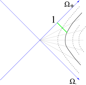
FIG. 5.: The hyperbolic geometry of superspace. The variables $\Omega_{1}$ and $\Omega_{2}$ which are combinations of the scalar field and conformal factor are the natural Cartesian coordinates in which the singularities of singular instantons are resolved. Here light cone axes are plotted, with $\Omega_{\pm}=\Omega_{1}\pm\Omega_{2}$. In the conformal gauge $\Omega_{+}=1$ the solutions start at an arbitrary positive value of $\Omega_{-}$ and ending on one branch of the light cone, $\Omega_{-}=0$, as shown by the line.

In these new regular coordinates the action becomes

$$\int d^{4}x\sqrt{g^{R}}\left(-{1\over 2\kappa}\Omega_{+}\Omega_{-}R(g^{R})-{3\over\kappa}(\nabla\Omega_{+}\nabla\Omega_{-})+(\Omega_{+}\Omega_{-})^{2}V(\sqrt{3\over 2\kappa}{\rm ln}({\Omega_{+}\over\Omega_{-}}))\right)$$ (16)

$$-{1\over\kappa}\int_{B}\sqrt{h^{R}}\left[K^{R}\Omega_{+}\Omega_{-}\right].$$ (17)

This action possesses a lot of symmetry. First, there is general coordinate invariance and conformal invariance of equation (10). Second, there is the $Z_{2}$ symmetry $\Omega^{2}\rightarrow-\Omega^{2}$ and $d^{4}x\rightarrow-d^{4}x$. To implement this symmetry in the regular coordinates we must take one of the light cone coordinates, $\Omega_{-}$ say, to be odd and the other to be even. Note that the potential $V(\phi)$ was only defined for real $\phi$, corresponding to positive $\Omega_{-}/\Omega_{+}$. If we are to define the theory at negative $\Omega_{-}$, we must extend the definition of the potential. The $Z_{2}$ symmetry tells us how to do this, since if the action is to be invariant under the $Z_{2}$, the potential must be an odd function of $\Omega_{-}$. Since what enters the action is $\Omega_{-}^{2}V$, as long as the potential is less divergent than $e^{+2\sqrt{2\kappa\over 3}\phi}$) as $\phi\rightarrow\infty$ then the potential term will tend to zero and be only mildly nonanalytic at $\Omega_{-}=0$.

As we approach a conformal zero, $\Omega^{2}=\Omega_{+}\Omega_{-}$ tends to zero and the potential term becomes negligible. Greater symmetry is then revealed because the kinetic terms in the Lagrangian have an $O(1,1)$ symmetry corresponding Lorentz transformations on superspace, which leave $\Omega^{2}=\Omega_{1}^{2}-\Omega_{2}^{2}=\Omega_{+}\Omega_{-}$ invariant. This symmetry does not commute with the $Z_{2}$ symmetry, and in fact the combined symmetry group is Pin(1,1) [6]. This symmetry is only asymptotically exact as we approach a conformal zero, but if we insist on preserving it we obtain important additional constraints on the action as we now discuss.

As mentioned above, the presence of the orientation flip introduces a boundary into the action being the location of the edge of the coordinate patch with which we attempt to cover the entire $RP^{4}$. The presence of a boundary is an undesirable feature, since a boundary the gravitational action normally allows an arbitrary function of the boundary geometry because the latter is not varied in determining the equations of motion. However the situation we are discussing is much more constrained because of the conformal symmetry of equation (10), and the $O(1,1)$ asymptotic symmetry which we seek to respect. Conformal invariance immediately excludes terms constructed solely from the Riemannian metric $g^{R}$, such as the volume or the integral of the Ricci scalar. If we attempt to include correction factors involving $\Omega_{\pm}$, to restore conformal invariance, the measure term $\sqrt{h^{R}}$ requires odd powers but any curvature invariant requires even powers. Thus we need odd powers of $\Omega_{\pm}$. But these are excluded by $O(1,1)$ symmetry. Thus insisting on the symmetries of the Lagrangian including the asymptotic $O(1,1)$, and insisting the Lagrangian density be regular in the regular coordinates, prohibits any additional boundary contributions to the action apart from an irrelevant constant.

Let us now specialise to $O(4)$ invariant solutions. The Riemannian line element takes the form

$$ds^{2(R)}=N^{2}(\chi)d\chi^{2}+m^{2}(\chi)d\Omega_{3}^{2}$$ (18)

where $N$ is the lapse function. Both $N$ and $m$ are arbitrary functions of $\chi\in[0,\pi)$, which is the polar angle on the covering space $S^{4}$. The metric variables $N$ and $m$ are even parity but $\Omega^{2}$ is odd. It follows that $\Omega^{2}$ must vanish on the equator $\chi={\pi\over 2}$, and that the first derivatives $m^{\prime}(\chi)$ and $N^{\prime}(\chi)$ must vanish there. Since $\Omega_{+}$ is untwisted, and never zero, we may fix the conformal gauge by setting $\Omega_{+}=1$ everywhere. In this gauge we have only one scalar field, namely

$$\Omega_{-}=e^{-\sqrt{2\over 3}\phi}\equiv n,$$ (19)

which by O(4) symmetry and oddness obeys $n=0$ at $\chi={\pi\over 2}$. Finally, when constructing the action on $RP^{4}$ we must include the function $\epsilon(x)$ encoding the orientation reversal, and divide by two. O(4) symmetry forces the sign flip in $\epsilon$ to occur on the equator, so $\epsilon=+1$ for $\chi<{\pi\over 2}$ and $-1$ for $\chi>{\pi\over 2}$. We may of course calculate the action by just integrating over the northern hemisphere. Since $\Omega^{2}$ is zero on the equator, the boundary term in (17) is zero. The boundary conditions at $\chi=0$ are that the Riemannian metric and $n$ should be regular there, so that the field equations are satisfied. This fixes $N^{\prime}(0)=\Omega_{-}^{\prime}(0)=0$, $m(0)=0$ and $m^{\prime}(0)=1$.

In these new variables the usual Einstein-scalar action is

$$2\pi^{2}\int_{0}^{\pi\over 2}d\chi N\left(3\kappa^{-1}(N^{-1}(N^{-1}m^{\prime})^{\prime}m^{2}+N^{-2}{m^{\prime}}^{2}m-m)n+n^{2}m^{3}V(-\sqrt{3\over 2\kappa}{\rm ln}n)\right).$$ (20)

It is useful to leave $N$ in the action so that the Einstein constraint equation emerges by varying with respect to it. But reparametrisation invariance means that all the field equations emerge as equations in the coordinate $\tilde{\chi}=\int_{0}^{\chi}d\chi N$, and henceforth all primes shall denote derivatives with respect to $\tilde{\chi}$. The action may also be written as an integral over $0<\tilde{\chi}<\tilde{\chi}_{max}$, with $\tilde{\chi}_{max}$ being the proper distance in the Riemannian metric from the equator to the north pole. It is the analogue of the length $L$ of the circle in our non-gravitational problem. Because we integrate over the lapse function $N$, $\tilde{\chi}_{max}$ is integrated over in the gravitational path integral.

The action takes the form of that appropriate to a manifold with a boundary, of radius $m(\tilde{\chi}_{max})$, even though as we have emphasised there is really no boundary there. Nevertheless there is a degree of freedom associated with the size of the noncontractible $RP^{3}$ (the singular ‘point’ in the Einstein frame!). We therefore perform the path integral in two steps. For each $RP^{4}$ manifold we find the noncontractible $RP^{3}$ of minimal volume. We then integrate over fluctuations internal to this three surface. Finally we integrate over the geometry of the $RP^{3}$. In the $O(4)$ invariant case, the latter is specified by the radius $m(\tilde{\chi}_{max})$. The action depends on $m(\tilde{\chi}_{max})$ and for generic polynomial potentials has a minimum for one particular value.

The action (20) yields the equations of motion,

$$m^{\prime\prime}n+{1\over 2}m^{\prime}n^{\prime}+{1\over 2}mn^{\prime\prime}=-{\kappa\over 3}V(n)mn^{2},$$ (21)

$$mn^{\prime\prime}+3m^{\prime}n^{\prime}={2\kappa\over 3}mn^{3}{\partial V(n)\over\partial n}$$ (22)

and the constraint which follows from varying with respect to $N$,

$$m^{\prime 2}n+mm^{\prime}n^{\prime}-n=-{\kappa\over 3}V(n)m^{2}n^{2}$$ (23)

where prime denotes derivative with respect to $\tilde{\chi}=\int Nd\chi$. For convenience we henceforth regard the scalar potential $V$ as a function of $n$ which as mentioned above is odd under $n\rightarrow-n$. The equations of motion respect this symmetry. Note that the constraint equation (23) is consistent with the boundary conditions on the equator, namely $n=0$, $m^{\prime}=0$, as long as $n^{2}V$ tends to zero there.

FIG. 6.: The geometry of the solutions for $RP^{4}$, in the Riemannian frame (left) and in the Einstein frame (right).

These field equations are merely a rewriting of those in Section 2, and they possess the same one parameter family of solutions (Figure (6)). The boundary conditions were discussed above - at $\chi=0$ we have $m=0$, $m^{\prime}=1$ and $n^{\prime}=0$, and at $\tilde{\chi}=\tilde{\chi}_{max}$ we have $n=0$ and $m^{\prime}=0$. Both $m$ and $n$ are roughly sinusoidal functions, $m$ starting from 0 at the north pole and increasing towards a final value at the equator, and $n$ decreasing from a constant at $\chi=0$ towards a linear zero on the equator.

A particularly simple case is Garriga’s example based on dimensionally reducing Einstein gravity with a cosmological constant in $D=5$ [8], where $V=\lambda n^{-1}$ with $\lambda$ a constant. The equations of motion have the solutions $m=A^{-1}{\rm sin}A\tilde{\chi}$ and $n=B{\rm cos}A\tilde{\chi}$, with $A=\sqrt{\kappa\lambda/6}$ and $B$ an arbitrary constant. The action (20) is zero for these solutions, as a result of the scale covariance of the theory.

Note that if one worked on the covering space $S^{4}$ and forgot to include the $\epsilon(x)$ correction factor then one would conclude that for any potential there is a one parameter family of regular solutions but with zero action. These solutions would however be half Euclidean and half anti-Euclidean. When one does introduce $\epsilon(x)$, $n$ is replaced by $\epsilon(x)n$ in the action (20). This is even but forced to have zeros at the zeros of $\epsilon$ and $n$, which are both on the equator. The field $\epsilon(x)n$ is positive on both hemispheres but possesses a kink on the equator. Naively, this would mean the equations of motion were violated because the $(\epsilon n)^{\prime\prime}$ terms would introduce a delta function on the equator. But when we vary the action this term arises from the variation with respect to $m$, and on the equator we do not vary $\delta m$. The point is that the minus sign needed in covariant derivatives of twisted fields cannot be incorporated into an action expressible as a single integral covering the whole manifold. Instead we must use a constrained action. This is analogous to the Dirac monopole case we discuss below where the action must be written as the sum of two integrals, and there is a constraint on the boundary where the two integration regions meet. In fact one can see in our case that the classical field equations, (21,22,23) are satisfied for the entire one parameter family of solutions, provided we use covariant derivatives on the twisted field $n$. When we consider $n$ on $RP^{4}$, it has a linear zero on the equatorial $RP^{3}$ and increases in both of the normal directions. However the covariant derivative, as discussed in Section III, involves introducing a relative minus sign in $n$ on either side. Thus the covariant derivative is perfectly continuous in the solutions, and the field equations are satisfied everywhere. Satisfying the classical differential field equations is therefore not sufficient to guarantee a stationary point of the action. In fact the action is different for the one parameter family of classical solutions, but there is a classical solution of minimal action.

We can parametrise the solutions uniquely by the value of the field at the regular pole $\phi_{0}$, or $n_{0}={\rm exp}(-\sqrt{2\kappa\over 3}\phi_{0})$, analogous to the maximum field in Section 3. For gently sloping potentials the equations of motion may be approximately solved [3], yielding

$${\cal S}_{E}\approx-24\pi^{2}M_{Pl}^{4}\left[{1\over V(\phi_{0})}-{\sqrt{3\over 2}M_{Pl}V_{,\phi}(\phi_{0}))\over V^{2}(\phi_{0})}\right]$$ (24)

where $\phi_{0}$ is the initial scalar field value, and $M_{Pl}=\kappa^{-{1\over 2}}$ the reduced Planck mass. The second term is the Gibbons-Hawking surface contribution (in the Einstein frame: as we have mentioned there is no boundary contribution in the Riemannian frame). For simple monomial potentials there is a minimal action solution, typically at a value of $\phi_{0}$ of order $M_{Pl}$.

The minimum of the Euclidean action occurs at the minimal value of $m_{0}=m(\tilde{\chi}_{max})$ for which a classical solution (i.e. a solution of the equations of motion which is regular at the north pole) occurs. To see that a minimum in $m_{0}$ implies an extremum in $S_{E}$, note that both are functions of the maximum $n_{0}$, or the minimal field $\phi_{0}$. But if $m_{0}$ is minimal then $S_{E}$ must be stationary since $(\partial S_{E}/\partial\phi_{0})=(\partial S_{E}/\partial m_{0})(\partial m_{0}/\partial\phi_{0})=0$. (Note that the solutions are labelled uniquely by $n_{0}$ or $\phi_{0}$ but there are two solutions for each $m_{0}$). For the one parameter family of solutions, near the extremum of the action the conformal zero is located on the minimal volume noncontractible $RP^{3}$ in $RP^{4}$ (see Figure (7), and the action $S_{E}$ is minimised. Thus the conformal zero behaves rather like a brane with positive tension. A positive tension brane wrapped around a noncontractible $RP^{3}$ of minimal volume is stable on $RP^{4}$. This leads us to conjecture that the minimal action Euclidean instanton in the above construction is actually stable and has no negative modes [7].

FIG. 7.: The action and other quantities describing the the instanton solution for a simple quadratic potential $V\propto\phi^{2}$. Reduced Planck units are adopted, so that $\kappa=1$. The vertical scale is arbitrary. The action possesses a minimum when the size $m$ of the noncontractible $RP^{3}$ is minimal. The middle graph shows the ‘kink’ in the derivative of the field $n$ on the conformal zero and the lower graph compares the volume of the $RP^{3}$ with that of a three surface stretched over the north pole. As the graph shows, the minimal action instanton occurs when the conformal zero is located on the noncontractible $RP^{3}$ of minimal volume.

It may seem puzzling that an action gives rise to a one parameter family of classical solutions of the field equations when each solution has a different action. The resolution of the paradox is that when the topology is nontrivial the action cannot be expressed as a single global integral but must include constraints present which describe the ‘sewing together’ of the different coordinate charts.

An analogue is provided by the Wu-Yang formulation of the Dirac magnetic monopole on $S^{2}$, which we briefly review. A constant radial magnetic field $\vec{B}=g\vec{r}/r^{3}$ of arbitrary strength solves the field equations $\nabla\times\vec{B}=0$. But the energy functional leading to ths field equation is just the integral over the sphere of ${1\over 2}\vec{B}^{2}$, and is clearly different for all these solutions. The resolution as mentioned is that the action, which is a functional of a gauge non-invariant object, namely the vector potential, is not a single integral but has to be defined over two coordinate patches. If we do attempt to cover the entire $S^{2}$ with a single coordinate patch, we are led to a singular ‘Dirac string’ picture. In the gravitational case above where we attempt to cover $RP^{4}$ with a single coordinate chart we also find a ‘kink’ in the field $n$ leading naively to a delta function in its equation of motion (22).

For the magnetic monopole Wu and Yang explained how to avoid the Dirac string. We describe the monopole in two coordinate patches, covering the upper and lower hemisphere respectively. On the upper hemisphere we set the gauge potential $A_{\phi}=A_{\phi}^{N}=g(1-{\rm cos}(\theta))$ and on the lower hemisphere $A_{\phi}^{S}=g(-1-{\rm cos}(\theta))$. The two are related by a gauge transformation $A_{\phi}^{N}=A_{\phi}^{S}+\partial_{\phi}(2g\phi)$. The total magnetic flux is given by Stokes theorem as $\Phi=\int_{equator}(A_{\phi}^{N}-A_{\phi}^{S})=4g\pi$. When one varies the energy functional $\int^{S}+\int^{N}{1\over 2}\vec{B}^{2}$ with respect to $\vec{A}$, the two surface terms proportional to $\int\delta\vec{A}\times\vec{B}$ are together proportional to the variation in the total magnetic flux. Thus the energy functional is indeed stationary but only when we constrain the total magnetic flux.

In our case the analogue of the flux is the volume of the minimal volume noncontractible $RP^{3}$ on $RP^{4}$. This is a quantity which is invariant under the $Z_{2}$ symmetry and is defined at the coordinate overlap where the $Z_{2}$ symmetry acts, analogous to the magnetic flux above. For Dirac monopoles as is well known the flux is quantised in the presence of electrically charged fields. It is a natural and intriguing question whether there is an analogous quantisation of the volume of the minimal $RP^{3}$. If there were, it would lead to the quantisation of the density parameter $\Omega$ in the Universe.

Finally let us discuss the stability of these solutions under non-$O(4)$-invariant perturbations. We shall only give a heuristic argument in favour of stability. There are two aspects of stability. The first has to do with the location of the conformal zero. As mentioned, this is analogous to a domain wall wrapped on a noncontractible three-cycle of minimal volume, and one could expect the solution to be stable against deformations of the wall location. The second relates to the freedom we had to place the three-surface on which $\epsilon(x)$ switches sign on any even parity three surface (Figure (4) ). It is straightforward to check the solution with least action is the one with the zero of $\Omega_{-}$ located on the three-surface upon which $\epsilon(x)$ flips sign. This is seen by substituting the constraint (23) back into the action (20) and noting that the resulting integrand is proportional to $-6\kappa^{-1}n+2n^{2}V$. For small $n$ the first term dominates and the action density is negative just above the equator, positive below it. The most negative action is therefore obtained by placing the $RP^{3}$ on the equator i.e. the conformal zero, so that the solution has non-negative conformal factor $\Omega^{2}$ in the entire oriented coordinate patch being considered.

VI The Case of Two Singularities

An interesting generalisation of the above construction is obtained by considering the case where the underlying four dimensional manifold is $S^{3}\times[0,1]$, with each end of the resulting cylinder completed by a $D=4$ crosscap. The $D=4$ crosscap can be thought of as either the total space of the twisted line bundle over $RP^{3}$ with fibres trimmed to finite length, or as the space remaining when a single point is removed from $RP^{4}$. Thus the topology we have in mind can be constructed by taking two $RP^{4}$’s, removing a small 4-disk from each and sewing together along the boundaries. The underlying Riemannian manifold is still described by the metric (18) but there is no regular pole, so $m$ is positive everywhere (see Figure (8)). The field $n$ which is $\Omega_{-}$ in the gauge $\Omega_{+}=1$, is twisted and is zero at both the $\tilde{\chi}=0$ and the $\tilde{\chi}=\tilde{\chi}_{max}$ ends. As in the $RP^{4}$ example, the constraints impose $m^{\prime}=0$ on the conformal zeros.

FIG. 8.: The geometry of instantons which are $O(4)$ symmetric and have two singularities in the Einstein frame (right). In the Riemannian frame these singularities are blown up with a conformal transformation into two distinct non-contractible $RP^{3}$’s (left).

The solutions are parametrised by the minimal value of the scalar field $\phi_{0}$, or equivalently the maximum value $n_{0}$, which occurs at the midpoint $\tilde{\chi}=\tilde{\chi}_{max}/2$. Again, with the potential $V=\lambda n^{-1}$, there is a simple family of analytic solutions namely $n=B{\rm sin}\sqrt{2\kappa\lambda/3}\tilde{\chi}$, and $m=\sqrt{3/\kappa\lambda}$. As in the $RP^{4}$ example the action is zero for this special potential because of the scale covariance of the theory.

FIG. 9.: The action and other quantities describing the the instanton solution with two singularities for a simple quadratic potential $V\propto\phi^{2}$. The action possesses a minimum when the size $m_{sing}$ of the $RP^{3}$ on each end is minimal. The middle graph shows the ‘kink’ in the derivative of the field $n$ on the conformal zeros. The lower graph shows the volume of the conformal zero locus in the Riemannian frame (i.e. the two $RP^{3}$’s), $2\pi^{2}m_{sing}^{3}$ (solid line). This may be compared with the volume of the connected three-cycle in the same homology class, obtained by deforming the two disconnected $RP^{3}$’s so that they fuse at the centre, $8\pi\int d\chi m^{2}$. Also shown for comparison is the volume of the equatorial $S^{3}$, $2\pi^{2}m_{reg}^{3}$.

For a quadratic potential $V\propto\phi^{2}$ the action again possesses a minimum, being approximated by the same expression (24) as in the $RP^{4}$ case. The action and other quantities describing the geometry are plotted in Figure (9). We have checked that the ‘radius’ $m$ increases from a minimal value at $\pm\tilde{\chi}_{max}$ to a maximum at the centre $\tilde{\chi}=0$. Thus as in the $RP^{4}$ case the conformal zero is located on the non-contractible three-cycle of minimal Riemannian volume.

VII Singular Instantons and Dimensional Reduction

As demonstrated by Garriga [8], certain $D=4$ singular instanton configurations can be realized as dimensionally reduced nonsingular configurations of $D=5$ pure gravity with a positive cosmological constant $\Lambda$. For concreteness, consider Euclidean gravity on a compact five dimensional manifold $M_{5}$ with action

$${\cal S}=\int_{M_{5}}d^{5}x\sqrt{g_{5}}\left[-\frac{R_{5}}{2\kappa_{5}}+\Lambda_{5}\right]$$ (25)

The desired dimensional reduction to four dimensions amounts to compactifying one dimension of $M_{5}$ on a circle. We write the $D=5$ line element in the form

$$ds_{5}^{2}=\exp\left[\sqrt{\frac{2\kappa_{4}}{3}}\phi\right]ds_{4}^{2}+\exp\left[-2\sqrt{\frac{2\kappa_{4}}{3}}\phi\right]\left(\frac{d\theta}{2\pi}\right)^{2}L^{2}$$ (26)

where $ds_{4}^{2}$ is the four dimensional line element of a metric $g_{4}$ on the dimensionally reduced space $M_{4}$, $\phi$ is a real scalar field, and $\theta\in[0,2\pi)$ is an angular coordinate on a circle of length $L$. The action becomes

$${\cal S}=\int_{M_{4}}d^{4}x\sqrt{g_{4}}\left\{-\frac{R_{4}}{2\kappa_{4}}+\frac{1}{2}(\partial\phi)^{2}+\Lambda_{4}\exp\left[\sqrt{\frac{2\kappa_{4}}{3}}\phi\right]\right\}$$ (27)

where $\kappa_{4}=\kappa_{5}L^{-1}$ and $\Lambda_{4}=\Lambda_{5}L$. Thus, the dimensionally reduced theory looks like gravity on $M_{4}$ plus a minimally coupled scalar field subject to a particular potential. However, if this scheme is to describe a locally non-singular theory in four dimensions, it depends upon the existence of a fibration of $M_{5}$ over $M_{4}$ with $S^{1}$ fibers. Garriga’s observation is that if this topological requirement is relaxed include certain degenerate $S^{1}$ fibrations in which fibers are allowed to shrink to zero size, the result is a class of locally singular $D=4$ configurations which descend from perfectly regular $D=5$ configurations. In the variables of equation (26), these local singularities arise, from the four dimensional viewpoint, as $\phi\rightarrow\infty$ poles, acompanied by conformal zeros in the $D=4$ metric $g_{4}$. These are precisely the Hawking-Turok singular instantons for the case of the simple exponential potential $V(\phi)=\Lambda_{4}\exp\left[\sqrt{\frac{2\kappa_{4}}{3}}\phi\right]$.

Clearly, the five dimensional action of equation (25) has an $O(6)$ symmetric stationary configuration given by the round five sphere of radius $\sqrt{\frac{6}{\kappa_{5}\Lambda_{5}}}=\sqrt{6\over\kappa_{4}\Lambda_{4}}$. However, this solution does not admit a degenerate $S^{1}$ fibration of the type described above. Instead, we pursue an $O(4)\times O(2)$ symmetric ansatz for the metric $g_{5}$ of the form

$$ds_{5}^{2}=\frac{6}{\kappa_{5}\Lambda_{5}}(d\chi^{2}+m(\chi)^{2}d\Omega_{3}^{2}+n(\chi)^{2}d\theta^{2})$$ (28)

where $d\Omega_{3}^{2}$ is locally equivalent to the $O(4)$ symmetric line element on a unit three sphere and $\theta\in[0,2\pi)$ is again an angular coordinate on the unit circle. This metric explicitly describes an $S^{1}$ fibration with degenerate fibers over the locus $n(\chi)=0$. We are led to the $D=5$ stationary configuration given by

$$m(\chi)=\sin(\chi)\text{ \ \ ; \ \ }n(\chi)=\cos(\chi)$$ (29)

with $\chi\in[0,\frac{\pi}{2}]$.

This solution of the $D=5$ field equations looks locally like a five sphere $S^{5}$, but as we discuss below fails globally to give an $S^{5}$ , describing rather the topology of the five-dimensional real projective space $RP^{5}$.

The desired reduction of the five-dimensional stationary configuration of equations (28) and (29) is given by taking

$$\phi\left(\chi\right)=-\sqrt{\frac{3}{2\kappa_{4}}}\log\left({2\pi\over L}\sqrt{\frac{6}{\kappa_{4}\Lambda_{4}}}\cos(\chi)\right)$$ (30)

and

$$ds_{4}^{2}={2\pi\over L}\left(\frac{6}{\kappa_{4}\Lambda_{4}}\right)^{3/2}\cos(\chi)\left(d\chi^{2}+\sin(\chi)^{2}d\Omega_{3}^{2}\right)$$ (31)

which, from the $D=4$ point of view, clearly runs from the regular $\chi=0$ point with $\phi\left(0\right)=-\sqrt{\frac{3}{2\kappa_{4}}}\log\left({2\pi\over L}\sqrt{\frac{6}{\kappa_{4}\Lambda_{4}}}\right)$ to the singular $\chi=\frac{\pi}{2}$ codimension $1$ locus where the metric has a linear conformal zero, and the scalar field $\phi$ rolls off to infinity.

We turn now to an investigation of the global topology of the five dimensional stationary metric given by equations (28) and (29). If this metric is to describe a compact five manifold $N_{5}$, then it gives explicitly a degenerate $S^{1}$ fibration of $N_{5}$ over a four dimensional submanifold $N_{4}$ of $N_{5}$. Furthermore, the $S^{1}$ fibers of this fibration must shrink to zero size precisely over a connected three dimensional submanifold $N_{3}$ of $N_{4}$ with $N_{4}$ and $N_{3}$ locally isometric to the round $S^{4}$ and $S^{3}$, respectively. The $\chi\in[0,\frac{\pi}{2})$ subspace of $N_{5}$ which is the complement $(N_{5}-N_{3})$ is connected. This implies via the degenerate fibration that $(N_{4}-N_{3})$ is connected. Thus it is clear that our five dimensional metric cannot describe a topological $S^{5}$, since this would imply that $N_{4}\cong S^{4}$ and there can be no $N_{3}$ for which $(S^{4}-N_{3})$ is connected. On the other hand, the identifications $N_{5}\cong RP^{5}$, $N_{4}\cong RP^{4}$ and $N_{3}\cong RP^{3}$ do work, since $RP^{n}\cong S^{n}/Z_{2}$ and $(RP^{n}-RP^{n-1})$ can be connected.

This is, in fact, the only possibility and the global topology of the stationary five metric is that of $RP^{5}$, which has a degenerate $S^{1}$ fibration over $RP^{4}$, with ‘zero size’ fibers over a non-contractible $RP^{3}\subset RP^{4}$. This makes explicit the connection with our earlier analysis of Hawking-Turok singular instantons arising as conformal zeros of four metrics wrapped on non-contractible cycles of $RP^{4}$.

We can directly construct this degenerate fibration using homogeneous coordinates on $RP^{5}$

$$(u_{0},u_{1},U)\sim\lambda(u_{0},u_{1},U),\forall\lambda\in(R-{0})$$ (32)

where $u_{0},u_{1}\in R$ and $U\in R^{4}$. The appropriate polar geodesic coordinate $\chi\in[0,\frac{\pi}{2}]$ is given by

$$\tan{\chi}=|U/u_{0}|$$ (33)

For $\chi\in[0,\frac{\pi}{2})$ we can use the scaling freedom of equation (32) to put the $RP^{5}$ coordinates in the form

$$(\xi cos{\chi},Wsin{\chi})$$ (34)

where $\xi=u_{1}/u_{0}$ can be viewed as a local coordinate on $RP^{1}\cong S^{1}$ and $W$ is a point on the unit $S^{3}$. The $RP^{4}$ base for the degenerate fibration can then be defined in homogeneous coordinates by $u_{1}=0$ which amounts to $\xi=0$ in the $\chi\in[0,\frac{\pi}{2})$ subspace of $RP^{5}$. It only remains to identify the submanifold of the $RP^{4}$ over which the fibres go to zero size. This is the $\chi=\frac{\pi}{2}$ subspace which is the $RP^{3}\subset RP^{5}$ defined by $u_{0}=u_{1}=0$. Clearly, the $\chi$ of equation (34) can be identified with the $\chi$ of the stationary five metric given by equations (28) and (29).

So Garriga’s degenerate dimensional reduction emerges as a special case of our realization of a large class of singular instanton configurations via conformal zeros in the four metric of Euclidean spacetime. As in our case, projective manifolds are involved. But there are several ways in which we expect our intrinsically four dimensional analysis to be more fundamental than an analysis of apparently singular dimensional reductions of non-singular $D=5$ gravitational configurations. Firstly, it is not clear why one should insist upon starting from $D=5$. One would expect to reach distinct and apparently singular $D=4$ configurations arising from the reduction of theories in any $D>4$. Is the path integral to sum over configurations in all such higher dimensions? The intrinsic realization of singular stationary points in $D=4$ should arise in a purely four dimensional path integral formulation. The fact that certain of these configurations can be embedded in higher dimensional theories may be useful but is unlikely to be fundamental. Secondly for four dimensional topologies more complicated than $S^{4}$ or $RP^{4}$, we expect Hawking-Turok type singular instantons to arise for four dimensional conformal zeros wrapped around each distinct codimension one integral homology cycle. It is difficult to see how these configurations can be easily accommodated in the degenerate dimensional reduction picture.

As a final remark, let us comment on an apparent discrepancy between the four dimensional theory we have defined, which has zero action for Garriga’s potential, and the five dimensional $RP^{5}$ theory discussed above which has a negative action corresponding to that for a five sphere. The resolution is that in the five dimensional interpretation the boundary condition imposed by regularity at $\chi={\pi\over 2}$ is that $n^{\prime}=1$ so that the singular pole is regular in five dimensions. In our four dimensional picture, however, the boundary condition is that the Riemannian metric radius $m$ should be fixed. The actions appropriate to the two different boundary conditions differ by a term which, as noted by Garriga, is minus two thirds of the usual boundary term given in (11). This explains the discrepancy between the two actions. The four dimensional action and boundary condition we have used also respects the scale covariance $n\rightarrow\lambda n$ of the theory, which as we have mentioned explains why we obtain zero action. The five dimensional boundary condition violates the scale invariance and that is why one obtains a nonzero action.

VIII Conclusion

We have discussed an interpretation of instantons possessing conformal zeros which links those zeros to the topological properties of an underlying Riemannian manifold. One of the interesting points to emerge is that the topologically twisted conformal factor does not admit a description via a globally defined action. We have to use a constrained action in which additional data is defined on an ‘internal boundary’. The classical differential equations of motion are a necessary but not sufficient condition for the stationarity of the resulting action, and we have shown that the one parameter family of singular instanton solutions discussed in Section 2 all satisfy the equations of motion but have differing action. We have shown that in the least action solution, the conformal zero is located on the minimal volume noncontractible $RP^{3}$ submanifold, and therefore behaves somewhat like a brane of positive tension. We generalised these arguments to singular instanton solutions with two singularities which are each resolved in the Riemannian frame into ‘cross-caps’possessing noncontractible $RP^{3}$ conformal zeros. We have provided a regular setting for singular instantons which suggests that they may be stable and possess no negative modes. This is an important difference with the usual Coleman-de Luccia instantons [9].

We have discussed singular instantons with one codimension one conformal zero, which analytically continue to open inflationary Universes. We have also discussed instantons with two codimension one conformal zeros, which analytically continue to closed inflationary Universes. Examples of potentials which give realistic such Universes will be given in a future publication.

Finally, we wish to stress that the idea of allowing conformal zeros is more general and far reaching than the solutions we have explored here. It is a first step towards discussing signature change and topology change in four dimensional quantum geometry. In a forthcoming paper we extend the discussion to higher codimension [6].

This work was supported by a PPARC (UK) rolling grant and a PPARC studentship. We thank M. Bucher, S. Gratton, S.W. Hawking and V. Rubakov for helpful comments on this work.

REFERENCES

- [1] S.W. Hawking and N. Turok, Phys. Lett. B425, 25 (1998).
- [2] R. Bousso and A.D. Linde, Phys.Rev. D58, 083503 (1998).
- [3] N. Turok and S.W. Hawking, Phys. Lett. B432 271 (1998); N. Turok, Phys.Lett. B458 (1999) 202.
- [4] A. Vilenkin, gr-qc/9812027.
- [5] M. Gell-Mann and B. Zweibach, Phys. Lett. B147, 111 (1984); Nucl. Phys. B260, 569 (1985).
- [6] K. Kirklin and N. Turok, in preparation (2000).
- [7] S. Gratton and N. Turok, in preparation (2000).
- [8] J. Garriga, Phys.Rev. D61:047301(2000), and hep-th/9804106.
- [9] S. Coleman and F. De Luccia, Phys. Rev. D21, 3305 (1980).