De auteur is Aspirant van het

Fonds voor Wetenschappelijk Onderzoek – Vlaanderen.

Voorwoord

In de eerste plaats wil ik Walter Troost, mijn promotor, bedanken voor de manier waarop hij me de voorbije jaren begeleid heeft. Hij liet me vrij zelf mijn onderwerpen te kiezen, maar stond altijd klaar om te helpen als ik hem daarom vroeg. Zijn gave om een probleem onmiddellijk tot zijn essentie te herleiden, maakte onze talrijke discussies meestal zeer verhelderend. In het bijzonder ben ik hem dankbaar voor talloze nuttige raadgevingen bij het schrijven van deze tekst. Ook Toine Van Proeyen kan ik niet genoeg bedanken voor de kansen die hij me geboden heeft. Zijn voortdurende inspanningen om onze onderzoeksgroep in een Europees geheel te kaderen hebben me met veel buitenlandse collega’s in contact gebracht. Ook hij was altijd bereid gaten in mijn kennis op te vullen en raad te geven wanneer ik moeilijke beslissingen moest nemen. Walter en Toine, bedankt, ook voor alles wat jullie me op niet-wetenschappelijk vlak hebben bijgebracht!

Deze thesis zou er ongetwijfeld helemaal anders hebben uitgezien als ik niet was beginnen samenwerken met Fred Roose, toen we bijna vijf jaar geleden een trimester in Groningen studeerden. Ontelbaar zijn de uren die we sindsdien doorbrachten voor een volgeschreven, uitgeveegd en opnieuw volgeschreven bord. Het zal dan ook geen verbazing wekken dat Fred bijgedragen heeft tot bijna alle resultaten in deze thesis. Ik wil hem dan ook hartelijk bedanken voor de vruchtbare en zeer aangename samenwerking en voor al die zinnige en minder zinnige conversaties buiten de fysica. Marco Billó bedank ik van harte voor de prettige samenwerking, voor de leuke tijd toen ik in Leuven zijn bureaugenoot was en voor de Italiaanse woorden die hij me toen leerde. I would also like to thank Quim Gomis and David Mateos for an enjoyable collaboration and for their hospitality in Barcelona.

Jan Troost wil ik bedanken voor de interessante gesprekken en discussies die we gehad hebben, onder andere over fysica; Frederik Denef voor zijn interesse in het reilen en zeilen in Leuven, voor het doorgeven van nuttige info over van alles en voor de bijhorende geestige e-mails; Alex Sevrin voor de pizza die ik hem verschuldigd ben; Ruud Siebelink en Stefan Vandoren voor verhalen uit de VS; Pieter-Jan De Smet voor vele vragen en antwoorden; Raymond Gastmans voor aanwijzingen ter verbetering van deze tekst; Kor Van Hoof, Joris Raeymaekers, Piet Claus, Martijn Derix, Jeanne De Jaegher, Sorin Cucu en Dirk Olivié voor aangename conversaties. I am also grateful to Laura Andrianopoli, Alberto Santambrogio, Franco Cordaro, Andrea Refolli and Daniela Bigatti for contributing to the nice working atmosphere in our group.

André Verbeure bedank ik voor de soepele manier waarop hij het instituut de voorbije jaren geleid heeft; Mark Fannes voor de vlotte en aangename samenwerking bij de oefenzittingen; Christine Detroije en Anita Raets voor hun vriendelijke efficiëntie; Martijn Derix, Johan Andries en Pascal Spincemaille voor het beperkt houden van de gevolgen van mijn computeronkunde en voor hun geduld daarbij. Ik ben iedereen op ‘het zesde’ dankbaar voor de vele gezellige momenten, gaande van geanimeerde koffiekamerdiscussies tot barbecues, wandelingen, basketbalmatchen, bridge-middagen en gewoon het eten in de Alma. Speciaal wil ik hierbij Dirk Olivié en Mieke De Cock vermelden, die er meestal wel iets mee te maken hadden als er iets georganiseerd werd.

Als mijn doctoraatsjaren ook buiten de fysica de moeite waard waren, dan is dat voor een groot deel te danken aan de vrienden met wie ik in Leuven een leuke tijd beleefd heb. In de eerste plaats denk ik daarbij aan Gerrit Geens, Liesbeth Sabbe, Roby Roels, Roel Dausy, Caroline L’abbé, Gunther Fleerackers, An Van Houdt en Johan Cambré. Bedankt voor de gezellige avonden, de sappige verhalen, de ernstiger gesprekken, de ongezouten meningen, de periodieke onderdompeling in moderne geluiden en de redding van de hongerdood door die vegetarische schotel die dinsdag.

Mijn zusje Meena en mijn broers Stef en Jan wil ik bedanken voor hun steun, plagerijen, aanmoediging, bezorgdheid, taaladvies en bijwijlen zelfs wijze raad. Mijn ouders ben ik immens dankbaar voor alles wat ze voor mij gedaan hebben, doen en ongetwijfeld nog zullen doen. Het zou waanzin zijn aan een opsomming te beginnen, dus houd ik het maar bij een welgemeend: bedankt, pa en ma.

Chapter 1 Introduction

1.1 String theory

A good physical theory explains many experimental observations in a consistent way from a small number of fundamental principles.

One example is the theory of general relativity. It implements the principle that gravitation is due to the curvature of spacetime and explains such apparently diverse phenomena as planetary motion, the gravitational attraction of the Earth and the bending of light by the Sun. Another example is the standard model of elementary particle physics. The fundamental principle is that the electromagnetic and nuclear forces are due to gauge symmetries. Many predictions of the standard model have been confirmed in accelerator experiments, sometimes to an astonishing precision.

Thus, general relativity is a good theory of the gravitational interaction, while the standard model is a good theory of the strong, weak and electromagnetic interactions. Do we get a good theory of all four fundamental interactions by just combining general relativity and the standard model? The problem is that general relativity is a classical theory, whereas the standard model is a quantum theory. Put together, they do not give a consistent description of nature. One could try to quantize general relativity, but all straightforward attempts to do so have failed.

Nevertheless, there does exist a quantum theory of gravity. It was discovered by accident in the late sixties and early seventies, when people were looking for a theory of the strong interactions. In an attempt to understand some experimentally observed properties of strongly interacting particles, the idea was raised that the strong interactions might be described by a theory of strings. This idea got less popular when quantum chromodynamics (QCD) turned out to be a good theory of the strong interactions. However, people had found out that string theory includes a massless spin-2 particle, which is just what one would expect for a particle mediating the gravitational interaction in a theory of quantum gravity!

Motivated by the fact that it contained quantum gravity, string theory was proposed as a theory that could unify all interactions. Indeed, it was discovered that string theory also contains the gauge symmetries of the standard model. So, string theory unifies gravity and the gauge symmetries of the standard model in a consistent way! However, consistency alone does not make string theory a good physical theory. Such a theory should also explain many experimental observations from a small number of fundamental principles.

As for the experimental observations, the first requirement is that string theory should reproduce the predictions of general relativity and the standard model in circumstances where the latter are known to give a good description of nature. Finding a string background for which this is realized is the subject of string phenomenology. Although to this date the standard model has not been exactly reproduced, there exist ‘semi-realistic’ models that come close.

As for the fundamental principles of string theory, much remains to be uncovered, although we have seen various hints about the structure of the theory.

Firstly, one thing that is clear is that the structure of perturbative string theory is much more constrained than the one of field theory: whereas one can think of many different interactions in field theory, in perturbative string theory only the joining-splitting interaction of strings is allowed. However, a full, non-perturbative description of string theory is still lacking. What we do know is that string theory is not only a theory of strings: it also contains other extended objects, called ‘branes’, a generalization of membranes. It is not clear whether the full theory can be formulated in terms of strings.

Secondly, supersymmetry, a symmetry between bosons and fermions, has played a major role in string theory. Supersymmetry could be one of the organizing principles underlying string theory. Nevertheless, there have recently been attempts to make sense of non-supersymmetric string theories.

Finally, dualities are omnipresent in the current developments of string theory. They are our main handle on non-perturbative string theory.

So far, we have discussed string theory as a candidate for a Theory Of Everything. However, there is another way in which string theory could revolutionize our understanding of nature: we could use it as an auxiliary theory to learn something about quantum field theory, in particular about the gauge theories of the standard model. For instance, there is hope that string theory may be an appropriate tool to deal with the notorious strong coupling problems of QCD, as we shall now discuss.

Quantum chromodynamics (QCD) is a theory of the strong interactions. It is part of the standard model. At high energies, the theory is weakly coupled, so that perturbation theory allows one to make predictions for high energy scattering experiments. These predictions have been found to agree with the experimental results. At low energies, the theory is strongly coupled, so perturbation theory is useless. It is simply not known how to do computations in this regime. Nevertheless, such computations are necessary if we want to understand phenomena like quark confinement.

Recently, it has been proposed that the strong coupling limit of certain field theories can be described by a weakly coupled dual string theory [2]. This conjecture is called the AdS/CFT correspondence. In its present form, it does not really apply to QCD, but the idea that some ‘cousins’ of QCD can be described by specific string theories comes tantalizingly close to the original strong interaction motivation for string theory!

1.2 D-branes

1.2.1 Generalities

In most of the recent developments in string theory, a crucial role is played by D-branes. D-branes can be introduced as hyperplanes on which open strings can end. However, it turns out that they are really dynamical objects: they are free to move and to change their shapes. D-branes are a subclass of the extended objects we mentioned in Section 1.1 when we were saying that string theory is not only a theory of strings. What distinguishes D-branes from the other extended objects is that, although they are not perturbative string states themselves, they allow a description in perturbative string theory: their dynamics is governed by the open strings ending on them. This property makes them much easier to study than other extended objects in string theory. D-branes have been important in the following ways.

First, they appear in many models of string phenomenology. The main reason is that D-branes have gauge fields living on their world-volumes, in particular non-abelian gauge fields if several D-branes coincide. These gauge fields can play the role of the gauge fields of the standard model. Particularly interesting from a phenomenological point of view is the observation that D-branes can play a role in supersymmetry breaking in string theory. For instance, systems with D-branes and anti-D-branes have recently led to semi-realistic models [3].

Second, they are omnipresent in string dualities. Often, D-branes in one perturbative description of string theory correspond to fundamental strings in a dual description of string theory. It is in this sense that D-branes are no less fundamental than strings.

Third, D$p$-branes, where $p$ is the number of spatial directions along which the D-brane is extended, are related to black $p$-branes, a $p$-dimensional generalization of black holes. In fact, D-branes and black $p$-branes are complementary descriptions of the same object. Which description is appropriate depends on the value of the string coupling constant. This correspondence can be used to count the number of states of supersymmetric (BPS) black holes. For such black holes, the number of states does not change when we change the string coupling constant, so that their states can equivalently be counted in the regime where the D-brane description is valid. This procedure has led to a microscopic explanation for the entropy of black holes, at least for certain supersymmetric ones [5].

Fourth, D-branes are at the heart of the AdS/CFT correspondence, as will hopefully be clear from Section 5.1.1 and Section 6.1.

1.2.2 Topics studied in this thesis

Having motivated why D-branes are important in string theory, we now turn to the specific topics that are considered in this thesis.

Most of this thesis is devoted to the study of D-branes. In particular, we are interested in the D-brane effective action. This is a low-energy effective action for the massless excitations of the D-brane, i.e., for the massless modes of the open strings governing the D-brane dynamics. One could imagine having “integrated out” all the massive modes of the open strings. Needless to say, such an effective, “macroscopic” description is much easier to use for computations than the full, “microscopic” descriptions in terms of open strings.

Our main tool to obtain, or at least to test, certain terms of the D-brane effective action is the computation, in the “microscopic” string theory, of string scattering amplitudes in the presence of the D-brane. The formalism we use to perform most of these computations is the boundary state formalism. In this formalism, a D-brane is represented as a source of closed string states.

The specific terms in the D-brane action we are mainly interested in are called anomalous couplings. They are part of the D-brane Wess-Zumino action and are responsible for the cancellation, via anomaly inflow, of gauge and gravitational anomalies in certain D-brane configurations. As such, they are intimately related to the celebrated consistency of string theory. Our main contribution in this respect is to explicitly check the presence of these terms in the D-brane action. As a by-product, we find additional terms in the D-brane action, which are new.

We extend the anomaly inflow argument and the scattering computations to D-branes in the non-supersymmetric type 0 string theories. We derive a Wess-Zumino action that is strikingly similar to the one of BPS D-branes in the supersymmetric type II string theories. The type 0 D-branes have been used to construct non-supersymmetric versions of the AdS/CFT correspondence. We continue our investigations of type 0 string theories by studying the spectrum of other extended objects, NS-fivebranes, in these theories. This allows us to comment on a recent duality proposal.

Taking a non-supersymmetric string theory as a starting point is not the only way to obtain non-supersymmetric D-brane field theories. One can also consider non-supersymmetric (non-BPS) D-brane configurations in a supersymmetric string theory. Such configurations can be obtained by taking both BPS D-branes and their antibranes. Alternatively, one can consider non-BPS D-branes, which are unstable objects in type II string theories. We investigate these non-BPS D-branes and write down a Wess-Zumino action for them. This action partly explains that BPS D-branes can be considered as monopole-like configurations in the world-volume theory of non-BPS D-branes.

Finally, we use the effective action of BPS D-branes in type II string theory to study D-branes in the background of other D-branes. Such configurations have many applications. We focus on an application in the AdS/CFT correspondence, namely the analogon in string theory of an external baryon in field theory.

In this thesis, we have chosen to mainly restrict our attention to closed string theories in ten flat, non-compact dimensions. This implies that we do not discuss some closely related topics we have published about. In particular, we do not treat special Kähler geometry [6], anomalous couplings of orientifold planes [7, 8], the superalgebra approach to D-branes in D-brane backgrounds [9], non-supersymmetric gauge theories form type 0 orbifolds [10] and the boundary state formalism for orbifolds [10]. We refer the interested reader to our papers on these topics.

To summarize, the main tools in our studies of D-branes are string scattering amplitudes and consistency arguments. We compute most of these string scattering amplitudes in the boundary state formalism. The consistency arguments we use are related to the cancellation of gauge and gravitational anomalies via the anomaly inflow mechanism. We are interested in non-supersymmetric D-brane configurations. In particular, we try to extend parts of the beautiful structure of supersymmetric strings and D-branes to non-supersymmetric situations.

1.3 Outline and summary of results

In Section 1.2, we have given a brief overview of the topics treated in this thesis, emphasizing our motivations and tools. In the present section, we outline the structure of the thesis and give a somewhat more detailed summary of the results that are presented.

Most of these results have been published before in the papers [7, 8, 9, 10, 11, 15]. Our aim here is to present them together in a coherent way and to provide enough background material to make (at least some of) them and the underlying ideas accessible to non-experts. In particular, we have in mind people familiar with quantum field theory but without a very detailed knowledge of this branch of string theory.

On the one hand, in Chapter 2 we introduce some of the key concepts underlying our research in different contexts than string theory, in particular in quantum field theory. These concepts are duality, supersymmetry and anomaly inflow. On the other hand, in Chapter 3 and Section 4.1 we try to provide enough technical information on strings, D-branes and boundary states to enable the motivated reader to understand the computations in Chapter 4, in particular the ones given in quite some detail in Section 4.3. Chapter 3 is also a necessary preparation for Chapter 5, Chapter 6 and Chapter 7. Let us now give a chapter-by-chapter outline of the thesis, at the same time summarizing the main results.

In Chapter 2, we introduce three key concepts in a mostly field theoretic setting. In Section 2.1, we give various examples of dualities, with an emphasis on electromagnetic duality. In particular, we briefly review the duality conjecture by Montonen and Olive, and some of the puzzles it raised. In Section 2.2, we show how these puzzles naturally get a solution in supersymmetric field theory. We introduce the supersymmetry algebra and the notion of BPS states. In Section 2.3, we try to give a self-contained presentation of some results from the anomaly and anomaly inflow literature. We focus on one example, where one explicitly sees the inflow mechanism at work. The concept of anomaly inflow is crucial to this thesis, so we strongly encourage the reader to go through this section if he is not familiar with it.

Chapter 3 deals with superstrings and D-branes. Of course, it is impossible to give a complete and self-contained review of string theory in fifty or sixty pages. This being said, we do make an effort to introduce in a coherent way the concepts relevant to this thesis, in particular to the computations in Chapter 4. Chapter 3 does not contain original results.

Section 3.1.1 introduces strings from a world-sheet point of view. We encourage the reader to study the difference between closed and open strings, the different sectors (e.g. NS versus R for open strings) and the string spectra, including the GSO projection. Readers who are not interested in technical details may want to skip almost anything referring to ghosts and BRST operators. Section 3.1.2 deals with the low-energy effective description of string theory as a supergravity theory in a ten-dimensional spacetime. The interplay between the world-sheet and spacetime descriptions of string theory will be one the main themes in this thesis. Section 3.2 introduces superstrings in background fields.

In Section 3.3, some tools to compute string scattering amplitudes are collected. The important concept of vertex operator is introduced. Quite some effort goes into some subtleties related to ghosts, superghosts, pictures and BRST invariance. From a technical point of view, it is important to properly deal with these subtleties. However, readers who are not interested in technicalities can safely skip them: these details will be well-hidden in the explicit computations after Section 4.2. Roughly speaking, the details are only necessary to justify our choice of vertex operators. These vertex operators are given in Section 3.3.6.

In Section 3.4, D-branes and their effective actions are introduced. In particular, some of the terms in the D-brane Wess-Zumino action are displayed in detail. This section is essential to understand anything of what follows in the thesis. Section 3.5 deals with the anomaly inflow argument in the context of D-branes and NS fivebranes. We do not give all the technical details, but the ideas play a central role in the thesis. For one thing, these anomaly inflow arguments will be applied to type 0 string theory in Chapter 6. In Section 3.6, we discuss three dualities in string theory. The most important one for our purposes may be type IIB S-duality, of which we shall critically examine a generalization in Chapter 6.

In Chapter 4, we check the presence of some of the anomalous D-brane couplings Eq. (3.4.9) by explicit string computations. These computions are done in the boundary state formalism. In Section 4.1, we introduce the boundary state and give a precise set of rules to use it in sphere scattering amplitudes. This section does not contain much original material, though to our knowledge our particular set of rules has not appeared before in the literature.

In Section 4.2, we give an overview of the checks of the Wess-Zumino action Eq. (3.4.9). It turns out that there is indirect evidence for the presence of all the terms in Eq. (3.4.9), but that for the terms involving NS-NS fields direct evidence was lacking before our paper [7] appeared. The indirect arguments explicitly use the consistency of string theory, in particular the absence of gauge and gravitional anomalies.

The direct checks of some of the anomalous D-brane couplings are performed in Section 4.3, Section 4.4 and Section 4.5. In Section 4.3, we check the presence of the term

$$\frac{T_{p}}{\kappa}\int_{p+1}\hat{C}_{p-1}\wedge\hat{B}$$ (1.3.1)

in the D-brane Wess-Zumino action. Thanks to our preparatory work in Chapter 3 and especially Section 4.1, we can give the computation in quite some detail. Section 4.3 is an expanded version of a section of our paper [7].

In Section 4.4, we check the presence of the terms

$$\frac{T_{p}}{\kappa}\int_{p+1}\hat{C}_{p-3}\wedge\frac{(4\pi^{2}\alpha^{\prime})^{2}}{384\pi^{2}}({\rm tr\,}R_{T}^{2}-{\rm tr\,}R_{N}^{2})\leavevmode\nobreak\ ,$$ (1.3.2)

which involve a four-form constructed from curvature two-forms. These computations were first done in our papers [7, 8].

In Section 4.5, which is based on our paper [8], we consider the terms

$$\frac{T_{p}}{\kappa}\int_{p+1}\hat{C}_{p-7}\wedge\left(\frac{(4\pi^{2}\alpha^{\prime})^{4}}{294912\pi^{4}}({\rm tr\,}R_{T}^{2}-{\rm tr\,}R_{N}^{2})^{2}+\frac{(4\pi^{2}\alpha^{\prime})^{4}}{184320\pi^{4}}({\rm tr\,}R_{T}^{4}-{\rm tr\,}R_{N}^{4})\right)\leavevmode\nobreak\ ,$$ (1.3.3)

involving an eight-form built from curvature two-forms. Using results from [12], we check the presence of all these terms and, as a nice by-product, we find new, non-anomalous D-brane couplings.

In Chapter 5, we discuss an application of the D-brane world-volume action: we show how it can be used to study strings ending on D-branes in a D-brane background. We study one particular configuration, which is largely motivated by studies of the baryon vertex in the AdS/CFT correspondence, a recently proposed duality between conformal field theories and string theories in certain backgrounds.

Section 5.1 contains a lightning review of the AdS/CFT correspondence and the baryon vertex, and a brief introduction to the method we use to study the baryon vertex: the BPS method. The rest of Chapter 5 closely follows our paper [9]. In Section 5.2, the BPS method is explained in a somewhat simpler setting than the one we shall consider. In Section 5.3, we study the baryon vertex configuration and a related configuration in our formalism. We reproduce the BPS equations obtained and conjectured in [13, 14]. A nice aspect of our approach is that we can derive results closely related to supersymmetry without explicitly considering fermions. Another advantage of our approach is that it makes it possible to reinterpret the BPS equations in terms of superalgebras [9]. However, the latter reinterpretation will not be discussed in this thesis.

Chapter 6 is devoted to type 0 string theory. Compared to type II strings, type 0 strings have a tachyon, twice as many R-R fields and no spacetime fermions in their perturbative spectra. Because of the problems related to the presence of a tachyon, type 0 string theory became popular only one and a half year ago. Then, it was noticed that the tachyon may not be a big problem when one is interested in D-brane world-volume field theories, as in the AdS/CFT correspondence.

In Section 6.1, we give a brief review of this motivation to study type 0 string theory. Type 0 strings are introduced in Section 6.2. In Section 6.3, we introduce type 0 D-branes. As could be anticipated from the doubling of the R-R spectrum compared to type II string theory, the number of different D-branes is also doubled. Following our paper [10], we derive a Wess-Zumino action for type 0 D-branes. We use an anomaly inflow argument very similar to the one used for type II D-branes. Again, the different terms in the Wess-Zumino action can be checked via boundary state computations.

In Section 6.4, which is based on our paper [15], we study NS fivebranes in type 0 string theory. We derive their massless spectra and find that they are non-chiral and purely bosonic for both type 0A and type 0B. Type IIA NS fivebranes have a chiral, anomalous spectrum. The anomaly is cancelled by anomaly inflow from the bulk of spacetime. We compute that for both type 0A and type 0B there is no such inflow from the bulk. This is consistent with the non-chiral and thus non-anomalous spectra of type 0 NS fivebranes. We propose a speculative interpretation of the type 0 NS fivebrane spectra in terms of “type 0 little strings”. In Section 6.5, we combine our studies of type 0 D-branes and NS fivebranes to comment on the recently proposed type 0B S-duality.

Chapter 7 deals with non-BPS D-branes. These are objects on which open strings can end, but that preserve no supersymmetry. In some string theories, such objects can be stable, but in ten-dimensional type II string theory they are not. In Section 7.1, we review how Sen’s work motivated the study of non-BPS branes. In Section 7.2, we propose a Wess-Zumino action for the unstable non-BPS D-branes of type II string theory [11]. On the one hand, we argue that the action we propose is consistent with the interpretation of BPS D-branes as topologically non-trivial tachyon configurations on a non-BPS D-brane. On the other hand, we check the presence of the terms we propose by explicit string computations.

Chapter 2 Some key concepts

This thesis deals with string theory. However, an important role will be played by three key concepts, whose importance is not limited to string theory. These concepts are: duality, supersymmetry and anomaly inflow. The aim of this chapter is to introduce them in a simpler context. The first section is based on [16, 17] and the second on [17]. Although the third section does not contain original material, we have made an effort to give a consistent presentation of some results from the anomaly and anomaly inflow literature. The main references we have used are [18, 19, 20] for anomalies and [21, 22] for anomaly inflow.

2.1 Duality

A physical system is said to exhibit “duality” if there are two complementary formulations of the theory. Often, each description is useful in a particular region of parameter space. Computations that are hard in one formulation of the theory may be easy in a dual description.

One example of a system exhibiting duality is the Ising model of statistical mechanics. Take a square two-dimensional lattice with spins $\sigma_{i}$ taking the values $\pm 1$ and interacting ferromagnetically with their nearest neighbours with strength $J$. The partition function at temperature $T$ is

$$Z(K)=\sum_{\sigma}\exp(K\sum_{(ij)}\sigma_{i}\sigma_{j})\leavevmode\nobreak\ ,$$ (2.1.1)

where the sum on $i,j$ runs over all nearest neighbors, the sum on $\sigma$ over all spin configurations, and $K=J/k_{B}T$. Expanding the exponential in Eq. (2.1.1) gives rise to an expansion in powers of $K$, which is appropriate for weak coupling (or high temperature). This expansion can be represented by certain “bond graphs” on the lattice, where a bond is a line connecting two lattice sites. It turns out that there is an alternative way to expand the partition function Eq. (2.1.1), namely around a maximally ordered configuration. This expansion, which is a strong coupling (low temperature) expansion, can be represented in terms of bond graphs on the dual lattice (the square lattice whose vertices are the centers of the faces of the original lattice). Using the graphical representation of both expansions, one can relate the original partition function (with coupling $K$) to the partition function on the dual lattice with coupling $K^{*}$, where $\sinh 2K^{*}=1/(\sinh 2K)$:

$$Z(K)=Z_{D}(K^{*})2^{1-N_{D}}(2\sinh 2K)^{Nq/4}\leavevmode\nobreak\ ,$$ (2.1.2)

where $Z_{D}$ denotes the partition function on the dual lattice, $N$ and $N_{D}$ are the number of lattice points of the original and dual lattice, respectively, and $q$ is the number of nearest neighbours of any point of the original lattice. Note that strong coupling on the original lattice is mapped to weak coupling on the dual lattice, and vice versa.

So far, the discussion would not change much if we allowed more general lattices than square ones. However, if the lattice is square, then so is the dual lattice, which implies that the strong and weak coupling regimes of the same theory are related. A remarkable consequence is that, if the system is to have a single phase transition, it must occur at the self-dual point with $K=K^{*}$, or $\sinh(2J/k_{B}T_{c})=1$ [23].

Another non-trivial duality occurs in two-dimensional relativistic field theory. The sine-Gordon model is defined by the action

$$S_{SG}=\int d^{2}x\left(-\frac{1}{2}\partial_{\mu}\phi\partial^{\mu}\phi+{\alpha\over\beta^{2}}\left(\cos\beta\phi-1\right)\right)\leavevmode\nobreak\ .$$ (2.1.3)

The theory contains the quantum excitations of the field $\phi$ as “obvious” (or “fundamental”) particles, with mass $\sqrt{\alpha}$. In addition to these fundamental particles, there are the (less obvious) solitons interpolating between different minima of the potential, with mass $8\sqrt{\alpha}/\beta^{2}$. These solitons owe there stability to the topologically non-trivial vacuum structure. By expanding the potential to quartic order, we see that $\beta^{2}$ acts as the coupling constant for this theory. Thus, the soliton mass is large (compared to the one of the fundamental excitations) at weak coupling.

This theory is completely equivalent [24, 25] to an apparently unrelated theory of interacting fermions, the massive Thirring model. The action of the Thirring model is

$$S_{T}=-\int d^{2}x\left(\bar{\psi}\gamma^{\mu}\partial_{\mu}\psi+m\bar{\psi}\psi+{g\over 2}(\bar{\psi}\gamma^{\mu}\psi)(\bar{\psi}\gamma_{\mu}\psi)\right)\leavevmode\nobreak\ .$$ (2.1.4)

The map between the two theories relates the couplings through

$${\beta^{2}\over 4\pi}={1\over 1+g/\pi}$$ (2.1.5)

and maps the soliton of the SG theory to the fundamental fermion of the Thirring model and the fundamental particles of the sine-Gordon theory to fermion anti-fermion bound states. We see from Eq. (2.1.5) that strong coupling in one theory (i.e., large $g$) is mapped to weak coupling (small $\beta$ ) in the other theory. (Actually, the correspondence is only valid for $\beta^{2}<8\pi$ since for larger values the Hamiltonian of the sine-Gordon model turns out to be unbounded from below.) Thus, duality provides a means of performing strong coupling calculations in one theory by mapping them to weak coupling calculations in a dual theory.

Another feature of this particular model is the interchange of fundamental quanta and solitons: sine-Gordon solitons can be viewed as being created by massive Thirring fields in the dual formulation. This feature is shared with many other dualities.

Electromagnetic duality

Maxwell’s classical equations for the free electromagnetic field,

$$\nabla\cdot(\mathbf{E}+{\rm i}\mathbf{B}) = 0\ ;$$ (2.1.6)

$$\nabla\wedge(\mathbf{E}+{\rm i}\mathbf{B})-{\rm i}\frac{\partial}{\partial t}(\mathbf{E}+{\rm i}\mathbf{B}) = 0\ ,$$ (2.1.7)

are invariant under electromagnetic duality rotations

$$(\mathbf{E}+{\rm i}\mathbf{B})\rightarrow e^{{\rm i}\phi}(\mathbf{E}+{\rm i}\mathbf{B})\ .$$ (2.1.8)

This symmetry is broken if electric charges $q$ are introduced, but can be restored by also introducing magnetic charges $g$. The duality rotation Eq. (2.1.8) is then supplemented by

$$q+{\rm i}g\rightarrow e^{{\rm i}\phi}(q+{\rm i}g)\leavevmode\nobreak\ .$$ (2.1.9)

Quantum mechanically, when residing on different particles, these charges should satisfy Dirac’s quantisation condition [26]

$$qg=2\pi n\hbar\ ;\qquad n\in\mathord{\!{\leavevmode\hbox{ \begin{picture}(0.6,0.7)\put(0.0,0.0){\line(1,0){0.6}} \put(0.0,0.75){\line(1,0){0.575}} \put(0.0,0.0){\rule{0.3pt}{0.3pt}}\put(0.0125,0.025){\rule{0.3pt}{0.3pt}}\put(0.025,0.05){\rule{0.3pt}{0.3pt}}\put(0.0375,0.075){\rule{0.3pt}{0.3pt}}\put(0.05,0.1){\rule{0.3pt}{0.3pt}}\put(0.0625,0.125){\rule{0.3pt}{0.3pt}}\put(0.075,0.15){\rule{0.3pt}{0.3pt}}\put(0.0875,0.175){\rule{0.3pt}{0.3pt}}\put(0.1,0.2){\rule{0.3pt}{0.3pt}}\put(0.1125,0.225){\rule{0.3pt}{0.3pt}}\put(0.125,0.25){\rule{0.3pt}{0.3pt}}\put(0.1375,0.275){\rule{0.3pt}{0.3pt}}\put(0.15,0.3){\rule{0.3pt}{0.3pt}}\put(0.1625,0.325){\rule{0.3pt}{0.3pt}}\put(0.175,0.35){\rule{0.3pt}{0.3pt}}\put(0.1875,0.375){\rule{0.3pt}{0.3pt}}\put(0.2,0.4){\rule{0.3pt}{0.3pt}}\put(0.2125,0.425){\rule{0.3pt}{0.3pt}}\put(0.225,0.45){\rule{0.3pt}{0.3pt}}\put(0.2375,0.475){\rule{0.3pt}{0.3pt}}\put(0.25,0.5){\rule{0.3pt}{0.3pt}}\put(0.2625,0.525){\rule{0.3pt}{0.3pt}}\put(0.275,0.55){\rule{0.3pt}{0.3pt}}\put(0.2875,0.575){\rule{0.3pt}{0.3pt}}\put(0.3,0.6){\rule{0.3pt}{0.3pt}}\put(0.3125,0.625){\rule{0.3pt}{0.3pt}}\put(0.325,0.65){\rule{0.3pt}{0.3pt}}\put(0.3375,0.675){\rule{0.3pt}{0.3pt}}\put(0.35,0.7){\rule{0.3pt}{0.3pt}}\put(0.3625,0.725){\rule{0.3pt}{0.3pt}} \put(0.2,0.0){\rule{0.3pt}{0.3pt}}\put(0.2125,0.025){\rule{0.3pt}{0.3pt}}\put(0.225,0.05){\rule{0.3pt}{0.3pt}}\put(0.2375,0.075){\rule{0.3pt}{0.3pt}}\put(0.25,0.1){\rule{0.3pt}{0.3pt}}\put(0.2625,0.125){\rule{0.3pt}{0.3pt}}\put(0.275,0.15){\rule{0.3pt}{0.3pt}}\put(0.2875,0.175){\rule{0.3pt}{0.3pt}}\put(0.3,0.2){\rule{0.3pt}{0.3pt}}\put(0.3125,0.225){\rule{0.3pt}{0.3pt}}\put(0.325,0.25){\rule{0.3pt}{0.3pt}}\put(0.3375,0.275){\rule{0.3pt}{0.3pt}}\put(0.35,0.3){\rule{0.3pt}{0.3pt}}\put(0.3625,0.325){\rule{0.3pt}{0.3pt}}\put(0.375,0.35){\rule{0.3pt}{0.3pt}}\put(0.3875,0.375){\rule{0.3pt}{0.3pt}}\put(0.4,0.4){\rule{0.3pt}{0.3pt}}\put(0.4125,0.425){\rule{0.3pt}{0.3pt}}\put(0.425,0.45){\rule{0.3pt}{0.3pt}}\put(0.4375,0.475){\rule{0.3pt}{0.3pt}}\put(0.45,0.5){\rule{0.3pt}{0.3pt}}\put(0.4625,0.525){\rule{0.3pt}{0.3pt}}\put(0.475,0.55){\rule{0.3pt}{0.3pt}}\put(0.4875,0.575){\rule{0.3pt}{0.3pt}}\put(0.5,0.6){\rule{0.3pt}{0.3pt}}\put(0.5125,0.625){\rule{0.3pt}{0.3pt}}\put(0.525,0.65){\rule{0.3pt}{0.3pt}}\put(0.5375,0.675){\rule{0.3pt}{0.3pt}}\put(0.55,0.7){\rule{0.3pt}{0.3pt}}\put(0.5625,0.725){\rule{0.3pt}{0.3pt}} \put(0.0,0.75){\line(0,-1){0.15}} \put(0.015,0.75){\line(0,-1){0.1}} \put(0.03,0.75){\line(0,-1){0.075}} \put(0.045,0.75){\line(0,-1){0.05}} \put(0.05,0.75){\line(0,-1){0.025}} \put(0.6,0.0){\line(0,1){0.15}} \put(0.585,0.0){\line(0,1){0.1}} \put(0.57,0.0){\line(0,1){0.075}} \put(0.555,0.0){\line(0,1){0.05}} \put(0.55,0.0){\line(0,1){0.025}} \end{picture}}}}\ .$$ (2.1.10)

Zwanziger and Schwinger [27] extended this condition to dyons, which are particles with both electric and magnetic charges:

$$q_{1}g_{2}-q_{2}g_{1}\in 2\pi\hbar\mathord{\!{\leavevmode\hbox{ \begin{picture}(0.6,0.7)\put(0.0,0.0){\line(1,0){0.6}} \put(0.0,0.75){\line(1,0){0.575}} \put(0.0,0.0){\rule{0.3pt}{0.3pt}}\put(0.0125,0.025){\rule{0.3pt}{0.3pt}}\put(0.025,0.05){\rule{0.3pt}{0.3pt}}\put(0.0375,0.075){\rule{0.3pt}{0.3pt}}\put(0.05,0.1){\rule{0.3pt}{0.3pt}}\put(0.0625,0.125){\rule{0.3pt}{0.3pt}}\put(0.075,0.15){\rule{0.3pt}{0.3pt}}\put(0.0875,0.175){\rule{0.3pt}{0.3pt}}\put(0.1,0.2){\rule{0.3pt}{0.3pt}}\put(0.1125,0.225){\rule{0.3pt}{0.3pt}}\put(0.125,0.25){\rule{0.3pt}{0.3pt}}\put(0.1375,0.275){\rule{0.3pt}{0.3pt}}\put(0.15,0.3){\rule{0.3pt}{0.3pt}}\put(0.1625,0.325){\rule{0.3pt}{0.3pt}}\put(0.175,0.35){\rule{0.3pt}{0.3pt}}\put(0.1875,0.375){\rule{0.3pt}{0.3pt}}\put(0.2,0.4){\rule{0.3pt}{0.3pt}}\put(0.2125,0.425){\rule{0.3pt}{0.3pt}}\put(0.225,0.45){\rule{0.3pt}{0.3pt}}\put(0.2375,0.475){\rule{0.3pt}{0.3pt}}\put(0.25,0.5){\rule{0.3pt}{0.3pt}}\put(0.2625,0.525){\rule{0.3pt}{0.3pt}}\put(0.275,0.55){\rule{0.3pt}{0.3pt}}\put(0.2875,0.575){\rule{0.3pt}{0.3pt}}\put(0.3,0.6){\rule{0.3pt}{0.3pt}}\put(0.3125,0.625){\rule{0.3pt}{0.3pt}}\put(0.325,0.65){\rule{0.3pt}{0.3pt}}\put(0.3375,0.675){\rule{0.3pt}{0.3pt}}\put(0.35,0.7){\rule{0.3pt}{0.3pt}}\put(0.3625,0.725){\rule{0.3pt}{0.3pt}} \put(0.2,0.0){\rule{0.3pt}{0.3pt}}\put(0.2125,0.025){\rule{0.3pt}{0.3pt}}\put(0.225,0.05){\rule{0.3pt}{0.3pt}}\put(0.2375,0.075){\rule{0.3pt}{0.3pt}}\put(0.25,0.1){\rule{0.3pt}{0.3pt}}\put(0.2625,0.125){\rule{0.3pt}{0.3pt}}\put(0.275,0.15){\rule{0.3pt}{0.3pt}}\put(0.2875,0.175){\rule{0.3pt}{0.3pt}}\put(0.3,0.2){\rule{0.3pt}{0.3pt}}\put(0.3125,0.225){\rule{0.3pt}{0.3pt}}\put(0.325,0.25){\rule{0.3pt}{0.3pt}}\put(0.3375,0.275){\rule{0.3pt}{0.3pt}}\put(0.35,0.3){\rule{0.3pt}{0.3pt}}\put(0.3625,0.325){\rule{0.3pt}{0.3pt}}\put(0.375,0.35){\rule{0.3pt}{0.3pt}}\put(0.3875,0.375){\rule{0.3pt}{0.3pt}}\put(0.4,0.4){\rule{0.3pt}{0.3pt}}\put(0.4125,0.425){\rule{0.3pt}{0.3pt}}\put(0.425,0.45){\rule{0.3pt}{0.3pt}}\put(0.4375,0.475){\rule{0.3pt}{0.3pt}}\put(0.45,0.5){\rule{0.3pt}{0.3pt}}\put(0.4625,0.525){\rule{0.3pt}{0.3pt}}\put(0.475,0.55){\rule{0.3pt}{0.3pt}}\put(0.4875,0.575){\rule{0.3pt}{0.3pt}}\put(0.5,0.6){\rule{0.3pt}{0.3pt}}\put(0.5125,0.625){\rule{0.3pt}{0.3pt}}\put(0.525,0.65){\rule{0.3pt}{0.3pt}}\put(0.5375,0.675){\rule{0.3pt}{0.3pt}}\put(0.55,0.7){\rule{0.3pt}{0.3pt}}\put(0.5625,0.725){\rule{0.3pt}{0.3pt}} \put(0.0,0.75){\line(0,-1){0.15}} \put(0.015,0.75){\line(0,-1){0.1}} \put(0.03,0.75){\line(0,-1){0.075}} \put(0.045,0.75){\line(0,-1){0.05}} \put(0.05,0.75){\line(0,-1){0.025}} \put(0.6,0.0){\line(0,1){0.15}} \put(0.585,0.0){\line(0,1){0.1}} \put(0.57,0.0){\line(0,1){0.075}} \put(0.555,0.0){\line(0,1){0.05}} \put(0.55,0.0){\line(0,1){0.025}} \end{picture}}}}\ .$$ (2.1.11)

This condition is invariant under duality rotations applied to dyons 1 and 2 simultaneously.

In unified gauge theories, magnetic charges show up in a natural way. Consider, for instance, SU(2) Yang-Mills theory with scalars $\phi^{a}$ transforming in the adjoint representation:

$${\cal L}=-\frac{1}{4}F^{\mu\nu a}F^{a}_{\mu\nu}-\frac{1}{2}D^{\mu}\phi^{a}D_{\mu}\phi^{a}-V(\phi)\ ,$$ (2.1.12)

where

$$F^{a}_{\mu\nu} = \partial_{\mu}A^{a}_{\nu}-\partial_{\nu}A^{a}_{\mu}+q\varepsilon^{abc}A^{b}_{\mu}A^{c}_{\nu}\leavevmode\nobreak\ ;$$ (2.1.13)

$$D_{\mu}\phi^{a} = \partial_{\mu}\phi^{a}+q\varepsilon^{abc}A^{b}_{\mu}\phi^{c}\leavevmode\nobreak\ \leavevmode\nobreak\ ,$$ (2.1.14)

and we take the $SU(2)$ invariant potential

$$V(\phi)=\lambda^{2}(\phi^{2}-a^{2})^{2}$$ (2.1.15)

with $a\in{\mbox{\rm$\mbox{I}\!\mbox{R}$}}^{+}$. We have taken the coupling constant inside the covariant derivative to be $q$. In the vacuum, the Higgs [28] field $\phi^{a}$ has an expectation value with magnitude $a$. Expanding around this vacuum, one of the gauge fields remains massless: it is identified with the U(1) gauge field of electromagnetism. The other two gauge fields (the “W-bosons”) carry electric charges $\pm q$ and have masses $aq$. Further, there is one scalar field, the physical Higgs field.

In addition to these excitations of the elementary fields, the theory contains solitonic particles [29]. These correspond to topologically non-trivial finite-energy solutions of the classical equations of motion. It turns out that these solitons carry magnetic charges $\pm g$ with

$$g=\frac{4\pi}{q}\leavevmode\nobreak\ ,$$ (2.1.16)

hence they are called magnetic monopoles. In general, there is an inequality [30] between their masses and charges, $M\geq ag$. This Bogomol’nyi bound can be saturated, $M=ag$, in the limit $\lambda\rightarrow 0$ (where the physical Higgs particle becomes massless), which is called the Prasad-Sommerfield [31] limit. In that limit, the conditions for the bound $M\geq ag$ to be saturated constitute a set of first order differential equations, the Bogomol’nyi equations [30].

In fact, a universal lower bound exists for the mass of a particle with electric charge $Q$ and magnetic charge $G$:

$$M\geq a\sqrt{Q^{2}+G^{2}}\leavevmode\nobreak\ .$$ (2.1.17)

Again, this Bogomol’nyi bound can only be saturated in the Prasad-Sommerfield limit. The field configuration should satisfy a set of first order differential equations. These are often easier to solve than the (second order) equations of motion, which is one of the virtues of Bogomol’nyi’s approach. In the supersymmetric models to be discussed in Section 2.2, the Bogomol’nyi bound and the conditions under which it is saturated will get a nice interpretation.

In the limit of vanishing potential, all the particles mentioned above (photon, Higgs, W-bosons $W^{\pm}$ and magnetic monopoles $M^{\pm}$) saturate the Bogomol’nyi bound, which is invariant under duality rotations Eq. (2.1.9). All particles satisfy the universal mass formula

$$M=a\sqrt{Q^{2}+G^{2}}\leavevmode\nobreak\ .$$ (2.1.18)

This is remarkable, given the very different way in which the various particles are described (fundamental excitations versus solitons).

We have mentioned that sine-Gordon solitons can be viewed as being created by massive Thirring fields in a reformulation of the theory. In view of this, one may wonder whether a similar reformulation exists for the gauge theory Eq. (2.1.12). In such a dual formulation, the quantum fields should correspond to the monopoles rather than the original gauge particles. This question was addressed in a more general context, e.g., for a more general unbroken gauge group than U(1), in [32]. It was conjectured that the dual theory is a gauge theory whose potential couples to the magnetic charge. Conjectures for the structure of the magnetic, or dual, gauge group were made. A special case, Eq. (2.1.12) with gauge group SU(2) and in the limit of vanishing potential, was considered by Montonen and Olive. This is the case to which we now return.

The duality invariance of the universal mass formula Eq. (2.1.18) led Montonen and Olive [33] to the conjecture that the whole theory is invariant under interchanging the W-bosons with the monopoles and at the same time $q$ and $g$. This means that there would be a dual, “magnetic” description of this particular theory, which is identical to the original, “electric” description (up to the value of the coupling constant). It is an SU(2) gauge theory with the gauge group spontaneously broken to U(1). The monopoles appear as quantum excitations of the massive gauge fields, whereas the original W-bosons are solitons in the dual description.

Note that this self-duality is special to the case Montonen and Olive were considering. It is by no means a general feature that the dual theory is the same as the original one.

This conjecture by Montonen and Olive is quite nontrivial and immediately raises a number of puzzles:

1. Will the duality symmetry of the mass spectrum survive quantum corrections?

2. The W-bosons have spin one, whereas the monopoles are rotationally invariant. How do the monopoles acquire spin, so that they can be interpreted as W-bosons in the dual description of the theory?

3. Since $q$ and $g$ are inversely proportional, the conjectured duality relates two theories, one of which is necessarily at strong coupling. Is it possible to test this conjecture at all?

The solution of these puzzles involves supersymmetry, as we shall now discuss.

2.2 Supersymmetry and BPS states

A supersymmetry is a symmetry with a fermionic generator, which means that bosons and fermions are transformed into each other. Supersymmetry turns out to impose severe restrictions on physical theories. An obvious constraint is that the particles of a theory should fall into supersymmetry multiplets. The supersymmetry algebra is such that the supersymmetry generators commute with the momenta, which implies that each particle is degenerate in energy with its superpartner(s). In what follows, the supersymmetry algebra will be of great use in solving the puzzles raised at the end of Section 2.1.

Indeed, the theory discussed in the previous section can be extended in several ways before quantizing it. It is possible to add fermionic and other fields to the original theory. These play no role in the solutions discussed so far if putting them to zero is consistent with the new equations of motion. It turns out that the theory can be extended in such a way that it becomes supersymmetric [34].

We introduce the supercharges $Q^{i}_{\alpha}$ carrying a Dirac spinor index $\alpha$ running from 1 to 4 and an internal symmetry index $i$ running from 1 ot ${\cal N}$. We impose a Majorana condition on these supercharges. Choosing a Majorana basis for the gamma matrices (which means that the gamma matrices are real), this Majorana condition means that the supercharges are hermitian. The simplest anticommutation relation these supercharges can satisfy is

$$\{Q^{i}_{\alpha},Q^{j}_{\beta}\}=2(\gamma^{\mu}P_{\mu}\gamma^{0})_{\alpha\beta}\delta^{ij}\leavevmode\nobreak\ .$$ (2.2.1)

Taking the trace in the spinor indices $\alpha$ and $\beta$ and choosing $i$ equal to $j$ without summing, this implies that the Hamiltonian is

$$H=P^{0}=\frac{1}{4}\sum_{\alpha=1}^{4}(Q^{i}_{\alpha})^{2},\ \ \ \ i=1,2\ldots{\cal N}\leavevmode\nobreak\ .$$ (2.2.2)

Since the supercharges are hermitian, the Hamiltonian is non-negative, and only the vacuum (zero energy) state is annihilated by all supercharges.

For a massive particle state, in a rest frame in which $P^{\mu}=(M,0,0,0)$, Eq. (2.2.1) becomes

$$\{Q^{i}_{\alpha},Q^{j}_{\beta}\}=2M\delta_{\alpha\beta}\delta^{ij}\leavevmode\nobreak\ .$$ (2.2.3)

This is a Clifford algebra in $4{\cal N}$ Euclidean dimensions and has a unique irreducible (complex) representation, which is of complex dimension $2^{2{\cal N}}$. For even ${\cal N}$, there exists a real irreducible representation of real dimension $2^{2{\cal N}}$.

For a massless particle state, in a frame in which $P^{\mu}=(E,E,0,0)$, Eq. (2.2.1) reads

$$\{Q^{i}_{\alpha},Q^{j}_{\beta}\}=2E(1+\gamma^{1}\gamma^{0})_{\alpha\beta}\delta^{ij}\leavevmode\nobreak\ .$$ (2.2.4)

The matrix $(1+\gamma^{1}\gamma^{0})$ has two eigenvalues equal to 0 and the other two equal to 2; in a certain Majorana basis it equals diag(0,2,0,2). Thus, half of the supercharges annihilate the massless state: it is supersymmetric. The other half generate a Clifford algebra in $2{\cal N}$ dimensions. The unique irreducible (complex) representation of this algebra has complex dimension $2^{\cal N}$, the square root of the dimension of a massive representation. A real representation of real dimension $2^{\cal N}$ exists unless ${\cal N}=2\ {\rm mod}\ 4$. The representation of dimension $2^{\cal N}$ is called “short”, the one of dimension $2^{2{\cal N}}$ “long”.

Furthermore, it can be shown that the range of helicities in a massless representation is at least ${\cal N}/2$; in a massive representation this range is at least ${\cal N}$.

Now, we return to the spontaneously broken gauge theory discussed in Section 2.1. For ${\cal N}\geq 2$, the massless vector (with helicities $\pm 1$) and the massless Higgs field (helicity 0) belong to a single gauge supermultiplet (for ${\cal N}=4$, this multiplet is really irreducible, for ${\cal N}=2$ it is the sum of two multiplets with helicity ranges from $-1$ to 0 and from 0 to 1, respectively). There are two other such multiplets (containing the vectors that are going to become massive through the Higgs mechanism and the scalar fields that are going to be “eaten up” by the vectors in that process). The states in the latter multiplets acquire a mass by the Higgs mechanism. This leads to a paradox: the Higgs mechanism should not change the number of helicity states, whereas we have just discussed that the dimensionalities of the massless and massive representations differ drastically. The resolution of this paradox is that the supercharges satisfy anticommutation relations that are not quite Eq. (2.2.1): extra terms occur on the right hand side. For instance, if ${\cal N}=2$, we have

$$\{Q^{i}_{\alpha},Q^{j}_{\beta}\}=2(\gamma^{\mu}P_{\mu}\gamma^{0})_{\alpha\beta}\delta^{ij}+2{\rm i}\varepsilon^{ij}\left((Z_{1}-{\rm i}\gamma_{5}Z_{2})\gamma^{0}\right)_{\alpha\beta}\leavevmode\nobreak\ ,$$ (2.2.5)

where $\varepsilon^{ij}$ is the anti-symmetric symbol with $\varepsilon^{01}=1$. The charges $Z_{1}$ and $Z_{2}$ are called “central” because they commute with all the generators of the algebra. Their inclusion radically changes the representations, as we shall now show. Consider the algebra acting on a massive particle at rest carrying charges $Z_{1}$ and $Z_{2}$:

$$\{Q^{i}_{\alpha},Q^{j}_{\beta}\}=2M\delta_{\alpha\beta}\delta^{ij}+2\varepsilon^{ij}\left((Z_{1}-{\rm i}\gamma_{5}Z_{2})\gamma^{0}\right)_{\alpha\beta}\leavevmode\nobreak\ .$$ (2.2.6)

As $\left((Z_{1}-{\rm i}\gamma_{5}Z_{2})\gamma^{0}\right)^{2}=-(Z_{1}^{2}+Z_{2}^{2})$, the right hand side of Eq. (2.2.6) has eigenvalues $2(M\pm\sqrt{Z_{1}^{2}+Z_{2}^{2}})$, each with fourfold multiplicity. As the left hand side of Eq. (2.2.6) is a non-negative matrix (because of the hermiticity of the supercharges), the mass satisfies the bound

$$M\geq\sqrt{Z_{1}^{2}+Z_{2}^{2}}\leavevmode\nobreak\ .$$ (2.2.7)

When this bound is saturated, half of the eigenvalues of the right hand side of Eq. (2.2.6) vanish, so that the irreducible representation is short, like the massless irreducible representation of Eq. (2.2.1). Thus, for the centrally extended algebra Eq. (2.2.5), the Higgs mechanism is possible without changing the number of states, provided the bound Eq. (2.2.7) remains saturated. Since the central charges are conserved (because the supercharges are) and Eq. (2.2.7) is reminiscent of Eq. (2.1.17), it is plausible that the central charges are related to the electric and magnetic charges. Indeed, it has been explicitly checked [35] that $Z_{1}=aQ$ and $Z_{2}=aG$ (where $Q$ and $G$ are the electric and magnetic charges, respectively, and $a$ is the magnitude of the expectation value of the Higgs field). Thus, from this perspective, the Bogomol’nyi bound Eq. (2.1.17) is just a consequence of the supersymmetry algebra! The fact that the massive particles appearing in the previous section saturate this bound means that they preserve part of the supersymmetry. Such objects are called BPS, after Bogomol’nyi, Prasad and Sommerfield.

For ${\cal N}=4$ rather than ${\cal N}=2$, there are more central charges, but the conclusions are essentially unchanged.

We shall now see how the observations in this section shed light on the puzzles raised at the end of Section 2.1.

1. In ${\cal N}=4$, quantum corrections are under control. This ensures that BPS states constructed at weak coupling evolve smoothly to states at strong coupling.

   For both ${\cal N}=2$ and ${\cal N}=4$, the universal mass formula $M=a\sqrt{Q^{2}+G^{2}}$ survives as the coupling constant is increased, because otherwise a short representation should suddenly turn into a long one.

2. The argument that the states of a given momentum must represent the supersymmetry algebra applies in particular to magnetic monopoles. For ${\cal N}=4$ the smallest massive representation is the gauge multiplet with helicities ranging from $-1$ to 1. Thus, we have found monopoles with spin 1 [36]. The gauge multiplet is a short representation, which, as used in the previous point, implies the saturation of Bogomol’nyi’s bound Eq. (2.1.17). For ${\cal N}=2$, the monopole states form a hypermultiplet, which has helicities ranging from $-1/2$ to $1/2$.

3. Even though the duality we would like to test relates a strongly coupled theory to a weakly coupled one, supersymmetry does make some tests possible. As mentioned above, for ${\cal N}=4$ BPS states cannot disappear as the coupling constant is increased. Thus, if duality predicts the presence of a certain BPS state in a certain strongly coupled theory, a corresponding state should exist for weak coupling. Such BPS states can be predicted by extending the duality symmetry to SL(2,$\mathord{\!{\leavevmode\hbox{ \begin{picture}(0.6,0.7)\put(0.0,0.0){\line(1,0){0.6}} \put(0.0,0.75){\line(1,0){0.575}} \put(0.0,0.0){\rule{0.3pt}{0.3pt}}\put(0.0125,0.025){\rule{0.3pt}{0.3pt}}\put(0.025,0.05){\rule{0.3pt}{0.3pt}}\put(0.0375,0.075){\rule{0.3pt}{0.3pt}}\put(0.05,0.1){\rule{0.3pt}{0.3pt}}\put(0.0625,0.125){\rule{0.3pt}{0.3pt}}\put(0.075,0.15){\rule{0.3pt}{0.3pt}}\put(0.0875,0.175){\rule{0.3pt}{0.3pt}}\put(0.1,0.2){\rule{0.3pt}{0.3pt}}\put(0.1125,0.225){\rule{0.3pt}{0.3pt}}\put(0.125,0.25){\rule{0.3pt}{0.3pt}}\put(0.1375,0.275){\rule{0.3pt}{0.3pt}}\put(0.15,0.3){\rule{0.3pt}{0.3pt}}\put(0.1625,0.325){\rule{0.3pt}{0.3pt}}\put(0.175,0.35){\rule{0.3pt}{0.3pt}}\put(0.1875,0.375){\rule{0.3pt}{0.3pt}}\put(0.2,0.4){\rule{0.3pt}{0.3pt}}\put(0.2125,0.425){\rule{0.3pt}{0.3pt}}\put(0.225,0.45){\rule{0.3pt}{0.3pt}}\put(0.2375,0.475){\rule{0.3pt}{0.3pt}}\put(0.25,0.5){\rule{0.3pt}{0.3pt}}\put(0.2625,0.525){\rule{0.3pt}{0.3pt}}\put(0.275,0.55){\rule{0.3pt}{0.3pt}}\put(0.2875,0.575){\rule{0.3pt}{0.3pt}}\put(0.3,0.6){\rule{0.3pt}{0.3pt}}\put(0.3125,0.625){\rule{0.3pt}{0.3pt}}\put(0.325,0.65){\rule{0.3pt}{0.3pt}}\put(0.3375,0.675){\rule{0.3pt}{0.3pt}}\put(0.35,0.7){\rule{0.3pt}{0.3pt}}\put(0.3625,0.725){\rule{0.3pt}{0.3pt}} \put(0.2,0.0){\rule{0.3pt}{0.3pt}}\put(0.2125,0.025){\rule{0.3pt}{0.3pt}}\put(0.225,0.05){\rule{0.3pt}{0.3pt}}\put(0.2375,0.075){\rule{0.3pt}{0.3pt}}\put(0.25,0.1){\rule{0.3pt}{0.3pt}}\put(0.2625,0.125){\rule{0.3pt}{0.3pt}}\put(0.275,0.15){\rule{0.3pt}{0.3pt}}\put(0.2875,0.175){\rule{0.3pt}{0.3pt}}\put(0.3,0.2){\rule{0.3pt}{0.3pt}}\put(0.3125,0.225){\rule{0.3pt}{0.3pt}}\put(0.325,0.25){\rule{0.3pt}{0.3pt}}\put(0.3375,0.275){\rule{0.3pt}{0.3pt}}\put(0.35,0.3){\rule{0.3pt}{0.3pt}}\put(0.3625,0.325){\rule{0.3pt}{0.3pt}}\put(0.375,0.35){\rule{0.3pt}{0.3pt}}\put(0.3875,0.375){\rule{0.3pt}{0.3pt}}\put(0.4,0.4){\rule{0.3pt}{0.3pt}}\put(0.4125,0.425){\rule{0.3pt}{0.3pt}}\put(0.425,0.45){\rule{0.3pt}{0.3pt}}\put(0.4375,0.475){\rule{0.3pt}{0.3pt}}\put(0.45,0.5){\rule{0.3pt}{0.3pt}}\put(0.4625,0.525){\rule{0.3pt}{0.3pt}}\put(0.475,0.55){\rule{0.3pt}{0.3pt}}\put(0.4875,0.575){\rule{0.3pt}{0.3pt}}\put(0.5,0.6){\rule{0.3pt}{0.3pt}}\put(0.5125,0.625){\rule{0.3pt}{0.3pt}}\put(0.525,0.65){\rule{0.3pt}{0.3pt}}\put(0.5375,0.675){\rule{0.3pt}{0.3pt}}\put(0.55,0.7){\rule{0.3pt}{0.3pt}}\put(0.5625,0.725){\rule{0.3pt}{0.3pt}} \put(0.0,0.75){\line(0,-1){0.15}} \put(0.015,0.75){\line(0,-1){0.1}} \put(0.03,0.75){\line(0,-1){0.075}} \put(0.045,0.75){\line(0,-1){0.05}} \put(0.05,0.75){\line(0,-1){0.025}} \put(0.6,0.0){\line(0,1){0.15}} \put(0.585,0.0){\line(0,1){0.1}} \put(0.57,0.0){\line(0,1){0.075}} \put(0.555,0.0){\line(0,1){0.05}} \put(0.55,0.0){\line(0,1){0.025}} \end{picture}}}}$). A concrete test of such a prediction has been performed in [37].

2.3 Anomalies and anomaly inflow

It often happens in quantum field theories that a classical symmetry is broken at the quantum level. The symmetry in question is then called “anomalous”. The presence of an anomaly in a certain symmetry means that the corresponding current is not conserved, and thus that conservation of the associated charge is violated. This charge could be, for instance, the electric charge in a U(1) gauge theory, or energy and momentum in the case of gravitational anomalies. Anomalies in global symmetries are nothing to worry about, but if a gauge symmetry is anomalous the theory becomes inconsistent. Usually, anomalies in gauge symmetries are cancelled directly by adding extra fermion species with appropriate quantum numbers. A famous example is the standard model of elementary particle physics: for each generation, the anomalies due to the different chiral particles cancel. In this section, we will describe an alternative way in which an anomalous gauge theory may be made consistent. This mechanism, called “anomaly inflow”, was developed in [21] and [22]. It applies to certain defects, like strings or domain walls. If charge is not conserved on such a defect, this can be compensated by charge inflow from the outside world.

Since anomaly inflow, in a different context, is going to play an important role in this thesis, we shall now supplement this scenario with formulas. In this section, we will only discuss gauge anomalies caused by the presence of chiral fermions; the formalism can be extended to gravitational anomalies, and to theories with a more general chiral matter content.

The gauge field $A$ is a Lie-algebra valued one-form,

$$A=A_{\mu}dx^{\mu}=A^{a}_{\mu}\,t_{a}\,dx^{\mu}\leavevmode\nobreak\ ,$$ (2.3.1)

with $t_{a}$ the Hermitean generators of the gauge group in the representation $\rho$. They satisfy the commutation relations

$$[t_{a},t_{b}]={\rm i}{C^{c}}_{ab}t_{c}\leavevmode\nobreak\ ,$$ (2.3.2)

where ${C^{c}}_{ab}$ are the (real) structure constants of the gauge group, e.g., ${C^{c}}_{ab}=\varepsilon_{cab}$ for SU(2). The generators satisfy

$${\rm tr\,}(t_{a}t_{b})=c\,\delta_{ab}\leavevmode\nobreak\ ,$$ (2.3.3)

where $c$ is the index of the representation $\rho$. The field strength

$$F=\frac{1}{2}F_{\mu\nu}dx^{\mu}dx^{\nu}=\frac{1}{2}F^{a}_{\mu\nu}\,t_{a}\,dx^{\mu}dx^{\nu}$$ (2.3.4)

is defined as

$$F=dA-{\rm i}A\wedge A=dA-\frac{{\rm i}}{2}[A,A]\leavevmode\nobreak\ ,$$ (2.3.5)

which reads in components

$$F^{a}_{\mu\nu}=\partial_{\mu}A^{a}_{\nu}-\partial_{\nu}A^{a}_{\mu}+{C^{a}}_{bc}A^{b}_{\mu}A^{c}_{\nu}\leavevmode\nobreak\ .$$ (2.3.6)

For SU(2), this agrees with Eq. (2.1.13) for $q=1$; this means that we have absorbed the charge $q$ in the gauge field. The infinitesimal gauge transformation of $A$ is

$$\delta_{v}A=dv-{\rm i}[A,v]\equiv Dv\leavevmode\nobreak\ ,$$ (2.3.7)

where $D$ is the gauge covariant derivative.

Consider a (complex) Weyl fermion in $D$ dimensions coupled to the gauge field $A$ of $F$, and let $\Gamma[A]$ be the effective action for the gauge field, obtained by integrating out the fermion (there is only a classical and a one-loop contribution):

$$e^{{\rm i}\Gamma[A]}=\int\,[d\,\bar{\psi}\;d\,\psi]\,e^{{\rm i}S[A,\psi,\bar{\psi}]}\leavevmode\nobreak\ ,$$ (2.3.8)

where

$$S=-\int\bar{\psi}\gamma^{\mu}(\partial_{\mu}-{\rm i}A_{\mu})\psi\leavevmode\nobreak\ .$$ (2.3.9)

Then, it is known from topological arguments [19] that the gauge variation of $\Gamma$ is given by

$$\delta\,\Gamma=2\pi\int\,[ch_{\rho}(F)]^{(1)}_{D}\leavevmode\nobreak\ ,$$ (2.3.10)

where $ch_{\rho}(F)$ is the Chern character in the representation $\rho$ of the gauge group in which the fermion transforms,

$$ch_{\rho}(F)={\rm tr\,}_{\rho}\exp\left(\frac{F}{2\pi}\right)=\sum_{j\geq 0}\frac{1}{j!}{\rm tr\,}\left(\frac{F}{2\pi}\right)^{j}\leavevmode\nobreak\ ,$$ (2.3.11)

and the subscript $D$ denotes that the $D$-form part of the expression in square brackets should be taken. The superscript (1) in Eq. (2.3.10) refers to the descent procedure, which we now introduce.

Consider any closed, gauge invariant polynomial $I$ of the gauge field strength $F$, which is a two-form on space-time. Being closed, $I-I_{0}$, where $I_{0}$ denotes the zero-form term, is exact (at least locally, but global issues will be neglected throughout this discussion):

$$I-I_{0}=d\,I^{(0)}\leavevmode\nobreak\ .$$ (2.3.12)

Moreover, the gauge variation of $I^{(0)}$ is exact:

$$\delta\,I^{(0)}=d\,I^{(1)}\leavevmode\nobreak\ .$$ (2.3.13)

As a simple example of the descent procedure, it is not difficult to check that for a Weyl fermion in $D=2$

$${\rm tr\,}F^{2} = d{\rm tr\,}(AF+\frac{{\rm i}}{3}A^{3})\leavevmode\nobreak\ ;$$

$$\delta_{v}{\rm tr\,}(AF+\frac{{\rm i}}{3}A^{3}) = d\,{\rm tr\,}(v\,dA)\leavevmode\nobreak\ ,$$ (2.3.14)

(the wedge product between forms is suppressed) so that for a Weyl fermion in $D=2$

$$\delta_{v}\Gamma=\frac{1}{4\pi}\int\,{\rm tr\,}(v\,dA)\leavevmode\nobreak\ .$$ (2.3.15)

Gauge invariance of $\Gamma$ is related to covariant conservation of the current

$$j^{\mu a}=\frac{1}{c}\frac{\delta\Gamma}{\delta A^{a}_{\mu}}\leavevmode\nobreak\ ,$$ (2.3.16)

as can be seen as follows:

$$\delta_{v}\Gamma=\int\,D_{\mu}v^{a}\,\frac{\delta\Gamma}{\delta A^{a}_{\mu}}=-\int c\,v^{a}\,D_{\mu}j^{\mu a}\leavevmode\nobreak\ .$$ (2.3.17)

Thus, using Eq. (2.3.15), the gauge current in $D=2$ satisfies

$$D_{\mu}j^{\mu a}=-\frac{1}{4\pi}\,\epsilon^{\mu\nu}\partial_{\mu}A^{a}_{\nu}\leavevmode\nobreak\ .$$ (2.3.18)

This is the familiar expression for the anomaly.

Now that we have developed enough machinary, we go on to describe the anomaly inflow in the model of [21, 22]. The model describes a Dirac fermion in $D=4$, coupled to a gauge field $A$ and to a complex scalar field $\Phi(x^{\mu})=\Phi_{1}+{\rm i}\Phi_{2}=f(x^{\mu})e^{{\rm i}\theta(x^{\mu})}$ with vacuum expectation value $|\Phi|=\mu>0$, where $\theta$ is called the axion field. A string configuration is described by $f(x^{\mu})=f(r),\ \theta(x^{\mu})=\phi$, where $r$, $\phi$ are polar coordinates in the $yz$-plane (or 23-plane). The function $f$ is such that $f(r)\rightarrow 0$ as $r\rightarrow 0$ and $f(r)\rightarrow\mu$ as $r\rightarrow\infty$. Such a string is called an “axion string”. The Lagrangian describing the fermions is

$$L=-\bar{\psi}\gamma^{\mu}(\partial_{\mu}-{\rm i}A_{\mu})\psi-\bar{\psi}(\Phi_{1}+{\rm i}\gamma^{5}\Phi_{2})\psi\leavevmode\nobreak\ ,$$ (2.3.19)

where $\gamma^{5}={\rm i}\gamma^{0}\gamma^{1}\gamma^{2}\gamma^{3}$. Consider the Dirac equation for zero background gauge field, in the axion string background:

$$-\gamma^{\mu}\partial_{\mu}\psi-f(r)(\cos\phi+{\rm i}\sin\phi\,\gamma^{5})\psi=0\leavevmode\nobreak\ .$$ (2.3.20)

It is easy to check that this equation is solved by

$$\psi=\eta(x^{0},x^{1})\,\exp\left(-\int_{0}^{r}f(s)ds\right)$$ (2.3.21)

if

$$-\gamma^{\alpha}\partial_{\alpha}\eta = 0\leavevmode\nobreak\ ;$$ (2.3.22)

$$\gamma^{0}\gamma^{1}\eta = \eta\leavevmode\nobreak\ ;$$ (2.3.23)

$$\gamma^{2}\eta = \eta\leavevmode\nobreak\ ,$$ (2.3.24)

where $\alpha$ runs over the values 0,1. To interpret this solution, first note that Eq. (2.3.21) implies that the wave function is localized near the string (at $r=0$): since $f(r)\rightarrow\mu>0$ for $r\rightarrow\infty$ the wave function is exponentially suppressed far away from the string. It follows from Eq. (2.3.22) that the solution satisfies the massless Dirac equation in two dimensions, while Eq. (2.3.23) states that it is chiral in two dimensions. The other equation, Eq. (2.3.24), implies that we have precisely one (complex) Weyl spinor in two dimensions. Since the net number of chiral fermions (by which we mean the number of chiral minus the number of antichiral fermions) is invariant under continuous deformations of the background (it is given by an index theorem), this chiral fermion will not disappear when a (topologically trivial) background gauge field is turned on.

This raises a puzzle. The original four-dimensional theory Eq. (2.3.19) does not have a gauge anomaly, because the gauge fields have no chiral couplings. However, the fermion zero modes on the string, described by a Weyl fermion in two dimensions, give rise to a gauge anomaly, meaning that the gauge charge they carry is not conserved. For the current

$$j^{\alpha a}=\frac{1}{c}\frac{\delta\Gamma_{2}}{\delta A_{\alpha}^{a}}$$ (2.3.25)

derived from the two-dimensional action for the fermion zero modes, this means

$$D_{\alpha}j^{\alpha a}=-\frac{1}{4\pi}\,\epsilon^{\alpha\beta}\partial_{\alpha}A^{a}_{\beta}\leavevmode\nobreak\ .$$ (2.3.26)

As charge is conserved in the full, four-dimensional theory, the resolution must be that charge flows from the bulk of spacetime onto the string, thus compensating for the non-conservation of charge on the string, as we shall now describe.

The anomaly in Eq. (2.3.26) tells us that the part of the fermion determinant $\Gamma$ coming from the fermion zero modes (denoted $\Gamma_{2}$ above) is not invariant under gauge transformations. The rest of the fermion determinant (coming from the massive degrees of freedom which live off the string) must cancel this variation and restore gauge invariance of the full theory. Indeed, in the thin string approximation ($f(r)=\mu$ for $r>0$) these massive modes can be shown to mediate the following effective interaction between the axion field and the background gauge field:

$$S_{\theta} = -\frac{1}{8\pi^{2}}\int\,d\theta\,\wedge\,{\rm tr\,}\left(AF+\frac{{\rm i}}{3}A^{3}\right)$$ (2.3.27)

$$= -\frac{1}{8\pi^{2}}\int\,d^{4}x\,\varepsilon^{\mu\nu\rho\sigma}\partial_{\mu}\theta\;{\rm tr\,}\left(A_{\nu}\partial_{\rho}A_{\sigma}-\frac{2{\rm i}}{3}A_{\nu}A_{\rho}A_{\sigma}\right)\leavevmode\nobreak\ .$$

In this approximation, the string is singular, but this can be accounted for by considering $d^{2}\theta$ as $2\pi$ times a delta-function, or rather a two-form with delta-function support, in the two dimensions transverse to the string, e.g.,

$$\int_{D^{2}}\,d^{2}\theta=\int_{S^{1}}\,d\theta=2\pi\leavevmode\nobreak\ .$$ (2.3.28)

Here, $D^{2}$ denotes a disc around the origin in the two dimensions transverse to the string and $S^{1}$ is its boundary. Using this and Eq. (2.3.14), one sees that the variation of $S_{\theta}$ precisely cancels the anomalous variation Eq. (2.3.26) of $\Gamma_{2}$.

This resolves the puzzle mentioned above. It is instructive to go one step further and actually compute the current $J_{\theta}$ induced by $S_{\theta}$. The result is

$${J_{\theta}}^{\mu a} = \frac{1}{c}\frac{\delta S_{\theta}}{\delta A^{a}_{\mu}}$$ (2.3.29)

$$= \frac{1}{8\pi^{2}}[\varepsilon^{\mu\nu\rho\sigma}\partial_{\nu}\theta\,F^{a}_{\rho\sigma}-\varepsilon^{\mu\nu\rho\sigma}\partial_{\sigma}\partial_{\nu}\theta\,A^{a}_{\rho}]$$

$$= \frac{1}{8\pi^{2}}[\varepsilon^{\mu\nu\rho\sigma}\partial_{\nu}\theta\,F^{a}_{\rho\sigma}-2\pi\delta_{\perp}\,\varepsilon^{\mu\nu}\,A^{a}_{\nu}]$$

$$\equiv J_{\infty}+\Delta J\leavevmode\nobreak\ ,$$

where $\varepsilon^{\mu\nu}=\varepsilon^{\alpha\beta}$ for $\mu,\nu=0,1$ and vanishes otherwise. We would like to make a few comments about this result. First, as a cross-check, it can be checked explicitly that $j+J_{\theta}$ is indeed covariantly conserved. Second, the current $J_{\theta}$ consists of two pieces. The first piece, $J_{\infty}$, is localized in the whole spacetime, is covariant, and describes the inflow of charge from infinity onto the string. The second piece, $\Delta J$, is localized on the string; it is the contribution of the massive fermion modes to the current flowing on the string, and should be added to $j$, the contribution of the zero modes. The individual pieces $j$ and $\Delta J$ are non-covariant, but it is easy to see that their sum has a covariant divergence (the current itself is also known to be covariant).

This has a beautiful interpretation in terms of “consistent” and “covariant” anomalies. A consistent anomaly is the gauge variation of an effective action and as such satisfies certain consistency conditions. These conditions imply that the gauge anomaly cannot have a covariant form (except in the case of an abelian gauge symmetry, where it is accidentally covariant) and thus that the corresponding current as defined in Eq. (2.3.16) cannot be covariant. On the other hand, it is possible to define a different current that is covariant and whose covariant divergence gives a covariant expression for the “anomaly”. The latter “anomaly”, which cannot be the gauge variation of an effective action, is called the “covariant anomaly”. Its physical meaning was less clear, until the work we have just described appeared [22]. The term $\Delta J$, which appeared above in a natural way, turns out to be precisely the term one has to add to the consistent current to transform it into the covariant one. The total current flowing on the string is the current that gives rise to the covariant anomaly, thus providing a physical realization of the latter. Note that the covariant anomaly is not the variation of a two-dimensional action: part of it is provided by the variation of a higher-dimensional action.

Chapter 3 Strings and branes

This chapter is not meant to give an extensive review of string theory: much more space and time would be needed for that. Rather, we want to highlight those features of string theory that will play a prominent role in the second half of this thesis, where our own results are presented. Readers who are interested in more thorough introductions to string theory are referred to the many good text books on the subject, e.g., [38, 39, 40, 41].

One concrete aim is to enable the reader who has some knowledge of quantum field theory and is willing to work his way through the present chapter, to understand the computations in Chapter 4. Readers who are not interested in all the technical details can safely skip anything referring to ghosts, superghosts and pictures: although these concepts are essential to justify the concrete form of the amplitudes we compute, they do not play a significant role in the actual computations in Chapter 4.

3.1 Strings

3.1.1 World-sheet point of view

The bosonic string

A bosonic string in a $D$-dimensional trivial Minkowski background is described by the Polyakov action

$$S=S_{X}+\lambda\chi$$ (3.1.1)

with

$$S_{X}=\frac{1}{4\pi\alpha^{\prime}}\int_{M}d^{2}\sigma\sqrt{g}g^{ab}\partial_{a}X^{\mu}\partial_{b}X^{\nu}\eta_{\mu\nu}\leavevmode\nobreak\ .$$ (3.1.2)

In the previous formulae, $\lambda$ is a constant, the meaning of which will become clear soon, $\chi$ is the Euler number of the world-sheet $M$ and $\eta_{\mu\nu}$ is the spacetime Minkowski metric of signature $(-++\cdots+)$. Further, $\sigma\equiv(\sigma^{1},\sigma^{2})$ denotes the world-sheet coordinates. The fields $X^{\mu}(\sigma)$ describe the embedding of the world-sheet in spacetime, and $g_{ab}(\sigma)$ is a Euclidean world-sheet metric of signature $(+,+)$. Note that this metric is non-dynamical; eliminating it from the action by using its classical equation of motion gives rise to the Nambu-Goto action, which is proportional to the area of the world-sheet. The constant $\alpha^{\prime}$ has the dimension of spacetime-length-squared and is related to the string tension $T$ by $T=1/2\pi\alpha^{\prime}$.

The action Eq. (3.1.2) is invariant under the following symmetries:

1. $D$-dimensional Poincaré transformations, acting on $X^{\mu}$.

2. Diffeomorphisms of the worldsheet (under which $X^{\mu}$ transforms as a scalar and $g$ as a covariant tensor), in short “diff invariance”.

3. Weyl transformations, i.e., $\sigma$-dependent rescalings of $g_{ab}$. This symmetry is typical of a two-dimensional world-sheet.

The variation of the action with respect to the metric $g$ defines the energy-momentum tensor:

$$T^{ab}(\sigma) = -\frac{4\pi}{g(\sigma)^{1/2}}\frac{\delta}{\delta g_{ab}(\sigma)}S$$

$$= -\frac{1}{\alpha^{\prime}}(\partial^{a}X^{\mu}\partial^{b}X_{\mu}-\frac{1}{2}g^{ab}\partial_{c}X^{\mu}\partial^{c}X_{\mu})\leavevmode\nobreak\ .$$ (3.1.3)

Diff invariance implies that $T$ is conserved, while it is traceless as a consequence of Weyl invariance.

Path integral quantization

A path integral prescription can be given to quantize the string. Define an amplitude in string theory by summing over all world-sheets interpolating between given initial and final curves (see Fig. 3.1).

Figure 3.1: A loop amplitude in string theory.

Each world-sheet $M$ is weighted by $\exp(-S)$, leading to the naive path integral

$$\int[dX\,dg]e^{-S}\leavevmode\nobreak\ .$$ (3.1.4)

Before refining this expression, we pause a moment to interpret the $\lambda\chi$ term in Eq. (3.1.1). As the Euler number $\chi$ is a topological invariant, the $\exp(-\lambda\chi)$ factor in the path integral governs the relative weighting of different topologies in the sum over world-sheets. For instance, adding a handle to a given world-sheet reduces the Euler number by 2 and thus adds a factor $\exp(2\lambda)$. Such a handle is the closed string analogue of a loop in a Feynman diagram in field theory. Thus, it follows that the closed string coupling constant is proportional to $\exp(\lambda)$.

The reason why we called the path integral Eq. (3.1.4) naive is that it includes an (infinite) overcounting: if $(X,g)$ and $(X^{\prime},g^{\prime})$ are related by a diff $\times$ Weyl transformation they represent the same physical configuration. This overcounting can formally be accounted for by dividing out the (infinite) volume of the group of diff $\times$ Weyl transformations:

$$Z\equiv\int\frac{[dX\,dg]}{V_{{\rm diff}\times{\rm Weyl}}}e^{-S}\leavevmode\nobreak\ .$$ (3.1.5)

Roughly speaking, the idea is now to use the diff $\times$ Weyl symmetry to fix the metric to

$$g_{ab}(\sigma)=\delta_{ab}$$ (3.1.6)

and then to drop the integration over metrics. The gauge Eq. (3.1.6) is called unit gauge. This gauge choice is possible at least locally on the world-sheet (global issues will show up later).

For now, we will study the action we get from Eq. (3.1.2) by simply replacing $g$ by $\delta$ as in Eq. (3.1.6). Some of the things that will have to be supplemented later are the following.

1. Varying the action Eq. (3.1.2) with respect to $g_{ab}$ gives rise to the equation of motion $T^{ab}=0$. If we use the gauge-fixed action, this should be imposed as a constraint.

2. The diff $\times$ Weyl leaves the Polyakov action invariant, but this does not imply that it is really a symmetry of the quantum theory. Indeed, whereas it is possible to define the quantum theory in a way that preserves diff invariance, this will generically not be the case for the Weyl invariance. The requirement that the quantum theory be gauge invariant imposes strong restrictions on the theory (for instance, the Polyakov action Eq. (3.1.2) suffers from a Weyl anomaly unless the spacetime dimension is 26).

3. Once we have fixed the metric to its reference value $\delta$, for which we have used the diff $\times$ Weyl symmetry of the action Eq. (3.1.2), we might hope to have eliminated the overcounting in the naive path integral. This is not quite correct, as we shall see in the next paragraph.

4. In fact, all of these issues can be dealt with by introducing ghost fields. This will be done later in this section.

Conformal invariance

Using a complex world-sheet coordinate $z$, which equals $\sigma^{1}+{\rm i}\sigma^{2}$ or a holomorphic function of it, and its complex conjugate $\bar{z}$, the action Eq. (3.1.2) in unit gauge reads

$$S=\frac{1}{\pi\alpha^{\prime}}\int d^{2}z\,\partial X^{\mu}\bar{\partial}X_{\mu}\leavevmode\nobreak\ .$$ (3.1.8)

Before discussing the precise way in which to implement the constraints, we study the gauge-fixed action Eq. (3.1.8) by itself. As long as we do not worry about global issues, there is more gauge freedom than we needed to bring the metric in unit gauge: there exist diffeomorphisms that leave the metric invariant up to a Weyl transformation. These diffeomorphisms are called conformal transformations. The corresponding diff $\times$ Weyl transformations preserve the unit gauge. In terms of the complex coordinate $z$ introduced above, the conformal transformations are the holomorphic coordinate transformations

$$z^{\prime}=f(z)\leavevmode\nobreak\ ;\leavevmode\nobreak\ \bar{z}^{\prime}=\bar{f}(\bar{z})\leavevmode\nobreak\ .$$ (3.1.9)

Actually, if we regard $z$ and $\bar{z}$ as independent coordinates, which corresponds to letting $\sigma^{1}$ and $\sigma^{2}$ take complex values, the symmetry is enlarged to independent transformations of $z$ and $\bar{z}$ (i.e., $f$ and $\bar{f}$ need not be related by complex conjugation).

An alternative way of arriving at the conformal symmetry is by starting from the energy-momentum tensor Eq. (3.1.3). In complex coordinates, its tracelessness is expressed by

$$T_{z\bar{z}}=0\leavevmode\nobreak\ ,$$ (3.1.10)

while its conservation is then equivalent to

$$\bar{\partial}T_{zz}=\partial T_{\bar{z}\bar{z}}=0\leavevmode\nobreak\ ,$$ (3.1.11)

implying that

$$T(z)\equiv T_{zz}(z)\ {\rm and}\ \tilde{T}(\bar{z})\equiv T_{\bar{z}\bar{z}}(\bar{z})$$ (3.1.12)

are respectively holomorphic and antiholomorphic. Now, it is obvious that, because of the tracelessness of $T_{ab}$, the currents

$$j(z)={\rm i}v(z)T(z)\leavevmode\nobreak\ ,\ \ \tilde{j}(\bar{z})={\rm i}\bar{v}(\bar{z})\tilde{T}(\bar{z})$$ (3.1.13)

are conserved for arbitrary holomorphic $v(z)$. Again, the symmetry is enlarged to independent holomorphic and antiholomorphic transformations if we extend the range of $z$ and $\bar{z}$ beyond the “real surface” where they are each other’s conjugates. It follows from Eq. (3.1.13) that the generators of the conformal symmetry are the moments $L_{m}$ and $\tilde{L}_{m}$ of the energy-momentum tensors:

$$T(z)=\sum_{m=-\infty}^{\infty}L_{m}z^{-m-2}\leavevmode\nobreak\ ,\ \ \tilde{T}(\bar{z})=\sum_{m=-\infty}^{\infty}\tilde{L}_{m}\bar{z}^{-m-2}\leavevmode\nobreak\ .$$ (3.1.14)

It can be shown that, for any conformal field theory, the conserved charges $L_{m}$ and $\tilde{L}_{m}$ satisfy the Virasoro algebra

$$[L_{m},L_{n}]=(m-n)L_{m+n}+\frac{c}{12}(m^{3}-m)\delta_{m,-n}\leavevmode\nobreak\ ,$$ (3.1.15)

and analogously for the $\tilde{L}_{m}$ (with central charge or Virasoro anomaly $\tilde{c}$). One can prove that world-sheet energy-momentum conservation necessarily breaks down (and thus the theory is inconsistent) unless $c=\tilde{c}$. Moreover, if $c=\tilde{c}$ and energy-momentum is conserved, the classical Weyl invariance is broken at the quantum level unless $c=\tilde{c}=0$. The theory as we have described it so far (by the action Eq. (3.1.8)) is not Weyl invariant ($c=\bar{c}\neq 0$), but Weyl invariance will be restored when the full theory (including ghosts) is considered.

A special case of a conformal transformation is

$$z^{\prime}=\zeta z$$ (3.1.16)

for constant complex $\zeta$. These transformations are generated by $L_{0}$. Usually, one chooses a basis of local operators that transform as follows under Eq. (3.1.16):

$${\cal A}^{\prime}(z^{\prime},\bar{z}^{\prime})=\zeta^{-h}\bar{\zeta}^{-\tilde{h}}{\cal A}(z,\bar{z}).$$ (3.1.17)

The $(h,\tilde{h})$ are known as the conformal weights of ${\cal A}$. An important special class of operators are the tensor operators or primary fields ${\cal O}$, on which a general conformal transformation acts as

$${\cal O}^{\prime}(z^{\prime},\bar{z}^{\prime})=(\partial_{z}z^{\prime})^{-h}(\partial_{\bar{z}}\bar{z}^{\prime})^{-\tilde{h}}{\cal O}(z,\bar{z})\leavevmode\nobreak\ .$$ (3.1.18)

Superstrings

So far, we have only discussed the bosonic string, which will not play a significant role in this thesis. It is possible to generalize the above discussion to the superstring. The corresponding action before gauge fixing would have local worldsheet supersymmetry invariance in addition to the diff $\times$ Weyl invariance of the bosonic string. The action in gauge-fixed form is

$$S=\frac{1}{2\pi}\int d^{2}z\,\left(\frac{2}{\alpha^{\prime}}\partial X^{\mu}\bar{\partial}X_{\mu}+\psi^{\mu}\bar{\partial}\psi_{\mu}+\tilde{\psi}^{\mu}\partial\tilde{\psi}_{\mu}\right)\leavevmode\nobreak\ .$$ (3.1.19)

The fields $\psi^{\mu}$ and $\tilde{\psi}^{\mu}$ are world-sheet Majorana-Weyl spinors of opposite chirality, and spacetime vectors. As before, spacetime indices are raised and lowered with the Minkowski metric $\eta_{\mu\nu}$. Again, the gauge-fixed action should be accompanied by constraints. In addition to the constraint that the world-sheet energy-momentum tensor should vanish, we now have to impose the vanishing of the world-sheet supercurrents

$$T_{\rm F}(z)={\rm i}\sqrt{\frac{2}{\alpha^{\prime}}}\psi^{\mu}(z)\partial X_{\mu}(z)\leavevmode\nobreak\ ;\ \ \tilde{T}_{\rm F}(\bar{z})={\rm i}\sqrt{\frac{2}{\alpha^{\prime}}}\tilde{\psi}^{\mu}(\bar{z})\bar{\partial}X_{\mu}(\bar{z})\leavevmode\nobreak\ .$$ (3.1.20)

Weyl invariance now requires the spacetime dimension to be 10, to be compared with the 26-dimensional spacetime of the bosonic string.

Closed and open strings

Until now, we have not specified the topology of the world-sheet. For a closed string, identify the world-sheet space coordinate $\sigma^{1}$ periodically: $\sigma^{1}\sim\sigma^{1}+2\pi$. With a Euclidean time coordinate $-\infty<\sigma^{2}<\infty$, the world-sheet becomes an infinite cylinder. This cylinder can be described with the complex coordinate $w=\sigma^{1}+{\rm i}\sigma^{2}$ satisfying $w\sim w+2\pi$, or by the complex coordinate $z=e^{-{\rm i}w}=e^{-{\rm i}\sigma^{1}+\sigma^{2}}$, which is related to $w$ by a conformal transformation. This conformal transformation maps the cylinder to the complex plane, such that $\sigma^{2}=-\infty$ corresponds to the origin of the $z$-plane and $\sigma^{2}=+\infty$ to the point at infinity of the compactified $z$-plane (see Fig. 3.2).

Figure 3.2: Conformal map from the cylinder to the complex plane. Some equal time contours are displayed.

We shall later apply canonical quantization to the action Eq. (3.1.19), defined on the world-sheet of the string. To do that we shall use the coordinate $\sigma_{2}$ as the time coordinate. Thus time translations correspond on the complex plane to the transformations Eq. (3.1.16) with real $\zeta$. As a consequence, time translations are generated by $L_{0}+\tilde{L}_{0}$. In this way, $L_{0}+\tilde{L}_{0}$ gets an interpretation as a Hamiltonian on the world-sheet.

The action Eq. (3.1.19) leads to the equations of motion

$$\partial\bar{\partial}X^{\mu}(z,\bar{z}) = 0\leavevmode\nobreak\ ;$$ (3.1.21)

$$\bar{\partial}\psi(z,\bar{z}) = 0\leavevmode\nobreak\ ;$$ (3.1.22)

$$\partial\tilde{\psi}(z,\bar{z}) = 0\leavevmode\nobreak\ .$$ (3.1.23)

The equation of motion for $X^{\mu}$ implies that $\partial X^{\mu}$ is holomorphic and $\bar{\partial}X^{\mu}$ antiholomorphic, so we have the following Laurent expansions:

$$\partial X^{\mu}(z) = -{\rm i}\sqrt{\frac{\alpha^{\prime}}{2}}\sum_{m=-\infty}^{\infty}\alpha^{\mu}_{m}z^{-m-1}\leavevmode\nobreak\ ;$$

$$\bar{\partial}X^{\mu}(\bar{z}) = -{\rm i}\sqrt{\frac{\alpha^{\prime}}{2}}\sum_{m=-\infty}^{\infty}\tilde{\alpha}^{\mu}_{m}\bar{z}^{-m-1}\leavevmode\nobreak\ .$$ (3.1.24)

The 1 in the exponent of $z$ is the holomorphic conformal weight of $\partial X$ ($\partial X$ is a primary field with $(h,\tilde{h})=(1,0)$). Its appearance in this expansion is due to the transformation properties of $\partial X$ under the conformal transformation between the cylinder and the plane (see Eq. (3.1.18)). We always choose the modes such that they are the usual Fourier modes on the cylinder. For instance, on the cylinder the mode corresponding to $\alpha_{0}$ is $\sigma^{1}$-independent. Note that this also explains the 2’s in Eq. (3.1.14): up to the Virasoro anomaly $T(z)$ is a $(2,0)$ tensor operator.

The equations Eq. (3.1.24) can be integrated to give

$$X^{\mu}(z,\bar{z}) = x^{\mu}-{\rm i}\frac{\alpha^{\prime}}{2}p^{\mu}\ln|z|^{2}+{\rm i}\sqrt{\frac{\alpha^{\prime}}{2}}\sum_{\stackrel{{\scriptstyle m=-\infty}}{{m\neq 0}}}^{\infty}\frac{1}{m}(\alpha_{m}^{\mu}z^{-m}+\tilde{\alpha}_{m}^{\mu}\bar{z}^{-m})$$ (3.1.25)

$$\equiv X^{\mu}(z)+\tilde{X}^{\mu}(\bar{z})\leavevmode\nobreak\ ,$$

where $p^{\mu}\equiv\sqrt{2/\alpha^{\prime}}\alpha_{0}\equiv\sqrt{2/\alpha^{\prime}}\tilde{\alpha}_{0}$, and $x^{\mu}$ is equally distributed between $X^{\mu}(z)$ and $\tilde{X}^{\mu}(\bar{z})$. The overall motion of the string is described by $x^{\mu}$ and $p^{\mu}$, while the “oscillator modes” $\alpha_{m}^{\mu}$ and $\tilde{\alpha}_{m}^{\mu}$ describe the oscillations of the string.

For the world-sheet fermions, we allow more general periodicity conditions. We start with the coordinate $w=\sigma^{1}+{\rm i}\sigma^{2}$ on the cylinder. The fermion action

$$\frac{1}{2\pi}\int d^{2}w(\psi^{\mu}\partial_{\bar{w}}\psi_{\mu}+\tilde{\psi}^{\mu}\partial_{w}\tilde{\psi}_{\mu})$$ (3.1.26)

must be invariant under the periodic identification of the cylinder, $w\sim w+2\pi$. This condition plus ten-dimensional Lorentz invariance leaves two possible periodicity conditions for $\psi^{\mu}(w)$:

$${\rm Ramond\ (R)} : \psi^{\mu}(w+2\pi)=+\psi^{\mu}(w)\leavevmode\nobreak\ ;$$

$${\rm Neveu-Schwarz\ (NS)} : \psi^{\mu}(w+2\pi)=-\psi^{\mu}(w)\leavevmode\nobreak\ ,$$ (3.1.27)

with the same sign for all $\mu$. Similarly, there are two possible periodicities for $\tilde{\psi}^{\mu}$. (For $X^{\mu}$ only the periodic periodicity condition is possible in a theory with maximal Poincaré invariance.) All in all, there are four different sectors, denoted NS-NS, NS-R, R-NS and R-R.

Taking into account the fact that $\psi^{\mu}$ and $\tilde{\psi}^{\mu}$ are primary fields of weights $(1/2,0)$ and $(0,1/2)$, respectively, the conformal transformation from $w$ to $z=e^{-{\rm i}w}$ acts as follows:

$$\psi^{\mu}(z) = (\partial_{z}w)^{1/2}\psi^{\mu}(w)={\rm i}^{1/2}z^{-1/2}\psi^{\mu}(w)\leavevmode\nobreak\ ;$$

$$\tilde{\psi}^{\mu}(\bar{z}) = (\partial_{\bar{z}}\bar{w})^{1/2}\tilde{\psi}^{\mu}(w)={\rm i}^{-1/2}\bar{z}^{-1/2}\tilde{\psi}^{\mu}(\bar{w})\leavevmode\nobreak\ .$$ (3.1.28)

These fields have “Laurent” expansions

$$\psi^{\mu}(z)=\sum_{r\in\mathord{\!{\leavevmode\hbox{ \begin{picture}(0.6,0.7)\put(0.0,0.0){\line(1,0){0.6}} \put(0.0,0.75){\line(1,0){0.575}} \put(0.0,0.0){\rule{0.3pt}{0.3pt}}\put(0.0125,0.025){\rule{0.3pt}{0.3pt}}\put(0.025,0.05){\rule{0.3pt}{0.3pt}}\put(0.0375,0.075){\rule{0.3pt}{0.3pt}}\put(0.05,0.1){\rule{0.3pt}{0.3pt}}\put(0.0625,0.125){\rule{0.3pt}{0.3pt}}\put(0.075,0.15){\rule{0.3pt}{0.3pt}}\put(0.0875,0.175){\rule{0.3pt}{0.3pt}}\put(0.1,0.2){\rule{0.3pt}{0.3pt}}\put(0.1125,0.225){\rule{0.3pt}{0.3pt}}\put(0.125,0.25){\rule{0.3pt}{0.3pt}}\put(0.1375,0.275){\rule{0.3pt}{0.3pt}}\put(0.15,0.3){\rule{0.3pt}{0.3pt}}\put(0.1625,0.325){\rule{0.3pt}{0.3pt}}\put(0.175,0.35){\rule{0.3pt}{0.3pt}}\put(0.1875,0.375){\rule{0.3pt}{0.3pt}}\put(0.2,0.4){\rule{0.3pt}{0.3pt}}\put(0.2125,0.425){\rule{0.3pt}{0.3pt}}\put(0.225,0.45){\rule{0.3pt}{0.3pt}}\put(0.2375,0.475){\rule{0.3pt}{0.3pt}}\put(0.25,0.5){\rule{0.3pt}{0.3pt}}\put(0.2625,0.525){\rule{0.3pt}{0.3pt}}\put(0.275,0.55){\rule{0.3pt}{0.3pt}}\put(0.2875,0.575){\rule{0.3pt}{0.3pt}}\put(0.3,0.6){\rule{0.3pt}{0.3pt}}\put(0.3125,0.625){\rule{0.3pt}{0.3pt}}\put(0.325,0.65){\rule{0.3pt}{0.3pt}}\put(0.3375,0.675){\rule{0.3pt}{0.3pt}}\put(0.35,0.7){\rule{0.3pt}{0.3pt}}\put(0.3625,0.725){\rule{0.3pt}{0.3pt}} \put(0.2,0.0){\rule{0.3pt}{0.3pt}}\put(0.2125,0.025){\rule{0.3pt}{0.3pt}}\put(0.225,0.05){\rule{0.3pt}{0.3pt}}\put(0.2375,0.075){\rule{0.3pt}{0.3pt}}\put(0.25,0.1){\rule{0.3pt}{0.3pt}}\put(0.2625,0.125){\rule{0.3pt}{0.3pt}}\put(0.275,0.15){\rule{0.3pt}{0.3pt}}\put(0.2875,0.175){\rule{0.3pt}{0.3pt}}\put(0.3,0.2){\rule{0.3pt}{0.3pt}}\put(0.3125,0.225){\rule{0.3pt}{0.3pt}}\put(0.325,0.25){\rule{0.3pt}{0.3pt}}\put(0.3375,0.275){\rule{0.3pt}{0.3pt}}\put(0.35,0.3){\rule{0.3pt}{0.3pt}}\put(0.3625,0.325){\rule{0.3pt}{0.3pt}}\put(0.375,0.35){\rule{0.3pt}{0.3pt}}\put(0.3875,0.375){\rule{0.3pt}{0.3pt}}\put(0.4,0.4){\rule{0.3pt}{0.3pt}}\put(0.4125,0.425){\rule{0.3pt}{0.3pt}}\put(0.425,0.45){\rule{0.3pt}{0.3pt}}\put(0.4375,0.475){\rule{0.3pt}{0.3pt}}\put(0.45,0.5){\rule{0.3pt}{0.3pt}}\put(0.4625,0.525){\rule{0.3pt}{0.3pt}}\put(0.475,0.55){\rule{0.3pt}{0.3pt}}\put(0.4875,0.575){\rule{0.3pt}{0.3pt}}\put(0.5,0.6){\rule{0.3pt}{0.3pt}}\put(0.5125,0.625){\rule{0.3pt}{0.3pt}}\put(0.525,0.65){\rule{0.3pt}{0.3pt}}\put(0.5375,0.675){\rule{0.3pt}{0.3pt}}\put(0.55,0.7){\rule{0.3pt}{0.3pt}}\put(0.5625,0.725){\rule{0.3pt}{0.3pt}} \put(0.0,0.75){\line(0,-1){0.15}} \put(0.015,0.75){\line(0,-1){0.1}} \put(0.03,0.75){\line(0,-1){0.075}} \put(0.045,0.75){\line(0,-1){0.05}} \put(0.05,0.75){\line(0,-1){0.025}} \put(0.6,0.0){\line(0,1){0.15}} \put(0.585,0.0){\line(0,1){0.1}} \put(0.57,0.0){\line(0,1){0.075}} \put(0.555,0.0){\line(0,1){0.05}} \put(0.55,0.0){\line(0,1){0.025}} \end{picture}}}}+\nu}\psi^{\mu}_{r}z^{-r-1/2}\leavevmode\nobreak\ ;\ \ \tilde{\psi}^{\mu}(\bar{z})=\sum_{r\in\mathord{\!{\leavevmode\hbox{ \begin{picture}(0.6,0.7)\put(0.0,0.0){\line(1,0){0.6}} \put(0.0,0.75){\line(1,0){0.575}} \put(0.0,0.0){\rule{0.3pt}{0.3pt}}\put(0.0125,0.025){\rule{0.3pt}{0.3pt}}\put(0.025,0.05){\rule{0.3pt}{0.3pt}}\put(0.0375,0.075){\rule{0.3pt}{0.3pt}}\put(0.05,0.1){\rule{0.3pt}{0.3pt}}\put(0.0625,0.125){\rule{0.3pt}{0.3pt}}\put(0.075,0.15){\rule{0.3pt}{0.3pt}}\put(0.0875,0.175){\rule{0.3pt}{0.3pt}}\put(0.1,0.2){\rule{0.3pt}{0.3pt}}\put(0.1125,0.225){\rule{0.3pt}{0.3pt}}\put(0.125,0.25){\rule{0.3pt}{0.3pt}}\put(0.1375,0.275){\rule{0.3pt}{0.3pt}}\put(0.15,0.3){\rule{0.3pt}{0.3pt}}\put(0.1625,0.325){\rule{0.3pt}{0.3pt}}\put(0.175,0.35){\rule{0.3pt}{0.3pt}}\put(0.1875,0.375){\rule{0.3pt}{0.3pt}}\put(0.2,0.4){\rule{0.3pt}{0.3pt}}\put(0.2125,0.425){\rule{0.3pt}{0.3pt}}\put(0.225,0.45){\rule{0.3pt}{0.3pt}}\put(0.2375,0.475){\rule{0.3pt}{0.3pt}}\put(0.25,0.5){\rule{0.3pt}{0.3pt}}\put(0.2625,0.525){\rule{0.3pt}{0.3pt}}\put(0.275,0.55){\rule{0.3pt}{0.3pt}}\put(0.2875,0.575){\rule{0.3pt}{0.3pt}}\put(0.3,0.6){\rule{0.3pt}{0.3pt}}\put(0.3125,0.625){\rule{0.3pt}{0.3pt}}\put(0.325,0.65){\rule{0.3pt}{0.3pt}}\put(0.3375,0.675){\rule{0.3pt}{0.3pt}}\put(0.35,0.7){\rule{0.3pt}{0.3pt}}\put(0.3625,0.725){\rule{0.3pt}{0.3pt}} \put(0.2,0.0){\rule{0.3pt}{0.3pt}}\put(0.2125,0.025){\rule{0.3pt}{0.3pt}}\put(0.225,0.05){\rule{0.3pt}{0.3pt}}\put(0.2375,0.075){\rule{0.3pt}{0.3pt}}\put(0.25,0.1){\rule{0.3pt}{0.3pt}}\put(0.2625,0.125){\rule{0.3pt}{0.3pt}}\put(0.275,0.15){\rule{0.3pt}{0.3pt}}\put(0.2875,0.175){\rule{0.3pt}{0.3pt}}\put(0.3,0.2){\rule{0.3pt}{0.3pt}}\put(0.3125,0.225){\rule{0.3pt}{0.3pt}}\put(0.325,0.25){\rule{0.3pt}{0.3pt}}\put(0.3375,0.275){\rule{0.3pt}{0.3pt}}\put(0.35,0.3){\rule{0.3pt}{0.3pt}}\put(0.3625,0.325){\rule{0.3pt}{0.3pt}}\put(0.375,0.35){\rule{0.3pt}{0.3pt}}\put(0.3875,0.375){\rule{0.3pt}{0.3pt}}\put(0.4,0.4){\rule{0.3pt}{0.3pt}}\put(0.4125,0.425){\rule{0.3pt}{0.3pt}}\put(0.425,0.45){\rule{0.3pt}{0.3pt}}\put(0.4375,0.475){\rule{0.3pt}{0.3pt}}\put(0.45,0.5){\rule{0.3pt}{0.3pt}}\put(0.4625,0.525){\rule{0.3pt}{0.3pt}}\put(0.475,0.55){\rule{0.3pt}{0.3pt}}\put(0.4875,0.575){\rule{0.3pt}{0.3pt}}\put(0.5,0.6){\rule{0.3pt}{0.3pt}}\put(0.5125,0.625){\rule{0.3pt}{0.3pt}}\put(0.525,0.65){\rule{0.3pt}{0.3pt}}\put(0.5375,0.675){\rule{0.3pt}{0.3pt}}\put(0.55,0.7){\rule{0.3pt}{0.3pt}}\put(0.5625,0.725){\rule{0.3pt}{0.3pt}} \put(0.0,0.75){\line(0,-1){0.15}} \put(0.015,0.75){\line(0,-1){0.1}} \put(0.03,0.75){\line(0,-1){0.075}} \put(0.045,0.75){\line(0,-1){0.05}} \put(0.05,0.75){\line(0,-1){0.025}} \put(0.6,0.0){\line(0,1){0.15}} \put(0.585,0.0){\line(0,1){0.1}} \put(0.57,0.0){\line(0,1){0.075}} \put(0.555,0.0){\line(0,1){0.05}} \put(0.55,0.0){\line(0,1){0.025}} \end{picture}}}}+\tilde{\nu}}\tilde{\psi}^{\mu}_{r}\bar{z}^{-r-1/2}\leavevmode\nobreak\ ,$$ (3.1.29)

where $\nu=0$ in the Ramond sector and $\nu=1/2$ in the Neveu-Schwarz sector.

Canonical quantization gives rise to the (anti-)commutation relations

$$[\alpha_{m}^{\mu},\alpha^{\nu}_{n}] = [\tilde{\alpha}_{m}^{\mu},\tilde{\alpha}^{\nu}_{n}]=m\eta^{\mu\nu}\delta_{m+n}\leavevmode\nobreak\ ;\ \ [x^{\mu},p^{\nu}]={\rm i}\eta^{\mu\nu}\leavevmode\nobreak\ ;$$ (3.1.30)

$$\{\psi^{\mu}_{r},\psi^{\nu}_{s}\} = \{\tilde{\psi}^{\mu}_{r},\tilde{\psi}^{\nu}_{s}\}=\eta^{\mu\nu}\delta_{r+s}\leavevmode\nobreak\ .$$ (3.1.31)

The supercurrents have the Laurent expansions

$$T_{\rm F}(z)=\sum_{r\in\mathord{\!{\leavevmode\hbox{ \begin{picture}(0.6,0.7)\put(0.0,0.0){\line(1,0){0.6}} \put(0.0,0.75){\line(1,0){0.575}} \put(0.0,0.0){\rule{0.3pt}{0.3pt}}\put(0.0125,0.025){\rule{0.3pt}{0.3pt}}\put(0.025,0.05){\rule{0.3pt}{0.3pt}}\put(0.0375,0.075){\rule{0.3pt}{0.3pt}}\put(0.05,0.1){\rule{0.3pt}{0.3pt}}\put(0.0625,0.125){\rule{0.3pt}{0.3pt}}\put(0.075,0.15){\rule{0.3pt}{0.3pt}}\put(0.0875,0.175){\rule{0.3pt}{0.3pt}}\put(0.1,0.2){\rule{0.3pt}{0.3pt}}\put(0.1125,0.225){\rule{0.3pt}{0.3pt}}\put(0.125,0.25){\rule{0.3pt}{0.3pt}}\put(0.1375,0.275){\rule{0.3pt}{0.3pt}}\put(0.15,0.3){\rule{0.3pt}{0.3pt}}\put(0.1625,0.325){\rule{0.3pt}{0.3pt}}\put(0.175,0.35){\rule{0.3pt}{0.3pt}}\put(0.1875,0.375){\rule{0.3pt}{0.3pt}}\put(0.2,0.4){\rule{0.3pt}{0.3pt}}\put(0.2125,0.425){\rule{0.3pt}{0.3pt}}\put(0.225,0.45){\rule{0.3pt}{0.3pt}}\put(0.2375,0.475){\rule{0.3pt}{0.3pt}}\put(0.25,0.5){\rule{0.3pt}{0.3pt}}\put(0.2625,0.525){\rule{0.3pt}{0.3pt}}\put(0.275,0.55){\rule{0.3pt}{0.3pt}}\put(0.2875,0.575){\rule{0.3pt}{0.3pt}}\put(0.3,0.6){\rule{0.3pt}{0.3pt}}\put(0.3125,0.625){\rule{0.3pt}{0.3pt}}\put(0.325,0.65){\rule{0.3pt}{0.3pt}}\put(0.3375,0.675){\rule{0.3pt}{0.3pt}}\put(0.35,0.7){\rule{0.3pt}{0.3pt}}\put(0.3625,0.725){\rule{0.3pt}{0.3pt}} \put(0.2,0.0){\rule{0.3pt}{0.3pt}}\put(0.2125,0.025){\rule{0.3pt}{0.3pt}}\put(0.225,0.05){\rule{0.3pt}{0.3pt}}\put(0.2375,0.075){\rule{0.3pt}{0.3pt}}\put(0.25,0.1){\rule{0.3pt}{0.3pt}}\put(0.2625,0.125){\rule{0.3pt}{0.3pt}}\put(0.275,0.15){\rule{0.3pt}{0.3pt}}\put(0.2875,0.175){\rule{0.3pt}{0.3pt}}\put(0.3,0.2){\rule{0.3pt}{0.3pt}}\put(0.3125,0.225){\rule{0.3pt}{0.3pt}}\put(0.325,0.25){\rule{0.3pt}{0.3pt}}\put(0.3375,0.275){\rule{0.3pt}{0.3pt}}\put(0.35,0.3){\rule{0.3pt}{0.3pt}}\put(0.3625,0.325){\rule{0.3pt}{0.3pt}}\put(0.375,0.35){\rule{0.3pt}{0.3pt}}\put(0.3875,0.375){\rule{0.3pt}{0.3pt}}\put(0.4,0.4){\rule{0.3pt}{0.3pt}}\put(0.4125,0.425){\rule{0.3pt}{0.3pt}}\put(0.425,0.45){\rule{0.3pt}{0.3pt}}\put(0.4375,0.475){\rule{0.3pt}{0.3pt}}\put(0.45,0.5){\rule{0.3pt}{0.3pt}}\put(0.4625,0.525){\rule{0.3pt}{0.3pt}}\put(0.475,0.55){\rule{0.3pt}{0.3pt}}\put(0.4875,0.575){\rule{0.3pt}{0.3pt}}\put(0.5,0.6){\rule{0.3pt}{0.3pt}}\put(0.5125,0.625){\rule{0.3pt}{0.3pt}}\put(0.525,0.65){\rule{0.3pt}{0.3pt}}\put(0.5375,0.675){\rule{0.3pt}{0.3pt}}\put(0.55,0.7){\rule{0.3pt}{0.3pt}}\put(0.5625,0.725){\rule{0.3pt}{0.3pt}} \put(0.0,0.75){\line(0,-1){0.15}} \put(0.015,0.75){\line(0,-1){0.1}} \put(0.03,0.75){\line(0,-1){0.075}} \put(0.045,0.75){\line(0,-1){0.05}} \put(0.05,0.75){\line(0,-1){0.025}} \put(0.6,0.0){\line(0,1){0.15}} \put(0.585,0.0){\line(0,1){0.1}} \put(0.57,0.0){\line(0,1){0.075}} \put(0.555,0.0){\line(0,1){0.05}} \put(0.55,0.0){\line(0,1){0.025}} \end{picture}}}}+\nu}G_{r}z^{-r-3/2}\leavevmode\nobreak\ ,\ \ \tilde{T}_{\rm F}(\bar{z})=\sum_{r\in\mathord{\!{\leavevmode\hbox{ \begin{picture}(0.6,0.7)\put(0.0,0.0){\line(1,0){0.6}} \put(0.0,0.75){\line(1,0){0.575}} \put(0.0,0.0){\rule{0.3pt}{0.3pt}}\put(0.0125,0.025){\rule{0.3pt}{0.3pt}}\put(0.025,0.05){\rule{0.3pt}{0.3pt}}\put(0.0375,0.075){\rule{0.3pt}{0.3pt}}\put(0.05,0.1){\rule{0.3pt}{0.3pt}}\put(0.0625,0.125){\rule{0.3pt}{0.3pt}}\put(0.075,0.15){\rule{0.3pt}{0.3pt}}\put(0.0875,0.175){\rule{0.3pt}{0.3pt}}\put(0.1,0.2){\rule{0.3pt}{0.3pt}}\put(0.1125,0.225){\rule{0.3pt}{0.3pt}}\put(0.125,0.25){\rule{0.3pt}{0.3pt}}\put(0.1375,0.275){\rule{0.3pt}{0.3pt}}\put(0.15,0.3){\rule{0.3pt}{0.3pt}}\put(0.1625,0.325){\rule{0.3pt}{0.3pt}}\put(0.175,0.35){\rule{0.3pt}{0.3pt}}\put(0.1875,0.375){\rule{0.3pt}{0.3pt}}\put(0.2,0.4){\rule{0.3pt}{0.3pt}}\put(0.2125,0.425){\rule{0.3pt}{0.3pt}}\put(0.225,0.45){\rule{0.3pt}{0.3pt}}\put(0.2375,0.475){\rule{0.3pt}{0.3pt}}\put(0.25,0.5){\rule{0.3pt}{0.3pt}}\put(0.2625,0.525){\rule{0.3pt}{0.3pt}}\put(0.275,0.55){\rule{0.3pt}{0.3pt}}\put(0.2875,0.575){\rule{0.3pt}{0.3pt}}\put(0.3,0.6){\rule{0.3pt}{0.3pt}}\put(0.3125,0.625){\rule{0.3pt}{0.3pt}}\put(0.325,0.65){\rule{0.3pt}{0.3pt}}\put(0.3375,0.675){\rule{0.3pt}{0.3pt}}\put(0.35,0.7){\rule{0.3pt}{0.3pt}}\put(0.3625,0.725){\rule{0.3pt}{0.3pt}} \put(0.2,0.0){\rule{0.3pt}{0.3pt}}\put(0.2125,0.025){\rule{0.3pt}{0.3pt}}\put(0.225,0.05){\rule{0.3pt}{0.3pt}}\put(0.2375,0.075){\rule{0.3pt}{0.3pt}}\put(0.25,0.1){\rule{0.3pt}{0.3pt}}\put(0.2625,0.125){\rule{0.3pt}{0.3pt}}\put(0.275,0.15){\rule{0.3pt}{0.3pt}}\put(0.2875,0.175){\rule{0.3pt}{0.3pt}}\put(0.3,0.2){\rule{0.3pt}{0.3pt}}\put(0.3125,0.225){\rule{0.3pt}{0.3pt}}\put(0.325,0.25){\rule{0.3pt}{0.3pt}}\put(0.3375,0.275){\rule{0.3pt}{0.3pt}}\put(0.35,0.3){\rule{0.3pt}{0.3pt}}\put(0.3625,0.325){\rule{0.3pt}{0.3pt}}\put(0.375,0.35){\rule{0.3pt}{0.3pt}}\put(0.3875,0.375){\rule{0.3pt}{0.3pt}}\put(0.4,0.4){\rule{0.3pt}{0.3pt}}\put(0.4125,0.425){\rule{0.3pt}{0.3pt}}\put(0.425,0.45){\rule{0.3pt}{0.3pt}}\put(0.4375,0.475){\rule{0.3pt}{0.3pt}}\put(0.45,0.5){\rule{0.3pt}{0.3pt}}\put(0.4625,0.525){\rule{0.3pt}{0.3pt}}\put(0.475,0.55){\rule{0.3pt}{0.3pt}}\put(0.4875,0.575){\rule{0.3pt}{0.3pt}}\put(0.5,0.6){\rule{0.3pt}{0.3pt}}\put(0.5125,0.625){\rule{0.3pt}{0.3pt}}\put(0.525,0.65){\rule{0.3pt}{0.3pt}}\put(0.5375,0.675){\rule{0.3pt}{0.3pt}}\put(0.55,0.7){\rule{0.3pt}{0.3pt}}\put(0.5625,0.725){\rule{0.3pt}{0.3pt}} \put(0.0,0.75){\line(0,-1){0.15}} \put(0.015,0.75){\line(0,-1){0.1}} \put(0.03,0.75){\line(0,-1){0.075}} \put(0.045,0.75){\line(0,-1){0.05}} \put(0.05,0.75){\line(0,-1){0.025}} \put(0.6,0.0){\line(0,1){0.15}} \put(0.585,0.0){\line(0,1){0.1}} \put(0.57,0.0){\line(0,1){0.075}} \put(0.555,0.0){\line(0,1){0.05}} \put(0.55,0.0){\line(0,1){0.025}} \end{picture}}}}+\tilde{\nu}}\tilde{G}_{r}\bar{z}^{-r-3/2}\leavevmode\nobreak\ .$$ (3.1.32)

For open strings, let $0\leq{\rm Re\leavevmode\nobreak\ }w\leq\pi$, which corresponds to ${\rm Im\leavevmode\nobreak\ }z\geq 0$ if we now define $z=-e^{-{\rm i}w}$. This conformal transformation maps the strip to the upper half-plane (see Fig. 3.3). The upper half-plane can also be conformally mapped to the unit disc.

Figure 3.3: Conformal map from the strip to the upper half-plane. Some lines of equal time are displayed.

For open strings, the requirement that the action Eq. (3.1.19) be stationary still implies the equations of motion Eq. (3.1.21), Eq. (3.1.22) and Eq. (3.1.23), but in addition the fields should satisfy appropriate boundary conditions, so that the boundary terms in the variation of Eq. (3.1.19) vanish. We will now discuss these boundary terms, first for the bosonic fields $X^{\mu}$, and then (page 3.1.1) for the fermionic fields $\psi^{\mu}$.

If we take the world-sheet to be the upper half-plane, the boundary terms involving $X^{\mu}$ are proportional to

$$\int dx\delta X^{\mu}(\partial X_{\mu}-\bar{\partial}X_{\mu})\leavevmode\nobreak\ .$$ (3.1.33)

One way to make this vanish is by choosing the Neumann boundary condition $\partial X^{\mu}=\bar{\partial}X^{\mu}$, which preserves the Poincaré symmetry. Another possible choice is the Dirichlet boundary condition $\delta X^{\mu}=0$, which means that the endpoints of the open string are fixed in the $\mu$-direction. The boundary conditions can be chosen independently for each value of $\mu$ and for both boundary components (the negative and the positive real axes, corresponding to $\sigma^{1}=0$ and $\sigma^{1}=\pi$ in the original coordinates on the strip). For instance, we can consider an open string whose first endpoint is constrained to a ($p+1$)-dimensional hyperplane $X^{\mu}=x^{\mu},\;\mu=p+1,\ldots,9$, and whose second endpoint must lie on a ($p^{\prime}+1$)-dimensional hyperplane $X^{\nu}=y^{\nu},\;\nu=p^{\prime}+1,\ldots,9$.

When strings with Dirichlet boundary conditions are introduced, the Poincaré symmetry is broken by these boundary conditions. The hyperplanes to which the endpoints of certain open strings are confined are called D-branes. These objects, which are going to play a prominent role in this thesis, will be introduced in more detail in Section 3.4.

Open string fields have only one set of oscillators. We explain this in detail for a field $X^{\mu}$ with Neumann boundary conditions at both endpoints (NN). The boundary conditions require $\alpha^{\mu}_{m}=\tilde{\alpha}^{\mu}_{m}$ in the expansion Eq. (3.1.25). The momentum is now $p^{\mu}=\alpha_{0}^{\mu}/\sqrt{2\alpha^{\prime}}$. The expansion is

$$X^{\mu}(z,\bar{z})=x^{\mu}-{\rm i}\alpha^{\prime}p^{\mu}\ln|z|^{2}+{\rm i}\sqrt{\frac{\alpha^{\prime}}{2}}\sum_{\stackrel{{\scriptstyle m=-\infty}}{{m\neq 0}}}^{\infty}\frac{\alpha^{\mu}_{m}}{m}(z^{-m}+\bar{z}^{-m})\leavevmode\nobreak\ .$$ (3.1.34)

The modes are normalized so as to satisfy the usual commutation relation, given in Eq. (3.1.30).

These boundary conditions can equivalently be imposed by using a doubling trick. First, use the equation of motion Eq. (3.1.21) to write $X^{\mu}(z,\bar{z})$ as the sum of a holomorphic and an antiholomorphic part. To avoid confusion, we write this as follows in terms of real coordinates $(x,y)$ on the upper half-plane $y\geq 0$ ($z=x+{\rm i}y$):

$$X^{\mu}(x,y)=X^{\mu}_{\rm hol}(x,y)+X^{\mu}_{\rm antihol}(x,y)\leavevmode\nobreak\ .$$ (3.1.35)

Because of the Neumann boundary conditions, $X^{\mu}_{\rm hol}$ and $X^{\mu}_{\rm antihol}$ can be combined into a single holomorphic field $X^{\mu}_{\rm hol}$ defined on the whole plane by extending it as follows:

$$X^{\mu}_{\rm hol}(x,y)\equiv X^{\mu}_{\rm antihol}(x,-y)\ \ {\rm for}\ y<0\leavevmode\nobreak\ .$$ (3.1.36)

Going back to the complex coordinate $z$, this extended holomorphic field has mode expansion

$$X^{\mu}(z)=\frac{x^{\mu}}{2}-{\rm i}\alpha^{\prime}p^{\mu}\ln z+{\rm i}\sqrt{\frac{\alpha^{\prime}}{2}}\sum_{\stackrel{{\scriptstyle m=-\infty}}{{m\neq 0}}}^{\infty}\frac{\alpha^{\mu}_{m}}{m}z^{-m}\leavevmode\nobreak\ .$$ (3.1.37)

This is very reminiscent of the holomorphic closed string field $X^{\mu}(z)$ in Eq. (3.1.25). For many purposes open strings are almost equivalent to one sector (say the holomorphic one) of closed strings.

If the field $X^{\mu}$ satisfies different boundary conditions, it is still described by a single set of oscillators, but their moding varies. For DD boundary conditions, $X^{\mu}$ remains integer moded but the zero mode fluctuations $x^{\mu}$ and $p^{\mu}$ are absent. For ND or DN boundary conditions, the mode numbers are half-integer (and thus there are no zero modes).

We now turn to the boundary conditions on the fermionic fields. In $w$ coordinates, the condition that the boundary terms of the variation of the fermion action vanish takes the form

$$(\psi^{\mu}\delta\psi_{\mu}+\tilde{\psi}^{\mu}\delta\tilde{\psi}_{\mu})|_{\rm boundary}=0\leavevmode\nobreak\ ,$$ (3.1.38)

which is solved in a Lorentz invariant way by imposing

$$\psi^{\mu}(0,\sigma^{2})={\rm i}e^{2\pi{\rm i}\nu}\tilde{\psi}^{\mu}(0,\sigma^{2})\leavevmode\nobreak\ ;\ \ \psi^{\mu}(\pi,\sigma^{2})={\rm i}e^{2\pi{\rm i}\nu^{\prime}}\tilde{\psi}^{\mu}(\pi,\sigma^{2})$$ (3.1.39)

at the boundary. Here, $\nu$ and $\nu^{\prime}$ can take the values 0 and $1/2$. This choice can be made independently for both boundary components, but by redefining $\tilde{\psi}^{\mu}\rightarrow e^{-2\pi{\rm i}\nu^{\prime}}\tilde{\psi}^{\mu}$ we can set $\nu^{\prime}=0$. Therefore, there are two possibilities, named R sector ($\nu=0$) and NS sector ($\nu=1/2$). It is convenient to combine $\psi^{\mu}$ and $\tilde{\psi}^{\mu}$ in a single holomorphic field with extended range $0\leq\sigma^{1}\leq 2\pi$ by defining

$$\psi^{\mu}(\sigma^{1},\sigma^{2})={\rm i}\tilde{\psi}^{\mu}(2\pi-\sigma^{1},\sigma^{2})$$ (3.1.40)

for $\pi<\sigma^{1}\leq 2\pi$. This field is periodic in the R sector and antiperiodic in the NS sector. Therefore, we have a single set of R or NS oscillators and the corresponding algebra Eq. (3.1.31), as opposed to the two sets we had for closed strings (see Eq. (3.1.29)). This is analogous to the situation for the bosonic fields.

For open strings, the energy-momentum tensor satisfies the boundary condition

$$T_{ab}n^{a}t^{b}=0\leavevmode\nobreak\ ,$$ (3.1.41)

where $n^{a}$ and $t^{b}$ are normal and tangent vectors to the boundary of the world-sheet. This expresses that (world-sheet) translation invariance is unbroken in the tangential direction. In terms of the $(z,\bar{z})$ coordinates, this means

$$T_{zz}=T_{\bar{z}\bar{z}}\ \ {\rm for}\ {\rm Im\leavevmode\nobreak\ }z=0\leavevmode\nobreak\ .$$ (3.1.42)

The fields $T_{zz}(z)$ and $T_{\bar{z}\bar{z}}(\bar{z})$ can be combined into a single holomorphic field $T_{zz}$ on the whole $z$-plane:

$$T_{zz}(z)\equiv T_{\bar{z}\bar{z}}(\bar{z}^{\prime})\ \ {\rm for}\ {\rm Im\leavevmode\nobreak\ }z<0\leavevmode\nobreak\ .$$ (3.1.43)

Here, the prime denotes complex conjugation ($z^{\prime}=\bar{z}$). There is a single set of Virasoro generators

$$L_{m} = \frac{1}{2\pi{\rm i}}\int_{C}(dz\,z^{m+1}T_{zz}-d\bar{z}\,\bar{z}^{m+1}T_{\bar{z}\bar{z}})$$ (3.1.44)

$$= \frac{1}{2\pi{\rm i}}\oint dz\,z^{m+1}T_{zz}(z)\leavevmode\nobreak\ .$$

In the first line, the contour $C$ is a semi-circle centered on the origin; in the second line this has been rewritten in terms of a closed contour and the extended holomorphic field Eq. (3.1.43).

Summarizing the oscillator mode analysis, we may say that the open string modes are analogous to the holomorphic sector modes of the closed string. The latter contains in addition an independent set of antiholomorphic sector modes.

Ghosts

Now, we are ready to discuss the gauge fixing procedure, in particular how the constraint that the energy-momentum tensor should vanish is imposed. The procedure we follow is BRST quantization, which is a standard tool in quantizing gauge theories. The reader is referred to [42, 38, 39] for the details of the construction and for a systematic introduction to it; we just mention some of the key points.

First, one adds Faddeev-Popov ghost fields to the theory: reparametrization ghosts ($c$ and $\tilde{c}$) and antighosts ($b$ and $\tilde{b}$), and superconformal ghosts ($\gamma$ and $\tilde{\gamma}$) and antighosts ($\beta$ and $\tilde{\beta}$). The first four are often called “the ghosts”, the last four “the superghosts”. Sometimes, all eight are collectively called “ghosts”. The gauge-fixed action Eq. (3.1.19) is supplemented with the ghost action

$$S_{\rm gh}=\frac{1}{\pi}\int d^{2}z\,(b\bar{\partial}c+\tilde{b}\partial\tilde{c}+\beta\bar{\partial}\gamma+\tilde{\beta}\partial\tilde{\gamma})\leavevmode\nobreak\ .$$ (3.1.45)

The fields $c$, $b$, $\gamma$ and $\beta$ are primary fields of conformal dimensions $(-1,0)$, $(2,0)$, $(-1/2,0)$ and $(3/2,0)$, respectively. The ghosts $c$ and $b$ are anticommuting scalar fields; the superghosts $\gamma$ and $\beta$ are commuting spinors. Analogous remarks apply to the tilded fields.

Although in this gauge the ghost and matter actions are decoupled, the ghosts and superghosts do couple to the world-sheet metric of a non-flat world-sheet. Thus, they contribute to the energy-momentum tensor, even if the world-sheet metric is trivial! It turns out that if the spacetime dimension is 10 (for the bosonic string this would be 26) the modes of the total energy-momentum tensor satisfy the Virasoro algebra without central charge. As a consequence, in this dimension the Weyl symmetry of the action before gauge-fixing is not anomalous (see the discussion after Eq. (3.1.15)), as anticipated in remark 2 on page 3.1.1. The ghosts and superghosts also contribute to the world-sheet supercurrents.

The equations of motion derived from Eq. (3.1.45) state that the untilded ghosts and superghosts are holomorphic and the tilded ones antiholomorphic. For closed strings, the holomorphic and antiholomorphic fields are independent; for open strings, they can be combined into a single holomorphic field on the complex plane. Hence, we restrict our attention to holomorphic ghost and superghost fields on the complex plane.

In $z$ coordinates, the superghosts are periodic in the NS sector and antiperiodic in the R sector (the ultimate justification will be that the BRST current is then periodic, so that it can be integrated to give the BRST charge). The mode expansions are

$$b(z) = \sum_{m=-\infty}^{\infty}b_{m}z^{-m-2}\leavevmode\nobreak\ ;$$ (3.1.46)

$$c(z) = \sum_{m=-\infty}^{\infty}c_{m}z^{-m+1}\leavevmode\nobreak\ ;$$ (3.1.47)

$$\beta(z) = \sum_{r\in\mathord{\!{\leavevmode\hbox{ \begin{picture}(0.6,0.7)\put(0.0,0.0){\line(1,0){0.6}} \put(0.0,0.75){\line(1,0){0.575}} \put(0.0,0.0){\rule{0.3pt}{0.3pt}}\put(0.0125,0.025){\rule{0.3pt}{0.3pt}}\put(0.025,0.05){\rule{0.3pt}{0.3pt}}\put(0.0375,0.075){\rule{0.3pt}{0.3pt}}\put(0.05,0.1){\rule{0.3pt}{0.3pt}}\put(0.0625,0.125){\rule{0.3pt}{0.3pt}}\put(0.075,0.15){\rule{0.3pt}{0.3pt}}\put(0.0875,0.175){\rule{0.3pt}{0.3pt}}\put(0.1,0.2){\rule{0.3pt}{0.3pt}}\put(0.1125,0.225){\rule{0.3pt}{0.3pt}}\put(0.125,0.25){\rule{0.3pt}{0.3pt}}\put(0.1375,0.275){\rule{0.3pt}{0.3pt}}\put(0.15,0.3){\rule{0.3pt}{0.3pt}}\put(0.1625,0.325){\rule{0.3pt}{0.3pt}}\put(0.175,0.35){\rule{0.3pt}{0.3pt}}\put(0.1875,0.375){\rule{0.3pt}{0.3pt}}\put(0.2,0.4){\rule{0.3pt}{0.3pt}}\put(0.2125,0.425){\rule{0.3pt}{0.3pt}}\put(0.225,0.45){\rule{0.3pt}{0.3pt}}\put(0.2375,0.475){\rule{0.3pt}{0.3pt}}\put(0.25,0.5){\rule{0.3pt}{0.3pt}}\put(0.2625,0.525){\rule{0.3pt}{0.3pt}}\put(0.275,0.55){\rule{0.3pt}{0.3pt}}\put(0.2875,0.575){\rule{0.3pt}{0.3pt}}\put(0.3,0.6){\rule{0.3pt}{0.3pt}}\put(0.3125,0.625){\rule{0.3pt}{0.3pt}}\put(0.325,0.65){\rule{0.3pt}{0.3pt}}\put(0.3375,0.675){\rule{0.3pt}{0.3pt}}\put(0.35,0.7){\rule{0.3pt}{0.3pt}}\put(0.3625,0.725){\rule{0.3pt}{0.3pt}} \put(0.2,0.0){\rule{0.3pt}{0.3pt}}\put(0.2125,0.025){\rule{0.3pt}{0.3pt}}\put(0.225,0.05){\rule{0.3pt}{0.3pt}}\put(0.2375,0.075){\rule{0.3pt}{0.3pt}}\put(0.25,0.1){\rule{0.3pt}{0.3pt}}\put(0.2625,0.125){\rule{0.3pt}{0.3pt}}\put(0.275,0.15){\rule{0.3pt}{0.3pt}}\put(0.2875,0.175){\rule{0.3pt}{0.3pt}}\put(0.3,0.2){\rule{0.3pt}{0.3pt}}\put(0.3125,0.225){\rule{0.3pt}{0.3pt}}\put(0.325,0.25){\rule{0.3pt}{0.3pt}}\put(0.3375,0.275){\rule{0.3pt}{0.3pt}}\put(0.35,0.3){\rule{0.3pt}{0.3pt}}\put(0.3625,0.325){\rule{0.3pt}{0.3pt}}\put(0.375,0.35){\rule{0.3pt}{0.3pt}}\put(0.3875,0.375){\rule{0.3pt}{0.3pt}}\put(0.4,0.4){\rule{0.3pt}{0.3pt}}\put(0.4125,0.425){\rule{0.3pt}{0.3pt}}\put(0.425,0.45){\rule{0.3pt}{0.3pt}}\put(0.4375,0.475){\rule{0.3pt}{0.3pt}}\put(0.45,0.5){\rule{0.3pt}{0.3pt}}\put(0.4625,0.525){\rule{0.3pt}{0.3pt}}\put(0.475,0.55){\rule{0.3pt}{0.3pt}}\put(0.4875,0.575){\rule{0.3pt}{0.3pt}}\put(0.5,0.6){\rule{0.3pt}{0.3pt}}\put(0.5125,0.625){\rule{0.3pt}{0.3pt}}\put(0.525,0.65){\rule{0.3pt}{0.3pt}}\put(0.5375,0.675){\rule{0.3pt}{0.3pt}}\put(0.55,0.7){\rule{0.3pt}{0.3pt}}\put(0.5625,0.725){\rule{0.3pt}{0.3pt}} \put(0.0,0.75){\line(0,-1){0.15}} \put(0.015,0.75){\line(0,-1){0.1}} \put(0.03,0.75){\line(0,-1){0.075}} \put(0.045,0.75){\line(0,-1){0.05}} \put(0.05,0.75){\line(0,-1){0.025}} \put(0.6,0.0){\line(0,1){0.15}} \put(0.585,0.0){\line(0,1){0.1}} \put(0.57,0.0){\line(0,1){0.075}} \put(0.555,0.0){\line(0,1){0.05}} \put(0.55,0.0){\line(0,1){0.025}} \end{picture}}}}+\nu}\beta_{r}z^{-r-3/2}\leavevmode\nobreak\ ;$$ (3.1.48)

$$\gamma(z) = \sum_{r\in\mathord{\!{\leavevmode\hbox{ \begin{picture}(0.6,0.7)\put(0.0,0.0){\line(1,0){0.6}} \put(0.0,0.75){\line(1,0){0.575}} \put(0.0,0.0){\rule{0.3pt}{0.3pt}}\put(0.0125,0.025){\rule{0.3pt}{0.3pt}}\put(0.025,0.05){\rule{0.3pt}{0.3pt}}\put(0.0375,0.075){\rule{0.3pt}{0.3pt}}\put(0.05,0.1){\rule{0.3pt}{0.3pt}}\put(0.0625,0.125){\rule{0.3pt}{0.3pt}}\put(0.075,0.15){\rule{0.3pt}{0.3pt}}\put(0.0875,0.175){\rule{0.3pt}{0.3pt}}\put(0.1,0.2){\rule{0.3pt}{0.3pt}}\put(0.1125,0.225){\rule{0.3pt}{0.3pt}}\put(0.125,0.25){\rule{0.3pt}{0.3pt}}\put(0.1375,0.275){\rule{0.3pt}{0.3pt}}\put(0.15,0.3){\rule{0.3pt}{0.3pt}}\put(0.1625,0.325){\rule{0.3pt}{0.3pt}}\put(0.175,0.35){\rule{0.3pt}{0.3pt}}\put(0.1875,0.375){\rule{0.3pt}{0.3pt}}\put(0.2,0.4){\rule{0.3pt}{0.3pt}}\put(0.2125,0.425){\rule{0.3pt}{0.3pt}}\put(0.225,0.45){\rule{0.3pt}{0.3pt}}\put(0.2375,0.475){\rule{0.3pt}{0.3pt}}\put(0.25,0.5){\rule{0.3pt}{0.3pt}}\put(0.2625,0.525){\rule{0.3pt}{0.3pt}}\put(0.275,0.55){\rule{0.3pt}{0.3pt}}\put(0.2875,0.575){\rule{0.3pt}{0.3pt}}\put(0.3,0.6){\rule{0.3pt}{0.3pt}}\put(0.3125,0.625){\rule{0.3pt}{0.3pt}}\put(0.325,0.65){\rule{0.3pt}{0.3pt}}\put(0.3375,0.675){\rule{0.3pt}{0.3pt}}\put(0.35,0.7){\rule{0.3pt}{0.3pt}}\put(0.3625,0.725){\rule{0.3pt}{0.3pt}} \put(0.2,0.0){\rule{0.3pt}{0.3pt}}\put(0.2125,0.025){\rule{0.3pt}{0.3pt}}\put(0.225,0.05){\rule{0.3pt}{0.3pt}}\put(0.2375,0.075){\rule{0.3pt}{0.3pt}}\put(0.25,0.1){\rule{0.3pt}{0.3pt}}\put(0.2625,0.125){\rule{0.3pt}{0.3pt}}\put(0.275,0.15){\rule{0.3pt}{0.3pt}}\put(0.2875,0.175){\rule{0.3pt}{0.3pt}}\put(0.3,0.2){\rule{0.3pt}{0.3pt}}\put(0.3125,0.225){\rule{0.3pt}{0.3pt}}\put(0.325,0.25){\rule{0.3pt}{0.3pt}}\put(0.3375,0.275){\rule{0.3pt}{0.3pt}}\put(0.35,0.3){\rule{0.3pt}{0.3pt}}\put(0.3625,0.325){\rule{0.3pt}{0.3pt}}\put(0.375,0.35){\rule{0.3pt}{0.3pt}}\put(0.3875,0.375){\rule{0.3pt}{0.3pt}}\put(0.4,0.4){\rule{0.3pt}{0.3pt}}\put(0.4125,0.425){\rule{0.3pt}{0.3pt}}\put(0.425,0.45){\rule{0.3pt}{0.3pt}}\put(0.4375,0.475){\rule{0.3pt}{0.3pt}}\put(0.45,0.5){\rule{0.3pt}{0.3pt}}\put(0.4625,0.525){\rule{0.3pt}{0.3pt}}\put(0.475,0.55){\rule{0.3pt}{0.3pt}}\put(0.4875,0.575){\rule{0.3pt}{0.3pt}}\put(0.5,0.6){\rule{0.3pt}{0.3pt}}\put(0.5125,0.625){\rule{0.3pt}{0.3pt}}\put(0.525,0.65){\rule{0.3pt}{0.3pt}}\put(0.5375,0.675){\rule{0.3pt}{0.3pt}}\put(0.55,0.7){\rule{0.3pt}{0.3pt}}\put(0.5625,0.725){\rule{0.3pt}{0.3pt}} \put(0.0,0.75){\line(0,-1){0.15}} \put(0.015,0.75){\line(0,-1){0.1}} \put(0.03,0.75){\line(0,-1){0.075}} \put(0.045,0.75){\line(0,-1){0.05}} \put(0.05,0.75){\line(0,-1){0.025}} \put(0.6,0.0){\line(0,1){0.15}} \put(0.585,0.0){\line(0,1){0.1}} \put(0.57,0.0){\line(0,1){0.075}} \put(0.555,0.0){\line(0,1){0.05}} \put(0.55,0.0){\line(0,1){0.025}} \end{picture}}}}+\nu}\gamma_{r}z^{-r+1/2}$$ (3.1.49)

and similarly for the antiholomorphic fields. The (anti)commutation relations are

$$\{b_{m},c_{n}\} = \delta_{n,-m}$$

$${}[\gamma_{r},\beta_{s}] = \delta_{r,-s}\leavevmode\nobreak\ .$$ (3.1.50)

The total (matter + ghost) holomorphic superconformal generators are

$$L_{m} = \frac{1}{2}\sum_{n\in\mathord{\!{\leavevmode\hbox{ \begin{picture}(0.6,0.7)\put(0.0,0.0){\line(1,0){0.6}} \put(0.0,0.75){\line(1,0){0.575}} \put(0.0,0.0){\rule{0.3pt}{0.3pt}}\put(0.0125,0.025){\rule{0.3pt}{0.3pt}}\put(0.025,0.05){\rule{0.3pt}{0.3pt}}\put(0.0375,0.075){\rule{0.3pt}{0.3pt}}\put(0.05,0.1){\rule{0.3pt}{0.3pt}}\put(0.0625,0.125){\rule{0.3pt}{0.3pt}}\put(0.075,0.15){\rule{0.3pt}{0.3pt}}\put(0.0875,0.175){\rule{0.3pt}{0.3pt}}\put(0.1,0.2){\rule{0.3pt}{0.3pt}}\put(0.1125,0.225){\rule{0.3pt}{0.3pt}}\put(0.125,0.25){\rule{0.3pt}{0.3pt}}\put(0.1375,0.275){\rule{0.3pt}{0.3pt}}\put(0.15,0.3){\rule{0.3pt}{0.3pt}}\put(0.1625,0.325){\rule{0.3pt}{0.3pt}}\put(0.175,0.35){\rule{0.3pt}{0.3pt}}\put(0.1875,0.375){\rule{0.3pt}{0.3pt}}\put(0.2,0.4){\rule{0.3pt}{0.3pt}}\put(0.2125,0.425){\rule{0.3pt}{0.3pt}}\put(0.225,0.45){\rule{0.3pt}{0.3pt}}\put(0.2375,0.475){\rule{0.3pt}{0.3pt}}\put(0.25,0.5){\rule{0.3pt}{0.3pt}}\put(0.2625,0.525){\rule{0.3pt}{0.3pt}}\put(0.275,0.55){\rule{0.3pt}{0.3pt}}\put(0.2875,0.575){\rule{0.3pt}{0.3pt}}\put(0.3,0.6){\rule{0.3pt}{0.3pt}}\put(0.3125,0.625){\rule{0.3pt}{0.3pt}}\put(0.325,0.65){\rule{0.3pt}{0.3pt}}\put(0.3375,0.675){\rule{0.3pt}{0.3pt}}\put(0.35,0.7){\rule{0.3pt}{0.3pt}}\put(0.3625,0.725){\rule{0.3pt}{0.3pt}} \put(0.2,0.0){\rule{0.3pt}{0.3pt}}\put(0.2125,0.025){\rule{0.3pt}{0.3pt}}\put(0.225,0.05){\rule{0.3pt}{0.3pt}}\put(0.2375,0.075){\rule{0.3pt}{0.3pt}}\put(0.25,0.1){\rule{0.3pt}{0.3pt}}\put(0.2625,0.125){\rule{0.3pt}{0.3pt}}\put(0.275,0.15){\rule{0.3pt}{0.3pt}}\put(0.2875,0.175){\rule{0.3pt}{0.3pt}}\put(0.3,0.2){\rule{0.3pt}{0.3pt}}\put(0.3125,0.225){\rule{0.3pt}{0.3pt}}\put(0.325,0.25){\rule{0.3pt}{0.3pt}}\put(0.3375,0.275){\rule{0.3pt}{0.3pt}}\put(0.35,0.3){\rule{0.3pt}{0.3pt}}\put(0.3625,0.325){\rule{0.3pt}{0.3pt}}\put(0.375,0.35){\rule{0.3pt}{0.3pt}}\put(0.3875,0.375){\rule{0.3pt}{0.3pt}}\put(0.4,0.4){\rule{0.3pt}{0.3pt}}\put(0.4125,0.425){\rule{0.3pt}{0.3pt}}\put(0.425,0.45){\rule{0.3pt}{0.3pt}}\put(0.4375,0.475){\rule{0.3pt}{0.3pt}}\put(0.45,0.5){\rule{0.3pt}{0.3pt}}\put(0.4625,0.525){\rule{0.3pt}{0.3pt}}\put(0.475,0.55){\rule{0.3pt}{0.3pt}}\put(0.4875,0.575){\rule{0.3pt}{0.3pt}}\put(0.5,0.6){\rule{0.3pt}{0.3pt}}\put(0.5125,0.625){\rule{0.3pt}{0.3pt}}\put(0.525,0.65){\rule{0.3pt}{0.3pt}}\put(0.5375,0.675){\rule{0.3pt}{0.3pt}}\put(0.55,0.7){\rule{0.3pt}{0.3pt}}\put(0.5625,0.725){\rule{0.3pt}{0.3pt}} \put(0.0,0.75){\line(0,-1){0.15}} \put(0.015,0.75){\line(0,-1){0.1}} \put(0.03,0.75){\line(0,-1){0.075}} \put(0.045,0.75){\line(0,-1){0.05}} \put(0.05,0.75){\line(0,-1){0.025}} \put(0.6,0.0){\line(0,1){0.15}} \put(0.585,0.0){\line(0,1){0.1}} \put(0.57,0.0){\line(0,1){0.075}} \put(0.555,0.0){\line(0,1){0.05}} \put(0.55,0.0){\line(0,1){0.025}} \end{picture}}}}}:\alpha^{\mu}_{m-n}\alpha_{\mu\,n}:+\frac{1}{4}\sum_{r\in\mathord{\!{\leavevmode\hbox{ \begin{picture}(0.6,0.7)\put(0.0,0.0){\line(1,0){0.6}} \put(0.0,0.75){\line(1,0){0.575}} \put(0.0,0.0){\rule{0.3pt}{0.3pt}}\put(0.0125,0.025){\rule{0.3pt}{0.3pt}}\put(0.025,0.05){\rule{0.3pt}{0.3pt}}\put(0.0375,0.075){\rule{0.3pt}{0.3pt}}\put(0.05,0.1){\rule{0.3pt}{0.3pt}}\put(0.0625,0.125){\rule{0.3pt}{0.3pt}}\put(0.075,0.15){\rule{0.3pt}{0.3pt}}\put(0.0875,0.175){\rule{0.3pt}{0.3pt}}\put(0.1,0.2){\rule{0.3pt}{0.3pt}}\put(0.1125,0.225){\rule{0.3pt}{0.3pt}}\put(0.125,0.25){\rule{0.3pt}{0.3pt}}\put(0.1375,0.275){\rule{0.3pt}{0.3pt}}\put(0.15,0.3){\rule{0.3pt}{0.3pt}}\put(0.1625,0.325){\rule{0.3pt}{0.3pt}}\put(0.175,0.35){\rule{0.3pt}{0.3pt}}\put(0.1875,0.375){\rule{0.3pt}{0.3pt}}\put(0.2,0.4){\rule{0.3pt}{0.3pt}}\put(0.2125,0.425){\rule{0.3pt}{0.3pt}}\put(0.225,0.45){\rule{0.3pt}{0.3pt}}\put(0.2375,0.475){\rule{0.3pt}{0.3pt}}\put(0.25,0.5){\rule{0.3pt}{0.3pt}}\put(0.2625,0.525){\rule{0.3pt}{0.3pt}}\put(0.275,0.55){\rule{0.3pt}{0.3pt}}\put(0.2875,0.575){\rule{0.3pt}{0.3pt}}\put(0.3,0.6){\rule{0.3pt}{0.3pt}}\put(0.3125,0.625){\rule{0.3pt}{0.3pt}}\put(0.325,0.65){\rule{0.3pt}{0.3pt}}\put(0.3375,0.675){\rule{0.3pt}{0.3pt}}\put(0.35,0.7){\rule{0.3pt}{0.3pt}}\put(0.3625,0.725){\rule{0.3pt}{0.3pt}} \put(0.2,0.0){\rule{0.3pt}{0.3pt}}\put(0.2125,0.025){\rule{0.3pt}{0.3pt}}\put(0.225,0.05){\rule{0.3pt}{0.3pt}}\put(0.2375,0.075){\rule{0.3pt}{0.3pt}}\put(0.25,0.1){\rule{0.3pt}{0.3pt}}\put(0.2625,0.125){\rule{0.3pt}{0.3pt}}\put(0.275,0.15){\rule{0.3pt}{0.3pt}}\put(0.2875,0.175){\rule{0.3pt}{0.3pt}}\put(0.3,0.2){\rule{0.3pt}{0.3pt}}\put(0.3125,0.225){\rule{0.3pt}{0.3pt}}\put(0.325,0.25){\rule{0.3pt}{0.3pt}}\put(0.3375,0.275){\rule{0.3pt}{0.3pt}}\put(0.35,0.3){\rule{0.3pt}{0.3pt}}\put(0.3625,0.325){\rule{0.3pt}{0.3pt}}\put(0.375,0.35){\rule{0.3pt}{0.3pt}}\put(0.3875,0.375){\rule{0.3pt}{0.3pt}}\put(0.4,0.4){\rule{0.3pt}{0.3pt}}\put(0.4125,0.425){\rule{0.3pt}{0.3pt}}\put(0.425,0.45){\rule{0.3pt}{0.3pt}}\put(0.4375,0.475){\rule{0.3pt}{0.3pt}}\put(0.45,0.5){\rule{0.3pt}{0.3pt}}\put(0.4625,0.525){\rule{0.3pt}{0.3pt}}\put(0.475,0.55){\rule{0.3pt}{0.3pt}}\put(0.4875,0.575){\rule{0.3pt}{0.3pt}}\put(0.5,0.6){\rule{0.3pt}{0.3pt}}\put(0.5125,0.625){\rule{0.3pt}{0.3pt}}\put(0.525,0.65){\rule{0.3pt}{0.3pt}}\put(0.5375,0.675){\rule{0.3pt}{0.3pt}}\put(0.55,0.7){\rule{0.3pt}{0.3pt}}\put(0.5625,0.725){\rule{0.3pt}{0.3pt}} \put(0.0,0.75){\line(0,-1){0.15}} \put(0.015,0.75){\line(0,-1){0.1}} \put(0.03,0.75){\line(0,-1){0.075}} \put(0.045,0.75){\line(0,-1){0.05}} \put(0.05,0.75){\line(0,-1){0.025}} \put(0.6,0.0){\line(0,1){0.15}} \put(0.585,0.0){\line(0,1){0.1}} \put(0.57,0.0){\line(0,1){0.075}} \put(0.555,0.0){\line(0,1){0.05}} \put(0.55,0.0){\line(0,1){0.025}} \end{picture}}}}+\nu}(2r-m):\psi^{\mu}_{m-r}\psi_{\mu\,r}:$$

$$+\sum_{n\in\mathord{\!{\leavevmode\hbox{ \begin{picture}(0.6,0.7)\put(0.0,0.0){\line(1,0){0.6}} \put(0.0,0.75){\line(1,0){0.575}} \put(0.0,0.0){\rule{0.3pt}{0.3pt}}\put(0.0125,0.025){\rule{0.3pt}{0.3pt}}\put(0.025,0.05){\rule{0.3pt}{0.3pt}}\put(0.0375,0.075){\rule{0.3pt}{0.3pt}}\put(0.05,0.1){\rule{0.3pt}{0.3pt}}\put(0.0625,0.125){\rule{0.3pt}{0.3pt}}\put(0.075,0.15){\rule{0.3pt}{0.3pt}}\put(0.0875,0.175){\rule{0.3pt}{0.3pt}}\put(0.1,0.2){\rule{0.3pt}{0.3pt}}\put(0.1125,0.225){\rule{0.3pt}{0.3pt}}\put(0.125,0.25){\rule{0.3pt}{0.3pt}}\put(0.1375,0.275){\rule{0.3pt}{0.3pt}}\put(0.15,0.3){\rule{0.3pt}{0.3pt}}\put(0.1625,0.325){\rule{0.3pt}{0.3pt}}\put(0.175,0.35){\rule{0.3pt}{0.3pt}}\put(0.1875,0.375){\rule{0.3pt}{0.3pt}}\put(0.2,0.4){\rule{0.3pt}{0.3pt}}\put(0.2125,0.425){\rule{0.3pt}{0.3pt}}\put(0.225,0.45){\rule{0.3pt}{0.3pt}}\put(0.2375,0.475){\rule{0.3pt}{0.3pt}}\put(0.25,0.5){\rule{0.3pt}{0.3pt}}\put(0.2625,0.525){\rule{0.3pt}{0.3pt}}\put(0.275,0.55){\rule{0.3pt}{0.3pt}}\put(0.2875,0.575){\rule{0.3pt}{0.3pt}}\put(0.3,0.6){\rule{0.3pt}{0.3pt}}\put(0.3125,0.625){\rule{0.3pt}{0.3pt}}\put(0.325,0.65){\rule{0.3pt}{0.3pt}}\put(0.3375,0.675){\rule{0.3pt}{0.3pt}}\put(0.35,0.7){\rule{0.3pt}{0.3pt}}\put(0.3625,0.725){\rule{0.3pt}{0.3pt}} \put(0.2,0.0){\rule{0.3pt}{0.3pt}}\put(0.2125,0.025){\rule{0.3pt}{0.3pt}}\put(0.225,0.05){\rule{0.3pt}{0.3pt}}\put(0.2375,0.075){\rule{0.3pt}{0.3pt}}\put(0.25,0.1){\rule{0.3pt}{0.3pt}}\put(0.2625,0.125){\rule{0.3pt}{0.3pt}}\put(0.275,0.15){\rule{0.3pt}{0.3pt}}\put(0.2875,0.175){\rule{0.3pt}{0.3pt}}\put(0.3,0.2){\rule{0.3pt}{0.3pt}}\put(0.3125,0.225){\rule{0.3pt}{0.3pt}}\put(0.325,0.25){\rule{0.3pt}{0.3pt}}\put(0.3375,0.275){\rule{0.3pt}{0.3pt}}\put(0.35,0.3){\rule{0.3pt}{0.3pt}}\put(0.3625,0.325){\rule{0.3pt}{0.3pt}}\put(0.375,0.35){\rule{0.3pt}{0.3pt}}\put(0.3875,0.375){\rule{0.3pt}{0.3pt}}\put(0.4,0.4){\rule{0.3pt}{0.3pt}}\put(0.4125,0.425){\rule{0.3pt}{0.3pt}}\put(0.425,0.45){\rule{0.3pt}{0.3pt}}\put(0.4375,0.475){\rule{0.3pt}{0.3pt}}\put(0.45,0.5){\rule{0.3pt}{0.3pt}}\put(0.4625,0.525){\rule{0.3pt}{0.3pt}}\put(0.475,0.55){\rule{0.3pt}{0.3pt}}\put(0.4875,0.575){\rule{0.3pt}{0.3pt}}\put(0.5,0.6){\rule{0.3pt}{0.3pt}}\put(0.5125,0.625){\rule{0.3pt}{0.3pt}}\put(0.525,0.65){\rule{0.3pt}{0.3pt}}\put(0.5375,0.675){\rule{0.3pt}{0.3pt}}\put(0.55,0.7){\rule{0.3pt}{0.3pt}}\put(0.5625,0.725){\rule{0.3pt}{0.3pt}} \put(0.0,0.75){\line(0,-1){0.15}} \put(0.015,0.75){\line(0,-1){0.1}} \put(0.03,0.75){\line(0,-1){0.075}} \put(0.045,0.75){\line(0,-1){0.05}} \put(0.05,0.75){\line(0,-1){0.025}} \put(0.6,0.0){\line(0,1){0.15}} \put(0.585,0.0){\line(0,1){0.1}} \put(0.57,0.0){\line(0,1){0.075}} \put(0.555,0.0){\line(0,1){0.05}} \put(0.55,0.0){\line(0,1){0.025}} \end{picture}}}}}(m+n):b_{m-n}c_{n}:+\sum_{r\in\mathord{\!{\leavevmode\hbox{ \begin{picture}(0.6,0.7)\put(0.0,0.0){\line(1,0){0.6}} \put(0.0,0.75){\line(1,0){0.575}} \put(0.0,0.0){\rule{0.3pt}{0.3pt}}\put(0.0125,0.025){\rule{0.3pt}{0.3pt}}\put(0.025,0.05){\rule{0.3pt}{0.3pt}}\put(0.0375,0.075){\rule{0.3pt}{0.3pt}}\put(0.05,0.1){\rule{0.3pt}{0.3pt}}\put(0.0625,0.125){\rule{0.3pt}{0.3pt}}\put(0.075,0.15){\rule{0.3pt}{0.3pt}}\put(0.0875,0.175){\rule{0.3pt}{0.3pt}}\put(0.1,0.2){\rule{0.3pt}{0.3pt}}\put(0.1125,0.225){\rule{0.3pt}{0.3pt}}\put(0.125,0.25){\rule{0.3pt}{0.3pt}}\put(0.1375,0.275){\rule{0.3pt}{0.3pt}}\put(0.15,0.3){\rule{0.3pt}{0.3pt}}\put(0.1625,0.325){\rule{0.3pt}{0.3pt}}\put(0.175,0.35){\rule{0.3pt}{0.3pt}}\put(0.1875,0.375){\rule{0.3pt}{0.3pt}}\put(0.2,0.4){\rule{0.3pt}{0.3pt}}\put(0.2125,0.425){\rule{0.3pt}{0.3pt}}\put(0.225,0.45){\rule{0.3pt}{0.3pt}}\put(0.2375,0.475){\rule{0.3pt}{0.3pt}}\put(0.25,0.5){\rule{0.3pt}{0.3pt}}\put(0.2625,0.525){\rule{0.3pt}{0.3pt}}\put(0.275,0.55){\rule{0.3pt}{0.3pt}}\put(0.2875,0.575){\rule{0.3pt}{0.3pt}}\put(0.3,0.6){\rule{0.3pt}{0.3pt}}\put(0.3125,0.625){\rule{0.3pt}{0.3pt}}\put(0.325,0.65){\rule{0.3pt}{0.3pt}}\put(0.3375,0.675){\rule{0.3pt}{0.3pt}}\put(0.35,0.7){\rule{0.3pt}{0.3pt}}\put(0.3625,0.725){\rule{0.3pt}{0.3pt}} \put(0.2,0.0){\rule{0.3pt}{0.3pt}}\put(0.2125,0.025){\rule{0.3pt}{0.3pt}}\put(0.225,0.05){\rule{0.3pt}{0.3pt}}\put(0.2375,0.075){\rule{0.3pt}{0.3pt}}\put(0.25,0.1){\rule{0.3pt}{0.3pt}}\put(0.2625,0.125){\rule{0.3pt}{0.3pt}}\put(0.275,0.15){\rule{0.3pt}{0.3pt}}\put(0.2875,0.175){\rule{0.3pt}{0.3pt}}\put(0.3,0.2){\rule{0.3pt}{0.3pt}}\put(0.3125,0.225){\rule{0.3pt}{0.3pt}}\put(0.325,0.25){\rule{0.3pt}{0.3pt}}\put(0.3375,0.275){\rule{0.3pt}{0.3pt}}\put(0.35,0.3){\rule{0.3pt}{0.3pt}}\put(0.3625,0.325){\rule{0.3pt}{0.3pt}}\put(0.375,0.35){\rule{0.3pt}{0.3pt}}\put(0.3875,0.375){\rule{0.3pt}{0.3pt}}\put(0.4,0.4){\rule{0.3pt}{0.3pt}}\put(0.4125,0.425){\rule{0.3pt}{0.3pt}}\put(0.425,0.45){\rule{0.3pt}{0.3pt}}\put(0.4375,0.475){\rule{0.3pt}{0.3pt}}\put(0.45,0.5){\rule{0.3pt}{0.3pt}}\put(0.4625,0.525){\rule{0.3pt}{0.3pt}}\put(0.475,0.55){\rule{0.3pt}{0.3pt}}\put(0.4875,0.575){\rule{0.3pt}{0.3pt}}\put(0.5,0.6){\rule{0.3pt}{0.3pt}}\put(0.5125,0.625){\rule{0.3pt}{0.3pt}}\put(0.525,0.65){\rule{0.3pt}{0.3pt}}\put(0.5375,0.675){\rule{0.3pt}{0.3pt}}\put(0.55,0.7){\rule{0.3pt}{0.3pt}}\put(0.5625,0.725){\rule{0.3pt}{0.3pt}} \put(0.0,0.75){\line(0,-1){0.15}} \put(0.015,0.75){\line(0,-1){0.1}} \put(0.03,0.75){\line(0,-1){0.075}} \put(0.045,0.75){\line(0,-1){0.05}} \put(0.05,0.75){\line(0,-1){0.025}} \put(0.6,0.0){\line(0,1){0.15}} \put(0.585,0.0){\line(0,1){0.1}} \put(0.57,0.0){\line(0,1){0.075}} \put(0.555,0.0){\line(0,1){0.05}} \put(0.55,0.0){\line(0,1){0.025}} \end{picture}}}}+\nu}\frac{1}{2}(m+2r):\beta_{m-r}\gamma_{r}:+a\delta_{m,0}\leavevmode\nobreak\ ;$$

$$G_{r} = \sum_{n\in\mathord{\!{\leavevmode\hbox{ \begin{picture}(0.6,0.7)\put(0.0,0.0){\line(1,0){0.6}} \put(0.0,0.75){\line(1,0){0.575}} \put(0.0,0.0){\rule{0.3pt}{0.3pt}}\put(0.0125,0.025){\rule{0.3pt}{0.3pt}}\put(0.025,0.05){\rule{0.3pt}{0.3pt}}\put(0.0375,0.075){\rule{0.3pt}{0.3pt}}\put(0.05,0.1){\rule{0.3pt}{0.3pt}}\put(0.0625,0.125){\rule{0.3pt}{0.3pt}}\put(0.075,0.15){\rule{0.3pt}{0.3pt}}\put(0.0875,0.175){\rule{0.3pt}{0.3pt}}\put(0.1,0.2){\rule{0.3pt}{0.3pt}}\put(0.1125,0.225){\rule{0.3pt}{0.3pt}}\put(0.125,0.25){\rule{0.3pt}{0.3pt}}\put(0.1375,0.275){\rule{0.3pt}{0.3pt}}\put(0.15,0.3){\rule{0.3pt}{0.3pt}}\put(0.1625,0.325){\rule{0.3pt}{0.3pt}}\put(0.175,0.35){\rule{0.3pt}{0.3pt}}\put(0.1875,0.375){\rule{0.3pt}{0.3pt}}\put(0.2,0.4){\rule{0.3pt}{0.3pt}}\put(0.2125,0.425){\rule{0.3pt}{0.3pt}}\put(0.225,0.45){\rule{0.3pt}{0.3pt}}\put(0.2375,0.475){\rule{0.3pt}{0.3pt}}\put(0.25,0.5){\rule{0.3pt}{0.3pt}}\put(0.2625,0.525){\rule{0.3pt}{0.3pt}}\put(0.275,0.55){\rule{0.3pt}{0.3pt}}\put(0.2875,0.575){\rule{0.3pt}{0.3pt}}\put(0.3,0.6){\rule{0.3pt}{0.3pt}}\put(0.3125,0.625){\rule{0.3pt}{0.3pt}}\put(0.325,0.65){\rule{0.3pt}{0.3pt}}\put(0.3375,0.675){\rule{0.3pt}{0.3pt}}\put(0.35,0.7){\rule{0.3pt}{0.3pt}}\put(0.3625,0.725){\rule{0.3pt}{0.3pt}} \put(0.2,0.0){\rule{0.3pt}{0.3pt}}\put(0.2125,0.025){\rule{0.3pt}{0.3pt}}\put(0.225,0.05){\rule{0.3pt}{0.3pt}}\put(0.2375,0.075){\rule{0.3pt}{0.3pt}}\put(0.25,0.1){\rule{0.3pt}{0.3pt}}\put(0.2625,0.125){\rule{0.3pt}{0.3pt}}\put(0.275,0.15){\rule{0.3pt}{0.3pt}}\put(0.2875,0.175){\rule{0.3pt}{0.3pt}}\put(0.3,0.2){\rule{0.3pt}{0.3pt}}\put(0.3125,0.225){\rule{0.3pt}{0.3pt}}\put(0.325,0.25){\rule{0.3pt}{0.3pt}}\put(0.3375,0.275){\rule{0.3pt}{0.3pt}}\put(0.35,0.3){\rule{0.3pt}{0.3pt}}\put(0.3625,0.325){\rule{0.3pt}{0.3pt}}\put(0.375,0.35){\rule{0.3pt}{0.3pt}}\put(0.3875,0.375){\rule{0.3pt}{0.3pt}}\put(0.4,0.4){\rule{0.3pt}{0.3pt}}\put(0.4125,0.425){\rule{0.3pt}{0.3pt}}\put(0.425,0.45){\rule{0.3pt}{0.3pt}}\put(0.4375,0.475){\rule{0.3pt}{0.3pt}}\put(0.45,0.5){\rule{0.3pt}{0.3pt}}\put(0.4625,0.525){\rule{0.3pt}{0.3pt}}\put(0.475,0.55){\rule{0.3pt}{0.3pt}}\put(0.4875,0.575){\rule{0.3pt}{0.3pt}}\put(0.5,0.6){\rule{0.3pt}{0.3pt}}\put(0.5125,0.625){\rule{0.3pt}{0.3pt}}\put(0.525,0.65){\rule{0.3pt}{0.3pt}}\put(0.5375,0.675){\rule{0.3pt}{0.3pt}}\put(0.55,0.7){\rule{0.3pt}{0.3pt}}\put(0.5625,0.725){\rule{0.3pt}{0.3pt}} \put(0.0,0.75){\line(0,-1){0.15}} \put(0.015,0.75){\line(0,-1){0.1}} \put(0.03,0.75){\line(0,-1){0.075}} \put(0.045,0.75){\line(0,-1){0.05}} \put(0.05,0.75){\line(0,-1){0.025}} \put(0.6,0.0){\line(0,1){0.15}} \put(0.585,0.0){\line(0,1){0.1}} \put(0.57,0.0){\line(0,1){0.075}} \put(0.555,0.0){\line(0,1){0.05}} \put(0.55,0.0){\line(0,1){0.025}} \end{picture}}}}}\alpha^{\mu}_{n}\psi_{\mu\,r-n}-\sum_{n\in\mathord{\!{\leavevmode\hbox{ \begin{picture}(0.6,0.7)\put(0.0,0.0){\line(1,0){0.6}} \put(0.0,0.75){\line(1,0){0.575}} \put(0.0,0.0){\rule{0.3pt}{0.3pt}}\put(0.0125,0.025){\rule{0.3pt}{0.3pt}}\put(0.025,0.05){\rule{0.3pt}{0.3pt}}\put(0.0375,0.075){\rule{0.3pt}{0.3pt}}\put(0.05,0.1){\rule{0.3pt}{0.3pt}}\put(0.0625,0.125){\rule{0.3pt}{0.3pt}}\put(0.075,0.15){\rule{0.3pt}{0.3pt}}\put(0.0875,0.175){\rule{0.3pt}{0.3pt}}\put(0.1,0.2){\rule{0.3pt}{0.3pt}}\put(0.1125,0.225){\rule{0.3pt}{0.3pt}}\put(0.125,0.25){\rule{0.3pt}{0.3pt}}\put(0.1375,0.275){\rule{0.3pt}{0.3pt}}\put(0.15,0.3){\rule{0.3pt}{0.3pt}}\put(0.1625,0.325){\rule{0.3pt}{0.3pt}}\put(0.175,0.35){\rule{0.3pt}{0.3pt}}\put(0.1875,0.375){\rule{0.3pt}{0.3pt}}\put(0.2,0.4){\rule{0.3pt}{0.3pt}}\put(0.2125,0.425){\rule{0.3pt}{0.3pt}}\put(0.225,0.45){\rule{0.3pt}{0.3pt}}\put(0.2375,0.475){\rule{0.3pt}{0.3pt}}\put(0.25,0.5){\rule{0.3pt}{0.3pt}}\put(0.2625,0.525){\rule{0.3pt}{0.3pt}}\put(0.275,0.55){\rule{0.3pt}{0.3pt}}\put(0.2875,0.575){\rule{0.3pt}{0.3pt}}\put(0.3,0.6){\rule{0.3pt}{0.3pt}}\put(0.3125,0.625){\rule{0.3pt}{0.3pt}}\put(0.325,0.65){\rule{0.3pt}{0.3pt}}\put(0.3375,0.675){\rule{0.3pt}{0.3pt}}\put(0.35,0.7){\rule{0.3pt}{0.3pt}}\put(0.3625,0.725){\rule{0.3pt}{0.3pt}} \put(0.2,0.0){\rule{0.3pt}{0.3pt}}\put(0.2125,0.025){\rule{0.3pt}{0.3pt}}\put(0.225,0.05){\rule{0.3pt}{0.3pt}}\put(0.2375,0.075){\rule{0.3pt}{0.3pt}}\put(0.25,0.1){\rule{0.3pt}{0.3pt}}\put(0.2625,0.125){\rule{0.3pt}{0.3pt}}\put(0.275,0.15){\rule{0.3pt}{0.3pt}}\put(0.2875,0.175){\rule{0.3pt}{0.3pt}}\put(0.3,0.2){\rule{0.3pt}{0.3pt}}\put(0.3125,0.225){\rule{0.3pt}{0.3pt}}\put(0.325,0.25){\rule{0.3pt}{0.3pt}}\put(0.3375,0.275){\rule{0.3pt}{0.3pt}}\put(0.35,0.3){\rule{0.3pt}{0.3pt}}\put(0.3625,0.325){\rule{0.3pt}{0.3pt}}\put(0.375,0.35){\rule{0.3pt}{0.3pt}}\put(0.3875,0.375){\rule{0.3pt}{0.3pt}}\put(0.4,0.4){\rule{0.3pt}{0.3pt}}\put(0.4125,0.425){\rule{0.3pt}{0.3pt}}\put(0.425,0.45){\rule{0.3pt}{0.3pt}}\put(0.4375,0.475){\rule{0.3pt}{0.3pt}}\put(0.45,0.5){\rule{0.3pt}{0.3pt}}\put(0.4625,0.525){\rule{0.3pt}{0.3pt}}\put(0.475,0.55){\rule{0.3pt}{0.3pt}}\put(0.4875,0.575){\rule{0.3pt}{0.3pt}}\put(0.5,0.6){\rule{0.3pt}{0.3pt}}\put(0.5125,0.625){\rule{0.3pt}{0.3pt}}\put(0.525,0.65){\rule{0.3pt}{0.3pt}}\put(0.5375,0.675){\rule{0.3pt}{0.3pt}}\put(0.55,0.7){\rule{0.3pt}{0.3pt}}\put(0.5625,0.725){\rule{0.3pt}{0.3pt}} \put(0.0,0.75){\line(0,-1){0.15}} \put(0.015,0.75){\line(0,-1){0.1}} \put(0.03,0.75){\line(0,-1){0.075}} \put(0.045,0.75){\line(0,-1){0.05}} \put(0.05,0.75){\line(0,-1){0.025}} \put(0.6,0.0){\line(0,1){0.15}} \put(0.585,0.0){\line(0,1){0.1}} \put(0.57,0.0){\line(0,1){0.075}} \put(0.555,0.0){\line(0,1){0.05}} \put(0.55,0.0){\line(0,1){0.025}} \end{picture}}}}}[\frac{1}{2}(2r+n)\beta_{r-n}c_{n}+2b_{n}\gamma_{r-n}]\leavevmode\nobreak\ .$$ (3.1.52)

Here, $:\leavevmode\nobreak\ :$ denotes creation-annihilation normal ordering, placing all lowering operators to the right of all raising operators, with a minus sign whenever anticommuting operators are switched. The lowering operators are the ones with positive subscript (which lower the $L_{0}$ eigenvalue) and, for this purpose, $\alpha_{0}$, $b_{0}$, $\beta_{0}$ and half of the $\psi_{0}^{\mu}$ ($\beta_{0}$ and $\psi_{0}^{\mu}$ only occur in the Ramond sector). The normal ordering constant $a$ is $-1/2$ in the NS sector and 0 in the R sector (if spacetime is ten-dimensional).

Fock space

As a first step in determining the physical Hilbert space of the (free) string, we represent the matter and ghost algebras Eq. (3.1.30), Eq. (3.1.31) and Eq. (3.1.50). We start with eigenstates $|0,k\rangle$ of $p^{\mu}$ (with momentum $k^{\mu}$) that are annihilated by all the oscillator modes with a positive mode number. We first discuss the representation of the algebra of the holomorphic modes; for the closed string, we shall have to reintroduce the antiholomorphic sector later.

In the NS sector, the ground state with given momentum is uniquely specified if we further impose

$$b_{0}|0,k\rangle_{\rm NS}=0\leavevmode\nobreak\ .$$ (3.1.53)

The state $|0,k\rangle_{\rm NS}$ is degenerate with $c_{0}|0,k\rangle_{\rm NS}$. (The latter state will never be present in physical Hilbert spaces.) The full Fock space is built by applying raising operators (modes with negative subscript) to these states.

In the R sector, there are more zero modes. The ambiguity in the definition of the ground state due to the superghost zero modes can be removed by demanding that the ground state be annihilated by $\beta_{0}$. The degeneracy due to the $\psi^{\mu}_{0}$ modes has more profound consequences. It is clear from Eq. (3.1.31) that the $\psi^{\mu}_{0}$ satisfy the SO(1,9) Clifford algebra. States span a representation space for this algebra. The irreducible real representation is 32-dimensional. The operators $\psi^{\mu}_{0}$ transform ground states in ground states, so there must be (at least) 32 ground states transforming as a non-chiral Majorana spinor of SO(1,9). Half of this degeneracy will persist in the physical Hilbert space. This is how spacetime fermionic states appear in this formalism. As in the NS sector, the full Fock space is obtained by acting with raising modes on the ground states (and the states with which they are degenerate).

Thus, for the open string, we have the NS sector with a ground state that transforms as a scalar under SO(1,9), and the R sector with an SO(1,9) spinor ground state. For the closed string, we have to reintroduce the antiholomorphic fields, thus finding four sectors. The ground state is a scalar in the NS-NS sector, a spinor in the NS-R and R-NS sectors and a bispinor in the R-R sector.

Physical Hilbert space

We are now ready to build the physical Hilbert space out of these Fock spaces. The crucial observation is that the gauge-fixed matter plus ghost action is invariant under the BRST-transformation, which is generated by

$$Q_{\rm B}=\frac{1}{2\pi{\rm i}}\oint dz\,j_{\rm B}$$ (3.1.54)

for the open string, and by

$$Q_{\rm B}=\frac{1}{2\pi{\rm i}}\oint(dz\,j_{\rm B}-d\bar{z}\,\tilde{j}_{\rm B})$$ (3.1.55)

for the closed string. Here, $j_{\rm B}$ is defined by

$$j_{\rm B}=cT^{\rm m}+\gamma T_{\rm F}^{\rm m}+\frac{1}{2}(cT^{\rm g}+\gamma T_{\rm F}^{\rm g})\leavevmode\nobreak\ ,$$ (3.1.56)

where the superscripts denote the matter and ghost contributions to the respective quantities, and $\tilde{j}_{\rm B}$ is defined analogously. The symbol $\oint$ denotes a contour integral along a circle around the origin of the complex plane.

In the critical spacetime dimension ($D=10$ for the superstring), the BRST charge $Q_{\rm B}$ is nilpotent:

$$\{Q_{\rm B},Q_{\rm B}\}=0\leavevmode\nobreak\ .$$ (3.1.57)

We now impose that physical states should be annihilated by $Q_{\rm B}$, in other words they should be BRST-closed:

$$Q_{\rm B}|{\rm phys}\rangle=0\leavevmode\nobreak\ .$$ (3.1.58)

We anticipate that the inner product on the Fock space will be defined in such a way that

$$Q_{\rm B}^{\dagger}=Q_{\rm B}\leavevmode\nobreak\ .$$ (3.1.59)

Then, it follows that BRST-exact states (obtained by acting with $Q_{\rm B}$ on another state) are orthogonal to all physical states. Hence, two physical states that differ by an exact state are physically equivalent. The physical Hilbert space is defined as a set of equivalence classes of BRST-closed modulo BRST-exact states. This is called the cohomology of $Q_{\rm B}$. It turns out that this procedure is not sufficient as it stands: we have to impose the additional conditions

$$b_{0}|{\rm phys}\rangle=0$$ (3.1.60)

and, in the R sector,

$$\beta_{0}|{\rm phys}\rangle=0\leavevmode\nobreak\ ,$$ (3.1.61)

plus the analogous conditions for the tilded modes in the case of closed strings. These conditions can be imposed on the Fock space states before applying the BRST procedure. Since one can check that $\{Q_{\rm B},b_{n}\}=L_{n}$ and $[Q_{\rm B},\beta_{r}]=G_{r}$, the conditions Eq. (3.1.58), Eq. (3.1.60) and Eq. (3.1.61) imply that

$$L_{0}|{\rm phys}\rangle=0$$ (3.1.62)

and

$$G_{0}|{\rm phys}\rangle=0\leavevmode\nobreak\ .$$ (3.1.63)

One can define a positive inner product on the space of physical states (as was anticipated in our calling this space a Hilbert space). There are some subtleties related to ghost and superghost zero modes, which we do not treat here. These subtleties will be dealt with in Section 3.3.4.

String spectra

Before we discuss the spectra of the free open and closed strings, we introduce the operator

$$\exp(\pi{\rm i}F)$$ (3.1.64)

(or $(-1)^{F}$), where $F$ is the world-sheet fermion number. The operator Eq. (3.1.64) is defined to anticommute with $\psi^{\mu}$ and the (holomorphic) superghosts, so that it would be more appropriate to call $F$ world-sheet spinor number. It gives $-1$ on the NS ground state and acts as $\Gamma_{11}$ on the R ground states (so it anticommutes with the $\psi^{\mu}_{0}$ modes, which act as gamma-matrices). The operator Eq. (3.1.64) will allow us to perform projections on the spectrum. Such projections are necessary for consistency of the theory, and also to obtain spacetime supersymmetric theories. Finally, for the closed string there is also an operator $\exp(\pi{\rm i}\tilde{F})$, the analogue of $\exp(\pi{\rm i}F)$ in the antiholomorphic sector.

Open strings

The quantization prescription given above can be shown to lead to the following spectra (we discuss only the lightest modes). For the open string, Eq. (3.1.1) for $m=0$ reads

$$L_{0}=\alpha^{\prime}p^{\mu}p_{\mu}+N+a\leavevmode\nobreak\ ,$$ (3.1.65)

where $a=-1/2$ in the NS sector and $a=0$ in the R sector. $N$ is the excitation number of the non-zero modes. The constraint Eq. (3.1.62) determines the mass of a physical state in terms of its excitation number.

In the NS sector, the lowest state is $|0;k\rangle_{\rm NS}$. Its mass is given by

$$m^{2}=-k^{2}=-\frac{1}{2\alpha^{\prime}}\leavevmode\nobreak\ ,$$ (3.1.66)

so the ground state is tachyonic. As stated before, it has $\exp(\pi{\rm i}F)=-1$. On the first excited level, we find the physical states of a massless vector. This vector is obtained by letting $e_{\mu}\psi^{\mu}_{-1/2}$ act on a momentum state $|0;k\rangle_{\rm NS}$. Here, $e_{\mu}$ is the polarization vector. The unphysical polarizations are removed from the physical Hilbert space by BRST invariance. The mass shell condition Eq. (3.1.62) now implies $k^{2}=0$. These massless states have $\exp(\pi{\rm i}F)=+1$ and transform in the ${\bf 8}_{v}$ vector representation of the SO(8) little group.

In the R sector, the lowest states are $u_{A}|A;k\rangle_{\rm R}$, where $A=1,\ldots,32$ is a spinor index, and $u_{A}$ is the polarization (there is an implicit sum over $A$). The constraint Eq. (3.1.63) implies that this state satisfies the massless Dirac equation, and thus is massless (as can also be seen from Eq. (3.1.62)). The positive chirality states have $\exp(\pi{\rm i}F)=+1$ and transform in the ${\bf 8}_{s}$ spinor representation of the SO(8) little group, those with negative chirality have $\exp(\pi{\rm i}F)=-1$ and transform in the ${\bf 8}_{c}$ conjugate spinor representation.

Closed strings

For the closed string, we have

$$L_{0} = \frac{\alpha^{\prime}}{4}p^{\mu}p_{\mu}+N+a\leavevmode\nobreak\ ;$$ (3.1.67)

$$\tilde{L}_{0} = \frac{\alpha^{\prime}}{4}p^{\mu}p_{\mu}+\tilde{N}+\tilde{a}\leavevmode\nobreak\ .$$ (3.1.68)

Again, $a$ and $\tilde{a}$ take values 0 or $-1/2$ depending on the sector. The mass-shell condition can be written as

$$\frac{\alpha^{\prime}}{4}m^{2}=N+a=\tilde{N}+\tilde{a}\leavevmode\nobreak\ .$$ (3.1.69)

The second equality is often called the level-matching condition.

In the NS-NS sector, we find a closed string tachyon with $m^{2}=-2/\alpha^{\prime}$. The tachyon has $(\exp(\pi{\rm i}F),\exp(\pi{\rm i}\tilde{F}))=(-1,-1)$. We include this information in the notation by stating that the tachyon sits in the (NS$-$,NS$-$) sector. The (NS+,NS$-$) and (NS$-$,NS+) sectors are empty because of the level-matching condition. In the (NS+,NS+) sector, we find 64 states in the ${\bf 8}_{v}\times{\bf 8}_{v}$ representation of the SO(8) little group: the graviton (${\bf 35}$), antisymmetric tensor (${\bf 28}$) and dilaton (${\bf 1}$).

The R-R sectors contain massless antisymmetric tensor potentials, transforming in the ${\bf 8}_{s}\times{\bf 8}_{s}={\bf 1}+{\bf 28}+{\bf 35}_{+}$ for (R+,R+), in the ${\bf 8}_{s}\times{\bf 8}_{c}={\bf 8}_{v}+{\bf 56}_{t}$ for (R+,R$-$) or (R$-$,R+), or in the ${\bf 8}_{c}\times{\bf 8}_{c}={\bf 1}+{\bf 28}+{\bf 35}_{-}$ for (R$-$,R$-$). For instance, the ${\bf 35}_{+}$ denotes a 4-form potential $C_{\mu\nu\rho\sigma}$ with selfdual field strength and the ${\bf 56}_{t}$ a 3-form potential $C_{\mu\nu\rho}$.

In the NS-R sectors, we find spinors and gravitini (vector-spinors), e.g., ${\bf 8}_{v}\times{\bf 8}_{s}={\bf 8}_{c}+{\bf 56}$ for (NS+,R+) and ${\bf 8}_{v}\times{\bf 8}_{c}={\bf 8}_{s}+{\bf 56}^{\prime}$ for (NS+,R$-$).

Consistent string theories

First, we focus on closed oriented strings. Not all of the states we have just found can be present together in a (perturbatively) consistent string theory. We have not introduced the necessary concepts to formulate the consistency conditions precisely (we refer to section 10.6 of [38] for details), but we shall try to indicate what kind of conditions are involved. First, scattering amplitudes, to be introduced in Section 3.3, have to be well-defined (“all pairs of vertex operators have to be mutually local”). Second, poles in scattering amplitudes of physical particles must correspond to physical particles (“the OPE must close”). Third, the theory must be “modular invariant”, which implies that UV-divergences can be removed without spoiling space-time gauge invariances.

One could impose as an extra consistency condition the requirement that there should not be any excitations with negative mass squared (“tachyons”). However, as in [38], we shall not include this requirement in the consistency conditions. The presence of a tachyon means that the starting point of the perturbation series is not the real vacuum of the theory, so that the perturbation theory does not make sense. Nevertheless, one may hope that the theory does have a vacuum, so that it is really a consistent theory (although the perturbation series around the original would-be vacuum did not make sense). We refer to Section 6.1 for a situation in which such a scenario has been proposed.

To obtain a consistent theory, one has to perform projections on the spectrum obtained in the previous paragraph (“String spectra”). These projections involve the world-sheet fermion number operators and are called GSO-projections. Two inequivalent projections give rise to consistent theories without tachyons:

$${\rm IIB:} (NS+,NS+)\ ,\leavevmode\nobreak\ \leavevmode\nobreak\ (R+,R+)\ ,\leavevmode\nobreak\ \leavevmode\nobreak\ (R+,NS+)\ ,\leavevmode\nobreak\ \leavevmode\nobreak\ (NS+,R+)\leavevmode\nobreak\ ;$$

$${\rm IIA:} (NS+,NS+)\ ,\leavevmode\nobreak\ \leavevmode\nobreak\ (R+,R-)\ ,\leavevmode\nobreak\ \leavevmode\nobreak\ (R+,NS+)\ ,\leavevmode\nobreak\ \leavevmode\nobreak\ (NS+,R-)\leavevmode\nobreak\ ,$$

where for instance R+ and R- are the Ramond sectors projected with $P_{\rm GSO}=(1+(-)^{F})/2$ and $P_{\rm GSO}=(1-(-)^{F})/2$, respectively, as we have explained above. The presence of gravitini indicates that these theories have local spacetime supersymmetry. In type IIB, the gravitini have the same chirality, so the supersymmetry is chiral: there are two supercharges transforming in say the ${\bf 16}$ of SO(1,9). On the other hand, the IIA theory has non-chiral supersymmetry, with one supercharge in the ${\bf 16}$ and the other in the ${\bf 16}^{\prime}$.

Before we proceed to study the type II theories from a spacetime point of view, we introduce another supersymmetric string theory, which will show up in Chapter 7. The type IIB superstring, with the same chiralities on the holomorphic and the antiholomorphic sides, has a world-sheet parity symmetry $\Omega$. This symmetry can be gauged to obtain an unoriented closed string theory. This results in the following changes for the spectrum. In the NS-NS sector, the antisymmetric tensor is eliminated, leaving the graviton and the dilaton. Only the linear combination (NS-R)+(R-NS) of the two fermionic sectors of type IIB survive the gauging, giving rise to massless states in the ${\bf 8}_{c}+{\bf 56}$. In particular, only one gravitino, and as a result only one supercharge, is left. In the R-R sector, only the antisymmetric two-form potential remains. It turns out that this closed string theory, called type I closed unoriented string theory is inconsistent (for instance, there are spacetime gravitational anomalies) unless one adds open strings to the theory in a very precise way.

In order to add those open strings, we have to generalize the open strings we have discussed so far. The two endpoints of an oriented open string are special points, and distinct from each other. Therefore, it is possible to assume that the open string carries “charges” at its end points. If we take the charge at the first endpoint to transform in the ${\bf n}$ of a U($n$) symmetry group and the one at the second endpoint in the $\bar{\bf n}$, then the open string as a whole transforms in the ${\bf n}\times\bar{\bf n}$, which is the adjoint of U($n$). As a consequence, its U($n$) quantum numbers can be specified by giving a U($n$) generator $\lambda$. In string scattering amplitudes, to be introduced in Section 3.3, the effect of the U($n$) charges will be to produce a Chan-Paton group-theory factor ${\rm tr\,}\lambda_{1}\lambda_{2}\ldots\lambda_{M}$ whenever $M$ external strings are attached to a disc in the cyclic order $(1\ 2\ 3\ldots M$). Although the charges have trivial world-sheet dynamics, they have a crucial influence on spacetime physics. For instance, one finds a U($n$) gauge symmetry rather than the U(1) gauge symmetry associated to the massless vector in the spectrum of the “ordinary” open string. In fact, this one gauge field is replaced by a hermitean matrix of gauge fields. Without Chan-Paton charges, the gauge field can be shown to be odd under world-sheet parity, so it is not present on unoriented open strings, which are obtained from oriented ones by gauging world-sheet parity. However, if an unoriented open string carries Chan-Paton charges, these also transform under world-sheet parity. One possible action is $\lambda\rightarrow\lambda^{T}$ (the transposition reflects the fact that world-sheet parity interchanges the endpoints). All in all, the gauge fields with antisymmetric $\lambda$ survive. As a result, the U($n$) gauge symmetry is reduced to O($n$).

Going back to the problem that type I closed unoriented string theory by itself is inconsistent, it is known that this inconsistency can be removed by including unoriented open strings with SO(32) gauge symmetry. The open string GSO projection keeps the states with even world-sheet fermion number, thus eliminating the tachyon. The resulting unoriented type I open plus closed string theory contains the massless closed string states mentioned above, plus a gauge field and a spinor in the adjoint of SO(32):

$$({\bf 8}_{v}+{\bf 8}_{s})_{\rm SO(32)}\leavevmode\nobreak\ .$$ (3.1.70)

We have discussed three tachyon-free and nonanomalous string theories: type IIA, type IIB and type I SO(32). In addition to those, there exist two heterotic string theories, which consist, roughly speaking, of the holomorphic side of a bosonic string and the antiholomorphic side of a superstring. Heterotic strings will only play a marginal role in this thesis (see Section 7.1.2), so we do not introduce them in any detail.

3.1.2 Spacetime point of view

Low energy supergravity

The particle spectra of the superstring theories consist of a finite number of massless particles and an infinite tower of massive ones. These massive string states have masses of the order of $m_{\rm s}=\alpha^{\prime-1/2}$. Usually, the string scale $m_{\rm s}$ is assumed to be of the order of $10^{18}$ GeV, though recently it has been pointed out that string scales as low as 1 TeV cannot be excluded experimentally (this bound being set by the non-observation of string physics at present-day particle accelerators). In any case, one is mainly interested in describing the light (massless) degrees of freedom. If we had a second quantized description of strings, based on an action which is a functional of the fields corresponding to the excitations of a string (like the graviton, dilaton, etc.), we could imagine integrating out the massive fields from this action (or, at the quantum level, the quantum effective action). The resulting effective action for the massless fields would be horrendously complicated and nonlocal, but useful formulas could be obtained by restricting to the first few terms in a systematic expansion in the number of derivatives (and fermions). This truncation would be called the low-energy effective action. As we do not have such a second quantized description of string theory, we cannot implement the programme we have just outlined. What we can do is compute scattering amplitudes in perturbative string theory (this will be explained in Section 3.3). Starting from this on-shell information, we can then construct a classical action for the massless fields that reproduces these amplitudes.

For the superstring theories discussed above, the high degree of supersymmetry completely determines the form of the low-energy effective action up to two derivatives. We shall focus on the type II string theories, for which the low-energy effective actions are those of type IIA and type IIB supergravity. However, the first action we shall write down is that of eleven-dimensional supergravity, both for its relation to type IIA supergravity and for its relation to M-theory, to be discussed in Section 3.6.3. We shall always restrict to the bosonic parts of the actions.

Eleven-dimensional supergravity

The eleven-dimensional supergravity theory contains two bosonic fields: the metric $G_{MN}$ and a 3-form potential $A_{3}$ with field strength $F_{4}=dA_{3}$. In terms of the SO(9) little group of the massless states, the metric gives a traceless symmetric tensor (44 states) and the 3-form a rank 3 antisymmetric tensor (84 states). Together with the 128 states of the SO(9) vector-spinor gravitino, these states form a short multiplet of the supersymmetry algebra with 32 supercharges.

The bosonic part of the action is given by

$$2\kappa^{2}_{11}S_{11}=\int d^{11}x(-G)^{1/2}\left(R-\frac{1}{2}|F_{4}|^{2}\right)-\frac{1}{6}\int A_{3}\wedge F_{4}\wedge F_{4}\leavevmode\nobreak\ ,$$ (3.1.77)

where in general

$$\int d^{d}x(-G)^{1/2}|F_{p}|^{2}=\int d^{d}x\frac{(-G)^{1/2}}{p!}G^{M_{1}N_{1}}\ldots G^{M_{p}N_{p}}F_{M_{1}\ldots M_{p}}F_{N_{1}\ldots N_{p}}\leavevmode\nobreak\ .$$ (3.1.78)

Type IIA superstring

To obtain the non-chiral, type IIA, supergravity action in ten dimensions, compactify the 10-direction on a circle of radius $R$ and restrict to configurations independent of this direction. The reduction of the metric is given by

$$ds^{2} = G^{11}_{MN}(x^{\mu})dx^{M}dx^{N}$$

$$= \exp(-2\Phi(x^{\mu})/3)G^{10}_{\mu\nu}(x^{\mu})dx^{\mu}dx^{\nu}+\exp(4\Phi(x^{\mu})/3)[dx^{10}+C_{\nu}(x^{\mu})dx^{\nu}]^{2}.$$

Here, $M,N$ run from 0 to 10 and $\mu,\nu$ from 0 to 9. The superscript on the metrics distinguishes between the 11-dimensional metric appearing in the previous paragraph and the ten-dimensional metric, which will appear henceforth. The superscript 10 will be omitted. The eleven-dimensional metric has reduced to a ten-dimensional metric, a gauge field $C_{1}$ (note that in Eq. (3.1.2) $C_{\nu}$ denotes the $\nu$ component of this one-form) and a scalar $\Phi$. The potential $(A_{3})_{MNP}$ reduces to a three-form potential $C_{3}$ and a two-form potential $B_{2}$:

$$C_{\mu\nu\rho} = A_{\mu\nu\rho}$$ (3.1.80)

$$B_{\mu\nu} = A_{10\mu\nu}\leavevmode\nobreak\ .$$ (3.1.81)

The action Eq. (3.1.77) gives rise to the type IIA supergravity action

$$S_{\rm IIA} = S_{\rm NS}+S_{\rm R}+S_{\rm CS}\leavevmode\nobreak\ ,$$ (3.1.82)

$$S_{\rm NS} = \frac{1}{2\kappa^{2}_{10}}\int d^{10}x(-G)^{1/2}e^{-2\Phi}\left(R+4\partial_{\mu}\Phi\partial^{\mu}\Phi-\frac{1}{2}|H_{3}|^{2}\right)\leavevmode\nobreak\ ,$$ (3.1.83)

$$S_{\rm R} = -\frac{1}{4\kappa^{2}_{10}}\int d^{10}x(-G)^{1/2}\left(|F_{2}|^{2}+|\tilde{F}_{4}|^{2}\right)\leavevmode\nobreak\ ,$$ (3.1.84)

$$S_{\rm CS} = -\frac{1}{4\kappa^{2}_{10}}\int B_{2}\wedge F_{4}\wedge F_{4}\leavevmode\nobreak\ ,$$ (3.1.85)

where the notation is as follows. We have grouped the terms according to whether the fields are in the NS-NS or R-R sector of type IIA string theory; the Chern-Simons action $S_{\rm CS}$ contains both. The constant $\kappa_{10}$ is related to $\kappa_{11}$ and the radius of compactification by

$$\kappa_{10}^{2}=\frac{\kappa_{11}^{2}}{2\pi R}\leavevmode\nobreak\ .$$ (3.1.86)

The field $\Phi$ is the dilaton. The field $B_{2}$ is the NS-NS two-form potential and $H_{3}$ its field strength:

$$H_{3}=dB_{2}\leavevmode\nobreak\ .$$ (3.1.87)

We have denoted the R-R potentials and field strengths by $C_{p}$ and $F_{p+1}$:

$$F_{p+1}=dC_{p}\leavevmode\nobreak\ .$$ (3.1.88)

We have defined

$$\tilde{F}_{4}=dC_{3}+H_{3}\wedge C_{1}\leavevmode\nobreak\ .$$ (3.1.89)

There are several terms in the action Eq. (3.1.82) that contain potentials rather than their exterior derivatives. The term Eq. (3.1.85) is gauge invariant because of the Bianchi identities for the field strengths. The reason why the term involving $\tilde{F}_{4}$ is gauge invariant is that the gauge variation of the second term in Eq. (3.1.89),

$$H_{3}\wedge d\lambda_{0}=-d(H_{3}\wedge\lambda_{0})\leavevmode\nobreak\ ,$$ (3.1.90)

is cancelled by the transformation

$$\delta^{\prime}C_{3}=H_{3}\wedge\lambda_{0}\leavevmode\nobreak\ ,$$ (3.1.91)

which supplements the usual $\delta C_{3}=d\lambda_{2}$. The $\lambda_{0}$ gauge transformation has its origin in reparametrizations of $x^{10}$: Eq. (3.1.91) is simply part of the eleven-dimensional tensor transformation. The gauge invariant combination $\tilde{F}_{4}$ is to be regarded as the physical field strength.

All the terms in Eq. (3.1.82) can be interpreted as tree level effects in type IIA string theory, which means that they arise from sphere amplitudes. As we shall argue later, one expects sphere amplitudes to contain a factor $e^{-2\Phi}$ as in Eq. (3.1.83). To obtain this dilaton dependence for Eq. (3.1.84) and Eq. (3.1.85), and thus to make the relation to string theory more explicit, one could redefine

$$C_{p}=e^{-\Phi}C^{\prime}_{p}\leavevmode\nobreak\ ,$$ (3.1.92)

at the cost of complicating the Bianchi identity and gauge transformations. Because of these drawbacks, the action is usually written as in Eq. (3.1.82).

Type IIB superstring

Type IIB supergravity contains a self-dual field strength $\tilde{F}_{5}=*\tilde{F}_{5}$. There is no simple covariant action for such a field. However, we can use the following action if we impose the self-duality of $\tilde{F}_{5}$ as an added constraint on the solutions:

$$S_{\rm IIB} = S_{\rm NS}+S_{\rm R}+S_{\rm CS}\leavevmode\nobreak\ ,$$ (3.1.93)

$$S_{\rm NS} = \frac{1}{2\kappa^{2}_{10}}\int d^{10}x(-G)^{1/2}e^{-2\Phi}\left(R+4\partial_{\mu}\Phi\partial^{\mu}\Phi-\frac{1}{2}|H_{3}|^{2}\right)\leavevmode\nobreak\ ,$$ (3.1.94)

$$S_{\rm R} = -\frac{1}{4\kappa^{2}_{10}}\int d^{10}x(-G)^{1/2}\left(|F_{1}|^{2}+|\tilde{F}_{3}|^{2}+\frac{1}{2}|\tilde{F}_{5}|^{2}\right)\leavevmode\nobreak\ ,$$ (3.1.95)

$$S_{\rm CS} = \frac{1}{4\kappa^{2}_{10}}\int(C_{4}+\frac{1}{2}B_{2}\wedge C_{2})\wedge H_{3}\wedge F_{3}\leavevmode\nobreak\ ,$$ (3.1.96)

where

$$\tilde{F}_{3} = F_{3}+H_{3}\wedge C_{0}\leavevmode\nobreak\ ;$$ (3.1.97)

$$\tilde{F}_{5} = F_{5}+H_{3}\wedge C_{2}\leavevmode\nobreak\ .$$ (3.1.98)

As in type IIA (see the discussion around Eq. (3.1.91)), the action Eq. (3.1.93) is invariant under the modified R-R gauge transformations

$$\delta C=d\lambda+H_{3}\wedge\lambda\leavevmode\nobreak\ ,$$ (3.1.99)

where now we have combined the R-R potentials and the gauge parameters in formal sums of forms of different degree:

$$C = C_{0}+C_{2}+C_{4}+C_{6}+C_{8}+C_{10}$$ (3.1.100)

$$\lambda = \lambda_{1}+\lambda_{3}+\lambda_{5}+\lambda_{7}+\lambda_{9}\leavevmode\nobreak\ .$$ (3.1.101)

Here, only $C_{2}$, $C_{4}$, $\lambda_{1}$ and $\lambda_{3}$ are relevant; we have included the other forms for later use.

The higher forms do not contain independent degrees of freedom. The relation to the lower forms appears as follows, as clearly explained in [43]. The R-R sector ground state before the GSO projection is a $32\times 32$ component bispinor of SO(1,9): one spinor index comes from the holomorphic sector, the other from the antiholomorphic sector. This bispinor can be expanded in products of gamma matrices:

$$F_{AB}=\sum_{n=0}^{10}\frac{1}{n!}F_{\mu_{1}\ldots\mu_{n}}(C\Gamma^{\mu_{1}\ldots\mu_{n}})_{AB}\leavevmode\nobreak\ ,$$ (3.1.102)

where $C$ is the charge conjugation matrix (to be introduced around Eq. (3.3.53)) and $\Gamma^{\mu_{1}\ldots\mu_{n}}=\Gamma^{[\mu_{1}}\ldots\Gamma^{\mu_{n}]}$. The coefficients $F_{\mu_{1}\ldots\mu_{n}}$ in this expansion are the R-R field strengths. The holomorphic and antiholomorphic GSO projections imply on the one hand that only even/odd form field strengths occur in type IIA/B, and on the other hand that those field strengths satisfy a Hodge duality relation $F_{10-p}=\pm*F_{p}$ (the sign depending on $p$). This is why the five-form field strength of type IIB is self-dual, for instance.

As an example of Eq. (3.1.99), its four-form part reads

$$\delta C_{4}=d\lambda_{3}+H_{3}\wedge\lambda_{1}\leavevmode\nobreak\ .$$ (3.1.103)

To see that Eq. (3.1.96) is invariant under Eq. (3.1.99), one has to make use of the fact that $H_{3}\wedge H_{3}=0$. Note that Eq. (3.1.99) is also valid for type IIA, with the obvious changes to Eq. (3.1.100) and Eq. (3.1.101). The form in which we have written the action Eq. (3.1.93) differs slightly from the one in [38]. The reason why we have chosen this form of the action is that it is written in terms of the R-R potentials $C$ which will appear in the D-brane Wess-Zumino action Eq. (3.4.9). (See the discussion on gauge invariance in point 4 in Section 3.4.)

An important property of the action Eq. (3.1.93) is that it has an SL(2,IR) symmetry. To see this, define

$$G_{{\rm E}\mu\nu} = e^{-\Phi/2}G_{\mu\nu}\leavevmode\nobreak\ ,\ \ \tau=C_{0}+{\rm i}e^{-\Phi}\leavevmode\nobreak\ ;$$

$${\cal M}_{ij} = \frac{1}{{\rm Im\leavevmode\nobreak\ }\tau}\left[\begin{array}[]{cc}|\tau|^{2}&{\rm Re\leavevmode\nobreak\ }\tau\\ {\rm Re\leavevmode\nobreak\ }\tau&1\end{array}\right]\leavevmode\nobreak\ ,\ \ F_{3}^{i}=\left[\begin{array}[]{c}H_{3}\\ F_{3}\end{array}\right]\leavevmode\nobreak\ ;$$ (3.1.108)

$${\cal C}_{4} = C_{4}+\frac{1}{2}B_{2}\wedge C_{2}\leavevmode\nobreak\ .$$ (3.1.109)

Then,

$$\tilde{F}_{5}=d{\cal C}_{4}-\frac{1}{2}C_{2}\wedge H_{3}+\frac{1}{2}B_{2}\wedge F_{3}$$ (3.1.110)

and

$$S_{\rm IIB} = \frac{1}{2\kappa^{2}_{10}}\int d^{10}x(-G_{\rm E})^{1/2}\left(R_{\rm E}-\frac{\partial_{\mu}\bar{\tau}\partial^{\mu}\tau}{2({\rm Im\leavevmode\nobreak\ }\theta)^{2}}-\frac{{\cal M}_{ij}}{2}F^{i}_{3}\cdot F^{j}_{3}-\frac{1}{4}|\tilde{F}_{5}|^{2}\right)$$ (3.1.111)

$$-\frac{\varepsilon_{ij}}{8\kappa_{10}^{2}}\int{\cal C}_{4}\wedge F_{3}^{i}\wedge F^{j}_{3}\leavevmode\nobreak\ ,$$

where the Einstein metric $G_{\rm E}$ is used everywhere. This action is invariant under the following SL(2,IR) symmetry:

$$\tau^{\prime} = \frac{a\tau+b}{c\tau+d}\leavevmode\nobreak\ ;$$ (3.1.112)

$${F_{3}^{i}}^{\prime} = \Lambda^{i}{}_{j}F_{3}^{j}\leavevmode\nobreak\ ,\ \ \Lambda^{i}{}_{j}=\left[\begin{array}[]{cc}d&-b\\ -c&a\end{array}\right]\leavevmode\nobreak\ ;$$ (3.1.115)

$${\cal C}_{4}^{\prime} = {\cal C}_{4}\leavevmode\nobreak\ ,\ \ \tilde{F}_{5}^{\prime}=\tilde{F}_{5}\leavevmode\nobreak\ ;$$

$$G^{\prime}_{{\rm E}\mu\nu} = G_{{\rm E}\mu\nu}\leavevmode\nobreak\ ,$$ (3.1.116)

with $a$, $b$, $c$ and $d$ real numbers satisfying $ad-bc=1$. The SL(2,IR) invariance of the $\tau$ kinetic term is familiar, and that of the $F_{3}$ kinetic term follows from

$${\cal M}^{\prime}=(\Lambda^{-1})^{T}{\cal M}\Lambda^{-1}\leavevmode\nobreak\ .$$ (3.1.117)

In type IIB string theory, the SL(2,IR) invariance is broken to a discrete SL(2,$\mathord{\!{\leavevmode\hbox{ \begin{picture}(0.6,0.7)\put(0.0,0.0){\line(1,0){0.6}} \put(0.0,0.75){\line(1,0){0.575}} \put(0.0,0.0){\rule{0.3pt}{0.3pt}}\put(0.0125,0.025){\rule{0.3pt}{0.3pt}}\put(0.025,0.05){\rule{0.3pt}{0.3pt}}\put(0.0375,0.075){\rule{0.3pt}{0.3pt}}\put(0.05,0.1){\rule{0.3pt}{0.3pt}}\put(0.0625,0.125){\rule{0.3pt}{0.3pt}}\put(0.075,0.15){\rule{0.3pt}{0.3pt}}\put(0.0875,0.175){\rule{0.3pt}{0.3pt}}\put(0.1,0.2){\rule{0.3pt}{0.3pt}}\put(0.1125,0.225){\rule{0.3pt}{0.3pt}}\put(0.125,0.25){\rule{0.3pt}{0.3pt}}\put(0.1375,0.275){\rule{0.3pt}{0.3pt}}\put(0.15,0.3){\rule{0.3pt}{0.3pt}}\put(0.1625,0.325){\rule{0.3pt}{0.3pt}}\put(0.175,0.35){\rule{0.3pt}{0.3pt}}\put(0.1875,0.375){\rule{0.3pt}{0.3pt}}\put(0.2,0.4){\rule{0.3pt}{0.3pt}}\put(0.2125,0.425){\rule{0.3pt}{0.3pt}}\put(0.225,0.45){\rule{0.3pt}{0.3pt}}\put(0.2375,0.475){\rule{0.3pt}{0.3pt}}\put(0.25,0.5){\rule{0.3pt}{0.3pt}}\put(0.2625,0.525){\rule{0.3pt}{0.3pt}}\put(0.275,0.55){\rule{0.3pt}{0.3pt}}\put(0.2875,0.575){\rule{0.3pt}{0.3pt}}\put(0.3,0.6){\rule{0.3pt}{0.3pt}}\put(0.3125,0.625){\rule{0.3pt}{0.3pt}}\put(0.325,0.65){\rule{0.3pt}{0.3pt}}\put(0.3375,0.675){\rule{0.3pt}{0.3pt}}\put(0.35,0.7){\rule{0.3pt}{0.3pt}}\put(0.3625,0.725){\rule{0.3pt}{0.3pt}} \put(0.2,0.0){\rule{0.3pt}{0.3pt}}\put(0.2125,0.025){\rule{0.3pt}{0.3pt}}\put(0.225,0.05){\rule{0.3pt}{0.3pt}}\put(0.2375,0.075){\rule{0.3pt}{0.3pt}}\put(0.25,0.1){\rule{0.3pt}{0.3pt}}\put(0.2625,0.125){\rule{0.3pt}{0.3pt}}\put(0.275,0.15){\rule{0.3pt}{0.3pt}}\put(0.2875,0.175){\rule{0.3pt}{0.3pt}}\put(0.3,0.2){\rule{0.3pt}{0.3pt}}\put(0.3125,0.225){\rule{0.3pt}{0.3pt}}\put(0.325,0.25){\rule{0.3pt}{0.3pt}}\put(0.3375,0.275){\rule{0.3pt}{0.3pt}}\put(0.35,0.3){\rule{0.3pt}{0.3pt}}\put(0.3625,0.325){\rule{0.3pt}{0.3pt}}\put(0.375,0.35){\rule{0.3pt}{0.3pt}}\put(0.3875,0.375){\rule{0.3pt}{0.3pt}}\put(0.4,0.4){\rule{0.3pt}{0.3pt}}\put(0.4125,0.425){\rule{0.3pt}{0.3pt}}\put(0.425,0.45){\rule{0.3pt}{0.3pt}}\put(0.4375,0.475){\rule{0.3pt}{0.3pt}}\put(0.45,0.5){\rule{0.3pt}{0.3pt}}\put(0.4625,0.525){\rule{0.3pt}{0.3pt}}\put(0.475,0.55){\rule{0.3pt}{0.3pt}}\put(0.4875,0.575){\rule{0.3pt}{0.3pt}}\put(0.5,0.6){\rule{0.3pt}{0.3pt}}\put(0.5125,0.625){\rule{0.3pt}{0.3pt}}\put(0.525,0.65){\rule{0.3pt}{0.3pt}}\put(0.5375,0.675){\rule{0.3pt}{0.3pt}}\put(0.55,0.7){\rule{0.3pt}{0.3pt}}\put(0.5625,0.725){\rule{0.3pt}{0.3pt}} \put(0.0,0.75){\line(0,-1){0.15}} \put(0.015,0.75){\line(0,-1){0.1}} \put(0.03,0.75){\line(0,-1){0.075}} \put(0.045,0.75){\line(0,-1){0.05}} \put(0.05,0.75){\line(0,-1){0.025}} \put(0.6,0.0){\line(0,1){0.15}} \put(0.585,0.0){\line(0,1){0.1}} \put(0.57,0.0){\line(0,1){0.075}} \put(0.555,0.0){\line(0,1){0.05}} \put(0.55,0.0){\line(0,1){0.025}} \end{picture}}}}$) subgroup; see Section 3.6.2.

3.2 Strings in background fields

In Section 3.1.1, we have studied strings moving in a flat, Minkowski spacetime. Now, we would like to generalize the discussion to curved spacetimes. For simplicity, we restrict our attention to the bosonic sector of the superstring. It is natural to replace the action Eq. (3.1.2) by

$$S_{X}(G)=\frac{1}{4\pi\alpha^{\prime}}\int_{M}d^{2}\sigma\sqrt{g}g^{ab}\partial_{a}X^{\mu}\partial_{b}X^{\nu}G_{\mu\nu}(X)\leavevmode\nobreak\ .$$ (3.2.1)

Unlike Eq. (3.1.2), this does not reduce to a free field theory in the unit gauge Eq. (3.1.6). From the two-dimensional point of view, $G_{\mu\nu}(X)$ is a “coupling functional” (which can be viewed as an infinite number of coupling constants by expanding $G_{\mu\nu}(X)$ around a fixed spacetime point $X^{\mu}(\sigma)=x^{\mu}_{0}$).

To see the relation between this gravitational background and the graviton excitation of the closed string, consider a spacetime that is close to flat

$$G_{\mu\nu}(X)=\eta_{\mu\nu}-2\kappa h_{\mu\nu}(X)$$ (3.2.2)

with $2\kappa h_{\mu\nu}$ small ($\kappa$ will be defined in Eq. (3.4.7)). Then, the factor $\exp(-S_{X}(G))$ in the world-sheet path integral can be expanded as

$$\exp(-S_{X}(G))=\exp(-S_{X}(\eta))\left(1+\frac{\kappa}{2\pi\alpha^{\prime}}\int_{M}d^{2}\sigma\sqrt{g}g^{ab}h_{\mu\nu}(X)\partial_{a}X^{\mu}\partial_{b}X^{\nu}+\ldots\right).$$ (3.2.3)

As we shall see in Section 3.3.6,

$$\frac{\kappa}{2\pi\alpha^{\prime}}\int_{M}d^{2}\sigma\sqrt{g}g^{ab}h_{\mu\nu}(X)\partial_{a}X^{\mu}\partial_{b}X^{\nu}$$ (3.2.4)

is the bosonic part of the vertex operator for the graviton state of the string. Thus, Eq. (3.2.3) means that turning on a background metric as in Eq. (3.2.1) corresponds to inserting a coherent state of gravitons.

From this perspective, it is quite plausible that backgrounds of the other massless string states can be included as well. Restricting to the closed string, this means that the action Eq. (3.2.1) should be extended to include the antisymmetric tensor $B_{\mu\nu}$ and the dilaton $\Phi$. The result is

$$S=\frac{1}{4\pi\alpha^{\prime}}\int_{M}d^{2}\sigma\sqrt{g}\left[\left(g^{ab}G_{\mu\nu}(X)+{\rm i}\varepsilon^{ab}B_{\mu\nu}\right)\partial_{a}X^{\mu}\partial_{b}X^{\nu}+\alpha^{\prime}R\Phi(X)\right]\leavevmode\nobreak\ ,$$ (3.2.5)

where $R$ is the world-sheet Ricci scalar. We have called this action $S$ rather than $S_{X}$ because, as will become clear soon, it extends Eq. (3.1.1) rather than Eq. (3.1.2): it already contains the string coupling constant.

The action Eq. (3.2.5) is invariant under field redefinitions $X^{\prime\mu}(X)$ with $G_{\mu\nu}$ and $B_{\mu\nu}$ transforming as tensors. The Lagrangian density changes by a total derivative under the spacetime gauge transformation

$$\delta B_{\mu\nu}(X)=\partial_{\mu}\zeta_{\nu}(X)-\partial_{\nu}\zeta_{\mu}(X)\leavevmode\nobreak\ ,$$ (3.2.6)

so that Eq. (3.2.6) leaves the action invariant if the world-sheet does not have a boundary. For world-sheets with boundary, gauge invariance is restored by adding a boundary term to Eq. (3.2.5), as we shall discuss in Section 3.4. The $B_{\mu\nu}$ term in Eq. (3.2.5) describes the minimal coupling of the string world-sheet to the gauge potential $B_{\mu\nu}$, much like the world-line of an electron couples to a photon. The analogue of the electric charge is the string winding number. Invariance under Eq. (3.2.6) corresponds to conservation of string winding number. In this respect, it is clear that once open strings (world-sheets with boundary) are added to the theory and closed strings are allowed to be cut into open strings, the gauge invariance Eq. (3.2.6) will have to be reconsidered.

The dilaton term in Eq. (3.2.5) has an important consequence. For constant dilaton field, $\Phi(X)=\Phi_{0}$, it equals $\Phi_{0}\chi$, where

$$\chi=\frac{1}{4\pi}\int_{M}d^{2}\sigma\sqrt{g}R$$ (3.2.7)

is the Euler number of the world-sheet $M$. This means that the constant $\lambda$ in Eq. (3.1.1) can be shifted by choosing a different vacuum expectation value for the dilaton. As we have seen in Section 3.1.1, $\lambda$ determines the string coupling constant. Here, it is the constant mode of one of the fields. What we have learned is that the string coupling constant is not a free parameter of string theory. Rather, different values of the coupling constant correspond to different vacua of the same theory.

Some of the results of this section have an interpretation in terms of the spacetime effective actions of Section 3.1.2. The type II string theories are theories of closed strings only; the tree level actions Eq. (3.1.82) and Eq. (3.1.93) are designed to reproduce scattering amplitudes due to world-sheets with sphere topology. These actions are manifestly invariant under the $B$-gauge transformations Eq. (3.2.6), consistent with the fact that the sphere has no boundary. Further, we have argued that the actions Eq. (3.1.82) and Eq. (3.1.93) can be brought to a form where the dilaton appears as a global factor $e^{-2\Phi}$ (in fact, this is the only way in which the dilaton appears without derivatives). This means that the coupling constant $\kappa_{10}$ in front of the action has no invariant meaning: it can be shifted by redefining the dilaton field (so that it gets a different vacuum expectation value). We shall only consider backgrounds with a constant expectation value for the dilaton. In that case, we can redefine the dilaton field by a constant and make its expectation value vanish. Then, $\kappa_{10}$ (which we will henceforth denote $\kappa$) is related to the ten-dimensional Newton’s constant (see Eq. (3.4.7) in Section 3.4).

To conclude this section, we just mention the important fact that the condition that the action Eq. (3.2.5) be Weyl invariant reproduces the classical equations of motion of the background fields, including $\alpha^{\prime}$ corrected Einstein equations. The reader is referred to [39, 38] for details about this essential consistency condition.

3.3 String scattering amplitudes

3.3.1 Vertex operators

In Section 3.1.1, we defined amplitudes in perturbative string theory by summing over world-sheets interpolating between given initial and final curves. In practice, this idea is very difficult to implement for generic initial and final curves. It turns out that the situation simplifies when on-shell amplitudes (i.e. scattering amplitudes, or S-matrix elements) are considered.

A heuristic argument for this simplification goes as follows [38]. First, one argues [38] that scattering amplitudes of on-shell states are due to world-sheets with incoming and outgoing legs that are semi-infinite cylinders. Each of those legs can be described with a complex coordinate $w$,

$$-2\pi t\leq{\rm Im\leavevmode\nobreak\ }w\leq 0\leavevmode\nobreak\ ,\ \ w\approx w+2\pi\leavevmode\nobreak\ ,$$ (3.3.1)

in the limit $t\rightarrow\infty$. The end ${\rm Im\leavevmode\nobreak\ }w=0$ fits onto the rest of the world-sheet. The external state is specified by a weight factor in the path integral depending on the configuration at ${\rm Im\leavevmode\nobreak\ }w=-2\pi t$.

Then, one notes that the cylinder Eq. (3.3.1) can be conformally mapped into the annular region described with a coordinate $z$,

$$z=\exp(-{\rm i}w)\leavevmode\nobreak\ ,\ \ \exp(-2\pi t)\leq|z|\leq 1\leavevmode\nobreak\ .$$ (3.3.2)

In the $t\rightarrow\infty$ limit, this region becomes the unit disc (see Fig. 3.4). The external state is now specified by the insertion in the path integral of a local operator at $z=0$.

Figure 3.4: Conformal map of a semi-infinite cylinder to the unit disc. The “boundary at infinity” is mapped to a single point.

Finally, one can always find a conformal transformation that maps each of the initial and final curves to finite points. In that way, the original world-sheet is conformally mapped into a compact one. The on-shell external states are represented by the insertion of local operators in the path integral. These local operators are called vertex operators.

Readers who do not feel comfortable with this heuristic argument can just skip it and define string scattering amplitudes as expectation values of local vertex operators. They will find out that, for on-shell external states, such a prescription is compatible with the local world-sheet symmetries, such as conformal symmetry. Vertex operators for off-shell external states would break some local world-sheet symmetries. Since these symmetries are necessary to eliminate negative norm states from the physical string spectrum, at this point the readers will conclude that they can only treat on-shell amplitudes.

Thus, in practice, we can only compute the S-matrix in perturbative string theory. Off-shell questions, like the potential of massive or tachyonic particles, are extremely difficult to answer in this framework. There have been attempts to understand off-shell string theory, but these have only been partially successful. We shall not deal with them in this thesis.

3.3.2 Hilbert space interpretation

In Section 3.3.1, we found a path integral prescription to compute string scattering amplitudes. The prescription instructs us to sum over all compact world-sheets, with vertex operators inserted in the path integral. To be more precise, the vertex “operators” are really local functionals of the fields appearing in the world-sheet action.

If the world-sheet is a sphere (as it will be in most of this thesis), the amplitudes can be given a Hilbert space interpretation. First, we map the sphere to the (compactified) complex plane, described with a complex coordinate

$$z=\exp(\tau+{\rm i}\sigma)\leavevmode\nobreak\ .$$ (3.3.3)

We choose $\tau$ as our world-sheet time coordinate. Then, we can apply canonical quantization, which, in fact, is what we did in Section 3.1.1. The resulting algebra of the modes of the various fields in the world-sheet action can then be represented on a Hilbert space, after dealing with the subtleties we shall consider in Section 3.3.4.

The local insertions in the path integral now get an interpretation as operators on a Hilbert space.

The conclusion is that the states of the free string Hilbert space correspond to local operators. This reflects an important feature of conformal field theory (CFT) on a cylinder: there is a complete correspondence between operators and states. This correspondence is called the state–operator mapping. We refer to [38] for more details on this construction.

To illustrate the state–operator mapping, consider the conformal field theory describing the NS sector of the superstring. Let us ask which state $|1\rangle$ corresponds to inserting the unit operator at the origin, i.e., to doing the path integral without an insertion at the origin. To answer this question, we find out by which modes the state is annihilated. The modes $\alpha^{\mu}_{m}$ are defined by (see Eq. (3.1.24)):

$$\alpha^{\mu}_{m}=\left(\frac{2}{\alpha^{\prime}}\right)^{1/2}\oint\frac{dz}{2\pi}z^{m}\partial X^{\mu}(z)\leavevmode\nobreak\ .$$ (3.3.4)

When they act on the state created by an operator inserted at the origin, the contour integral is along a small circle around the origin. With no operator inserted at the origin (except for the unit operator), the integrand of Eq. (3.3.4) is perfectly holomorphic inside the contour for $m\geq 0$. Thus, as far as the CFT describing the fields $X$ is concerned, the state $|1\rangle$ is just the vacuum $|0;0\rangle$ with zero momentum. Analogously, the state $|1\rangle$ is annihilated by all $\psi^{\mu}_{r}$ with $r\geq 1/2$ (see Eq. (3.1.29)). Further, it is clear from Eq. (3.1.14) that $|1\rangle$ is annihilated by the Virasoro generators $L_{m}$ and $\tilde{L}_{m}$ with $m\geq-1$, in particular by the SL(2,$\mathord{\begin{picture}(0.6,0.7)(-0.1,0.0)\put(-0.1,0.0){\rm C} \put(0.2,0.05){\line(0,1){0.55}} \end{picture}}$) subgroup generated by $L_{0,\pm 1},\tilde{L}_{0,\pm 1}$. Therefore, it is called the SL(2,$\mathord{\begin{picture}(0.6,0.7)(-0.1,0.0)\put(-0.1,0.0){\rm C} \put(0.2,0.05){\line(0,1){0.55}} \end{picture}}$) vacuum. However, the SL(2,$\mathord{\begin{picture}(0.6,0.7)(-0.1,0.0)\put(-0.1,0.0){\rm C} \put(0.2,0.05){\line(0,1){0.55}} \end{picture}}$) vacuum is not the vacuum (or ground state, the state with zero occupation number in the Fock spaces) we defined around Eq. (3.1.53): it follows from Eq. (3.1.47) and Eq. (3.1.49) that $|1\rangle$ is not annihilated by the lowering operators $c_{1}$ and $\gamma_{1/2}$. As far as the ghosts (as opposed to the superghosts) are concerned, there is an easy relation between the SL(2,$\mathord{\begin{picture}(0.6,0.7)(-0.1,0.0)\put(-0.1,0.0){\rm C} \put(0.2,0.05){\line(0,1){0.55}} \end{picture}}$) vacuum and the ground state defined before: the ground state is obtained from the SL(2,$\mathord{\begin{picture}(0.6,0.7)(-0.1,0.0)\put(-0.1,0.0){\rm C} \put(0.2,0.05){\line(0,1){0.55}} \end{picture}}$) vacuum by acting with $c_{1}$. For the superghosts, the relation between both vacua is far less obvious. To discuss it, one would need the material introduced in Section 3.3.4.

As another example of the state–operator mapping, what is the operator corresponding to the state $c_{1}|1\rangle$? Acting with $c_{1}$ on $|1\rangle$ amounts to inserting

$$\frac{1}{2\pi{\rm i}}\oint dzc(z)z^{-1}$$ (3.3.5)

in the path integral, where the contour integral is along a small circle around the origin. The integrand is holomorphic except at the origin. By Cauchy’s theorem, inserting Eq. (3.3.5) is equivalent with inserting $c(0)$ at the origin. Thus, the state $c_{1}|1\rangle$ is created by the operator $c(0)$.

Applying the mode $x_{0}^{\mu}$ corresponds to inserting the operator $X^{\mu}(0,0)$. One can check that the state with several creation modes excited corresponds to the normal-ordered product of the operators associated to the modes. Here, by normal-ordered we mean conformally normal-ordered, which is generically different from the creation-annihilation normal ordering we encountered before. The normal-ordered product of two operators differs from the ordinary product in that it satisfies the naive equations of motion. It is obtained from the ordinary product by subtracting terms that become singular as the operators come close to one another. As an example, in the CFT of the $X$ fields the state $|0;k\rangle=e^{{\rm i}k.x_{0}}|0;0\rangle$ corresponds to operator $:e^{{\rm i}k.X(0,0)}:$, where we denote conformal normal ordering by $:\leavevmode\nobreak\ :$. Henceforth, we shall usually drop the normal ordering symbols.

As a useful tool, we define the commutator of a charge

$$Q=\frac{1}{2\pi{\rm i}}\oint dzj(z)$$ (3.3.6)

associated to a holomorphic current $j(z)$, and an operator $V(w)$ inserted at a point $w$. We define the commutator $[Q,V(w)]$ by

$$[Q,V(w)] = \left[\oint_{C_{+}}\frac{dz}{2\pi{\rm i}}-\oint_{C_{-}}\frac{dz}{2\pi{\rm i}}\right]j(z)V(w)$$ (3.3.7)

$$= \oint_{C_{w}}\frac{dz}{2\pi{\rm i}}j(z)V(w)\leavevmode\nobreak\ .$$ (3.3.8)

Here, $C_{+}$ is a circle centered at the origin with radius slightly greater than $|w|$ and $C_{-}$ is one with slightly smaller radius than $|w|$. The small circle $C_{w}$ is centered at $w$. In Eq. (3.3.8) we have deformed the contour using holomorphicity (see Fig. 3.5). We have assumed that no other operators are inserted in the annulus between $C_{-}$ and $C_{+}$.

Figure 3.5: Transition between Eq. (3.3.7) and Eq. (3.3.8).

All the holomorphicity arguments we are using are only valid inside a path integral, which is where we shall make use of them. From that point of view, the definition Eq. (3.3.7) is very natural. In a Hilbert space interpretation of the path integral, the operators come out time ordered. In the way we quantized the sigma model on the sphere, time ordering is the same as radial ordering, so the ordering of the operators on the right hand side of Eq. (3.3.7) is as suggested by the left hand side.

We pauze to mention an important consequence of the state–operator mapping, the operator product expansion (OPE). This states that inserting in a path integral two local operators close to one another (compared to the other insertions) is equivalent to inserting a sum of local operators at one of both points. For operators ${\cal A}_{i},{\cal A}_{j}$ satisfying transforming as Eq. (3.1.17), the OPE reads

$${\cal A}_{i}(z,\bar{z})=\sum_{k}(z-w)^{h_{k}-h_{i}-h_{j}}(\bar{z}-\bar{w})^{\tilde{h}_{k}-\tilde{h}_{i}-\tilde{h}_{j}}{c^{k}}_{ij}{\cal A}_{k}(w,\bar{w})\leavevmode\nobreak\ ,$$ (3.3.9)

where $k$ labels a complete set of operators transforming as Eq. (3.1.17), and the equality holds inside correlation functions. OPEs are very handy to compute commutators with charges associated to holomorphic currents: as we have just seen, these involve circle integrals, which can often be computed using Cauchy’s theorem. As another application, consistency with OPEs puts strong restrictions on the form of correlation functions. For instance, OPEs are of great help in evaluating correlation functions like the ones appearing in Section 7.2.

We end this digression by giving two examples of useful OPEs. The transformation property Eq. (3.1.18) of primary fields is encoded in the OPE

$$T(z){\cal O}(w,\bar{w})=\frac{h}{(z-w)^{2}}{\cal O}(w,\bar{w})+\frac{1}{z-w}\partial{\cal O}(w,\bar{w})+\ldots\leavevmode\nobreak\ ,$$ (3.3.10)

where $\ldots$ denotes non-singular terms, which for many applications are not important. From this, one can compute the commutator of $L_{m}$ (defined in Eq. (3.1.14)) with ${\cal O}(w,\bar{w})$. The OPE of the energy-momentum tensor with itself reads

$$T(z)T(w)\sim\frac{c}{2(z-w)^{4}}+\frac{2}{(z-w)^{2}}T(w)+\frac{1}{z-w}\partial T(w)\leavevmode\nobreak\ ,$$ (3.3.11)

which states that the energy-momentum tensor is not a primary field in a theory with non-vanishing central charge. The “$\sim$” instead of “$=$” denotes the omission of non-singular terms. This OPE encodes the Virasoro algebra Eq. (3.1.15).

3.3.3 Inner product

If we want to give the correlation functions computed from the path integral an interpretation as expectation value in a Hilbert space, we have to define an inner product on the space of states. To be more precise, we should take the space of physical states defined in Section 3.1.1 and endow it with a positive sesquilinear form. We shall not go all that way, though. What we shall do is define a sesquilinear form (“inner product”) on the Fock space of the string oscillators, and introduce a bracket notation for it. This will be sufficient for our purpose of rewriting scattering amplitudes in a “Hilbert space” formalism. The step of explicitly extracting a positive inner product on the physical Hilbert space will be omitted.

It is consistent with the commutation relations to ask that the inner product be such that the modes satisfy the Hermiticity properties

$$(\alpha^{\mu}_{m})^{\dagger} = \alpha^{\mu}_{-m}\leavevmode\nobreak\ ;$$ (3.3.12)

$$(b^{\mu}_{m})^{\dagger} = b^{\mu}_{-m}\leavevmode\nobreak\ ;$$

$$(c^{\mu}_{m})^{\dagger} = c^{\mu}_{-m}\leavevmode\nobreak\ ;$$

$$(\psi^{\mu}_{r})^{\dagger} = \psi^{\mu}_{-r}\leavevmode\nobreak\ ;$$

$$(\gamma^{\mu}_{r})^{\dagger} = \gamma^{\mu}_{-r}\leavevmode\nobreak\ ;$$

$$(\beta^{\mu}_{r})^{\dagger} = -\beta^{\mu}_{-r}\leavevmode\nobreak\ ,$$

and analogously for the antiholomorphic modes. The first line in Eq. (3.3.12) expresses, for instance, the fact that the operators $\alpha^{\mu}_{m}$ correspond to the modes of the real classical field $X^{\mu}$.

If, for the time being, we denote the inner product of two states $|\varphi\rangle$ and $|\chi\rangle$ by $(|\varphi\rangle,|\chi\rangle)$, the Hermitian conjugate of an operator $A$ is defined by

$$(A^{\dagger}|\varphi\rangle,|\chi\rangle)=(|\varphi\rangle,A|\chi\rangle)\leavevmode\nobreak\ .$$ (3.3.13)

To define the sesquilinear form $(.,.)$, one could proceed as follows. First, define $(|{1}\rangle,|{\chi}\rangle)$ to be the path integral on the sphere with the vertex operator corresponding to the state $|{\chi}\rangle$ inserted at the origin and no other insertions. Then, arbitrary brackets $(|{\varphi}\rangle,|{\chi}\rangle)$ can be defined using sesquilinearity and the hermiticity properties Eq. (3.3.12).

Now, we introduce the bracket notation by defining

$$\langle\varphi|\chi\rangle=(|\varphi\rangle,|\chi\rangle)\leavevmode\nobreak\ .$$ (3.3.16)

3.3.4 Ghosts

The ghost and superghost systems have some peculiarities with important consequences. We first discuss the ghost system. One can define [42] a ghost number operator $j_{0}^{\rm gh}$ that counts $+1$ for $c$ and $-1$ for $b$. (It is the charge associated to the current $j^{\rm gh}=-bc$.) It turns out [42] that

$$(j_{0}^{\rm gh})^{\dagger}=-j_{0}^{\rm gh}+3\leavevmode\nobreak\ ,$$ (3.3.17)

where the 3 is related to the anomaly in the ghost number current. Suppose we want to compute the expectation value in the SL(2,$\mathord{\begin{picture}(0.6,0.7)(-0.1,0.0)\put(-0.1,0.0){\rm C} \put(0.2,0.05){\line(0,1){0.55}} \end{picture}}$) vacuum of an operator ${\cal O}$ with ghost number $q^{\rm gh}$,

$$[j_{0}^{\rm gh},{\cal O}]=q^{\rm gh}{\cal O}\leavevmode\nobreak\ .$$ (3.3.18)

Since the SL(2,$\mathord{\begin{picture}(0.6,0.7)(-0.1,0.0)\put(-0.1,0.0){\rm C} \put(0.2,0.05){\line(0,1){0.55}} \end{picture}}$) vacuum $|1\rangle$ does not carry ghost charge, we can use Eq. (3.3.17) and Eq. (3.3.18) to derive

$$\langle 1|j_{0}^{\rm gh}{\cal O}|1\rangle=3\langle 1|{\cal O}|1\rangle=q^{\rm gh}\langle 1|{\cal O}|1\rangle\leavevmode\nobreak\ ,$$ (3.3.19)

so that only operators with ghost number

$$q^{\rm gh}=3$$ (3.3.20)

can have a non-vanishing expectation value!

For the superghost system, one can analogously define a superghost number operator $j_{0}^{\rm sgh}$ that counts $\gamma=+1,\ \beta=-1$ charge. (It is the charge associated to the current $j^{\rm sgh}=-\beta\gamma$.) Now, [42]

$$(j_{0}^{\rm sgh})^{\dagger}=-j_{0}^{\rm sgh}-2$$ (3.3.21)

(where $-2$ is related to the anomaly in the superghost number current), so that only operators with superghost number

$$q^{\rm sgh}=-2$$ (3.3.22)

can have a non-vanishing expectation value.

Of course, the same reasoning goes through for the antiholomorphic ghosts and superghosts, so that in addition to Eq. (3.3.20) and Eq. (3.3.22) non-vanishing amplitudes have

$$\tilde{q}^{\rm gh}=3\leavevmode\nobreak\ ,\ \ \tilde{q}^{\rm sgh}=-2\leavevmode\nobreak\ .$$ (3.3.23)

It is convenient to write the superghosts $\gamma$ and $\beta$ in terms of new variables as [42]

$$\gamma(z) = e^{\phi(z)}\eta(z)\leavevmode\nobreak\ ;$$

$$\beta(z) = e^{-\phi(z)}\partial\xi(z)\leavevmode\nobreak\ ,$$ (3.3.24)

where

$$-\partial\phi(z)=j^{\rm sgh}(z)$$ (3.3.25)

($j^{\rm sgh}$ has been defined above Eq. (3.3.21)), and $\eta$ and $\xi$ are holomorphic fermions with dimensions 1 and 0, respectively. The OPEs are

$$\phi(z)\phi(w)\sim-\ln(z-w)\leavevmode\nobreak\ ;\ \ \eta(z)\xi(w)\sim\frac{1}{(z-w)}\leavevmode\nobreak\ .$$ (3.3.26)

We can associate the following charge to the $\eta,\xi$ system:

$$j_{0}^{\eta,\xi}=\oint\frac{dz}{2\pi{\rm i}}j^{\eta,\xi}=-\oint\frac{dz}{2\pi{\rm i}}\eta\xi\leavevmode\nobreak\ ,$$ (3.3.27)

which satisfies [42]

$$(j_{0}^{\eta,\xi})^{\dagger}=-j_{0}^{\eta,\xi}+1\leavevmode\nobreak\ .$$ (3.3.28)

A non-vanishing amplitude can be obtained if one $\xi(z)$ is inserted in the path integral over $\phi,\eta$ and $\xi$. This can also be seen as follows. The $(0,0)$ field $\xi$ has a single zero mode $\xi_{0}$ on the sphere, while the $(1,0)$ field $\eta$ has none. The Grassmann integral over $\xi_{0}$ vanishes unless a factor of $\xi$ is inserted. Note, in passing, that this also makes it clear that the insertion point does not matter.

However, it is a peculiar feature of Eq. (3.3.24) that only $\partial\xi$ occurs, not $\xi$ itself. For computations involving $\beta$ and $\gamma$, we can therefore restrict to the reduced algebra with $\xi_{0}$ omitted (not integrated over in the path integral). If this is done, no $\xi$ insertion is needed. Working in the “large” algebra is useful when discussing pictures. The picture operator $P$ is defined as

$$P=j_{0}^{\rm sgh}+j_{0}^{\eta,\xi}=\oint\frac{dz}{2\pi{\rm i}}(-\partial\phi-\eta\xi)\leavevmode\nobreak\ .$$ (3.3.29)

For instance, inserting $\xi,\eta,\gamma$ or $\beta$ inside the contour contributes $1,-1,0$ or $0$ to $P$, respectively. It is clear from Eq. (3.3.22) and Eq. (3.3.28) that, in the large algebra, only operators with total superghost number $q^{\rm sgh}=-2$ and $\eta,\xi$ charge $q^{\eta,\xi}=1$ can have a nonzero expectation value. In the reduced algebra, this means that the total superghost number should be $-2$ and the total picture should be

$$P^{\rm tot}=-2\leavevmode\nobreak\ .$$ (3.3.30)

Of course, the same can be done for the antiholomorphic superghosts. In the $\phi,\eta,\xi$ variables, the superghost number corresponds to the power of $e^{\phi}$. The SL(2,$\mathord{\begin{picture}(0.6,0.7)(-0.1,0.0)\put(-0.1,0.0){\rm C} \put(0.2,0.05){\line(0,1){0.55}} \end{picture}}$) vacuum $|1\rangle$ has superghost number zero. Vacua with other superghost numbers can be defined by

$$|q^{\rm sgh},\tilde{q}^{\rm sgh}\rangle\equiv e^{q^{\rm sgh}\phi(0)}e^{\tilde{q}^{\rm sgh}\tilde{\phi}(0)}|1\rangle\leavevmode\nobreak\ .$$ (3.3.31)

3.3.5 BRST invariance

On vertex operators, the equivalent of the physical state condition Eq. (3.1.58) reads

$$[Q_{\rm B},V_{\rm phys}]=0\leavevmode\nobreak\ .$$ (3.3.32)

BRST exact states are created by

$$V_{\rm exact}=[Q_{\rm B},{\cal O}]\leavevmode\nobreak\ ,$$ (3.3.33)

with ${\cal O}$ any operator. From all this, it is clear that BRST exact states decouple from physical sphere amplitudes: write the BRST exact vertex operator as in Eq. (3.3.33) and use Eq. (3.3.32) to commute $Q_{\rm B}$ to the left or the right until it annihilates $\langle 1|$ or $|1\rangle$.

Using Eq. (3.1.1) and Eq. (3.1.52), the BRST charge Eq. (3.1.55) can be decomposed as follows into pieces with definite ghost number:

$$Q_{\rm B}=Q_{0}+Q_{1}+Q_{2}\ \ +{\rm antiholomorphic}\leavevmode\nobreak\ ,$$ (3.3.34)

where

$$Q_{0} = \sum_{m\in\mathord{\!{\leavevmode\hbox{ \begin{picture}(0.6,0.7)\put(0.0,0.0){\line(1,0){0.6}} \put(0.0,0.75){\line(1,0){0.575}} \put(0.0,0.0){\rule{0.3pt}{0.3pt}}\put(0.0125,0.025){\rule{0.3pt}{0.3pt}}\put(0.025,0.05){\rule{0.3pt}{0.3pt}}\put(0.0375,0.075){\rule{0.3pt}{0.3pt}}\put(0.05,0.1){\rule{0.3pt}{0.3pt}}\put(0.0625,0.125){\rule{0.3pt}{0.3pt}}\put(0.075,0.15){\rule{0.3pt}{0.3pt}}\put(0.0875,0.175){\rule{0.3pt}{0.3pt}}\put(0.1,0.2){\rule{0.3pt}{0.3pt}}\put(0.1125,0.225){\rule{0.3pt}{0.3pt}}\put(0.125,0.25){\rule{0.3pt}{0.3pt}}\put(0.1375,0.275){\rule{0.3pt}{0.3pt}}\put(0.15,0.3){\rule{0.3pt}{0.3pt}}\put(0.1625,0.325){\rule{0.3pt}{0.3pt}}\put(0.175,0.35){\rule{0.3pt}{0.3pt}}\put(0.1875,0.375){\rule{0.3pt}{0.3pt}}\put(0.2,0.4){\rule{0.3pt}{0.3pt}}\put(0.2125,0.425){\rule{0.3pt}{0.3pt}}\put(0.225,0.45){\rule{0.3pt}{0.3pt}}\put(0.2375,0.475){\rule{0.3pt}{0.3pt}}\put(0.25,0.5){\rule{0.3pt}{0.3pt}}\put(0.2625,0.525){\rule{0.3pt}{0.3pt}}\put(0.275,0.55){\rule{0.3pt}{0.3pt}}\put(0.2875,0.575){\rule{0.3pt}{0.3pt}}\put(0.3,0.6){\rule{0.3pt}{0.3pt}}\put(0.3125,0.625){\rule{0.3pt}{0.3pt}}\put(0.325,0.65){\rule{0.3pt}{0.3pt}}\put(0.3375,0.675){\rule{0.3pt}{0.3pt}}\put(0.35,0.7){\rule{0.3pt}{0.3pt}}\put(0.3625,0.725){\rule{0.3pt}{0.3pt}} \put(0.2,0.0){\rule{0.3pt}{0.3pt}}\put(0.2125,0.025){\rule{0.3pt}{0.3pt}}\put(0.225,0.05){\rule{0.3pt}{0.3pt}}\put(0.2375,0.075){\rule{0.3pt}{0.3pt}}\put(0.25,0.1){\rule{0.3pt}{0.3pt}}\put(0.2625,0.125){\rule{0.3pt}{0.3pt}}\put(0.275,0.15){\rule{0.3pt}{0.3pt}}\put(0.2875,0.175){\rule{0.3pt}{0.3pt}}\put(0.3,0.2){\rule{0.3pt}{0.3pt}}\put(0.3125,0.225){\rule{0.3pt}{0.3pt}}\put(0.325,0.25){\rule{0.3pt}{0.3pt}}\put(0.3375,0.275){\rule{0.3pt}{0.3pt}}\put(0.35,0.3){\rule{0.3pt}{0.3pt}}\put(0.3625,0.325){\rule{0.3pt}{0.3pt}}\put(0.375,0.35){\rule{0.3pt}{0.3pt}}\put(0.3875,0.375){\rule{0.3pt}{0.3pt}}\put(0.4,0.4){\rule{0.3pt}{0.3pt}}\put(0.4125,0.425){\rule{0.3pt}{0.3pt}}\put(0.425,0.45){\rule{0.3pt}{0.3pt}}\put(0.4375,0.475){\rule{0.3pt}{0.3pt}}\put(0.45,0.5){\rule{0.3pt}{0.3pt}}\put(0.4625,0.525){\rule{0.3pt}{0.3pt}}\put(0.475,0.55){\rule{0.3pt}{0.3pt}}\put(0.4875,0.575){\rule{0.3pt}{0.3pt}}\put(0.5,0.6){\rule{0.3pt}{0.3pt}}\put(0.5125,0.625){\rule{0.3pt}{0.3pt}}\put(0.525,0.65){\rule{0.3pt}{0.3pt}}\put(0.5375,0.675){\rule{0.3pt}{0.3pt}}\put(0.55,0.7){\rule{0.3pt}{0.3pt}}\put(0.5625,0.725){\rule{0.3pt}{0.3pt}} \put(0.0,0.75){\line(0,-1){0.15}} \put(0.015,0.75){\line(0,-1){0.1}} \put(0.03,0.75){\line(0,-1){0.075}} \put(0.045,0.75){\line(0,-1){0.05}} \put(0.05,0.75){\line(0,-1){0.025}} \put(0.6,0.0){\line(0,1){0.15}} \put(0.585,0.0){\line(0,1){0.1}} \put(0.57,0.0){\line(0,1){0.075}} \put(0.555,0.0){\line(0,1){0.05}} \put(0.55,0.0){\line(0,1){0.025}} \end{picture}}}}}c_{-m}(L_{m}^{{\rm m}+{\rm sgh}}+\frac{1}{2}L_{m}^{\rm gh})\leavevmode\nobreak\ ;$$ (3.3.35)

$$Q_{1} = \frac{1}{2}\sum_{r\in\mathord{\!{\leavevmode\hbox{ \begin{picture}(0.6,0.7)\put(0.0,0.0){\line(1,0){0.6}} \put(0.0,0.75){\line(1,0){0.575}} \put(0.0,0.0){\rule{0.3pt}{0.3pt}}\put(0.0125,0.025){\rule{0.3pt}{0.3pt}}\put(0.025,0.05){\rule{0.3pt}{0.3pt}}\put(0.0375,0.075){\rule{0.3pt}{0.3pt}}\put(0.05,0.1){\rule{0.3pt}{0.3pt}}\put(0.0625,0.125){\rule{0.3pt}{0.3pt}}\put(0.075,0.15){\rule{0.3pt}{0.3pt}}\put(0.0875,0.175){\rule{0.3pt}{0.3pt}}\put(0.1,0.2){\rule{0.3pt}{0.3pt}}\put(0.1125,0.225){\rule{0.3pt}{0.3pt}}\put(0.125,0.25){\rule{0.3pt}{0.3pt}}\put(0.1375,0.275){\rule{0.3pt}{0.3pt}}\put(0.15,0.3){\rule{0.3pt}{0.3pt}}\put(0.1625,0.325){\rule{0.3pt}{0.3pt}}\put(0.175,0.35){\rule{0.3pt}{0.3pt}}\put(0.1875,0.375){\rule{0.3pt}{0.3pt}}\put(0.2,0.4){\rule{0.3pt}{0.3pt}}\put(0.2125,0.425){\rule{0.3pt}{0.3pt}}\put(0.225,0.45){\rule{0.3pt}{0.3pt}}\put(0.2375,0.475){\rule{0.3pt}{0.3pt}}\put(0.25,0.5){\rule{0.3pt}{0.3pt}}\put(0.2625,0.525){\rule{0.3pt}{0.3pt}}\put(0.275,0.55){\rule{0.3pt}{0.3pt}}\put(0.2875,0.575){\rule{0.3pt}{0.3pt}}\put(0.3,0.6){\rule{0.3pt}{0.3pt}}\put(0.3125,0.625){\rule{0.3pt}{0.3pt}}\put(0.325,0.65){\rule{0.3pt}{0.3pt}}\put(0.3375,0.675){\rule{0.3pt}{0.3pt}}\put(0.35,0.7){\rule{0.3pt}{0.3pt}}\put(0.3625,0.725){\rule{0.3pt}{0.3pt}} \put(0.2,0.0){\rule{0.3pt}{0.3pt}}\put(0.2125,0.025){\rule{0.3pt}{0.3pt}}\put(0.225,0.05){\rule{0.3pt}{0.3pt}}\put(0.2375,0.075){\rule{0.3pt}{0.3pt}}\put(0.25,0.1){\rule{0.3pt}{0.3pt}}\put(0.2625,0.125){\rule{0.3pt}{0.3pt}}\put(0.275,0.15){\rule{0.3pt}{0.3pt}}\put(0.2875,0.175){\rule{0.3pt}{0.3pt}}\put(0.3,0.2){\rule{0.3pt}{0.3pt}}\put(0.3125,0.225){\rule{0.3pt}{0.3pt}}\put(0.325,0.25){\rule{0.3pt}{0.3pt}}\put(0.3375,0.275){\rule{0.3pt}{0.3pt}}\put(0.35,0.3){\rule{0.3pt}{0.3pt}}\put(0.3625,0.325){\rule{0.3pt}{0.3pt}}\put(0.375,0.35){\rule{0.3pt}{0.3pt}}\put(0.3875,0.375){\rule{0.3pt}{0.3pt}}\put(0.4,0.4){\rule{0.3pt}{0.3pt}}\put(0.4125,0.425){\rule{0.3pt}{0.3pt}}\put(0.425,0.45){\rule{0.3pt}{0.3pt}}\put(0.4375,0.475){\rule{0.3pt}{0.3pt}}\put(0.45,0.5){\rule{0.3pt}{0.3pt}}\put(0.4625,0.525){\rule{0.3pt}{0.3pt}}\put(0.475,0.55){\rule{0.3pt}{0.3pt}}\put(0.4875,0.575){\rule{0.3pt}{0.3pt}}\put(0.5,0.6){\rule{0.3pt}{0.3pt}}\put(0.5125,0.625){\rule{0.3pt}{0.3pt}}\put(0.525,0.65){\rule{0.3pt}{0.3pt}}\put(0.5375,0.675){\rule{0.3pt}{0.3pt}}\put(0.55,0.7){\rule{0.3pt}{0.3pt}}\put(0.5625,0.725){\rule{0.3pt}{0.3pt}} \put(0.0,0.75){\line(0,-1){0.15}} \put(0.015,0.75){\line(0,-1){0.1}} \put(0.03,0.75){\line(0,-1){0.075}} \put(0.045,0.75){\line(0,-1){0.05}} \put(0.05,0.75){\line(0,-1){0.025}} \put(0.6,0.0){\line(0,1){0.15}} \put(0.585,0.0){\line(0,1){0.1}} \put(0.57,0.0){\line(0,1){0.075}} \put(0.555,0.0){\line(0,1){0.05}} \put(0.55,0.0){\line(0,1){0.025}} \end{picture}}}}+\nu}\gamma_{-r}G_{r}^{\rm m}\leavevmode\nobreak\ ;$$ (3.3.36)

$$Q_{2} = -\sum_{q,r\in\mathord{\!{\leavevmode\hbox{ \begin{picture}(0.6,0.7)\put(0.0,0.0){\line(1,0){0.6}} \put(0.0,0.75){\line(1,0){0.575}} \put(0.0,0.0){\rule{0.3pt}{0.3pt}}\put(0.0125,0.025){\rule{0.3pt}{0.3pt}}\put(0.025,0.05){\rule{0.3pt}{0.3pt}}\put(0.0375,0.075){\rule{0.3pt}{0.3pt}}\put(0.05,0.1){\rule{0.3pt}{0.3pt}}\put(0.0625,0.125){\rule{0.3pt}{0.3pt}}\put(0.075,0.15){\rule{0.3pt}{0.3pt}}\put(0.0875,0.175){\rule{0.3pt}{0.3pt}}\put(0.1,0.2){\rule{0.3pt}{0.3pt}}\put(0.1125,0.225){\rule{0.3pt}{0.3pt}}\put(0.125,0.25){\rule{0.3pt}{0.3pt}}\put(0.1375,0.275){\rule{0.3pt}{0.3pt}}\put(0.15,0.3){\rule{0.3pt}{0.3pt}}\put(0.1625,0.325){\rule{0.3pt}{0.3pt}}\put(0.175,0.35){\rule{0.3pt}{0.3pt}}\put(0.1875,0.375){\rule{0.3pt}{0.3pt}}\put(0.2,0.4){\rule{0.3pt}{0.3pt}}\put(0.2125,0.425){\rule{0.3pt}{0.3pt}}\put(0.225,0.45){\rule{0.3pt}{0.3pt}}\put(0.2375,0.475){\rule{0.3pt}{0.3pt}}\put(0.25,0.5){\rule{0.3pt}{0.3pt}}\put(0.2625,0.525){\rule{0.3pt}{0.3pt}}\put(0.275,0.55){\rule{0.3pt}{0.3pt}}\put(0.2875,0.575){\rule{0.3pt}{0.3pt}}\put(0.3,0.6){\rule{0.3pt}{0.3pt}}\put(0.3125,0.625){\rule{0.3pt}{0.3pt}}\put(0.325,0.65){\rule{0.3pt}{0.3pt}}\put(0.3375,0.675){\rule{0.3pt}{0.3pt}}\put(0.35,0.7){\rule{0.3pt}{0.3pt}}\put(0.3625,0.725){\rule{0.3pt}{0.3pt}} \put(0.2,0.0){\rule{0.3pt}{0.3pt}}\put(0.2125,0.025){\rule{0.3pt}{0.3pt}}\put(0.225,0.05){\rule{0.3pt}{0.3pt}}\put(0.2375,0.075){\rule{0.3pt}{0.3pt}}\put(0.25,0.1){\rule{0.3pt}{0.3pt}}\put(0.2625,0.125){\rule{0.3pt}{0.3pt}}\put(0.275,0.15){\rule{0.3pt}{0.3pt}}\put(0.2875,0.175){\rule{0.3pt}{0.3pt}}\put(0.3,0.2){\rule{0.3pt}{0.3pt}}\put(0.3125,0.225){\rule{0.3pt}{0.3pt}}\put(0.325,0.25){\rule{0.3pt}{0.3pt}}\put(0.3375,0.275){\rule{0.3pt}{0.3pt}}\put(0.35,0.3){\rule{0.3pt}{0.3pt}}\put(0.3625,0.325){\rule{0.3pt}{0.3pt}}\put(0.375,0.35){\rule{0.3pt}{0.3pt}}\put(0.3875,0.375){\rule{0.3pt}{0.3pt}}\put(0.4,0.4){\rule{0.3pt}{0.3pt}}\put(0.4125,0.425){\rule{0.3pt}{0.3pt}}\put(0.425,0.45){\rule{0.3pt}{0.3pt}}\put(0.4375,0.475){\rule{0.3pt}{0.3pt}}\put(0.45,0.5){\rule{0.3pt}{0.3pt}}\put(0.4625,0.525){\rule{0.3pt}{0.3pt}}\put(0.475,0.55){\rule{0.3pt}{0.3pt}}\put(0.4875,0.575){\rule{0.3pt}{0.3pt}}\put(0.5,0.6){\rule{0.3pt}{0.3pt}}\put(0.5125,0.625){\rule{0.3pt}{0.3pt}}\put(0.525,0.65){\rule{0.3pt}{0.3pt}}\put(0.5375,0.675){\rule{0.3pt}{0.3pt}}\put(0.55,0.7){\rule{0.3pt}{0.3pt}}\put(0.5625,0.725){\rule{0.3pt}{0.3pt}} \put(0.0,0.75){\line(0,-1){0.15}} \put(0.015,0.75){\line(0,-1){0.1}} \put(0.03,0.75){\line(0,-1){0.075}} \put(0.045,0.75){\line(0,-1){0.05}} \put(0.05,0.75){\line(0,-1){0.025}} \put(0.6,0.0){\line(0,1){0.15}} \put(0.585,0.0){\line(0,1){0.1}} \put(0.57,0.0){\line(0,1){0.075}} \put(0.555,0.0){\line(0,1){0.05}} \put(0.55,0.0){\line(0,1){0.025}} \end{picture}}}}+\nu}\gamma_{-q}\gamma_{-r}b_{q+r}\leavevmode\nobreak\ .$$ (3.3.37)

Note that due to a contribution of the supercurrent piece of $Q_{\rm B}$ there is no $1/2$ in front of $L_{m}^{\rm sgh}$ in Eq. (3.3.35).

All vertex operators we shall use have definite ghost number. Such vertex operators must commute with the three pieces of $Q_{\rm B}$ independently. In the following, we shall focus on the condition

$$[Q_{0},V_{\rm phys}]=0\leavevmode\nobreak\ .$$ (3.3.38)

Take an $(h,\tilde{h})=(1,1)$ primary field ${\cal V}(z,\bar{z})$ that does not contain ghost fields (superghost fields are allowed). Then, it follows from Eq. (3.3.10) (and the fact that the OPE between $c$ and non-ghost fields is non-singular) that

$$[Q_{0},{\cal V}(z,\bar{z})]=\partial(c(z){\cal V}(z,\bar{z}))\leavevmode\nobreak\ ,$$ (3.3.39)

and analogously

$$[\tilde{Q}_{0},{\cal V}(z,\bar{z})]=\bar{\partial}(\tilde{c}(\bar{z}){\cal V}(z,\bar{z}))\leavevmode\nobreak\ ,$$ (3.3.40)

so that, in real coordinates $\sigma^{a}$,

$$[Q_{0}+\tilde{Q}_{0},{\cal V}]=\partial_{a}(c^{a}{\cal V})\leavevmode\nobreak\ .$$ (3.3.41)

This vanishes if we integrate ${\cal V}$ over the sphere. Analogously, one can use Eq. (3.3.35) and the fact that the $c(z)c(w)$ OPE is non-singular to show that $c\tilde{c}{\cal V}$ is invariant under $Q_{0}$ and $\tilde{Q}_{0}$.

Open string vertex operators, which we shall use in Section 7.2, are inserted on a boundary of the world-sheet. To construct a BRST invariant vertex operator, one takes a dimension 1 primary field and either integrates it over the boundary or adds a ghost field. In most of this thesis, we shall focus on closed string vertex operators, to which we now return.

We have found two kinds of candidate vertex operators: fixed vertex operators with ghost number one, and integrated vertex operators with ghost number zero,

$$V_{\rm fixed}(z_{0},\bar{z}_{0}) = c(z_{0})\tilde{c}(\bar{z}_{0}){\cal V}(z_{0},\bar{z}_{0})\leavevmode\nobreak\ ;$$ (3.3.42)

$$V_{\rm integrated} = \int d^{2}z\,{\cal V}(z,\bar{z})\leavevmode\nobreak\ .$$ (3.3.43)

In both cases, ${\cal V}(z,\bar{z})$ is an $(h,\tilde{h})=(1,1)$ primary field of the Virasoro algebra. Note that the structure of Eq. (3.3.42) is consistent with the observations around Eq. (3.3.5) and the fact that physical states are built by applying matter and superghost oscillators on the vacuum $|0;k\rangle$.

Now, we combine our new knowledge with the observations summarized in Eq. (3.3.20), to conclude that, in a scattering amplitude on the sphere, three vertex operators should be in the fixed form Eq. (3.3.42) and the others should come in the integrated form Eq. (3.3.43). We could also have obtained this result by carefully gauge fixing a path integral like Eq. (3.1.5). The three fixed insertion points serve to gauge-fix the six real parameter family of diff $\times$ Weyl transformations that were not fixed by the gauge choice Eq. (3.1.6). Indeed, the sphere has six conformal Killing vectors!

Of course, in order for these candidate vertex operators to really be physical vertex operators, they should also commute with $Q_{1}$, $Q_{2}$ and their antiholomorphic counterparts. The ideas involved are similar to the ones developed above, but technically more complicated. We shall not go through the details.

Starting from an $(h,\tilde{h})=(1,1)$ tensor operator ${\cal V}$ (satisfying certain conditions), we have found two different BRST invariant vertex operators, one with ghost numbers one, the other with ghost number zero. In computing scattering amplitudes, it does not matter which vertex operators we fix and where we fix them: all possibilities correspond to equivalent ways of fixing the gauge. Independently of the gauge fixing, we determined the number of ghost number one vertex operators in a non-vanishing amplitude from the ghost number properties of the vacuum, Eq. (3.3.20). Analogously, one can show that each string state corresponds to more than one operator ${\cal V}$. In fact, there is an infinite number of them for each state. They are said to be in different pictures, i.e., they carry different values of $P$ (see Eq. (3.3.29)) or $\tilde{P}$. Independently, each of these operators ${\cal V}$ can be fixed or integrated, subject to the constraint that precisely three of them should be fixed. There is another constraint coming from Eq. (3.3.30) and its antiholomorphic counterpart: the holomorphic and antiholomorphic pictures of the vertex operators in an amplitude should add up to $(-2,-2)$. By introducing picture changing operators and using contour deformation arguments, one can show that this is the only constraint. As long as the pictures add up to $(-2,-2)$, it does not matter which vertex operator is in which picture.

Of these products of vertex operators, only terms consistent with Eq. (3.3.22) and its antiholomorphic counterpart contribute to the amplitude.

3.3.6 Closed string vertex operators

This is a good point to write down the explicit form of the closed string vertex operators we shall use in this thesis. We shall always compute scattering amplitudes in a trivial Minkowski background

$$G_{\mu\nu}=\eta_{\mu\nu}\leavevmode\nobreak\ ,\ \phi=0\leavevmode\nobreak\ ,\ B_{\mu\nu}=0\leavevmode\nobreak\ ,\ C=0\leavevmode\nobreak\ ,$$ (3.3.44)

where the formal sum $C$ was defined in Eq. (3.1.100). The closed string vertex operators describe fluctuations of the fields around their background values:

$$G_{\mu\nu}(X) = \eta_{\mu\nu}-2\kappa h_{\mu\nu}(X)=\eta_{\mu\nu}-2\kappa\zeta_{\mu\nu}^{G}e^{{\rm i}k\cdot X}\leavevmode\nobreak\ ;$$ (3.3.45)

$$B_{\mu\nu}(X) = -\sqrt{2}\kappa\zeta_{\mu\nu}^{B}e^{{\rm i}k\cdot X}\leavevmode\nobreak\ ;$$ (3.3.46)

$$C_{\mu_{1}\ldots\mu_{m+1}}(X) = \sqrt{2}\kappa c_{\mu_{1}\ldots\mu_{m+1}}e^{{\rm i}k\cdot X}\leavevmode\nobreak\ .$$ (3.3.47)

The graviton vertex operator in the $(0,0)$ picture is given by

$${\cal V}_{g}^{(0,0)}=\frac{2\kappa}{\pi\alpha^{\prime}}\,\zeta_{\mu\nu}^{G}\,(\partial X^{\mu}-{\rm i}\frac{\alpha^{\prime}}{2}\,k\cdot\psi\,\psi^{\mu})(\bar{\partial}X^{\nu}-{\rm i}\frac{\alpha^{\prime}}{2}k\cdot\tilde{\psi}\,\tilde{\psi}^{\nu})\,e^{{\rm i}k\cdot X}\leavevmode\nobreak\ .$$ (3.3.48)

Note that Eq. (3.2.4) is reproduced when the fermions are put to zero. For the NS two-form, the $(0,0)$ vertex operator reads

$${\cal V}_{B}^{(0,0)}=\frac{\sqrt{2}\kappa}{\pi\alpha^{\prime}}\,\zeta_{\mu\nu}^{B}\,(\partial X^{\mu}-{\rm i}\frac{\alpha^{\prime}}{2}\,k\cdot\psi\,\psi^{\mu})(\bar{\partial}X^{\nu}-{\rm i}\frac{\alpha^{\prime}}{2}k\cdot\tilde{\psi}\,\tilde{\psi}^{\nu})\,e^{{\rm i}k\cdot X}\leavevmode\nobreak\ .$$ (3.3.49)

The vertex operator for a R-R potential in the $(-3/2,-1/2)$ picture can be found in [44]. Its expression is slightly complicated. However, in this thesis we shall always be able to insert the R-R vertex operator at infinity on the complex plane. It turns out [44] that the “out” state obtained by inserting a R-R vertex operator at infinity has a relatively simple expression:

$$\langle{{\cal C}_{m+1};k}|=\frac{1}{2}(\langle{{\cal C}_{m+1},+;k}|+\langle{{\cal C}_{m+1},-;k}|)$$ (3.3.50)

with

$$\langle{{\cal C}_{m+1},\eta^{\prime};k}|=e^{{\rm i}\eta^{\prime}\beta_{0}\tilde{\gamma}_{0}}{\cal N}^{(\eta^{\prime})}_{AB}\;{}_{-3/2}\langle{A;k}|\;{}_{-1/2}\langle{\tilde{B};k}|\leavevmode\nobreak\ ,$$ (3.3.51)

where we define

$${\cal N}^{(\eta^{\prime})}_{AB}=\frac{1}{2\sqrt{2}\,(m+1)!}\,\left[C\Gamma^{\mu_{1}\cdots\mu_{m+1}}\left(\frac{1-{\rm i}\eta^{\prime}\Gamma_{11}}{1+{\rm i}\eta^{\prime}}\right)\right]_{AB}c_{\mu_{1}\cdots\mu_{m+1}}\leavevmode\nobreak\ .$$ (3.3.52)

Note that $\eta^{\prime}$ just denotes $+$ or $-$ and should not be confused with the field in Eq. (3.3.24). Further, ${}_{-3/2}\langle{A;k}|$ denotes the holomorphic R vacuum with spinor index $A$ (introduced after Eq. (3.1.66)), momentum $k$ and superghost charge $q^{\rm sgh}=-3/2$ (see Eq. (3.3.31)). The matrix $C$ is the charge conjugation matrix. Conventions on the RR zero modes and gamma matrices can be found in the Appendix of [45]. Here, we only note that

$$\left(\Gamma^{\mu}\right)^{T} = -C\,\Gamma^{\mu}\,C^{-1}\leavevmode\nobreak\ ;$$

$$C^{T} = -C\leavevmode\nobreak\ ;$$

$$\langle{A}|B\rangle = (C^{-1})^{AB}\leavevmode\nobreak\ ;$$

$$\langle{\tilde{A}}|\tilde{B}\rangle = (C^{-1})^{AB}$$ (3.3.53)

and

$$\psi_{0}^{\mu}\,|A\rangle|{\widetilde{B}}\rangle = \frac{1}{\sqrt{2}}\left(\Gamma^{\mu}\right)^{A}_{\leavevmode\nobreak\ C}\,\left(\!{\hbox{ 1\kern-2.27621ptl}}\,\right)^{B}_{\leavevmode\nobreak\ D}|C\rangle\,|{\widetilde{D}}\rangle\leavevmode\nobreak\ ;$$

$${\tilde{\psi}}_{0}^{\mu}\,|A\rangle|{\widetilde{B}}\rangle = \frac{1}{\sqrt{2}}\left(\Gamma_{11}\right)^{A}_{\leavevmode\nobreak\ C}\,\left(\Gamma^{\mu}\right)^{B}_{\leavevmode\nobreak\ D}\,|C\rangle|{\widetilde{D}}\rangle\leavevmode\nobreak\ \leavevmode\nobreak\ .$$ (3.3.54)

In Chapter 7, we shall also use open string vertex operators (to be introduced there) and $(-1/2,-1/2)$ R-R vertex operators. The latter involve spin fields, a concept we shall not introduce in any detail. The reader is referred to the references for more information.

3.4 D-branes

In Section 3.1.1, we noted that Neumann boundary conditions are not the only possible boundary conditions for open strings. Consider, first in a trivial Minkowski background, open strings satisfying Neumann boundary conditions in the directions 0 to $p$

$$\partial X^{a}-\bar{\partial}X^{a}=0\ \ {\rm for}\ \ {\rm Im\leavevmode\nobreak\ }z=0,\ \ a=0,\ldots p\leavevmode\nobreak\ ,$$ (3.4.1)

and Dirichlet boundary conditions in the other directions

$$X^{m}=y^{m}\ {\rm for}\ \ {\rm Im\leavevmode\nobreak\ }z=0,\ \ m=p+1,\ldots 9\leavevmode\nobreak\ .$$ (3.4.2)

Here, $y^{m}$ are constants. These boundary conditions describe open strings whose end-points are confined to the ($p+1$)-dimensional plane $X^{m}=y^{m}$ (see Fig. 3.6). Such a plane, on which open strings can end, is called a D-brane, or D$p$-brane.

Figure 3.6: A D-brane and two open strings ending on it.

The boundary conditions Eq. (3.4.1) and Eq. (3.4.2) have to be supplemented with appropriate boundary conditions on the fermions:

$$\psi^{a}-\eta\tilde{\psi}^{a}=0 \ \ {\rm for}\ \ {\rm Im\leavevmode\nobreak\ }z=0,\ \ a=0,\ldots p$$ (3.4.3)

$$\psi^{m}+\eta\tilde{\psi}^{m}=0 \ \ {\rm for}\ \ {\rm Im\leavevmode\nobreak\ }z=0,\ \ m=p+1,\ldots 9\leavevmode\nobreak\ .$$ (3.4.4)

Here, $\eta$ equals $1$ or $-1$. In fact, $\eta$ can be chosen independently for each string endpoint, giving rise to NS and R sectors as in Section 3.1.1. The absence of factors of ${\rm i}$ (present in Eq. (3.1.39)) is due to our working in $z$ rather than $w$ coordinates. The different sign in Eq. (3.4.4) compared to Eq. (3.4.3) can be argued for using T-duality and its interpretation as a one-sided parity transformation (see Section 3.6.1).

The quantization of the open strings goes as described above, the only difference being that the momenta only have components along the brane (there are no $x^{m}$ and $p^{m}$ modes for $m$ a direction in which Dirichlet boundary conditions are imposed). As a result, the states of the open string will correspond to fields depending only on the coordinates along the brane, unlike for instance the metric and gauge fields discussed in the previous section, which depend on all spacetime coordinates. Before the GSO projection, the open strings have a tachyonic ground state, and at the massless level a vector $A_{a}$, $9-p$ scalars $\phi^{m}$ and some fermions (the vector and scalars are the reduction of a ten-dimensional vector to $p+1$ dimensions). As before, the GSO projection eliminates the tachyon and keeps the massless bosonic modes.

The scalars $\phi^{m}$ can be interpreted as describing local fluctuations in the position of the D-brane in transverse space. This is a crucial axiom in the study of D-branes: it implies that D-branes are dynamical objects. Even if we start from a brane world-volume (which is the generalization of the world-line of a particle and the world-sheet of a string) which is just a plane, we find excitations (described by open strings ending on the brane) that describe fluctuations in the shape of the brane.

3.4.1 Action for a single D-brane

At leading order, the low-energy effective action describing the massless degrees of freedom of a D$p$-brane is the dimensional reduction of the ten-dimensional U(1) super-Yang-Mills action to $p+1$ dimensions. As usual, there are higher order corrections in $\alpha^{\prime}$ (since $\alpha^{\prime}$ has dimensions of length squared, these are suppressed at low energies). To leading order in derivatives of the gauge field strength $F_{ab}=\partial_{a}A_{b}-\partial_{b}A_{a}$, but to all orders in the field strength itself, the effective action is given by the Dirac-Born-Infeld action

$$S_{\rm BI}=-\frac{T_{p}}{\kappa}\int d^{p+1}x\sqrt{-\det(\eta_{ab}+\partial_{a}X^{m}\partial_{b}X^{m}+2\pi\alpha^{\prime}F_{ab})}\leavevmode\nobreak\ ,$$ (3.4.5)

where $X^{m}=2\pi\alpha^{\prime}\phi^{m}$ and $T_{p}/\kappa$ is the tension of a D$p$-brane:

$$T_{p} = \sqrt{\pi}(2\pi\sqrt{\alpha^{\prime}})^{3-p}\leavevmode\nobreak\ ;$$ (3.4.6)

$$\kappa = 8\pi^{7/2}\alpha^{\prime 2}g_{s}=\sqrt{8\pi G_{N}}\leavevmode\nobreak\ .$$ (3.4.7)

Here, $g_{s}$ is the string coupling constant and $G_{N}$ Newton’s constant.

In the presence of NS-NS background fields, the action Eq. (3.4.5) is modified to

$$S_{\rm BI}=-\frac{T_{p}}{\kappa}\int d^{p+1}\xi\,e^{-\Phi}\sqrt{-\det[\hat{G}_{ab}+\hat{B}_{ab}+2\pi\alpha^{\prime}\,F_{ab}]}\leavevmode\nobreak\ ,$$ (3.4.8)

where $\xi^{a}$ are arbitrary coordinates on the D-brane world-volume, and $\hat{G}_{ab}$ and $\hat{B}_{ab}$ denote the pullbacks to the D-brane worldvolume of the bulk fields $G_{\mu\nu}$ and $B_{\mu\nu}$. This action receives perturbative and non-perturbative curvature corrections, (some of) which were computed in [46]. The action Eq. (3.4.5) is written in static gauge: $\xi^{a}=X^{a},\ a=0,\ldots p$.

If the R-R background is nontrivial, the Dirac-Born-Infeld action Eq. (3.4.8) should be supplemented with the Wess-Zumino action

$$S_{\rm WZ}=\frac{T_{p}}{\kappa}\int_{p+1}\hat{C}\wedge e^{2\pi\alpha^{\prime}\,F+\hat{B}}\wedge\sqrt{\frac{\hat{A}(R_{T})}{\hat{A}(R_{N})}}\leavevmode\nobreak\ .$$ (3.4.9)

Before we comment on the structure of this action, we explain the notation. First, $R_{T}$ and $R_{N}$ are the curvatures of the tangent and normal bundles of the D-brane world-volume. Then, $\hat{A}$ denotes the A-roof genus:

$$\sqrt{\frac{\hat{A}(R_{T})}{\hat{A}(R_{N})}} = 1+\frac{(4\pi^{2}\alpha^{\prime})^{2}}{384\pi^{2}}({\rm tr\,}R_{T}^{2}-{\rm tr\,}R_{N}^{2})+\frac{(4\pi^{2}\alpha^{\prime})^{4}}{294912\pi^{4}}({\rm tr\,}R_{T}^{2}-{\rm tr\,}R_{N}^{2})^{2}$$ (3.4.10)

$$+\frac{(4\pi^{2}\alpha^{\prime})^{4}}{184320\pi^{4}}({\rm tr\,}R_{T}^{4}-{\rm tr\,}R_{N}^{4})+\ldots\leavevmode\nobreak\ ,$$

where the second term is a four-form, the third and the fourth terms are eight-forms and higher terms are irrelevant because they have at least twelve antisymmetrized indices, whereas the dimension of any D-brane world-volume is at most 10, the dimension of spacetime.

By $\hat{C}$, we mean a formal sum of pullbacks of all R-R potentials (i.e., all $C_{q}$ with $q$ odd/even in type IIA/IIB), see Eq. (3.1.100). The two-form $\hat{B}$ is the pullback of the the NS-NS two-form $B_{2}$ (we shall often omit the subscript 2 on the latter). The integrand in Eq. (3.4.9) is a formal sum of forms of different degree. The $\int_{p+1}$ sign instructs us to pick only the ($p+1$)-form part and to integrate it over the ($p+1$)-dimensional world-volume.

The Wess-Zumino action Eq. (3.4.9) plays a central role in this thesis. Therefore, we shall now display some of its terms more explicitly.

Taking the 1 from both the exponential in Eq. (3.4.9) and the expansion Eq. (3.4.10), we find the well-known coupling [47] between a D$p$-brane and a ($p+1$)-form R-R potential:

$$\frac{T_{p}}{\kappa}\int_{p+1}\hat{C}_{p+1}\leavevmode\nobreak\ .$$ (3.4.11)

This coupling just means that D$p$-branes are charged under the ($p+1$)-form R-R potential.

Taking the linear part of the exponential in Eq. (3.4.9) and the 1 from the expansion Eq. (3.4.10), we find the following coupling between a D$p$-brane and a ($p-1$)-form R-R potential:

$$\frac{T_{p}}{\kappa}\int_{p+1}\hat{C}_{p-1}\wedge(2\pi\alpha^{\prime}\,F+\hat{B})\leavevmode\nobreak\ .$$ (3.4.12)

The term involving $F$ implies, for instance, that a D$p$-brane with a magnetic flux carries D($p-2$)-brane charge. The other term says that the same is true for a D$p$-brane with $B$-flux. Section 4.3 will be devoted to the part of Eq. (3.4.12) that involves the $B$-field.

Taking the 1 from the exponential and the four-form part of Eq. (3.4.10), we find the coupling

$$\frac{T_{p}}{\kappa}\int_{p+1}\hat{C}_{p-3}\wedge\frac{(4\pi^{2}\alpha^{\prime})^{2}}{384\pi^{2}}({\rm tr\,}R_{T}^{2}-{\rm tr\,}R_{N}^{2})\leavevmode\nobreak\ .$$ (3.4.13)

The first term implies, for instance, that a D$p$-brane wrapped around certain topologically nontrivial manifolds carries D($p-4$)-brane charge. The terms Eq. (3.4.13) will be derived in Section 4.4.

Taking the 1 from the exponential and the eight-form part of Eq. (3.4.10), we find the terms

$$\frac{T_{p}}{\kappa}\int_{p+1}\hat{C}_{p-7}\wedge\left(\frac{(4\pi^{2}\alpha^{\prime})^{4}}{294912\pi^{4}}({\rm tr\,}R_{T}^{2}-{\rm tr\,}R_{N}^{2})^{2}+\frac{(4\pi^{2}\alpha^{\prime})^{4}}{184320\pi^{4}}({\rm tr\,}R_{T}^{4}-{\rm tr\,}R_{N}^{4})\right)\leavevmode\nobreak\ ,$$ (3.4.14)

which will be the subject of Section 4.5.

There are perturbative [8] and non-perturbative [46] curvature corrections to the Wess-Zumino action Eq. (3.4.9). The perturbative corrections will be discussed in Section 4.5.

Let us pause to comment on the structure of the actions Eq. (3.4.8) and Eq. (3.4.9).

1. If we just consider the spacetime metric and the map embedding the brane in the spacetime, the action Eq. (3.4.8) is proportional to the induced volume of the ($p+1$)-dimensional brane world-volume. This is similar to the Nambu-Goto action for the string (see Section 3.1.1).

2. The dilaton dependence of Eq. (3.4.8) is as expected for an open string tree level action (see Section 3.2; the Euler number of a disc is one). From Eq. (3.4.9), we would also get this dilaton dependence if we redefined the R-R potentials $C$ as in Eq. (3.1.92).

3. The Born-Infeld field strength $F_{ab}$ and the pullback $\hat{B}_{ab}$ of the bulk field $B_{\mu\nu}$ always appear in the combination

   $$\hat{B}_{ab}+2\pi\alpha^{\prime}F_{ab}\leavevmode\nobreak\ .$$ (3.4.15)

   This is related to the comments on $B$-gauge invariance after Eq. (3.2.6), and can be understood as follows. The closed string field $B_{\mu\nu}$ and the open string field $A_{a}$ appear in the world-sheet action of an open string with end-points on the D-brane as

   $$\frac{{\rm i}}{2\pi\alpha^{\prime}}\int_{M}B+{\rm i}\int_{\partial M}A\leavevmode\nobreak\ ,$$ (3.4.16)

   where by $B$ and $A$ we mean the pullbacks of the respective fields to the string world-sheet ${\cal M}$ or its boundary $\partial{\cal M}$ (we are using differential form notation, see footnote 8 in Section 3.1.2). The first term was introduced in Eq. (3.2.5). The second term means that the end-points of the string are charged under the gauge field on the brane (in fact, both end-points carry opposite charges). This term is necessary for gauge invariance, as we now show. Under a gauge transformation Eq. (3.2.6), the first term changes by

   $$\frac{{\rm i}}{2\pi\alpha^{\prime}}\int_{M}d\zeta=\frac{{\rm i}}{2\pi\alpha^{\prime}}\int_{\partial M}\zeta\leavevmode\nobreak\ .$$ (3.4.17)

   This non-invariance can be compensated if the transformation Eq. (3.2.6) is accompanied by

   $$\delta A_{a}=-\frac{\zeta_{a}}{2\pi\alpha^{\prime}}\leavevmode\nobreak\ ,$$ (3.4.18)

   where $\zeta_{a}$ is the pullback of $\zeta_{\mu}$ to the D-brane world-volume. We conclude that in Eq. (3.4.16) only the combination is invariant under the gauge transformation Eq. (3.2.6), Eq. (3.4.18).

4. To see that the Wess-Zumino action Eq. (3.4.9) is invariant under the R-R gauge transformations Eq. (3.1.99), note that, as $H_{3}=dB$,

   $$\delta C\wedge e^{B}=(d\lambda+H_{3}\wedge\lambda)\wedge e^{B}=d(\lambda\wedge e^{B})\leavevmode\nobreak\ .$$ (3.4.19)

   Since all other forms appearing in Eq. (3.4.9) are closed, the variation of the integrand is a total derivative.

3.4.2 Multiple D-branes

When we consider more than one D-brane, we find more degrees of freedom than the ones of the individual D-branes. The additional degrees of freedom are provided by open strings stretching between different D-branes (see Fig. 3.7).

Figure 3.7: Two D-branes. The four open strings are distinguished by the different boundary conditions they satisfy.

For simplicity, consider $N$ coincident D$p$-branes. Then, the massless degrees of freedom constitute an ${\cal N}=1$, $D=10$ U($N$) vector multiplet dimensionally reduced to $p+1$ dimensions. Now, $A_{a}$ is a nonabelian gauge field and the scalars $\Phi^{m}$ transform in the adjoint representation of U($N$). If the D-branes are moved away from each other, the gauge symmetry is broken to the U(1)^N of the individual branes. The “off-diagonal” degrees of freedom get masses proportional to the distance between the branes to which their end points are confined.

At the end of Section 3.1.1, we introduced Chan-Paton factors, leading to nonabelian gauge groups. Here, we see that considering multiple D-branes provides an alternative way to get nonabelian gauge symmetry from string theory. However, it can be argued via T-duality that these two mechanisms are closely related. In fact, we shall refer to indices for the gauge group on multiple D-branes as Chan-Paton indices.

The leading terms in the low energy action of this system of D$p$-branes should correspond to the reduction to $p+1$ dimensions of the $D=10$ U($N$) super-Yang-Mills theory. However, it is a nontrivial (and, in fact, not completely solved) problem to find the nonabelian generalization of Eq. (3.4.8) and Eq. (3.4.9). For Eq. (3.4.9) one can, as a “first approximation”, include a trace over the gauge (Chan-Paton) indices of the nonabelian field strength which now appears in the exponential factor. However, it was shown in [49] that the full story is more involved and interesting. For instance, there are additional commutator terms that couple a D$p$-brane to R-R potentials of degree higher than $p+1$ (remember that the action Eq. (3.4.9) couples this brane to the potentials up to degree $p+1$). Nevertheless, in this thesis we shall stick to the “first approximation”, keeping in mind that there will be corrections to our results. We shall not discuss the nonabelian generalization of Eq. (3.4.8) in this thesis.

3.5 Branes and anomaly inflow

3.5.1 D-branes

The D-brane Wess-Zumino action Eq. (3.4.9) is essential for the consistency of D-branes, in particular for the consistency of intersections of D-branes (also called I-branes). In fact, when intersecting branes (or branes in certain nontrivial backgrounds) are involved, the WZ action may not be invariant under gauge or coordinate transformations. It turns out [50, 51] that the anomalous variation of this action precisely cancels anomalies of chiral degrees of freedom living on the intersection (or on the brane itself). This is an example of the anomaly inflow mechanism, which we introduced in Section 2.3 in a field theory context. In this subsection, we shall give a hint of how the inflow mechanism on I-branes works. We refer the reader to [50, 51] for more rigorous treatments.

A D$p$-brane couples electrically to $C_{p+1}$ and magnetically to the Hodge dual $*C_{p+1}$, which equals $C_{7-p}$, possibly up to a sign. In configurations where both electric and magnetic charges are present, it is more appropriate to work with the field strengths rather than the potentials. Therefore, we shall first rewrite the WZ action in terms of the gauge invariant field strengths $\tilde{F}$, by which we mean a formal sum of R-R field strengths (cf. Eq. (3.1.100)):

$$\tilde{F}=dC+H_{3}\wedge C$$ (3.5.1)

(see Eq. (3.1.89), Eq. (3.1.97) and Eq. (3.1.98)).

The structure of Eq. (3.4.9) and its naive nonabelian generalization discussed briefly in Section 3.4.2 is the following:

$$\int_{p+1}C\wedge e^{B}\wedge I\leavevmode\nobreak\ ,$$ (3.5.2)

where $I$ is a closed, gauge invariant polynomial constructed out of the gauge field strength and curvature two-forms (to be precise, $I$ is invariant under gauge transformations of the vector field on the brane and under local Lorentz rotations but not under $B$ gauge transformations). Writing, as in Section 2.3,

$$I-I_{0} = d\,I^{(0)}\leavevmode\nobreak\ ;$$

$$\delta\,I^{(0)} = d\,I^{(1)}\leavevmode\nobreak\ ,$$ (3.5.3)

where $I_{0}$ is the leading zero-form term of $I$, we can integrate Eq. (3.5.2) by parts to obtain

$$\int_{p+1}(C\wedge e^{B}I_{0}+I^{(0)}\wedge\tilde{F}\wedge e^{B})\leavevmode\nobreak\ .$$ (3.5.4)

Note that the $\delta$ in Eq. (3.5.3) can now be a gauge transformation of the vector field living on the brane, or a local Lorentz rotation in the tangent or normal bundle to the brane. The first is really a gauge symmetry on the brane. The local Lorentz rotations are gauged in spacetime, so that there must not be any anomalies in them either. Incidentally, it is a matter of choice whether one discusses anomalies in local Lorentz rotations or in general coordinate transformations (one can shift them from one to the other). Therefore, we refer to the anomalies in local Lorentz transformations as gravitational anomalies.

It follows from Eq. (3.5.1) that

$$d(\tilde{F}\wedge e^{B})=0$$ (3.5.5)

(this can be considered as the Bianchi identity for $\tilde{F}$). Combining this with Eq. (3.5.3), it is clear that Eq. (3.5.4) is invariant under gauge and local Lorentz transformations (as it should be, being equal to Eq. (3.5.2), which is manifestly invariant). Analogously, Eq. (3.5.4) is still invariant under $B$ gauge transformations $\delta_{B}B=d\Lambda$ if this is combined with $\delta_{B}I^{(0)}=-\Lambda\wedge I$:

$$\delta_{B}(e^{B}\wedge I^{(0)})=-e^{B}\wedge\Lambda I_{0}+e^{B}d(\Lambda\wedge I^{(0)})\leavevmode\nobreak\ .$$ (3.5.6)

The first term in the variation of the second term in Eq. (3.5.4) will cancel the variation of the first term in Eq. (3.5.4); the second term in the variation of the second term in Eq. (3.5.4) is zero upon using Eq. (3.5.5).

Just as in electrodynamics, the Bianchi identity is modified in the presence of magnetic charges, Eq. (3.5.5) will undergo changes in the presence of D-branes. This will give rise to noninvariance of Eq. (3.5.4) under gauge and local Lorentz transformations in certain backgrounds. As in Section 2.3, its gauge variation will be cancelled by an anomaly due to localized chiral fermions [50, 51].

As is usual at present, we shall put $B=0$, though it would be interesting to see how a nonzero $B$ field should be incorporated. Also, in [49] the question was raised what happens to $B$ gauge invariance in the presence of intersecting branes. We shall not deal with these issues here.

The argument that anomalies due to chiral zero modes on intersections of D-branes (and on D-branes in certain nontrivial gravitational backgrounds) are precisely cancelled by anomaly inflow can be found in [50, 51]. We shall give the reader a rough idea on two points: which chiral zero modes live on D-brane intersections and how is the variation of Eq. (3.5.4) localized on brane intersections? We shall do this for the special case of two D5-branes intersecting on a string.

Consider a D5-brane (denoted D5) stretched along the directions 012345 and another D5-brane (D5’) along the directions 016789. They intersect on a string (I-brane) in the 01 directions (see Fig. 3.8).

Figure 3.8: Two D5-branes intersecting on a string. The strings stretching from one fivebrane to the other give rise to chiral fermions on the intersection.

The usual degrees of freedom of both D5-branes are obtained as in Section 3.4 by quantizing open strings with their end-points confined to the D-brane in question. For D5-branes in flat space (as we are considering), these degrees of freedom are nonchiral. However, two intersecting branes have more degrees of freedom than those associated to the individual branes: there are open strings with one end-point on D5 and the other on D5’. Upon quantization, these strings give rise to extra degrees of freedom localized on the intersection. It turns out that, in the situation we are considering here, these degrees of freedom are chiral fermions, charged under the gauge symmetry on both branes. These chiral fermions give rise to gauge and gravitational anomalies.

The reader is invited to compare this situation with the one in Section 2.3. In both cases, we have chiral fermions localized on a submanifold of spacetime, although the full bulk theory is (assumed to be) consistent, i.e., free of anomalies in gauge symmetries. In both cases, the anomalies due to the localized chiral fermions will have to be cancelled by inflow. From a “practical” point of view, there is one great difference between both cases. In Section 2.3, we knew the degrees of freedom of the theory we started from, and the cancellation of anomalies was the result of a somewhat artificial splitting of the effective action in two pieces. The chiral modes living on the axion string were just modes of a field in the action. In the present case, we start from a theory of which we do not know the fundamental degrees of freedom. We do not know what “fundamental field” the chiral fermions are modes of, we just found them using the fact that open strings can end on D-branes. The anomaly inflow argument can be used to extract information about the theory away from the intersection.

We still have to indicate how the WZ action Eq. (3.5.4) can cancel anomalies localized on D-brane intersections. Going back to our example, consider the

$$\int_{\rm D5}I^{(0)}_{3}\wedge\tilde{F}_{3}$$ (3.5.7)

term of Eq. (3.5.4), which would be equal to

$$\int_{\rm D5}C_{2}\wedge I_{4}$$ (3.5.8)

in the absence of other branes. Note that we are considering the situation with $B=0$, so that $\tilde{F}_{3}$ is just $dC_{2}$. In the presence of D5’, Eq. (3.5.5) changes into

$$d\tilde{F}_{3}=\delta_{\rm D5^{\prime}}$$ (3.5.9)

(up to a constant), where in general $\delta_{\rm brane}$ is the current associated to the world-volume of the D-brane in question. Using $\delta\,I^{(0)}_{3}=d\,I^{(1)}_{2}$ (see Eq. (3.5.3)) we thus find

$$\delta\int_{\rm D5}I^{(0)}_{3}\wedge\tilde{F}_{3}=-\int_{\rm D5}I^{(1)}_{2}\wedge\delta_{\rm D5^{\prime}}\leavevmode\nobreak\ ,$$ (3.5.12)

which shows that the variation of Eq. (3.5.7) is indeed localized on the intersection with D5’. Analogously, a similar term on D5’ will also have a variation localized on the intersection.

In Eq. (3.5.4), the first term is expressed in terms of the R-R potentials rather than the field strengths. In the case we are considering (only D5-branes and $B=0$), this term describes the coupling of the D5-branes to $C_{6}$. It turns out [50, 51] that, in the presence of branes, the R-R potentials have an anomalous gauge variation. The variation of the terms

$$\int_{\rm D5}C_{6}\ \ {\rm and}\ \ \int_{\rm D5^{\prime}}C_{6}$$ (3.5.13)

is also localized on the intersection of both branes.

All in all [50, 51], the total variation of the Wess-Zumino actions for D5 and D5’ precisely cancels the anomaly due to the chiral fermions on the intersection. In fact, most of the curvature terms in Eq. (3.4.9) were discovered using anomaly inflow arguments.

The terms displayed in Eq. (3.4.9) have been called anomalous D-brane couplings [50].

This anomaly inflow argument and, in particular, the curvature terms in Eq. (3.4.9) fixed by it, occupy a central position in this thesis. In Chapter 4, we shall find more direct evidence for the presence of these curvature terms. In Chapter 6, we repeat the anomaly inflow argument for D-branes in non-supersymmetric type 0 string theories. In this way, we fix the whole Wess-Zumino action for those D-branes. The Wess-Zumino action can then be checked directly repeating the computations of Chapter 4.

3.5.2 NS fivebranes

We have seen that type II string theories contain fundamental strings, which are electrically charged under the $B$ field (see Eq. (3.2.5)), and D-branes, which are electrically and magnetically charged under certain R-R potentials. String perturbation theory gives an explicit descriptions of the dynamics of these objects (at weak string coupling). However, these are not the only extended objects in the type II theories. This subsection deals with the NS fivebrane, which is a solitonic object (a localized classical solution to the field equations). It is magnetically charged under the $B$ field.

To describe the dynamics of this object, one can look at fluctuations of the fields around the classical solution [52]. In both type IIA and type IIB, there are normalizable massless modes corresponding to translations in the four transverse directions. In addition, there is a vector on the the IIB NS5-brane and a selfdual antisymmetric tensor and an additional scalar on the IIA NS5-brane. These massless degrees of freedom are accompanied by fermionic superpartners, which are chiral for IIA and nonchiral for IIB.

Incidentally, we shall derive these results in Section 6.4.1 by first T-dualizing to Kaluza-Klein (KK) monopoles, which are other extended objects in type II string theories. Of course, in that derivation we use T-duality properties of NS5-branes. Although T-duality will be introduced in Section 3.6.1, we shall not derive the fact that NS5-branes and KK monopoles are T-dual. Note that dualities are often helpful in determining the excitations of extended objects. For instance, the modes living on the IIB NS5-brane are predicted by (or add evidence to) type IIB S-duality, to be introduced in Section 3.6.2.

As the reader may have guessed, in this subsection we shall be interested in the chiral degrees of freedom living on the IIA NS5-brane: a selfdual antisymmetric tensor and a number of chiral fermions. It is well-known that this spectrum gives rise to a gravitational anomaly in six dimensions: the energy-momentum tensor of the chiral modes living on the NS5-brane is not conserved at the quantum level. The anomaly, i.e., the divergence of the energy-momentum tensor, is localized on the NS5-brane world-volume. Nevertheless, the full theory we started with (type IIA string theory) is non-chiral and thus free of gravitational anomalies. The reader who has read Section 2.3 and the previous subsection will not be surprised by the resolution of this puzzle [53]. The anomaly should be cancelled by a bulk term of the form

$$-\int_{10}H_{3}\wedge\omega_{7}\leavevmode\nobreak\ ,$$ (3.5.14)

where

$$X_{8} = d\omega_{7}\leavevmode\nobreak\ ,$$

$$\delta\omega_{7} = dJ_{6}$$ (3.5.15)

for a specific closed, invariant polynomial $X_{8}$ of the curvature twoform. Here, $\delta$ is a general coordinate transformation. Needless to say, Eq. (3.5.15) is just an example of the descent relations Eq. (2.3.12) and Eq. (2.3.13). Eq. (3.5.14) is often written as $\int B_{2}\wedge X_{8}$, although $B_{2}$ is not well-defined in the presence of an NS5-brane. Using the fact that NS5-branes are magnetically charged under $B_{2}$,

$$dH_{3}=\delta_{\rm NS5}$$ (3.5.16)

(up to a factor), it is clear from Eq. (3.5.15) that the variation of Eq. (3.5.14) is localized on the NS5-brane:

$$-\delta\int_{10}H_{3}\wedge\omega_{7}=-\int_{10}dH_{3}\wedge J_{6}=-\int_{\rm NS5}J_{6}\leavevmode\nobreak\ .$$ (3.5.17)

It turns out [53] that this variation of Eq. (3.5.14) indeed cancels the anomalous variation due to the chiral zero modes on the type IIA NS5-brane.

This picture is quite satisfactory, but it would be nice to have more direct evidence for the presence of the term Eq. (3.5.14) in the type IIA supergravity action (note that this term is higher order in momenta than the terms shown in Section 3.1.2). In fact, it was explicitly computed to be present in [54], before this anomaly inflow argument was made. Some details of the computation of [54] will be given in Section 6.4.2.

In Section 6.4.2, we shall also repeat the computation of [54] for type 0 string theories. We shall find that in those theories there is no bulk term like Eq. (3.5.14). From that observation, we are then able to conclude that the NS5-branes in those theories must have a non-chiral spectrum. This will be confirmed by a more direct argument.

3.6 Dualities

3.6.1 T-duality

We start from type IIA or type IIB string theory in a trivial Minkowski background and compactify one of the directions (say the 9-direction) on a circle of radius $R$. Just as in field theory, the first effect is that the momentum is quantized:

$$k=\frac{n}{R}\leavevmode\nobreak\ ,\ \ n\in\mathord{\!{\leavevmode\hbox{ \begin{picture}(0.6,0.7)\put(0.0,0.0){\line(1,0){0.6}} \put(0.0,0.75){\line(1,0){0.575}} \put(0.0,0.0){\rule{0.3pt}{0.3pt}}\put(0.0125,0.025){\rule{0.3pt}{0.3pt}}\put(0.025,0.05){\rule{0.3pt}{0.3pt}}\put(0.0375,0.075){\rule{0.3pt}{0.3pt}}\put(0.05,0.1){\rule{0.3pt}{0.3pt}}\put(0.0625,0.125){\rule{0.3pt}{0.3pt}}\put(0.075,0.15){\rule{0.3pt}{0.3pt}}\put(0.0875,0.175){\rule{0.3pt}{0.3pt}}\put(0.1,0.2){\rule{0.3pt}{0.3pt}}\put(0.1125,0.225){\rule{0.3pt}{0.3pt}}\put(0.125,0.25){\rule{0.3pt}{0.3pt}}\put(0.1375,0.275){\rule{0.3pt}{0.3pt}}\put(0.15,0.3){\rule{0.3pt}{0.3pt}}\put(0.1625,0.325){\rule{0.3pt}{0.3pt}}\put(0.175,0.35){\rule{0.3pt}{0.3pt}}\put(0.1875,0.375){\rule{0.3pt}{0.3pt}}\put(0.2,0.4){\rule{0.3pt}{0.3pt}}\put(0.2125,0.425){\rule{0.3pt}{0.3pt}}\put(0.225,0.45){\rule{0.3pt}{0.3pt}}\put(0.2375,0.475){\rule{0.3pt}{0.3pt}}\put(0.25,0.5){\rule{0.3pt}{0.3pt}}\put(0.2625,0.525){\rule{0.3pt}{0.3pt}}\put(0.275,0.55){\rule{0.3pt}{0.3pt}}\put(0.2875,0.575){\rule{0.3pt}{0.3pt}}\put(0.3,0.6){\rule{0.3pt}{0.3pt}}\put(0.3125,0.625){\rule{0.3pt}{0.3pt}}\put(0.325,0.65){\rule{0.3pt}{0.3pt}}\put(0.3375,0.675){\rule{0.3pt}{0.3pt}}\put(0.35,0.7){\rule{0.3pt}{0.3pt}}\put(0.3625,0.725){\rule{0.3pt}{0.3pt}} \put(0.2,0.0){\rule{0.3pt}{0.3pt}}\put(0.2125,0.025){\rule{0.3pt}{0.3pt}}\put(0.225,0.05){\rule{0.3pt}{0.3pt}}\put(0.2375,0.075){\rule{0.3pt}{0.3pt}}\put(0.25,0.1){\rule{0.3pt}{0.3pt}}\put(0.2625,0.125){\rule{0.3pt}{0.3pt}}\put(0.275,0.15){\rule{0.3pt}{0.3pt}}\put(0.2875,0.175){\rule{0.3pt}{0.3pt}}\put(0.3,0.2){\rule{0.3pt}{0.3pt}}\put(0.3125,0.225){\rule{0.3pt}{0.3pt}}\put(0.325,0.25){\rule{0.3pt}{0.3pt}}\put(0.3375,0.275){\rule{0.3pt}{0.3pt}}\put(0.35,0.3){\rule{0.3pt}{0.3pt}}\put(0.3625,0.325){\rule{0.3pt}{0.3pt}}\put(0.375,0.35){\rule{0.3pt}{0.3pt}}\put(0.3875,0.375){\rule{0.3pt}{0.3pt}}\put(0.4,0.4){\rule{0.3pt}{0.3pt}}\put(0.4125,0.425){\rule{0.3pt}{0.3pt}}\put(0.425,0.45){\rule{0.3pt}{0.3pt}}\put(0.4375,0.475){\rule{0.3pt}{0.3pt}}\put(0.45,0.5){\rule{0.3pt}{0.3pt}}\put(0.4625,0.525){\rule{0.3pt}{0.3pt}}\put(0.475,0.55){\rule{0.3pt}{0.3pt}}\put(0.4875,0.575){\rule{0.3pt}{0.3pt}}\put(0.5,0.6){\rule{0.3pt}{0.3pt}}\put(0.5125,0.625){\rule{0.3pt}{0.3pt}}\put(0.525,0.65){\rule{0.3pt}{0.3pt}}\put(0.5375,0.675){\rule{0.3pt}{0.3pt}}\put(0.55,0.7){\rule{0.3pt}{0.3pt}}\put(0.5625,0.725){\rule{0.3pt}{0.3pt}} \put(0.0,0.75){\line(0,-1){0.15}} \put(0.015,0.75){\line(0,-1){0.1}} \put(0.03,0.75){\line(0,-1){0.075}} \put(0.045,0.75){\line(0,-1){0.05}} \put(0.05,0.75){\line(0,-1){0.025}} \put(0.6,0.0){\line(0,1){0.15}} \put(0.585,0.0){\line(0,1){0.1}} \put(0.57,0.0){\line(0,1){0.075}} \put(0.555,0.0){\line(0,1){0.05}} \put(0.55,0.0){\line(0,1){0.025}} \end{picture}}}}\leavevmode\nobreak\ .$$ (3.6.1)

The second effect has no counterpart in field theory: strings can wind around the compact direction:

$$X^{9}(\sigma^{1}+2\pi,\sigma^{2})=X^{9}(\sigma^{1},\sigma^{2})+2\pi Rw\leavevmode\nobreak\ ,\ \ w\in\mathord{\!{\leavevmode\hbox{ \begin{picture}(0.6,0.7)\put(0.0,0.0){\line(1,0){0.6}} \put(0.0,0.75){\line(1,0){0.575}} \put(0.0,0.0){\rule{0.3pt}{0.3pt}}\put(0.0125,0.025){\rule{0.3pt}{0.3pt}}\put(0.025,0.05){\rule{0.3pt}{0.3pt}}\put(0.0375,0.075){\rule{0.3pt}{0.3pt}}\put(0.05,0.1){\rule{0.3pt}{0.3pt}}\put(0.0625,0.125){\rule{0.3pt}{0.3pt}}\put(0.075,0.15){\rule{0.3pt}{0.3pt}}\put(0.0875,0.175){\rule{0.3pt}{0.3pt}}\put(0.1,0.2){\rule{0.3pt}{0.3pt}}\put(0.1125,0.225){\rule{0.3pt}{0.3pt}}\put(0.125,0.25){\rule{0.3pt}{0.3pt}}\put(0.1375,0.275){\rule{0.3pt}{0.3pt}}\put(0.15,0.3){\rule{0.3pt}{0.3pt}}\put(0.1625,0.325){\rule{0.3pt}{0.3pt}}\put(0.175,0.35){\rule{0.3pt}{0.3pt}}\put(0.1875,0.375){\rule{0.3pt}{0.3pt}}\put(0.2,0.4){\rule{0.3pt}{0.3pt}}\put(0.2125,0.425){\rule{0.3pt}{0.3pt}}\put(0.225,0.45){\rule{0.3pt}{0.3pt}}\put(0.2375,0.475){\rule{0.3pt}{0.3pt}}\put(0.25,0.5){\rule{0.3pt}{0.3pt}}\put(0.2625,0.525){\rule{0.3pt}{0.3pt}}\put(0.275,0.55){\rule{0.3pt}{0.3pt}}\put(0.2875,0.575){\rule{0.3pt}{0.3pt}}\put(0.3,0.6){\rule{0.3pt}{0.3pt}}\put(0.3125,0.625){\rule{0.3pt}{0.3pt}}\put(0.325,0.65){\rule{0.3pt}{0.3pt}}\put(0.3375,0.675){\rule{0.3pt}{0.3pt}}\put(0.35,0.7){\rule{0.3pt}{0.3pt}}\put(0.3625,0.725){\rule{0.3pt}{0.3pt}} \put(0.2,0.0){\rule{0.3pt}{0.3pt}}\put(0.2125,0.025){\rule{0.3pt}{0.3pt}}\put(0.225,0.05){\rule{0.3pt}{0.3pt}}\put(0.2375,0.075){\rule{0.3pt}{0.3pt}}\put(0.25,0.1){\rule{0.3pt}{0.3pt}}\put(0.2625,0.125){\rule{0.3pt}{0.3pt}}\put(0.275,0.15){\rule{0.3pt}{0.3pt}}\put(0.2875,0.175){\rule{0.3pt}{0.3pt}}\put(0.3,0.2){\rule{0.3pt}{0.3pt}}\put(0.3125,0.225){\rule{0.3pt}{0.3pt}}\put(0.325,0.25){\rule{0.3pt}{0.3pt}}\put(0.3375,0.275){\rule{0.3pt}{0.3pt}}\put(0.35,0.3){\rule{0.3pt}{0.3pt}}\put(0.3625,0.325){\rule{0.3pt}{0.3pt}}\put(0.375,0.35){\rule{0.3pt}{0.3pt}}\put(0.3875,0.375){\rule{0.3pt}{0.3pt}}\put(0.4,0.4){\rule{0.3pt}{0.3pt}}\put(0.4125,0.425){\rule{0.3pt}{0.3pt}}\put(0.425,0.45){\rule{0.3pt}{0.3pt}}\put(0.4375,0.475){\rule{0.3pt}{0.3pt}}\put(0.45,0.5){\rule{0.3pt}{0.3pt}}\put(0.4625,0.525){\rule{0.3pt}{0.3pt}}\put(0.475,0.55){\rule{0.3pt}{0.3pt}}\put(0.4875,0.575){\rule{0.3pt}{0.3pt}}\put(0.5,0.6){\rule{0.3pt}{0.3pt}}\put(0.5125,0.625){\rule{0.3pt}{0.3pt}}\put(0.525,0.65){\rule{0.3pt}{0.3pt}}\put(0.5375,0.675){\rule{0.3pt}{0.3pt}}\put(0.55,0.7){\rule{0.3pt}{0.3pt}}\put(0.5625,0.725){\rule{0.3pt}{0.3pt}} \put(0.0,0.75){\line(0,-1){0.15}} \put(0.015,0.75){\line(0,-1){0.1}} \put(0.03,0.75){\line(0,-1){0.075}} \put(0.045,0.75){\line(0,-1){0.05}} \put(0.05,0.75){\line(0,-1){0.025}} \put(0.6,0.0){\line(0,1){0.15}} \put(0.585,0.0){\line(0,1){0.1}} \put(0.57,0.0){\line(0,1){0.075}} \put(0.555,0.0){\line(0,1){0.05}} \put(0.55,0.0){\line(0,1){0.025}} \end{picture}}}}\leavevmode\nobreak\ .$$ (3.6.2)

The integer $w$ is the winding number. The mode expansion Eq. (3.1.25) for $\mu=9$ is replaced by

$$X^{9}(z,\bar{z})=X^{9}_{L}(z)+X^{9}_{R}(\bar{z})\leavevmode\nobreak\ ,$$ (3.6.3)

with

$$X^{9}_{L}(z) = x^{9}_{L}-{\rm i}\frac{\alpha^{\prime}}{2}p^{9}_{L}\ln z+{\rm i}\sqrt{\frac{\alpha^{\prime}}{2}}\sum_{\stackrel{{\scriptstyle m=-\infty}}{{m\neq 0}}}^{\infty}\frac{1}{m}\alpha_{m}^{9}z^{-m}\leavevmode\nobreak\ ;$$

$$X^{9}_{R}(\bar{z}) = x^{9}_{R}-{\rm i}\frac{\alpha^{\prime}}{2}p^{9}_{R}\ln\bar{z}+{\rm i}\sqrt{\frac{\alpha^{\prime}}{2}}\sum_{\stackrel{{\scriptstyle m=-\infty}}{{m\neq 0}}}^{\infty}\frac{1}{m}\tilde{\alpha}_{m}^{9}\bar{z}^{-m}\leavevmode\nobreak\ .$$ (3.6.4)

Here,

$$p^{9}_{L} = \frac{n}{R}+\frac{wR}{\alpha^{\prime}}\leavevmode\nobreak\ ;$$

$$p^{9}_{R} = \frac{n}{R}-\frac{wR}{\alpha^{\prime}}\leavevmode\nobreak\ .$$ (3.6.5)

Instead of Eq. (3.1.69), we now have

$$m^{2}=-\sum_{\mu=0}^{8}k^{\mu}k_{\mu}=(k_{L}^{9})^{2}+\frac{4}{\alpha}^{\prime}(N+a)=(k_{R}^{9})^{2}+\frac{4}{\alpha}^{\prime}(\tilde{N}+\tilde{a})\leavevmode\nobreak\ ,$$ (3.6.6)

or

$$m^{2} = \frac{n^{2}}{R^{2}}+\frac{w^{2}R^{2}}{\alpha^{\prime 2}}+\frac{2}{\alpha^{\prime}}(N+\tilde{N}+a+\tilde{a})\leavevmode\nobreak\ ;$$ (3.6.7)

$$0 = nw+N-\tilde{N}+a-\tilde{a}\leavevmode\nobreak\ .$$ (3.6.8)

This mass formula is invariant under

$$R\rightarrow R^{\prime}=\frac{\alpha^{\prime}}{R}\leavevmode\nobreak\ ,\ \ n\leftrightarrow w\leavevmode\nobreak\ .$$ (3.6.9)

Interchanging $n$ and $w$ can be achieved by replacing $X^{9}(z,\bar{z})=X^{9}_{L}(z)+X^{9}_{R}(\bar{z})$ by

$$X^{\prime 9}(z,\bar{z})=X^{9}_{L}(z)-X^{9}_{R}(\bar{z})\leavevmode\nobreak\ .$$ (3.6.10)

By superconformal invariance, this “one-sided parity transformation” includes a reflection of $\tilde{\psi}^{9}(\bar{z})$:

$$\tilde{\psi}^{\prime 9}(\bar{z})=-\tilde{\psi}^{9}(\bar{z})\leavevmode\nobreak\ .$$ (3.6.11)

This has an interesting consequence: as the zero mode $\tilde{\psi}^{9}_{0}$, which acts as a gamma matrix in the antiholomorphic R sector, changes sign, the chirality of the antiholomorphic R sector ground state is reversed. Therefore, interchanging winding and momentum takes IIA to IIB and vice versa. What we have learned is that, for instance, the type IIA theory compactified on a circle of small radius has the same spectrum as the type IIB theory on a circle of large radius. In fact, this equivalence extends to the interactions as well. It is called T-duality.

Thus, we see that the uncompactified type IIA and IIB theories are just different limits of a single space of compactified theories. A remarkable consequence of T-duality is that strings cannot tell the difference between large and small compactification radii: it looks like the string length $\sqrt{\alpha^{\prime}}$ constitutes a minimal length scale. This dramatically shows how our intuitive notions of spacetime break down at the string scale.

As T-duality interchanges IIA and IIB, it should turn a R-R potential with an odd number of indices into one with an even number of them, and vice versa. Up to signs, the result of T-duality in the 9-direction is to remove the index 9 if it is present and to add it if it is not. For instance,

$$C_{9} \rightarrow C\leavevmode\nobreak\ ;$$

$$C_{\mu} \rightarrow C_{\mu 9}\leavevmode\nobreak\ .$$ (3.6.12)

So far, we have only considered closed strings. Let us now introduce D-branes and open strings and see how T-duality acts on them. It is easy to see that if the open string coordinate $X^{9}(z,\bar{z})$ satisfies Neumann boundary conditions, then the “one-sided parity transformed” coordinate $X^{9}(z,\bar{z})$ satisfies Dirichlet boundary conditions, and vice versa. Thus, a D-brane extended in the 9-direction is transformed into one which is localized in that direction, and vice versa. Note that this is consistent with the D-branes being charged under the R-R potentials and the transformation Eq. (3.6.12) of the latter.

3.6.2 Type IIB S-duality

String theory is not as well-understood as field theory: we are lacking a fundamental description of the theory. One tool we have is string perturbation theory, which only makes sense when the string coupling constant is small. Even in principle, it is not known how to do computations at generic values of the string coupling constant. However, in the past few years some powerful tools have been developed that allow us to understand the physics at least at some regions of parameter space. These tools are called dualities. In Section 2.1, we have introduced this concept mainly in the context of field theory. We have seen examples where a strongly coupled theory could equivalently (but with much more computational power!) be described by a weakly coupled dual theory. The picture of string theory that has emerged in the last five or six years is that there is one “big” theory (called M-theory, see also the next subsection) of which all five known consistent string theories are perturbative descriptions, which are each useful in a certain corner of parameter space. One example was given in the previous subsection: weakly coupled type IIA and type IIB theory in ten noncompact dimensions are continuously related to one another. The parameter interpolating between the two theories is the size of a compactified direction.

We now give a different, more involved example. We start from weakly coupled type IIB string theory and ask what happens when the coupling constant grows strong.

The conjecture is that type IIB string theory is selfdual, i.e., that the theory at strong coupling looks precisely the same as at weak coupling! In Chapter 2, we have seen an example of a selfdual field theory, and in fact the situation for type IIB is quite similar to that one.

There are two strings in the theory: the fundamental string and the D-string (D1-brane). The ratio of their tensions is $\tau_{\rm F1}/\tau_{\rm D1}=g_{s}$, so that at weak coupling the fundamental string is much lighter than the D-string. At strong coupling, this is the other way around. The duality conjecture is that at strong coupling the theory is equivalent to the weakly coupled type IIB theory, with the D-string now playing the role of the fundamental string. Type IIB S-duality, as it is called, reverses the string coupling and exchanges the two strings.

The evidence for S-duality is largely based on supersymmetry. For instance, supersymmetry allows to follow the ground states of, say, the D-string to strong (fundamental string) coupling and compare them to those of a weakly coupled fundamental string. Another piece of evidence is that the low energy effective action is fixed by its large amount of supersymmetry.

S-duality leaves the potential $C_{4}$ invariant, so it should take the D3-brane to itself. As it exchanges the fundamental string and the D-string, it should also exchange the potentials $B_{2}$ and $C_{2}$ they couple to, and the corresponding magnetically charged objects, the NS5-brane and the D5-brane.

In fact, the S-duality group is bigger than just the $\mathord{\!{\leavevmode\hbox{ \begin{picture}(0.6,0.7)\put(0.0,0.0){\line(1,0){0.6}} \put(0.0,0.75){\line(1,0){0.575}} \put(0.0,0.0){\rule{0.3pt}{0.3pt}}\put(0.0125,0.025){\rule{0.3pt}{0.3pt}}\put(0.025,0.05){\rule{0.3pt}{0.3pt}}\put(0.0375,0.075){\rule{0.3pt}{0.3pt}}\put(0.05,0.1){\rule{0.3pt}{0.3pt}}\put(0.0625,0.125){\rule{0.3pt}{0.3pt}}\put(0.075,0.15){\rule{0.3pt}{0.3pt}}\put(0.0875,0.175){\rule{0.3pt}{0.3pt}}\put(0.1,0.2){\rule{0.3pt}{0.3pt}}\put(0.1125,0.225){\rule{0.3pt}{0.3pt}}\put(0.125,0.25){\rule{0.3pt}{0.3pt}}\put(0.1375,0.275){\rule{0.3pt}{0.3pt}}\put(0.15,0.3){\rule{0.3pt}{0.3pt}}\put(0.1625,0.325){\rule{0.3pt}{0.3pt}}\put(0.175,0.35){\rule{0.3pt}{0.3pt}}\put(0.1875,0.375){\rule{0.3pt}{0.3pt}}\put(0.2,0.4){\rule{0.3pt}{0.3pt}}\put(0.2125,0.425){\rule{0.3pt}{0.3pt}}\put(0.225,0.45){\rule{0.3pt}{0.3pt}}\put(0.2375,0.475){\rule{0.3pt}{0.3pt}}\put(0.25,0.5){\rule{0.3pt}{0.3pt}}\put(0.2625,0.525){\rule{0.3pt}{0.3pt}}\put(0.275,0.55){\rule{0.3pt}{0.3pt}}\put(0.2875,0.575){\rule{0.3pt}{0.3pt}}\put(0.3,0.6){\rule{0.3pt}{0.3pt}}\put(0.3125,0.625){\rule{0.3pt}{0.3pt}}\put(0.325,0.65){\rule{0.3pt}{0.3pt}}\put(0.3375,0.675){\rule{0.3pt}{0.3pt}}\put(0.35,0.7){\rule{0.3pt}{0.3pt}}\put(0.3625,0.725){\rule{0.3pt}{0.3pt}} \put(0.2,0.0){\rule{0.3pt}{0.3pt}}\put(0.2125,0.025){\rule{0.3pt}{0.3pt}}\put(0.225,0.05){\rule{0.3pt}{0.3pt}}\put(0.2375,0.075){\rule{0.3pt}{0.3pt}}\put(0.25,0.1){\rule{0.3pt}{0.3pt}}\put(0.2625,0.125){\rule{0.3pt}{0.3pt}}\put(0.275,0.15){\rule{0.3pt}{0.3pt}}\put(0.2875,0.175){\rule{0.3pt}{0.3pt}}\put(0.3,0.2){\rule{0.3pt}{0.3pt}}\put(0.3125,0.225){\rule{0.3pt}{0.3pt}}\put(0.325,0.25){\rule{0.3pt}{0.3pt}}\put(0.3375,0.275){\rule{0.3pt}{0.3pt}}\put(0.35,0.3){\rule{0.3pt}{0.3pt}}\put(0.3625,0.325){\rule{0.3pt}{0.3pt}}\put(0.375,0.35){\rule{0.3pt}{0.3pt}}\put(0.3875,0.375){\rule{0.3pt}{0.3pt}}\put(0.4,0.4){\rule{0.3pt}{0.3pt}}\put(0.4125,0.425){\rule{0.3pt}{0.3pt}}\put(0.425,0.45){\rule{0.3pt}{0.3pt}}\put(0.4375,0.475){\rule{0.3pt}{0.3pt}}\put(0.45,0.5){\rule{0.3pt}{0.3pt}}\put(0.4625,0.525){\rule{0.3pt}{0.3pt}}\put(0.475,0.55){\rule{0.3pt}{0.3pt}}\put(0.4875,0.575){\rule{0.3pt}{0.3pt}}\put(0.5,0.6){\rule{0.3pt}{0.3pt}}\put(0.5125,0.625){\rule{0.3pt}{0.3pt}}\put(0.525,0.65){\rule{0.3pt}{0.3pt}}\put(0.5375,0.675){\rule{0.3pt}{0.3pt}}\put(0.55,0.7){\rule{0.3pt}{0.3pt}}\put(0.5625,0.725){\rule{0.3pt}{0.3pt}} \put(0.0,0.75){\line(0,-1){0.15}} \put(0.015,0.75){\line(0,-1){0.1}} \put(0.03,0.75){\line(0,-1){0.075}} \put(0.045,0.75){\line(0,-1){0.05}} \put(0.05,0.75){\line(0,-1){0.025}} \put(0.6,0.0){\line(0,1){0.15}} \put(0.585,0.0){\line(0,1){0.1}} \put(0.57,0.0){\line(0,1){0.075}} \put(0.555,0.0){\line(0,1){0.05}} \put(0.55,0.0){\line(0,1){0.025}} \end{picture}}}}_{2}$ transformation we have considered so far. It is enlarged to a discrete SL(2,$\mathord{\!{\leavevmode\hbox{ \begin{picture}(0.6,0.7)\put(0.0,0.0){\line(1,0){0.6}} \put(0.0,0.75){\line(1,0){0.575}} \put(0.0,0.0){\rule{0.3pt}{0.3pt}}\put(0.0125,0.025){\rule{0.3pt}{0.3pt}}\put(0.025,0.05){\rule{0.3pt}{0.3pt}}\put(0.0375,0.075){\rule{0.3pt}{0.3pt}}\put(0.05,0.1){\rule{0.3pt}{0.3pt}}\put(0.0625,0.125){\rule{0.3pt}{0.3pt}}\put(0.075,0.15){\rule{0.3pt}{0.3pt}}\put(0.0875,0.175){\rule{0.3pt}{0.3pt}}\put(0.1,0.2){\rule{0.3pt}{0.3pt}}\put(0.1125,0.225){\rule{0.3pt}{0.3pt}}\put(0.125,0.25){\rule{0.3pt}{0.3pt}}\put(0.1375,0.275){\rule{0.3pt}{0.3pt}}\put(0.15,0.3){\rule{0.3pt}{0.3pt}}\put(0.1625,0.325){\rule{0.3pt}{0.3pt}}\put(0.175,0.35){\rule{0.3pt}{0.3pt}}\put(0.1875,0.375){\rule{0.3pt}{0.3pt}}\put(0.2,0.4){\rule{0.3pt}{0.3pt}}\put(0.2125,0.425){\rule{0.3pt}{0.3pt}}\put(0.225,0.45){\rule{0.3pt}{0.3pt}}\put(0.2375,0.475){\rule{0.3pt}{0.3pt}}\put(0.25,0.5){\rule{0.3pt}{0.3pt}}\put(0.2625,0.525){\rule{0.3pt}{0.3pt}}\put(0.275,0.55){\rule{0.3pt}{0.3pt}}\put(0.2875,0.575){\rule{0.3pt}{0.3pt}}\put(0.3,0.6){\rule{0.3pt}{0.3pt}}\put(0.3125,0.625){\rule{0.3pt}{0.3pt}}\put(0.325,0.65){\rule{0.3pt}{0.3pt}}\put(0.3375,0.675){\rule{0.3pt}{0.3pt}}\put(0.35,0.7){\rule{0.3pt}{0.3pt}}\put(0.3625,0.725){\rule{0.3pt}{0.3pt}} \put(0.2,0.0){\rule{0.3pt}{0.3pt}}\put(0.2125,0.025){\rule{0.3pt}{0.3pt}}\put(0.225,0.05){\rule{0.3pt}{0.3pt}}\put(0.2375,0.075){\rule{0.3pt}{0.3pt}}\put(0.25,0.1){\rule{0.3pt}{0.3pt}}\put(0.2625,0.125){\rule{0.3pt}{0.3pt}}\put(0.275,0.15){\rule{0.3pt}{0.3pt}}\put(0.2875,0.175){\rule{0.3pt}{0.3pt}}\put(0.3,0.2){\rule{0.3pt}{0.3pt}}\put(0.3125,0.225){\rule{0.3pt}{0.3pt}}\put(0.325,0.25){\rule{0.3pt}{0.3pt}}\put(0.3375,0.275){\rule{0.3pt}{0.3pt}}\put(0.35,0.3){\rule{0.3pt}{0.3pt}}\put(0.3625,0.325){\rule{0.3pt}{0.3pt}}\put(0.375,0.35){\rule{0.3pt}{0.3pt}}\put(0.3875,0.375){\rule{0.3pt}{0.3pt}}\put(0.4,0.4){\rule{0.3pt}{0.3pt}}\put(0.4125,0.425){\rule{0.3pt}{0.3pt}}\put(0.425,0.45){\rule{0.3pt}{0.3pt}}\put(0.4375,0.475){\rule{0.3pt}{0.3pt}}\put(0.45,0.5){\rule{0.3pt}{0.3pt}}\put(0.4625,0.525){\rule{0.3pt}{0.3pt}}\put(0.475,0.55){\rule{0.3pt}{0.3pt}}\put(0.4875,0.575){\rule{0.3pt}{0.3pt}}\put(0.5,0.6){\rule{0.3pt}{0.3pt}}\put(0.5125,0.625){\rule{0.3pt}{0.3pt}}\put(0.525,0.65){\rule{0.3pt}{0.3pt}}\put(0.5375,0.675){\rule{0.3pt}{0.3pt}}\put(0.55,0.7){\rule{0.3pt}{0.3pt}}\put(0.5625,0.725){\rule{0.3pt}{0.3pt}} \put(0.0,0.75){\line(0,-1){0.15}} \put(0.015,0.75){\line(0,-1){0.1}} \put(0.03,0.75){\line(0,-1){0.075}} \put(0.045,0.75){\line(0,-1){0.05}} \put(0.05,0.75){\line(0,-1){0.025}} \put(0.6,0.0){\line(0,1){0.15}} \put(0.585,0.0){\line(0,1){0.1}} \put(0.57,0.0){\line(0,1){0.075}} \put(0.555,0.0){\line(0,1){0.05}} \put(0.55,0.0){\line(0,1){0.025}} \end{picture}}}}$) subgroup of the SL(2,IR) symmetry group of type IIB supergravity (see Section 3.1.2).

In Section 6.5, we shall critically examine a similar duality conjecture for the nonsupersymmetric type 0B string theory.

3.6.3 M-theory

M-theory in the strict sense is the strong coupling limit of type IIA string theory. It is to a large extent unknown what this theory looks like, though it is known that it is eleven-dimensional and that its low energy limit is eleven-dimensional supergravity. Thus, the eleven-dimensional supergravity theory we described in Section 3.1.2 appears in string theory in a remarkable way.

There are many more dualities between the different consistent string theories. For instance, in Section 7.1.2 we briefly introduce heterotic/type I S-duality. The “big picture” that emerged in the last half of the nineties is that all consistent supersymmetric string theories correspond to different corners of moduli space (parameter space) of a single underlying theory, which is also called M-theory. Uncovering the fundamental degrees of freedom of M-theory (and thus of string theory) is one of the most important goals in this branch of physics. Nevertheless, M-theory will not appear explicitly in the rest of this thesis.

Chapter 4 Anomalous couplings from string computations

In this chapter, we check the presence of some of the anomalous D-brane couplings Eq. (3.4.9) by explicit string computations. These computations are done in the boundary state formalism. In Section 4.1, we introduce the boundary state and give an explicit set of rules to use it in sphere scattering amplitudes. In Section 4.2, we give an overview of the checks of the Wess-Zumino action Eq. (3.4.9). The actual checks are performed in Section 4.3, Section 4.4 and Section 4.5. As a nice by-product, we find new, non-anomalous D-brane couplings.

4.1 Boundary states

4.1.1 Introduction

In Section 3.4, we have introduced D-branes as spacetime defects on which open strings can end. Adding a D-brane to a theory of closed strings means adding open strings with their end-points confined to the D-brane. These open string degrees of freedom interact with the closed strings in the bulk. For instance, one can imagine two open strings joining and forming a closed string, which can escape from the D-brane. Another example is the end-points of a single open string coming together, thus transforming the open string in a closed string, which is no longer confined to the brane. One is often interested in the resulting interaction of the D-brane with the gravitons, gauge potentials and other closed string states in the bulk. These interactions determine, amongst other things, the spacetime quantum numbers of the D-brane, such as its mass, charges etc. From the closed string point of view, D-branes are sources for closed string states: they are objects emitting (off-shell) gravitons, gauge potentials etc. The boundary state formalism, which goes back to [55] and even further to [56], implements this point of view.

A boundary state is, roughly speaking, a coherent closed string state. Inserting it in an amplitude has the same effect as cutting a disc out of the world-sheet and imposing appropriate boundary conditions on the world-sheet fields. For instance, a sphere diagram with a boundary state inserted is the same as a disk diagram with the appropriate boundary conditions on the world-sheet fields.

We shall choose world-sheet coordinates such that the boundary is at world-sheet time $\tau=0$ and that the part of the world-sheet that has not been cut out is described by $\tau\geq 0$ (see Fig. 4.1). The boundary state then describes the (off-shell) closed string states emitted by the D-brane. One can think of a coherent state, created at $\tau=-\infty$, which has the property that it is annihilated by the quantized boundary conditions at $\tau=0$.

Figure 4.1: The boundary state describes closed strings emitted by a D-brane.

The boundary conditions that are imposed on the bosonic world-sheet fields are the following: the boundary is tied to the brane (Dirichlet boundary conditions in the transversal directions) but free to move along the brane (Neumann boundary conditions in the longitudinal directions). We shall now give the explicit form of the boundary state.

4.1.2 Explicit form

We construct the boundary state as in [44]. The boundary state $|B\rangle$ is a BRST invariant state that enforces the boundary conditions imposed by a D-brane. It exists in both the NS-NS sector and the R-R sector of the closed superstring. In either sector, it can be written as

$$|B\rangle=|B_{\rm m}\rangle|B_{\rm g}\rangle\leavevmode\nobreak\ ,$$ (4.1.1)

where $|B_{\rm m}\rangle$ and $|B_{\rm g}\rangle$ are the matter and ghost parts of the boundary state, which in turn factorize into $X$ and $\psi$ field (resp. ghost and superghost) dependent factors:

$$|B_{\rm m}\rangle = |B_{X}\rangle|B_{\psi}\rangle\leavevmode\nobreak\ ;$$ (4.1.2)

$$|B_{\rm g}\rangle = |B_{\rm gh}\rangle|B_{\rm sgh}\rangle\leavevmode\nobreak\ .$$ (4.1.3)

We shall first construct a boundary state that describes a boundary at $\tau=0$. The condition that the string world-sheet start on the brane (positioned at $y^{i}$, $i=p+1,\ldots 9$) is implemented by specifying that the boundary state is an eigenstate of the string position operators

$$(X^{i}-y^{i})|_{\tau=0}|B_{X}\rangle=0\leavevmode\nobreak\ .$$ (4.1.4)

Similarly, the condition that this initial position be freely movable along the brane is translated as

$$\partial_{\tau}X^{\alpha}|_{\tau=0}|B_{X}\rangle=0\leavevmode\nobreak\ ,\ \ \alpha=0,\ldots p\leavevmode\nobreak\ .$$ (4.1.5)

We also impose that the boundary state be annihilated by the boundary conditions Eq. (3.4.3) and Eq. (3.4.4) on the fermionic fields:

$$(\psi^{\alpha}-\eta\tilde{\psi}^{\alpha})|_{\tau=0}|B_{\psi},\eta\rangle=0\ ,\ \ (\psi^{i}+\eta\tilde{\psi}^{i})|_{\tau=0}|B_{\psi},\eta\rangle=0\leavevmode\nobreak\ .$$ (4.1.6)

In Eq. (4.1.6), $\eta$ can take the values $\pm 1$, but it turns out that the GSO projection on the boundary state selects a specific combination of $|B,+\rangle$ and $|B,-\rangle$.

Expanded in modes, Eq. (4.1.4), Eq. (4.1.5) and Eq. (4.1.6) read

$$(\alpha_{n}+S\cdot\tilde{\alpha}_{-n})|B_{X}\rangle = 0\ \ (n\neq 0)\leavevmode\nobreak\ ;$$

$$p^{\alpha}|B_{X}\rangle = 0\leavevmode\nobreak\ ;$$

$$(x^{i}-y^{i})|B_{X}\rangle = 0\leavevmode\nobreak\ ;$$

$$(\psi_{m}-{\rm i}\eta S\cdot\tilde{\psi}_{-m})|B_{\psi},\eta\rangle = 0\leavevmode\nobreak\ ,$$ (4.1.7)

where $m$ is integer in the R-R sector and half-odd-integer in the NS-NS sector, and we define

$$S_{\mu\nu}=(\eta_{\alpha\beta},-\delta_{ij})\leavevmode\nobreak\ .$$ (4.1.8)

Now, we include the ghosts and the superghosts. The relations Eq. (4.1.7) imply that $|B_{\rm m},\eta\rangle$ is annihilated by the following combinations of the matter super-Virasoro generators:

$$(L^{\rm m}_{n}-\tilde{L}^{\rm m}_{-n})|B_{\rm m},\eta\rangle=0\leavevmode\nobreak\ ,\ \ (G^{\rm m}_{m}+{\rm i}\eta\tilde{G}^{\rm m}_{-m})|B_{\rm m},\eta\rangle=0\leavevmode\nobreak\ .$$ (4.1.9)

Because of BRST invariance, i.e.,

$$Q_{\rm B}|B,\eta\rangle=0\leavevmode\nobreak\ ,$$ (4.1.10)

the boundary state must be annihilated by the following combinations of ghost fields:

$$(c_{n}+\tilde{c}_{-n})|B_{\rm gh}\rangle=0 (b_{n}-\tilde{b}_{-n})|B_{\rm gh}\rangle=0\leavevmode\nobreak\ ;$$ ,

$$(\gamma_{m}+{\rm i}\eta\tilde{\gamma}_{-m})|B_{\rm sgh}\rangle=0 (\beta_{m}+{\rm i}\eta\tilde{\beta}_{-m})|B_{\rm sgh}\rangle=0\leavevmode\nobreak\ .$$ , (4.1.11)

The solution of Eq. (4.1.7) and Eq. (4.1.11) can be written as follows [44]:

$$|{B,\eta}\rangle_{\rm R,NS}={T_{p}\over 2}|{B_{X}}\rangle\,|{B_{\rm gh}}\rangle\,{|{B_{\psi},\eta}\rangle}_{\rm R,NS}\,{|{B_{\rm sgh},\eta}\rangle}_{\rm R,NS}\leavevmode\nobreak\ \leavevmode\nobreak\ ,$$ (4.1.12)

where

$$|{B_{X}}\rangle=\delta^{(d_{\bot})}(x-y)\exp\biggl{[}-\sum_{n=1}^{\infty}\frac{1}{n}\,\alpha_{-n}\cdot S\cdot\tilde{\alpha}_{-n}\biggr{]}\,|{1}\rangle_{X}$$ (4.1.13)

and

$$|{B_{\rm gh}}\rangle=\exp\biggl{[}\sum_{n=1}^{\infty}(c_{-n}\tilde{b}_{-n}-b_{-n}\tilde{c}_{-n})\biggr{]}\,{c_{0}+\tilde{c}_{0}\over 2}\,c_{1}\tilde{c}_{1}|1\rangle_{\rm gh}\leavevmode\nobreak\ \leavevmode\nobreak\ .$$ (4.1.14)

In the NS sector in the $(-1,-1)$ picture,

$$|{B_{\psi},\eta}\rangle_{\rm NS}=\exp\biggl{[}{\rm i}\eta\sum_{m=1/2}^{\infty}\psi_{-m}\cdot S\cdot\tilde{\psi}_{-m}\biggr{]}\,|{1}\rangle_{\psi}$$ (4.1.15)

and

$$|{B_{\rm sgh},\eta}\rangle_{\rm NS}=\exp\biggl{[}{\rm i}\eta\sum_{m=1/2}^{\infty}(\gamma_{-m}\tilde{\beta}_{-m}-\beta_{-m}\tilde{\gamma}_{-m})\biggr{]}\,|{P=-1}\rangle\,|{\tilde{P}=-1}\rangle\leavevmode\nobreak\ .$$ (4.1.16)

In the R sector in the $(-1/2,-3/2)$ picture,

$$|{B_{\psi},\eta}\rangle_{\rm R}=\exp\biggl{[}{\rm i}\eta\sum_{m=1}^{\infty}\psi_{-m}\cdot S\cdot\tilde{\psi}_{-m}\biggr{]}\,|{B_{\psi},\eta}\rangle_{\rm R}^{(0)}$$ (4.1.17)

and

$$|{B_{\rm sgh},\eta}\rangle_{\rm R}=\exp\biggl{[}{\rm i}\eta\sum_{m=1}^{\infty}(\gamma_{-m}\tilde{\beta}_{-m}-\beta_{-m}\tilde{\gamma}_{-m})\biggr{]}\,|{B_{\rm sgh},\eta}\rangle_{\rm R}^{(0)}\leavevmode\nobreak\ .$$ (4.1.18)

If we define

$${\cal M}^{(\eta)}=C\Gamma^{0}\Gamma^{l_{1}}\ldots\Gamma^{l_{p}}\,\left(\frac{1+{\rm i}\eta\Gamma_{11}}{1+{\rm i}\eta}\right)\leavevmode\nobreak\ \leavevmode\nobreak\ ,$$ (4.1.19)

the zero mode parts of the boundary state are

$$|{B_{\psi},\eta}\rangle_{\rm R}^{(0)} = {\cal M}_{AB}^{(\eta)}\,|{A}\rangle|{\tilde{B}}\rangle\leavevmode\nobreak\ \leavevmode\nobreak\ ,$$ (4.1.20)

$$|{B_{\rm sgh},\eta}\rangle_{\rm R}^{(0)} = \exp\left[{\rm i}\eta\gamma_{0}\tilde{\beta}_{0}\right]\,|{P=-{1/2}}\rangle\,|{\tilde{P}=-{3/2}}\rangle\leavevmode\nobreak\ \leavevmode\nobreak\ .$$ (4.1.21)

The matrix $S_{\mu\nu}$ was defined in Eq. (4.1.8) and the normalization factor $T_{p}$ in Eq. (3.4.6).

One can show that the type IIA or IIB (depending on whether $p$ is even or odd) GSO projection selects the following combinations:

$$|{B}\rangle_{\rm NS}={1\over 2}\Big{(}|{B,+}\rangle_{\rm NS}-|{B,-}\rangle_{\rm NS}\Big{)}\leavevmode\nobreak\ \leavevmode\nobreak\ ,$$ (4.1.22)

$$|{B}\rangle_{\rm R}={1\over 2}\Big{(}|{B,+}\rangle_{\rm R}+|{B,-}\rangle_{\rm R}\Big{)}\leavevmode\nobreak\ \leavevmode\nobreak\ .$$ (4.1.23)

4.1.3 Comments

We pause to comment on some features of the boundary states we have just constructed.

1. In this section, we have made explicit the tensor product structure of the Fock space of the string. For instance, the SL(2,$\mathord{\begin{picture}(0.6,0.7)(-0.1,0.0)\put(-0.1,0.0){\rm C} \put(0.2,0.05){\line(0,1){0.55}} \end{picture}}$) vacuum $|1\rangle$ is now decomposed as

   $$|1\rangle=|1\rangle_{X}|1\rangle_{\psi}|1\rangle_{\rm gh}|1\rangle_{\rm sgh}\leavevmode\nobreak\ ,$$ (4.1.24)

   where for instance $|1\rangle_{\psi}$ could be further decomposed into a holomorphic and an antiholomorphic part. The subscripts are often omitted, since it is usually clear from the context which $|1\rangle$ is meant.

2. The delta function in the $d_{\bot}=9-p$ transverse directions (see Eq. (4.1.13)) localizes the initial string position to be on the D-brane. (In that equation, $x^{i}$ are operators, the constant modes of $X^{i}$, whereas $y^{i}$ are the coordinates of the brane in its transverse directions.) The algebra $[x^{i},p^{i}]={\rm i}$ (see Eq. (3.1.30)) is represented on the space of functions of $x^{i}$ and the “wavefunction” is $\delta(x^{i}-y^{i})$. The state $|1\rangle_{X}$ is the ground state with zero momentum.

   Because we can write

   $$\delta^{(d_{\bot})}(x-y)|{1}\rangle_{X} = \frac{1}{(2\pi)^{d_{\bot}}}\int d^{d_{\bot}}k^{\bot}e^{{\rm i}k^{\bot}\cdot x}|{1}\rangle_{X}$$ (4.1.25)

   $$= \frac{1}{(2\pi)^{d_{\bot}}}\int d^{d_{\bot}}k|0;k^{\bot}\rangle_{X}\leavevmode\nobreak\ ,$$

   the boundary state is a superposition of states with zero longitudinal momentum and arbitrary transverse momentum. What this really means is that insertions need only obey momentum conservation in the longitudinal directions, as we shall now show in more detail.

3. We have normalized the vacua with momenta $k^{\prime},k$ and “complementary” pictures $P,-2-P$ and $\tilde{P},-2-\tilde{P}$ (see Eq. (3.3.22)) such that

   $$\langle k^{\prime};P,\tilde{P}|c_{-1}\tilde{c}_{-1}c_{0}\tilde{c}_{0}c_{1}\tilde{c}_{1}|k;-2-P,-2-\tilde{P}\rangle=(2\pi)^{10}\delta^{(10)}(k-k^{\prime})\leavevmode\nobreak\ .$$ (4.1.26)

   Consider the contribution of all zero modes except those from the $\psi$ fields to an amplitude with vertex operators with momenta $k_{j}$ inserted ($j$ labels the vertex operators):

   $$\langle k^{\prime};P,\tilde{P}|c_{-1}\tilde{c}_{-1}c_{0}\tilde{c}_{0}c_{1}\tilde{c}_{1}\prod_{j}e^{{\rm i}k_{j}\cdot x}|k;-2-P,-2-\tilde{P}\rangle$$

   $$=(2\pi)^{10}\delta^{(10)}(k+\sum_{j}k_{j}-k^{\prime})\leavevmode\nobreak\ .$$ (4.1.27)

   This is the usual momentum conservation delta function, which is well known from field theory. Using Eq. (4.1.25), we find the following momentum factor for amplitudes involving one boundary state:

   $$\frac{1}{(2\pi)^{d_{\bot}}}\int d^{d_{\bot}}k(2\pi)^{10}\delta^{(10)}(k+\sum_{j}k_{j}-k^{\prime})=(2\pi)^{p+1}\delta^{(p+1)}(\sum_{j}k^{\|}_{j}-k^{\prime\|})\leavevmode\nobreak\ .$$ (4.1.28)

   This shows that, in the presence of a D-brane, only longitudinal momentum is conserved. Of course, this is precisely what one would expect, since the D-brane explicitly breaks translation invariance in the transverse directions.

4.1.4 Scattering amplitudes

In the previous section, we have, somewhat arbitrarily, defined a boundary state that enforces boundary conditions at $\tau=0$. We could as well have chosen any other value of $\tau$. The effect would be to change Eq. (4.1.13) into

$$|{B_{X},\tau}\rangle=\delta^{(d_{\bot})}(x-y)\exp\biggl{[}-\sum_{n=1}^{\infty}\frac{1}{n}\,e^{2n\tau}\,\alpha_{-n}\cdot S\cdot\tilde{\alpha}_{-n}\biggr{]}\,|{1}\rangle_{X}\leavevmode\nobreak\ \leavevmode\nobreak\ ,$$ (4.1.29)

and analogously for the other components of the boundary state. This can be written as follows:

$$|{B,\tau}\rangle=e^{\tau(L_{0}+\tilde{L}_{0})}|{B}\rangle\leavevmode\nobreak\ .$$ (4.1.30)

(Note that, as we observed before Eq. (3.1.21), $L_{0}+\tilde{L}_{0}$ is the world-sheet Hamiltonian.) All these boundary states play a role when we use the boundary state formalism to compute string scattering amplitudes, as we shall explain shortly. Before going into that, we have to say a couple of words about the string propagator.

We introduce the closed string propagator as in [39]. The propagator of an ordinary bosonic field obeying the Klein-Gordon equation $(-\partial_{\mu}\partial^{\mu}+m^{2})\phi=0$ has propagator $(-\partial_{\mu}\partial^{\mu}+m^{2})^{-1}$. The closed string analogue of the Klein-Gordon equation is the mass-shell condition $(L_{0}+\tilde{L}_{0})|{\phi}\rangle=0$. Taking into account Eq. (3.1.67) and Eq. (3.1.68), the propagator is

$$\Delta=\frac{\alpha^{\prime}}{2}(L_{0}+\tilde{L}_{0})^{-1}=\frac{\alpha^{\prime}}{2}\int_{1}^{\infty}d\rho\rho^{-L_{0}-\tilde{L}_{0}-1}\leavevmode\nobreak\ .$$ (4.1.31)

Physical closed string states satisfy the level matching condition $(L_{0}-\tilde{L}_{0})|{\phi}\rangle=0$. We can modify the propagator to one that only propagates states satisfying this constraint:

$$\Delta=\frac{\alpha^{\prime}}{4\pi}\int_{1}^{\infty}d\rho\int_{0}^{2\pi}d\phi\,\rho^{-L_{0}-\tilde{L}_{0}-1}e^{-{\rm i}\phi(L_{0}-\tilde{L}_{0})}\leavevmode\nobreak\ .$$ (4.1.32)

If we define $w=\rho e^{{\rm i}\phi}$, this becomes

$$\Delta=\frac{\alpha^{\prime}}{4\pi}\int_{|w|\geq 1}\frac{d^{2}w}{|w|^{2}}w^{-L_{0}}\bar{w}^{-\tilde{L}_{0}}\leavevmode\nobreak\ .$$ (4.1.33)

From the OPE Eq. (3.3.10), one derives that $[L_{0},z{\cal V}(z,\bar{z})]=z\frac{\partial}{\partial z}(z{\cal V}(z,\bar{z}))$ for an $(h,\tilde{h})=(1,1)$ tensor ${\cal V}(z,\bar{z})$. From this equality and a similar one for $\tilde{L}_{0}$, one can derive

$$w^{L_{0}}\bar{w}^{\tilde{L}_{0}}{\cal V}(z,\bar{z})w^{-L_{0}}\bar{w}^{-\tilde{L}_{0}}=|w|^{2}{\cal V}(wz,\bar{w}\bar{z})\leavevmode\nobreak\ .$$ (4.1.34)

It has been argued (see, e.g., [55, 57]) that the boundary state is connected to the rest of a string diagram by a closed string propagator. Though we shall not try to give an analysis from first principles (like factorizing disc diagrams in the closed string channel [57]), we shall now find out what precisely this statement means, i.e., we shall give a precise set of rules for how to use the boundary state in a scattering amplitude. The result will indeed be to insert an expression like Eq. (4.1.33), but some care is needed in determining the integration domain.

Our set of rules for computing a scattering amplitude of closed string states on a world-sheet with sphere topology in the presence of a boundary is as follows.

1. Fix one vertex operator at $\infty$:

   $$c(\infty)\tilde{c}(\infty){\cal V}(\infty,\infty)\leavevmode\nobreak\ .$$ (4.1.35)

2. Fix another vertex operator at an arbitrary point of the sphere:

   $$c(z)\tilde{c}(\bar{z}){\cal V^{\prime}}(z,\bar{z})\leavevmode\nobreak\ .$$ (4.1.36)

3. Insert the boundary state Eq. (4.1.1). We can consider it as an insertion at the origin. Intuitively, this is because it cuts out a disc centered at the origin. In formulas, the $c_{1}\tilde{c}_{1}$ zero mode insertion in Eq. (4.1.14) is the same one would have for a vertex operator fixed at the origin. Thus, by now we have fixed enough vertex operators, so that all other insertions should be integrated over the whole plane.

4. Integrate Eq. (4.1.30) over all “allowed” values of $\tau$. What are the allowed values of $\tau$? It is a very plausible guess that those values of $\tau$ are allowed for which no insertions lie on the disc that is cut out, i.e., we integrate over $\tau$ as far as we can without “hitting” the first insertion point. Thus, we insert

   $$\frac{\alpha^{\prime}}{2}\int_{e^{\tau}<|z_{\rm min}|}d\tau e^{\tau(L_{0}+\tilde{L}_{0})}|{B}\rangle\leavevmode\nobreak\ ,$$ (4.1.37)

   where $z_{\rm min}$ is the insertion point closest to the origin, and we have chosen the normalization by hand. Performing a change of integration variable $\rho=e^{-\tau}$, this becomes

   $$\frac{\alpha^{\prime}}{2}\int_{\rho>1/|z_{\rm min}|}d\rho\rho^{-L_{0}-\tilde{L}_{0}-1}|{B}\rangle\leavevmode\nobreak\ ,$$ (4.1.38)

   which, as $|{B}\rangle$ satisfies the level matching condition, can also be written as

   $$\frac{\alpha^{\prime}}{4\pi}\int_{|w|>1/|z_{\rm min}|}\frac{d^{2}w}{|w|^{2}}w^{-L_{0}}\bar{w}^{-\tilde{L}_{0}}|{B}\rangle\leavevmode\nobreak\ .$$ (4.1.39)

   As promised, this is the same as inserting the propagator Eq. (4.1.33), except for the different integration region.

5. Insert a $b_{0}+\tilde{b}_{0}$ factor together with the propagator connecting the boundary state with the rest of the diagram. This is to get rid of the extra ghost zero mode insertion alluded to in footnote 5. Though $b_{0}$ insertions are certainly not unfamiliar for people who know about higher genus amplitudes in string theory, we shall not try to justify it any further here. However, we do want to make one comment about it.

   The reason why we put the $(c_{0}+\tilde{c}_{0})/2$ factor in Eq. (4.1.14) is that otherwise the boundary state would not be BRST invariant. The reason why we want the boundary state to be BRST invariant is that we want unphysical states to decouple from disc amplitudes. Now, if we effectively remove the $(c_{0}+\tilde{c}_{0})/2$ by inserting $b_{0}+\tilde{b}_{0}$, do we lose BRST invariance and thus the decoupling of unphysical states? Happily, the answer is no. Using $\{Q_{\rm B},b_{0}+\tilde{b}_{0}\}=L_{0}+\tilde{L}_{0}$ (as before Eq. (3.1.62)) and the form of Eq. (4.1.37), it is clear that the BRST variation of Eq. (4.1.37) with the $b_{0}+\tilde{b}_{0}$ insertion is the $\tau$ integral of a derivative with respect to $\tau$. This is a well-known phenomenon in string theory. The resulting boundary terms usually vanish due to analytic continuation arguments, or can equivalently be cancelled by adding contact terms [58, 59]. It should be possible to make this argument more precise for this case too.

6. Multiply by an overall normalization factor. The rules to compute this factor are the following.

   1. There is a factor $4\pi^{3}/\alpha^{\prime}\kappa^{2}$, which is common to all sphere amplitudes (not only those with boundary states).

   2. There is a factor $\kappa/\pi$ associated to the insertion of the boundary state.

   3. Analogous factors have already been absorbed in the vertex operators Eq. (3.3.48) and Eq. (3.3.49) .

   4. An additional factor of $\kappa/\pi$ has to be included if we use the R-R state Eq. (3.3.50).

Now that we have provided all the components of the construction, let us write down the result. Up to the normalization factor of rule 6, the tree level scattering amplitude of $n+2$ closed string vertex operators $V,V^{\prime},V_{1},\ldots V_{n}$ in the presence of a D-brane described by a boundary state $|{B}\rangle$ is given by

$$\langle{V}|c_{-1}\tilde{c}_{-1}\int d^{2}z_{1}{\cal V}_{1}(z_{1},\bar{z}_{1})\ldots\int d^{2}z_{n}{\cal V}_{n}(z_{n},\bar{z}_{n})\,c(z)\tilde{c}(\bar{z}){\cal V^{\prime}}(z,\bar{z})\,$$

$$\frac{\alpha^{\prime}}{4\pi}(b_{0}+\tilde{b}_{0})\int_{|w|>{\rm max}(\frac{1}{|z|},\frac{1}{|z_{i}|})}\frac{d^{2}w}{|w|^{2}}w^{-L_{0}}\bar{w}^{-\tilde{L}_{0}}|{B}\rangle\leavevmode\nobreak\ .$$ (4.1.40)

We now simplify this formula for practical use. First, we deal with the ghost part. As mentioned in rule 6, the effect of the $b_{0}+\tilde{b}_{0}$ insertion is to cancel the $(c_{0}+\tilde{c}_{0})/2$ hidden in $|{B}\rangle$. Then, as the $c_{-1},\tilde{c}_{-1},c_{1}$ and $\tilde{c}_{1}$ ghost zero modes are provided by the vertex operator fixed at $\infty$ (denoted as an out-state in Eq. (4.1.40)) and by the boundary state, the vertex operator fixed at $z$ will have to provide the $c_{0}$ and $\tilde{c}_{0}$ modes. Therefore, we can replace $c(z)\tilde{c}(\bar{z})$ by $c_{0}\tilde{c}_{0}|z|^{2}$. All in all, we end up with the combination of ghost zero modes present in Eq. (4.1.26), so we need not care about the ghost sector any more.

Making repeated use of Eq. (4.1.34), we can commute the propagator to the left until $L_{0}+\tilde{L}_{0}$ annihilates the out-state (see Eq. (3.1.62)). The final result is that Eq. (4.1.40) becomes

$$\frac{\alpha^{\prime}}{4\pi}\langle{V}|\int_{|y|>1}d^{2}y\int_{|y_{1}|>1}d^{2}y_{1}\ldots\int_{|y_{n}|>1}d^{2}y_{n}\,{\cal V}_{1}(y_{1},\bar{y}_{1})\ldots{\cal V}_{n}(y_{n},\bar{y}_{n}){\cal V^{\prime}}(y,\bar{y})|{B}\rangle\leavevmode\nobreak\ ,$$ (4.1.41)

where by $|{B}\rangle$ we mean, in fact, the boundary state with the ghost part omitted. Note that now all vertex operators except the one at infinity are integrated, and that the integration region is the complement of the unit disc.

Before going into specific examples, we shall learn how to compute correlators of the form

$$\langle:e^{{\rm i}k_{1}\cdot X(z_{1},\bar{z}_{1})}:\ldots:e^{{\rm i}k_{n}\cdot X(z_{n},\bar{z}_{n})}:\rangle$$ (4.1.42)

in the presence of a boundary state. Here, the dots denote conformal normal ordering (see Section 3.3.2). For the $X$ conformal field theory on the $z$-plane, this is the same as the creation-annihilation normal ordering introduced after Eq. (3.1.52) in Section 3.1.1 (see [38] Vol. 1, p. 60 for a proof of this fact). We remind the reader that for the creation-annihilation normal ordering $p^{\mu}$ are considered to be lowering operators.

Consider the case

$$\langle:e^{{\rm i}k_{1}\cdot X(z_{1},\bar{z}_{1})}:\;:e^{{\rm i}k_{2}\cdot X(z_{2},\bar{z}_{2})}:\rangle\leavevmode\nobreak\ ,$$ (4.1.43)

first without a boundary state. The correlator Eq. (4.1.43) factorizes into contributions from the zero modes $x^{\mu},p^{\mu}$ and the holomorphic and antiholomorphic nonzero modes $\alpha_{n},\tilde{\alpha}_{n}(n\neq 0)$.

• To compute the contribution of the nonzero modes (NZM), we use the fact that for operators $A,B$ linear in harmonic oscillator creation and annihilation operators

  $$\langle:e^{A}:\;:e^{B}:\rangle=e^{\langle AB\rangle}\leavevmode\nobreak\ .$$ (4.1.44)

  (See, for instance, [39] Vol. 1, Appendix 7.A). We compute

  $$\langle X^{\mu}(z_{1})X^{\nu}(z_{2})\rangle_{\rm NZM} = -\frac{\alpha^{\prime}}{2}\langle 1|\left(\sum_{n=1}^{\infty}\frac{\alpha^{\mu}_{n}}{n}z_{1}^{-n}\right)\left(\sum_{n=1}^{\infty}\frac{\alpha^{\mu}_{-n}}{-n}z_{2}^{n}\right)|1\rangle$$

  $$= \frac{\alpha^{\prime}}{2}\eta^{\mu\nu}\sum_{n=1}^{\infty}\frac{1}{n}\left(\frac{z_{2}}{z_{1}}\right)^{n}=-\frac{\alpha^{\prime}}{2}\eta^{\mu\nu}\ln(1-\frac{z_{2}}{z_{1}})\leavevmode\nobreak\ .$$

  Note that this derivation is only valid for $|z_{2}|<|z_{1}|$. However, when a path integral expression is transformed into an operator language (as in the first line of the previous equation) the insertions automatically come out time (i.e., radial) ordered.

  Using Eq. (4.1.44) and doing the same for the antiholomorphic modes, we find the following nonzero mode contribution to Eq. (4.1.43):

  $$\langle:e^{{\rm i}k_{1}\cdot X(z_{1},\bar{z}_{1})}:\;:e^{{\rm i}k_{2}\cdot X(z_{2},\bar{z}_{2})}:\rangle_{\rm NZM}=\left|1-\frac{z_{2}}{z_{1}}\right|^{\alpha^{\prime}k_{1}\cdot k_{2}}\leavevmode\nobreak\ .$$ (4.1.45)

• To compute the zero mode contribution, one has to remember that the normal ordering prescription is such that $p^{\mu}$ are considered to be lowering operators. Then, one computes

  $$\langle:e^{{\rm i}k_{1}\cdot X(z_{1},\bar{z}_{1})}:\;:e^{{\rm i}k_{2}\cdot X(z_{2},\bar{z}_{2})}:\rangle_{\rm ZM} = \langle{1}|e^{{\rm i}k_{1}\cdot x}|z_{1}|^{\alpha^{\prime}k_{1}\cdot p}e^{{\rm i}k_{2}\cdot x}|z_{2}|^{\alpha^{\prime}k_{2}\cdot p}|{1}\rangle$$ (4.1.46)

  $$= |z_{1}|^{\alpha^{\prime}k_{1}\cdot k_{2}}$$

  (times a momentum-conservation delta function, which we have suppressed; see Eq. (LABEL:delta)).

Combining both contributions, we find

$$\langle:e^{{\rm i}k_{1}\cdot X(z_{1},\bar{z}_{1})}:\;:e^{{\rm i}k_{2}\cdot X(z_{2},\bar{z}_{2})}:\rangle=|z_{1}-z_{2}|^{\alpha^{\prime}k_{1}\cdot k_{2}}\leavevmode\nobreak\ .$$ (4.1.47)

The generalization is

$$\langle:e^{{\rm i}k_{1}\cdot X(z_{1},\bar{z}_{1})}:\ldots:e^{{\rm i}k_{n}\cdot X(z_{n},\bar{z}_{n})}:\rangle=\prod_{i<j}|z_{i}-z_{j}|^{\alpha^{\prime}k_{i}\cdot k_{j}}\leavevmode\nobreak\ .$$ (4.1.48)

If a boundary state is added to the correlator Eq. (4.1.43), there are additional contributions of two kinds.

• The first kind are zero mode contributions due to the momentum of the boundary state itself, see Eq. (4.1.25). These are easy to incorporate: one acts as if an extra $e^{{\rm i}k^{\perp}\cdot X}$ were inserted at the origin. We shall not display the extra contribution explicitly here.

• The other contributions due to the boundary state come from the nonzero modes in Eq. (4.1.13). In practice, the boundary state allows to also “contract” holomorphic with antiholomorphic fields, e.g.,

  $$\langle X^{\mu}(z_{1})\tilde{X}^{\nu}(\bar{z}_{2})|{B_{X}}\rangle_{\rm NZM}$$

  $$=-\frac{\alpha^{\prime}}{2}\langle 1|\left(\sum_{n=1}^{\infty}\frac{\alpha^{\mu}_{n}}{n}z_{1}^{-n}\right)\left(\sum_{n=1}^{\infty}\frac{\tilde{\alpha}^{\mu}_{-n}}{-n}\bar{z}_{2}^{n}\right)\exp\biggl{[}-\sum_{n=1}^{\infty}\frac{1}{n}\,\alpha_{-n}\cdot S\cdot\tilde{\alpha}_{-n}\biggr{]}|1\rangle$$

  $$=\frac{\alpha^{\prime}}{2}\langle 1|\left(\sum_{n=1}^{\infty}\frac{\alpha^{\mu}_{n}}{n}z_{1}^{-n}\right)\left(\sum_{n=1}^{\infty}\frac{\tilde{\alpha}^{\mu}_{-n}}{-n}\bar{z}_{2}^{n}\right)\sum_{n=1}^{\infty}\frac{1}{n}\,\alpha_{-n}\cdot S\cdot\tilde{\alpha}_{-n}|1\rangle$$

  $$=-\frac{\alpha^{\prime}}{2}S^{\mu\nu}\ln(1-\frac{1}{z_{1}\bar{z}_{2}})\leavevmode\nobreak\ .$$ (4.1.49)

  A reasoning analogous to the one leading to Eq. (4.1.44) then implies that in the presence of a boundary state Eq. (4.1.47) should be multiplied by

  $$\left(1-\frac{1}{|z_{1}|^{2}}\right)^{\frac{\alpha^{\prime}}{2}k_{1}\cdot S\cdot k_{1}}\left(1-\frac{1}{|z_{2}|^{2}}\right)^{\frac{\alpha^{\prime}}{2}k_{2}\cdot S\cdot k_{2}}\left|1-\frac{1}{z_{1}\bar{z}_{2}}\right|^{\alpha^{\prime}k_{1}\cdot S\cdot k_{2}}$$ (4.1.50)

  (times the additional zero mode contribution mentioned in the previous item).

4.2 Checks of Wess-Zumino action: an overview

Sections 4.3, 4.4 and 4.5 are devoted to some explicit checks of the D-brane Wess-Zumino action Eq. (3.4.9). Those sections are based on our papers [7, 8]. In the present section, we give the reader an overview of how the different terms in Eq. (3.4.9) were found and of which tests have been performed on them.

First, we summarize the situation as it was before [7] appeared.

• The term

  $$\frac{T_{p}}{\kappa}\int_{p+1}\hat{C}_{p+1}$$ (4.2.1)

  was found in [47] and recovered in the boundary state formalism in [60, 45]. The boundary state computation amounts to computing the bracket of a R-R potential with the boundary state, i.e., a one point function of a closed string state in the presence of a D-brane.

• The couplings involving only a R-R potential and the gauge field,

  $$\frac{T_{p}}{\kappa}\int_{p+1}\hat{C}\wedge e^{2\pi\alpha^{\prime}\,F}\leavevmode\nobreak\ ,$$ (4.2.2)

  were derived in the boundary state formalism in [60, 45] and interpreted in terms of branes inside branes in [61]. The boundary state computation amounts to computing the bracket of a R-R potential with a boundary state that is modified to describe a brane with a constant magnetic field turned on. The presence of the terms Eq. (4.2.2) was confirmed in [50] using an anomaly inflow argument.

• Given the terms Eq. (4.2.2), the gauge invariance argument given after Eq. (3.4.16) implies the presence of

  $$\frac{T_{p}}{\kappa}\int_{p+1}\hat{C}\wedge e^{\hat{B}}\leavevmode\nobreak\ .$$ (4.2.3)

  The presence of this term had not been checked directly.

• One can use invariance under R-R gauge transformations Eq. (3.1.99) to argue for the presence of Eq. (4.2.3) (see Eq. (3.4.19)). Reversing the gauge invariance argument used in the previous item, this implies also the presence of the coupling Eq. (4.2.2).

• The term

  $$\frac{T_{p}}{\kappa}\int_{p+1}\hat{C}_{p-3}\wedge\frac{(4\pi^{2}\alpha^{\prime})^{2}}{384\pi^{2}}{\rm tr\,}R_{T}^{2}$$ (4.2.4)

  was found in [62] using a duality argument (see Section 6.5). Its presence was confirmed in [50] using an anomaly inflow argument. Direct tests had not been performed on this term.

• The other curvature terms were found using anomaly inflow arguments [50, 51]. No direct tests had been performed on them.

It is clear from all these studies that the different terms in Eq. (3.4.9) all have to be present. They are needed for the consistency of string theory. However, before [7] appeared, only the couplings to $F$ had been explicitly computed from string theory. Strong as it was, all the evidence for the couplings to the NS-NS fields ($B$ and the spacetime metric) was indirect.

In [7], we started the project of directly computing these couplings from string theory. This work was carried out further in [63, 12, 8].

In Section 4.3, we explicitly compute a string scattering amplitude to check the presence of the term

$$\frac{T_{p}}{\kappa}\int_{p+1}\hat{C}_{p-1}\wedge\hat{B}\leavevmode\nobreak\ .$$ (4.2.5)

We have chosen to give these computations, the result of which appeared in our paper [7], in detail in this thesis. The reason is that they are simple enough to be done explicitly in a reasonable amount of time and space, and just complicated enough to illustrate the main features of scattering amplitudes with boundary states.

In Section 4.4, we check the presence of the terms

$$\frac{T_{p}}{\kappa}\int_{p+1}\hat{C}_{p-3}\wedge\frac{(4\pi^{2}\alpha^{\prime})^{2}}{384\pi^{2}}({\rm tr\,}R_{T}^{2}-{\rm tr\,}R_{N}^{2})\leavevmode\nobreak\ ,$$ (4.2.6)

which involve a four-form constructed from the curvature two-forms. These computations were done in [7, 8].

In Section 4.5, we consider the terms

$$\frac{T_{p}}{\kappa}\int_{p+1}\hat{C}_{p-7}\wedge\left(\frac{(4\pi^{2}\alpha^{\prime})^{4}}{294912\pi^{4}}({\rm tr\,}R_{T}^{2}-{\rm tr\,}R_{N}^{2})^{2}+\frac{(4\pi^{2}\alpha^{\prime})^{4}}{184320\pi^{4}}({\rm tr\,}R_{T}^{4}-{\rm tr\,}R_{N}^{4})\right)\leavevmode\nobreak\ ,$$ (4.2.7)

involving an eight-form constructed from the curvature two-forms. The computations for the terms involving only the curvature two-form $R_{T}$ of the tangent bundle were done in [12]. They were generalized to include the normal bundle curvature $R_{N}$ in [8]. In the latter paper, we also found additional couplings of a D$p$-brane to a ($p-7$)-form R-R potential. These couplings are not anomalous, which is why they were not found in [51]. They are to be added to Eq. (3.4.9).

The computations we discuss in this thesis follow [7, 12, 8]. However, the various terms in the Wess-Zumino action Eq. (3.4.9) were also checked in an alternative formalism in [63], which, in fact, appeared between [7] and [12, 8].

4.3 The $\hat{B}\wedge\hat{C}_{p-1}$ interaction

This section is an expanded version of the second section of [7]. To probe the presence of the term

$$\frac{T_{p}}{\kappa}\,\int_{p+1}\hat{C}_{p-1}\wedge\hat{B}$$ (4.3.1)

in Eq. (3.4.9), considered as a source term in Eq. (3.1.82) or Eq. (3.1.93), we shall compute the tree level string amplitude for a D$p$-brane to absorb a $B$-field and emit a ($p-1$)-form R-R potential. The low-energy limit of this string amplitude will be compared with the corresponding on-shell amplitude in supergravity.

We shall work in static gauge (see Section 3.4) and take the D$p$-brane to be extended along the directions $0,\ldots,p$. We choose the nonzero polarizations $c_{\alpha_{1}\ldots\alpha_{p-1}}$ and $\zeta_{\beta_{1}\beta_{2}}$ to be along the brane directions: $\alpha_{i},\beta_{j}\in\{0,\ldots,p\}$.

First, we write down the supergravity amplitude ${\cal A}_{\rm sugra}$. It receives two contributions (see Fig. 4.2).

Figure 4.2: In supergravity, there are two contributions to the amplitude for a D$p$-brane to absorb a $B$-field and emit a ($p-1$)-form R-R potential.

The first contribution comes from the term Eq. (4.3.1) we are interested in. It is equal to

$${\cal A}_{\rm sugra}^{(1)}=\frac{\kappa T_{p}}{(p-1)!}\epsilon^{\alpha_{1}\ldots\alpha_{p-1}\beta_{1}\beta_{2}}c_{\alpha_{1}\ldots\alpha_{p-1}}\zeta_{\beta_{1}\beta_{2}}\leavevmode\nobreak\ ,$$ (4.3.2)

where here and below we omit the delta function corresponding to momentum conservation in the directions along the D-brane. The second contribution comes from the bulk supergravity action. The field strength $\tilde{F}_{p+2}$ of $C_{p+1}$ is not just $dC_{p+1}$ but has the form Eq. (3.5.1). As a consequence, the corresponding kinetic term induces a three point bulk coupling between $C_{p+1}$, $C_{p-1}$ and $B$. Thus, the scattering amplitude we are considering also gets a contribution from the D$p$-brane emitting a $C_{p+1}$ potential which combines with the incoming $C_{p-1}$ potential to give an outgoing $B$-field. This contribution equals

$${\cal A}_{\rm sugra}^{(2)}=-\frac{1}{2}\frac{\kappa T_{p}}{(p-1)!}\epsilon^{\alpha_{1}\ldots\alpha_{p-1}\beta_{1}\beta_{2}}c_{\alpha_{1}\ldots\alpha_{p-1}}\zeta_{\beta_{1}\beta_{2}}\leavevmode\nobreak\ .$$ (4.3.3)

Summing Eq. (4.3.2) and Eq. (4.3.3), we find the total amplitude in supergravity:

$${\cal A}_{\rm sugra}=\frac{\kappa T_{p}}{2(p-1)!}\epsilon^{\alpha_{1}\ldots\alpha_{p-1}\beta_{1}\beta_{2}}c_{\alpha_{1}\ldots\alpha_{p-1}}\zeta_{\beta_{1}\beta_{2}}\leavevmode\nobreak\ .$$ (4.3.4)

The amplitude Eq. (4.3.4) will be compared to the low-energy limit of the amplitude we shall now compute in string theory.

In string theory, the tree level amplitude for a D$p$-brane to absorb a $B$-field and emit a ($p-1$)-form R-R potential is given by

$${\cal A}=\langle{{\cal C}_{p-1};k_{2}}|V_{B}^{(0,0)}(\zeta,k)|{B}\rangle_{\rm R}$$ (4.3.5)

(see Fig. 4.3).

Figure 4.3: String theory amplitude for a D$p$-brane to absorb a $B$-field and emit a ($p-1$)-form R-R potential.

In Eq. (4.3.5), the “bra” is the R-R state Eq. (3.3.50) and the “ket” is the boundary state in the R-R sector. Because the pictures of the R-R state Eq. (3.3.50) and the boundary state Eq. (4.1.23) add up to ($-2$,$-2$), we have taken the (0,0) vertex operator Eq. (3.3.49) for the $B$-field (see Section 3.3 for an introduction to pictures):

$$V_{B}^{(0,0)}(\zeta,k)=\int_{|z|>1}d^{2}z\,{\cal V}_{B}^{(0,0)}(\zeta,k)\leavevmode\nobreak\ ,$$ (4.3.6)

where

$${\cal V}_{B}^{(0,0)}(\zeta,k)=\frac{\sqrt{2}\kappa}{\pi\alpha^{\prime}}\,\zeta_{\mu\nu}\,(\partial X^{\mu}-{\rm i}\frac{\alpha^{\prime}}{2}\,k\cdot\psi\,\psi^{\mu})(\bar{\partial}X^{\nu}-{\rm i}\frac{\alpha^{\prime}}{2}k\cdot\tilde{\psi}\,\tilde{\psi}^{\nu})\,e^{{\rm i}k\cdot X}$$ (4.3.7)

and the integration region is as in Eq. (4.1.41).

The $C_{p-1}$ potential has momentum $k_{2}$, the momentum of the $B$-field is $k$ and the momentum of the boundary state will now be denoted by $k_{1}$. As usual in perturbative string theory (see Section 3.3.1), the external states described by $C_{p-1}$ and $B$ are on-shell, which means

$$k_{2}^{2}=k^{2}=0\leavevmode\nobreak\ .$$ (4.3.8)

Momentum conservation (see Eq. (LABEL:delta) and Eq. (4.1.28)) says that

$$k_{1}=-k-k_{2}$$ (4.3.9)

and that the components of $k_{1}$ in the directions along the brane are zero.

Let us first comment on the fermion zero modes and the gamma matrices. From Eq. (3.3.51), Eq. (3.3.52), Eq. (3.3.6), Eq. (4.1.19) and Eq. (4.1.20), one can see that the result will involve a trace of a product of gamma matrices. The boundary state provides $p+1$ gamma matrices (and possibly a $\Gamma_{11}$), whereas the R-R state gives $p-1$ of these gamma matrices (and possibly a $\Gamma_{11}$).

To get a non-vanishing trace, we need two gamma matrices from fermion zero modes. In $V_{B}^{(0,0)}(\zeta,k)$, each fermion carries a vector index that is contracted with either $k$ or $\zeta$. The result of performing the trace will be that the two indices contracted with the fermion zero modes are antisymmetrized with the $p-1$ indices of $c_{\alpha_{1}\ldots\alpha_{p-1}}$. It is not difficult to convince oneself that only the four fermion part of $V_{B}^{(0,0)}(\zeta,k)$ can contribute. The two fermions that are not needed in the trace will have to be contracted with each other, either via the nonzero modes of the boundary state, or by symmetrizing the gamma matrices coming from their zero modes. As we cannot contract $k$ with an index on $\zeta$, and as $k$ cannot be antisymmetrized with itself, the fermions contracted with the indices of $\zeta$ will be used in the trace and $k$ will be contracted with itself (via the matrix $S$).

To be a little bit more explicit about the contribution from the fermion zero modes in general, we write it down schematically:

$$\left(\frac{1}{\sqrt{2}}\right)^{n}{\rm tr\,}\left(C^{-1}{\cal M}R\,C^{-1}{\cal N}^{T}L\right)\leavevmode\nobreak\ \leavevmode\nobreak\ ,$$ (4.3.10)

where $L$ is a product of $\gamma$-matrices corresponding to the left-over left-moving fermions, $R$ a product of $\gamma$’s for the right-moving fermions and $n$ is the total number of $\gamma$’s in $LR$. The matrices ${\cal M}$ and ${\cal N}$ show up in the boundary state and the RR state respectively. Note that Eq. (4.3.10) is schematic: in fact, keeping track of all factors of $\gamma_{11}$ and minus-signs is crucial to obtain correct results. We refer the reader to Eq. (4.3.17) for a more explicit expression, at least for the case we are considering in this section. This ends the comment on the fermion zero modes and the gamma matrices.

In general, to contract holomorphic with antiholomorphic fields, one proceeds as we did at the end of Section 4.1.4: one pulls the non-zero mode operators

$$\exp\biggl{[}-\sum_{n=1}^{\infty}\frac{1}{n}\,\alpha_{-n}\cdot S\cdot\tilde{\alpha}_{-n}\biggr{]}\ ;$$ (4.3.11)

$$\exp\biggl{[}{\rm i}\eta\sum_{m=1}^{\infty}\psi_{-m}\cdot S\cdot\tilde{\psi}_{-m}\biggr{]}$$ (4.3.12)

from the boundary state to the left where they annihilate the out vacuum.

As a last general remark before going into the concrete computations of Eq. (4.3.5), we note that the ghost sector has been dealt with in Section 4.1.4, whereas the superghost sector contributes a factor 1/2 [44] (this will also be the case for the amplitudes in Section 4.4 and Section 4.5).

We shall first compute the contribution from the fermion zero modes and the gamma matrices, then the integral that remains after the contractions and finally the overall normalization factor.

We compute the trace of the gamma matrices for the amplitude Eq. (4.3.5). In Eq. (4.3.12) and Eq. (4.3.16), we have taken a boundary state with a specific $\eta$, and the result of the contractions is proportional to $\eta$. This $\eta$ also appears in the zero mode part Eq. (4.1.20) of the boundary state. The GSO projection Eq. (4.1.23) instructs us to average the final result over $\eta=\pm 1$. Analogously, the R-R state Eq. (3.3.50) is the average over $\eta^{\prime}=\pm 1$ of a state depending on $\eta^{\prime}$. We shall first compute the trace for specific values of $\eta$ and $\eta^{\prime}$ and in the end take the averages.

Using Eq. (3.3.53) and Eq. (3.3.6), we find

$$\eta\,{\rm tr\,}\left({\cal M}^{(\eta)}\Gamma^{\beta_{2}}C^{-1}({\cal N}^{(\eta)})^{T}C^{-1}(\Gamma^{\beta_{1}})^{T}\Gamma_{11}\right)$$ (4.3.17)

$$\doteq\eta\,{\rm tr\,}\left(\Gamma^{\beta_{1}}\Gamma_{11}C^{-1}{\cal M}^{(\eta)}\Gamma^{\beta_{2}}C^{-1}({\cal N}^{(\eta)})^{T}\right)$$

$$\doteq\eta\,{\rm tr\,}\left(\Gamma^{\beta_{1}}\Gamma_{11}\Gamma^{0}\Gamma^{1}\ldots\Gamma^{p}\,\left(\frac{1+{\rm i}\eta\Gamma_{11}}{1+{\rm i}\eta}\right)\Gamma^{\beta_{2}}\left(\frac{1+{\rm i}\eta^{\prime}\Gamma_{11}}{1+{\rm i}\eta^{\prime}}\right)\Gamma^{\alpha_{p-1}}\ldots\Gamma^{\alpha_{1}}\right)$$

$$\doteq{\rm tr\,}\left(\Gamma^{\beta_{1}}\Gamma^{0}\Gamma^{1}\ldots\Gamma^{p}\left[\eta\Gamma_{11}\left(\frac{1+{\rm i}\eta\Gamma_{11}}{1+{\rm i}\eta}\right)\left(\frac{1-{\rm i}\eta^{\prime}\Gamma_{11}}{1+{\rm i}\eta^{\prime}}\right)\right]\Gamma^{\beta_{2}}\Gamma^{\alpha_{p-1}}\ldots\Gamma^{\alpha_{1}}\right)\leavevmode\nobreak\ .$$

Using

$$\frac{1+{\rm i}\eta\Gamma_{11}}{1+{\rm i}\eta} = \frac{1+\Gamma_{11}}{2}-{\rm i}\eta\frac{1-\Gamma_{11}}{2}\leavevmode\nobreak\ ;$$

$$\frac{1-{\rm i}\eta^{\prime}\Gamma_{11}}{1+{\rm i}\eta^{\prime}} = \frac{1-\Gamma_{11}}{2}-{\rm i}\eta^{\prime}\frac{1+\Gamma_{11}}{2}\leavevmode\nobreak\ ,$$ (4.3.18)

it is clear that the average over $\eta$ and $\eta^{\prime}$ of the previous expression is

$${\rm tr\,}\left(\Gamma^{0}\Gamma^{1}\ldots\Gamma^{p}\Gamma^{\alpha_{1}}\ldots\Gamma^{\alpha_{p-1}}\Gamma^{\beta_{1}}\Gamma^{\beta_{2}}\frac{1-\Gamma_{11}}{2}\right)=16\epsilon^{\alpha_{1}\ldots\alpha_{p-1}\beta_{1}\beta_{2}}\leavevmode\nobreak\ .$$ (4.3.19)

This is the contribution from the fermion zero modes and gamma matrices.

Now, we turn to the contractions. It follows from the considerations at the end of Section 4.1.4 that the contribution to Eq. (4.3.5) from the $X$ sector is proportional to

$$\left(1-\frac{1}{|z|^{2}}\right)^{\frac{\alpha^{\prime}}{2}k\cdot S\cdot k}|z|^{-\alpha^{\prime}k\cdot k_{2}}\leavevmode\nobreak\ ,$$ (4.3.20)

where the last factor comes from contracting $e^{{\rm i}k\cdot X(z,\bar{z})}$ with the momentum factor $e^{{\rm i}k_{1}\cdot x}$ of the boundary state, and using $k_{1}=-k-k_{2}$ and $k^{2}=0$.

As stated above, only the zero mode of the fermions contracted with $\zeta$ contribute: they give a factor $1/|z|$ (see Eq. (3.1.29)). The remaining two fermions can be contracted either via the zero mode part or the nonzero mode part of the boundary state $|B_{\psi},\eta\rangle_{\rm R}$ (see Eq. (4.1.17)). We shall be interested in the nonzero mode part. This is proportional to

$${\rm i}\eta\langle k\cdot\psi\,k\cdot\tilde{\psi}\left(\sum_{m=1}^{\infty}\psi_{-m}\cdot S\cdot\tilde{\psi}_{-m}\right)\rangle$$

$$={\rm i}\eta\,k_{\mu}k_{\nu}\langle\left(\sum_{m=1}^{\infty}\psi_{m}^{\mu}z^{-m-1/2}\right)\left(\sum_{m=1}^{\infty}\tilde{\psi}_{m}^{\nu}\bar{z}^{-m-1/2}\right)\left(\sum_{m=1}^{\infty}\psi_{-m}\cdot S\cdot\tilde{\psi}_{-m}\right)\rangle$$

$$={\rm i}\eta(k\cdot S\cdot k)|z|^{-1}\sum_{m=1}^{\infty}|z|^{-2m}$$

$$={\rm i}\eta(k\cdot S\cdot k)\frac{1}{|z|}\frac{1}{|z|^{2}-1}\leavevmode\nobreak\ .$$ (4.3.21)

Thus, the integral we have to do is

$$\int_{|z|>1}d^{2}z\,\left(|z|^{2}\right)^{-\frac{\alpha^{\prime}}{2}k\cdot S\cdot k-\frac{\alpha^{\prime}}{2}k\cdot k_{2}}\left(|z|^{2}-1\right)^{\frac{\alpha^{\prime}}{2}k\cdot S\cdot k}\frac{\alpha^{\prime}}{2}\frac{(k\cdot S\cdot k)}{|z|^{2}\left(|z|^{2}-1\right)}\leavevmode\nobreak\ ,$$ (4.3.22)

which gives

$$\pi\frac{\alpha^{\prime}}{2}(k\cdot S\cdot k)B(1+\frac{\alpha^{\prime}}{2}k\cdot k_{2},\frac{\alpha^{\prime}}{2}k\cdot S\cdot k)\approx\pi\leavevmode\nobreak\ ,$$ (4.3.23)

where the approximation is for small momenta ($\alpha^{\prime}\rightarrow 0$), which is the limit in which string theory and supergravity should agree. Thus, the integral resulting from the contractions contributes a factor $\pi$.

Now, we compute the global normalization factor.

• There is a factor $\alpha^{\prime}/4\pi$ from Eq. (4.1.41), a factor $4\pi^{3}/\alpha^{\prime}\kappa^{2}$ from item (6a) on page 6a and a factor $(\kappa/\pi)^{2}$ from items (6b) and (6d).

• The boundary state normalization factor is $T_{p}/2$ (see Eq. (4.1.12)).

• We have to restore the $1/2\sqrt{2}(p-1)!$ factor from Eq. (3.3.52).

• From Eq. (4.3.7), we get a factor $\sqrt{2}\kappa/\pi\alpha^{\prime}$ and two $\alpha^{\prime}/2$ factors, one of which has in fact been absorbed in the integral Eq. (4.3.22).

• There is a factor 16 from Eq. (4.3.19), a factor $1/2$ from the two fermion zero modes and Eq. (3.3.6), and another factor $1/2$ from the superghost sector [44].

The total string amplitude is thus given by

$${\cal A} = \frac{\kappa T_{p}}{2\pi(p-1)!}\epsilon^{\alpha_{1}\ldots\alpha_{p-1}\beta_{1}\beta_{2}}c_{\alpha_{1}\ldots\alpha_{p-1}}\zeta_{\beta_{1}\beta_{2}}$$

$$\times\int_{|z|>1}d^{2}z\,\left(|z|^{2}\right)^{-\frac{\alpha^{\prime}}{2}k\cdot S\cdot k-\frac{\alpha^{\prime}}{2}k\cdot k_{2}}\left(|z|^{2}-1\right)^{\frac{\alpha^{\prime}}{2}k\cdot S\cdot k}\frac{\alpha^{\prime}}{2}\frac{(k\cdot S\cdot k)}{|z|^{2}\left(|z|^{2}-1\right)}$$

$$= \frac{\kappa T_{p}}{2(p-1)!}\epsilon^{\alpha_{1}\ldots\alpha_{p-1}\beta_{1}\beta_{2}}c_{\alpha_{1}\ldots\alpha_{p-1}}\zeta_{\beta_{1}\beta_{2}}\leavevmode\nobreak\ ,$$ (4.3.25)

where the last equality is valid for small momenta.

We see that, for small momenta, the string amplitude Eq. (4.3.25) precisely matches the supergravity amplitude Eq. (4.3.4). The computations we have done thus provide direct evidence for the presence of the term Eq. (4.3.1) in the Wess-Zumino action of the D-brane.

4.4 The ${\rm tr\,}R^{2}\wedge\hat{C}_{p-3}$ interactions

In this section, which is based on results reported in our paper [7], we check the presence of the terms

$$\frac{T_{p}}{\kappa}\int_{p+1}\hat{C}_{p-3}\wedge\frac{(4\pi^{2}\alpha^{\prime})^{2}}{384\pi^{2}}({\rm tr\,}R_{T}^{2}-{\rm tr\,}R_{N}^{2})$$ (4.4.1)

in the Wess-Zumino action of a D$p$-brane (with $p\geq 3$). We compute the tree level string amplitude for a D$p$-brane to absorb two gravitons and emit a ($p-3$)-form R-R potential. The low energy limit of this string amplitude is compared to the corresponding amplitude in supergravity.

As in the previous section, we work in static gauge. The polarization of the R-R potential is chosen to be nonzero only for all indices along the brane directions: $c_{\alpha_{1}\ldots\alpha_{p-3}}$ is only nonzero if $\alpha_{i}\in\{0,\ldots p\}$.

Although the terms Eq. (4.4.1) involve curvature two-forms, we consider a flat, infinitely extended D-brane in a flat, Minkowski background. We probe the presence of the terms involving the curvature by scattering gravitons. Gravitons are small fluctuations of the spacetime metric around its flat background value, see the discussion around Eq. (3.2.3). A graviton with polarization tensor $\zeta_{\mu\nu}$ and momentum $k$ corresponds to the following fluctuation of the spacetime metric:

$$G_{\mu\nu}(X)=\eta_{\mu\nu}-2\kappa\zeta_{\mu\nu}e^{{\rm i}k\cdot X}\leavevmode\nobreak\ .$$ (4.4.2)

In supergravity, the fact that we are considering small fluctuations around a flat background allows us to use the linearized expressions for the curvature two-forms. The supergravity amplitude for a D$p$-brane to absorb two gravitons (with polarization tensors $\zeta_{3}$ and $\zeta_{4}$, and momenta $k_{3}$ and $k_{4}$) and emit a $C_{p-3}$ potential (with polarization tensor $c_{\alpha_{1}\ldots\alpha_{p-3}}$ and momentum $k_{2}$) only gets contributions from the term Eq. (4.4.1) we are interested in (see Fig. 4.4).

Figure 4.4: The only diagram contributing to the supergravity amplitude for a D$p$-brane to absorb two gravitons and emit a $C_{p-3}$ potential.

The amplitude reads

$${\cal A}_{\rm sugra} = \frac{\sqrt{2}\,\pi^{2}\,\kappa^{2}\,T_{p}\alpha^{\prime 2}}{6\,(p-3)!}\,\epsilon^{\alpha_{1}\cdots\alpha_{p-3}\beta_{1}\cdots\beta_{4}}\,c_{\alpha_{1}\cdots\alpha_{p-3}}\,k_{3\beta_{1}}\,k_{4\beta_{3}}$$

$$\times[(k^{\|}_{4}\cdot\zeta^{\|}_{3\beta_{2}})(k^{\|}_{3}\cdot\zeta^{\|}_{4\beta_{4}})-(k^{\|}_{4}\cdot k^{\|}_{3})(\zeta^{\|}_{3\beta_{2}}\cdot\zeta^{\|}_{4\beta_{4}})$$

$$-(k^{\perp}_{4}\cdot\zeta^{\perp}_{3\beta_{2}})(k^{\perp}_{3}\cdot\zeta^{\perp}_{4\beta_{4}})+(k^{\perp}_{4}\cdot k^{\perp}_{3})(\zeta^{\perp}_{3\beta_{2}}\cdot\zeta^{\perp}_{4\beta_{4}})]\leavevmode\nobreak\ \leavevmode\nobreak\ .$$

We explain the notation. A dot means contraction of one Lorentz index, so when a graviton polarization tensor is dotted with another tensor one free Lorentz index remains. The superscripts $\|$ or $\perp$ on two vectors that are contracted with one another have the following meaning. A $\|$ means that the Lorentz index that is being summed over only runs over the directions along the brane. A $\perp$ means that the Lorentz index that is being summed over only runs over the directions transverse to the brane. For instance, for vectors $a_{\mu}$ and $b_{\mu}$ one has

$$a\cdot b=a^{\|}\cdot b^{\|}+a^{\perp}\cdot b^{\perp}\leavevmode\nobreak\ .$$ (4.4.4)

In Eq. (4.4), the first two terms in square brackets come from the curvature two-form $R_{T}$ of the tangent bundle to the D-brane world-volume. The last two terms come from the curvature two-form $R_{N}$ of the normal bundle.

In string theory, the tree level amplitude for a D$p$-brane to absorb two gravitons and emit a ($p-3$)-form R-R potential is given by

$${\cal A}=\langle{{\cal C}_{p-3};k_{2}}|V_{g}^{(0,0)}(\zeta_{3},k_{3})\,V_{g}^{(0,0)}(\zeta_{4},k_{4})|{B}\rangle_{{\rm R}}$$ (4.4.5)

(see Fig. 4.5).

Figure 4.5: String theory amplitude for a D$p$-brane to absorb two gravitons and emit a ($p-3$)-form R-R potential.

Here,

$$V_{g}^{(0,0)}(\zeta,k)=\int_{|z|>1}d^{2}z\,{\cal V}_{B}^{(0,0)}(\zeta,k)\leavevmode\nobreak\ ,$$ (4.4.6)

with, as in Eq. (3.3.48),

$${\cal V}_{g}^{(0,0)}(\zeta,k)=\frac{2\kappa}{\pi\alpha^{\prime}}\,\zeta_{\mu\nu}\,(\partial X^{\mu}-{\rm i}\frac{\alpha^{\prime}}{2}\,k\cdot\psi\,\psi^{\mu})(\bar{\partial}X^{\nu}-{\rm i}\frac{\alpha^{\prime}}{2}k\cdot\tilde{\psi}\,\tilde{\psi}^{\nu})\,e^{{\rm i}k\cdot X}\leavevmode\nobreak\ .$$ (4.4.7)

As the computation is analogous to the one presented in Section 4.3 but considerably longer, we shall not give all manipulations in detail. Instead, we shall first write down the result, and give some comments for readers who would like to reproduce it. The result, in a form analogous to Eq. (4.3), reads

$${\cal A} = \frac{\kappa^{2}\,T_{p}\alpha^{\prime 2}}{4\sqrt{2}\,(p-3)!\,\pi^{2}}\,\epsilon^{\alpha_{1}\cdots\alpha_{p-3}\beta_{1}\cdots\beta_{4}}\,c_{\alpha_{1}\cdots\alpha_{p-3}}\,k_{3\beta_{1}}\,k_{4\beta_{3}}$$

$$\times[(k_{4}\cdot S\cdot\zeta_{3\beta_{2}})(k_{3}\cdot\zeta_{4\beta_{4}})-(k_{3}\cdot S\cdot k_{4})(\zeta_{3\beta_{2}}\cdot\zeta_{4\beta_{4}})$$

$$+(k_{4}\cdot\zeta_{3\beta_{2}})(k_{3}\cdot S\cdot\zeta_{4\beta_{4}})-(k_{3}\cdot k_{4})(\zeta_{3\beta_{2}}\cdot S\cdot\zeta_{4\beta_{4}})]$$

$$\times\int_{|z_{3}|,|z_{4}|>1}d^{2}z_{3}\,d^{2}z_{4}(|z_{3}|^{2}-1)^{k_{3}\cdot S\cdot k_{3}}(|z_{4}|^{2}-1)^{k_{4}\cdot S\cdot k_{4}}$$

$$\times|z_{3}|^{-2\,k_{3}\cdot S\cdot k_{3}-2k_{3}\cdot S\cdot k_{4}-2}|z_{4}|^{-2\,k_{4}\cdot S\cdot k_{4}-2\,k_{3}\cdot S\cdot k_{4}-2}$$

$$\times|z_{3}-z_{4}|^{2\,k_{3}\cdot k_{4}-2}\,|z_{3}\bar{z}_{4}-1|^{2\,k_{3}\cdot S\cdot k_{4}-2}\,(z_{3}\bar{z}_{4}-\bar{z}_{3}z_{4})^{2}.$$

The matrix $S$ was defined in Eq. (4.1.8). In terms of the $\|$ and $\perp$ superscripts, we have, for vectors $a_{\mu}$ and $b_{\mu}$,

$$a\cdot S\cdot b=a^{\|}\cdot b^{\|}-a^{\perp}\cdot b^{\perp}\leavevmode\nobreak\ .$$ (4.4.9)

We now give some observations on how to obtain Eq. (4.4).

The fermion zero modes have to provide the four gamma-matrices with Lorentz indices in the worldvolume directions complementary to the ones of the RR potential that is being considered. The graviton vertex operator Eq. (4.4.7) naturally splits into four terms, according to whether one takes the bosonic or the fermionic pieces of the holomorphic and the antiholomorphic sectors, respectively. As a consequence, the amplitude Eq. (4.4.5) naturally splits into sixteen pieces. These pieces can be grouped according to the number of fermions they contain. The piece with the maximal number of fermions (eight) will be called the “eight fermion part”, etc.

The factor in square brackets in Eq. (4.4) involves four momenta and two graviton polarization tensors, together carrying eight Lorentz indices. Four of these are contracted with the $\epsilon$-symbol; the others are contracted with one another. Note that in each term one contraction involves the matrix $S$ and the other does not. This feature arises in the computations in a nontrivial way, which we now explain.

As a preliminary remark, the only contributions come from the four and eight fermion parts.

To look for terms with precisely one $S$, one can do one left-right contraction and one left-left or right-right contraction. For the terms where the graviton polarizations are contracted with momenta, this is the whole story: the contributions of the eight and four fermion parts combine into the corresponding terms in Eq. (4.4).

For the terms involving graviton polarizations contracted with each other (and consequently also momenta with each other), one does not find the complete result in this way. There are extra terms coming from doing two left–left or right–right contractions in the eight fermion part, which thus, at first sight, do not involve the matrix $S$. (There are also terms involving two mixed contractions, and thus twice the matrix $S$; that story is completely analogous, so we shall not discuss it in detail here.)

The point is that the extra terms, which did not seem to involve the matrix $S$, combine with extra terms from the four-fermion part. The combination allows an integration by parts that brings it to a form that fits in Eq. (4.4) after all.

To be explicit, we display the extra terms, which are proportional to $\zeta_{3}\cdot\zeta_{4}$ (this factor will not be displayed). We have fixed the angular coordinate of $z_{4}$, and denote the angle of $z_{3}$ by $\theta$. We shall only write down the $\theta$-dependent factors of the integrand:

$$|z_{3}-z_{4}|^{2\,k_{3}\cdot k_{4}}|z_{3}\bar{z}_{4}-1|^{2(k_{3}\cdot S\cdot k_{4})}\left\{(k_{3}\cdot k_{4})\frac{(z_{3}\bar{z}_{4}-\bar{z}_{3}z_{4})^{2}}{|z_{3}-z_{4}|^{4}}-\frac{z_{3}z_{4}}{(z_{3}-z_{4})^{2}}-\frac{\bar{z}_{3}\bar{z}_{4}}{(\bar{z}_{3}-\bar{z}_{4})^{2}}\right\}.$$ (4.4.10)

The first term in braces comes from the eight fermion part, the other two from the four fermion part. This expression can be written as

$$|z_{3}\bar{z}_{4}-1|^{2(k_{3}\cdot S\cdot k_{4})}\frac{\partial}{\partial\theta}\left\{i(z_{3}\bar{z}_{4}-\bar{z}_{3}z_{4})|z_{3}-z_{4}|^{2(k_{3}\cdot k_{4}-1)}\right\}\leavevmode\nobreak\ .$$ (4.4.11)

Integrating by parts, this leads to

$$-i(z_{3}\bar{z}_{4}-\bar{z}_{3}z_{4})|z_{3}-z_{4}|^{2(k_{3}\cdot k_{4}-1)}\frac{\partial}{\partial\theta}|z_{3}\bar{z}_{4}-1|^{2(k_{3}\cdot S\cdot k_{4})}$$ (4.4.12)

$$=-(k_{3}\cdot S\cdot k_{4})(z_{3}\bar{z}_{4}-\bar{z}_{3}z_{4})^{2}|z_{3}-z_{4}|^{2(k_{3}\cdot k_{4}-1)}|z_{3}\bar{z}_{4}-1|^{2(k_{3}\cdot S\cdot k_{4}-1)}\leavevmode\nobreak\ ,$$

which is of the right form to appear in Eq. (4.4). This ends the observations on how to obtain Eq. (4.4).

Since we want to compare the amplitude Eq. (4.4) to supergravity, we are interested in its low-energy behaviour. Restricting to small momenta, the momenta in the exponents can be put to zero, such that the integral simplifies to

$${\cal I}=\int_{|z_{3}|,|z_{4}|>1}d^{2}z_{3}\,d^{2}z_{4}\,|z_{3}z_{4}|^{-2}\,|z_{3}-z_{4}|^{-2}\,|z_{3}\bar{z}_{4}-1|^{-2}\,(z_{3}\bar{z}_{4}-\bar{z}_{3}z_{4})^{2}\leavevmode\nobreak\ .$$ (4.4.13)

As has been shown in [12], the integral then evaluates to $\frac{2\pi^{4}}{3}$.

Using Eq. (4.4.4) and Eq. (4.4.9), we can then, for small momenta, rewrite Eq. (4.4) as

$${\cal A} = \frac{\sqrt{2}\,\pi^{2}\,\kappa^{2}\,T_{p}\alpha^{\prime 2}}{6\,(p-3)!}\,\epsilon^{\alpha_{1}\cdots\alpha_{p-3}\beta_{1}\cdots\beta_{4}}\,c_{\alpha_{1}\cdots\alpha_{p-3}}\,k_{3\beta_{1}}\,k_{4\beta_{3}}$$

$$\times[(k^{\|}_{4}\cdot\zeta^{\|}_{3\beta_{2}})(k^{\|}_{3}\cdot\zeta^{\|}_{4\beta_{4}})-(k^{\|}_{4}\cdot k^{\|}_{3})(\zeta^{\|}_{3\beta_{2}}\cdot\zeta^{\|}_{4\beta_{4}})$$

$$-(k^{\perp}_{4}\cdot\zeta^{\perp}_{3\beta_{2}})(k^{\perp}_{3}\cdot\zeta^{\perp}_{4\beta_{4}})+(k^{\perp}_{4}\cdot k^{\perp}_{3})(\zeta^{\perp}_{3\beta_{2}}\cdot\zeta^{\perp}_{4\beta_{4}})]\leavevmode\nobreak\ \leavevmode\nobreak\ .$$

The string amplitude Eq. (4.4) precisely agrees with the supergravity amplitude Eq. (4.4)! It is remarkable that, for small momenta, the string amplitude nicely splits into tangent and normal bundle contributions.

In this section, we have directly checked the presence of the terms Eq. (4.4.1) in the D-brane Wess-Zumino action.

4.5 Four graviton amplitude and non-anomalous couplings

This section is based on the results of [8]. We want to check the presence of the eight-form curvature terms in Eq. (3.4.9):

$$\frac{T_{p}}{\kappa}\int_{p+1}\hat{C}_{p-7}\wedge\left(\frac{(4\pi^{2}\alpha^{\prime})^{4}}{294912\pi^{4}}({\rm tr\,}R_{T}^{2}-{\rm tr\,}R_{N}^{2})^{2}+\frac{(4\pi^{2}\alpha^{\prime})^{4}}{184320\pi^{4}}({\rm tr\,}R_{T}^{4}-{\rm tr\,}R_{N}^{4})\right)\leavevmode\nobreak\ .$$ (4.5.1)

The stategy is precisely the same as in Section 4.3 and Section 4.4: compute the amplitude of a D$p$-brane with $p\geq 7$ to absorb four gravitons and emit a ($p-7$)-form R-R potential in supergravity, and compare the result with the low-energy limit of the corresponding tree level amplitude in string theory.

As the explicit formulas are analogous to but much longer than the ones in Section 4.4, we shall not give all of them in detail. Rather, we shall give most results in words, but focus on an unexpected feature of the string amplitude [8]: it encodes more eight-form curvature couplings than the ones present in Eq. (4.5.1)!

Before we discuss these new couplings, let us describe the string amplitude one has to compute. It reads

$${\cal A}=\langle{{\cal C}_{p-7};k_{5}}|V_{g}^{(0,0)}(\zeta_{1},k_{1})\,V_{g}^{(0,0)}(\zeta_{2},k_{2})\,V_{g}^{(0,0)}(\zeta_{3},k_{3})\,V_{g}^{(0,0)}(\zeta_{4},k_{4})|{B}\rangle_{{\rm R}}\leavevmode\nobreak\ .$$ (4.5.2)

For notational convenience, we shall consider polarization tensors of the special form

$$\zeta_{\mu\nu}=\zeta_{\mu}\zeta_{\nu}\leavevmode\nobreak\ .$$ (4.5.3)

However, this is not essential: the general results can always be obtained by replacing $\zeta_{\mu}\zeta_{\nu}$ by $\zeta_{\mu\nu}$ in the formulas.

In [12], the amplitude we have just described was computed for the special case of all momenta and polarizations along the D-brane. In this section, we extend the computation to general momenta and graviton polarizations.

The structure of the amplitude Eq. (4.5.2) is as follows. From each graviton, one momentum index and one polarization index is contracted with the $\varepsilon$-symbol, giving rise to a universal factor

$$\epsilon^{\alpha_{1}\ldots\alpha_{p-7}\mu_{1}\ldots\mu_{8}}c_{\alpha_{1}\ldots\alpha_{p-7}}\zeta_{1\mu_{1}}k_{1\mu_{2}}\ldots\zeta_{4\mu_{7}}k_{4\mu_{8}}$$ (4.5.4)

in the string amplitude. Each graviton contributes one more momentum and one more “half” polarization, which each carry one Lorentz index. These eight indices have to be contracted with one another. There are two substantially different ways in which these contractions can be done.

First, one has terms in which the gravitons are divided in pairs and the contractions are done within each pair, e.g.,

$$(k_{1}\cdot\zeta_{2})(k_{2}\cdot S\cdot\zeta_{1})(k_{3}\cdot\zeta_{4})(k_{4}\cdot S\cdot\zeta_{3})\leavevmode\nobreak\ .$$ (4.5.5)

The other terms of this kind can be obtained by permuting the gravitons and antisymmetrizing in polarizations and momenta of each graviton. It turns out that the part of the string amplitude coming from this class of terms precisely reproduces the part of the supergravity ampitude coming from the $({\rm tr\,}R_{T}^{2}-{\rm tr\,}R_{N}^{2})^{2}$ term in Eq. (4.5.1). To derive this, one can use the computations of Section 4.4: for small momenta the integrand of the integral over $z_{1}$, $z_{2}$, $z_{3}$ and $z_{4}$ factorizes into, say, the integrand of Eq. (4.4.13) and the same integrand with $z_{3},z_{4}$ replaced by $z_{1},z_{2}$.

Second, there are the terms for which such a factorization does not occur. Their contribution to the string amplitude Eq. (4.5.2) turns out to be

$$\frac{\sqrt{2}T_{p}\pi^{4}\kappa^{4}\alpha^{\prime 4}}{128(p-7)!}\epsilon^{\alpha_{1}\ldots\alpha_{p-7}\mu_{1}\ldots\mu_{8}}c_{\alpha_{1}\ldots\alpha_{p-7}}\zeta_{1\mu_{1}}k_{1\mu_{2}}\ldots\zeta_{4\mu_{7}}k_{4\mu_{8}}$$

$$\times{\bf\{}\frac{14\pi^{8}}{45}[(\zeta_{1}\cdot S\cdot k_{2})(\zeta_{2}\cdot k_{3})(\zeta_{3}\cdot k_{4})(\zeta_{4}\cdot k_{1})$$

$$+(\zeta_{1}\cdot k_{2})(\zeta_{2}\cdot S\cdot k_{3})(\zeta_{3}\cdot k_{4})(\zeta_{4}\cdot k_{1})$$

$$+(\zeta_{1}\cdot k_{2})(\zeta_{2}\cdot k_{3})(\zeta_{3}\cdot S\cdot k_{4})(\zeta_{4}\cdot k_{1})$$

$$+(\zeta_{1}\cdot k_{2})(\zeta_{2}\cdot k_{3})(\zeta_{3}\cdot k_{4})(\zeta_{4}\cdot S\cdot k_{1})]$$

$$+\frac{2\pi^{8}}{45}[(\zeta_{1}\cdot S\cdot k_{2})(\zeta_{2}\cdot S\cdot k_{3})(\zeta_{3}\cdot S\cdot k_{4})(\zeta_{4}\cdot k_{1})$$

$$+(\zeta_{1}\cdot S\cdot k_{2})(\zeta_{2}\cdot S\cdot k_{3})(\zeta_{3}\cdot k_{4})(\zeta_{4}\cdot S\cdot k_{1})$$

$$+(\zeta_{1}\cdot S\cdot k_{2})(\zeta_{2}\cdot k_{3})(\zeta_{3}\cdot S\cdot k_{4})(\zeta_{4}\cdot S\cdot k_{1})$$

$$+(\zeta_{1}\cdot k_{2})(\zeta_{2}\cdot S\cdot k_{3})(\zeta_{3}\cdot S\cdot k_{4})(\zeta_{4}\cdot S\cdot k_{1})]{\bf\}}$$ (4.5.6)

plus terms obtained from this by permuting the gravitons and antisymmetrizing in polarizations and momenta of each graviton.

Using Eq. (4.4.4) and Eq. (4.4.9) to write

$$\zeta_{i}\cdot k_{j} = \zeta_{i}^{\|}\cdot k_{j}^{\|}+\zeta_{i}^{\perp}\cdot k_{j}^{\perp}\leavevmode\nobreak\ ;$$

$$\zeta_{i}\cdot S\cdot k_{j} = \zeta_{i}^{\|}\cdot k_{j}^{\|}-\zeta_{i}^{\perp}\cdot k_{j}^{\perp}\leavevmode\nobreak\ ,$$ (4.5.7)

it is clear that the expression in braces contains

$$\frac{64\pi^{8}}{45}(\zeta_{1}^{\|}\cdot k_{2}^{\|})(\zeta_{2}^{\|}\cdot k_{3}^{\|})(\zeta_{3}^{\|}\cdot k_{4}^{\|})(\zeta_{4}^{\|}\cdot k_{1}^{\|})\leavevmode\nobreak\ ,$$ (4.5.8)

the part derived in [12], and

$$-\frac{64\pi^{8}}{45}(\zeta_{1}^{\perp}\cdot k_{2}^{\perp})(\zeta_{2}^{\perp}\cdot k_{3}^{\perp})(\zeta_{3}^{\perp}\cdot k_{4}^{\perp})(\zeta_{4}^{\perp}\cdot k_{1}^{\perp})\leavevmode\nobreak\ .$$ (4.5.9)

It turns out that Eq. (4.5.8) reproduces the ${\rm tr\,}R_{T}^{4}$ term in Eq. (4.5.1) and that Eq. (4.5.9) reproduces the ${\rm tr\,}R_{N}^{4}$ term.

Thus, we can conclude that all the terms in Eq. (4.5.1) are seen in an explicit string scattering computation.

However, this is not the full story. Eq. (LABEL:trR4) also contains terms which are not accounted for by the anomalous gravitational couplings in Eq. (3.4.9), such as

$$\frac{8\pi^{8}}{15}(\zeta_{1}^{\perp}\cdot k_{2}^{\perp})(\zeta_{2}^{\|}\cdot k_{3}^{\|})(\zeta_{3}^{\|}\cdot k_{4}^{\|})(\zeta_{4}^{\|}\cdot k_{1}^{\|})\leavevmode\nobreak\ .$$ (4.5.10)

The other terms can be obtained from this one by obvious permutations, and by taking three “transversal” factors rather than one (the latter terms have an extra minus sign).

Is the presence of extra terms involving the metric, apart from the ones in Eq. (3.4.9), a contradiction with the anomaly inflow arguments of [50, 51]? These anomaly inflow arguments state that, in certain D-brane configurations, the variation under local Lorentz transformations of the curvature terms in Eq. (3.4.9) precisely cancels the gravitational anomaly due to certain chiral modes. If the extra terms we have just found also had a variation under local Lorentz transformations, we would be in trouble: string theory in certain D-brane backgrounds would not be invariant under local Lorentz transformations.

The question thus is: are the extra terms invariant under local Lorentz transformations? In fact, they need only be invariant under the Lorentz transformations that leave the D-brane world-volume invariant: the other Lorentz transformations are explicitly broken by the D-brane. Lorentz transformations that leave the D-brane world-volume invariant are the ones that do not mix directions tangent and perpendicular to the brane.

Now, we check whether the extra terms are invariant under local Lorentz transformations that do not mix tangent and perpendicular directions. As we know form Section 3.5.1, we should first express the couplings in terms of the R-R field strengths rather than the potentials. In terms of the linearized spacetime curvature twoform $R$, the extra terms read, schematically,

$$C\wedge{\rm tr\,}(P_{\|}\,R\,P_{\perp}\,R\,P_{\perp}\,R\,P_{\perp}\,R)\leavevmode\nobreak\ ,$$ (4.5.11)

where $P_{\|}$ and $P_{\perp}$ are constant matrices projecting on indices along and perpendicular to the brane, respectively. Integrating by parts, this becomes, again schematically,

$$F\wedge{\rm tr\,}(P_{\|}\,\omega\,P_{\perp}\,R\,P_{\perp}\,R\,P_{\perp}\,R)\leavevmode\nobreak\ ,$$ (4.5.12)

where $\omega$ is the linearized spin connection and $F$ is the R-R field strength. Under local Lorentz transformations that do not mix directions tangent and perpendicular to the brane world-volume, the variation of $\omega$ is a block-diagonal matrix, such that the variation of Eq. (4.5.12) vanishes.

We conclude that the extra terms we have found are non-anomalous, so their presence is consistent with the anomaly inflow arguments.

4.6 Conclusions

Anomaly inflow arguments fix the different terms in the D-brane Wess-Zumino action Eq. (3.4.9). In this chapter, we have checked the presence of three of these terms by explicit string theory computations. These computations were performed in the boundary state formalism. As a bonus of the explicit computations, we have found extra terms in the D-brane Wess-Zumino action. These extra terms are non-anomalous and are thus consistent with the anomaly inflow arguments.

Chapter 5 Baryon vertex in AdS/CFT

In this chapter, we discuss an application of the D-brane world-volume action: we show how it can be used to study strings ending on D-branes in a D-brane background. We study one particular configuration, which is largely motivated by studies of the baryon vertex in the AdS/CFT correspondence, a recently proposed duality between conformal field theories and string theories in certain backgrounds. Therefore, we include very brief introductions to the AdS/CFT correspondence in general and to the baryon vertex in particular.

5.1 Introduction

5.1.1 AdS/CFT correspondence

In [2] (see [64] for an extensive review), Maldacena conjectured that ${\cal N}=4$ SU($N$) super-Yang-Mills theory in 3+1 dimensions is dual to type IIB superstring theory on $AdS_{5}\times S^{5}$.

The evidence for this conjecture comes from studying a system of $N$ coincident D3-branes in type IIB string theory from two points of view. In the first description, the D3-branes are described by a solution to the type IIB supergravity equations of motion [66]. This solution, whose explicit form will be given in Section 5.3, involves a non-trivial metric and five-form R-R field strength. In the second description, one adds the effective D-brane action (see Section 3.4) to the bulk spacetime action (which is the supergravity action plus higher derivative corrections). In the latter description, the D-branes are described by (the effective field theory of the massless modes of) the open strings ending on them.

It turns out that in a low-energy limit both descriptions give rise to two decoupled systems, one of which is supergravity in flat space. In the first description, the other system is string theory on $AdS_{5}\times S^{5}$ with five-form flux

$$\int_{S^{5}}F_{5}=16\pi^{4}g_{s}\alpha^{\prime 2}N\leavevmode\nobreak\ .$$ (5.1.1)

This can be derived from Eq. (5.3.5) and Eq. (5.3.4), using the fact that the volume of the unit five-sphere is $\pi^{3}$. The space $AdS_{5}\times S^{5}$ is the near horizon geometry of the D3-brane background, i.e., the “limit” of the geometry of the D3-brane background as one approaches the horizon. In the other description, the second system is ${\cal N}=4$ SU($N$) super-Yang-Mills theory in 3+1 dimensions. Thus, it is natural to identify string theory on $AdS_{5}\times S^{5}$ with ${\cal N}=4$ SU($N$) super-Yang-Mills theory in 3+1 dimensions.

This identification is a strong/weak duality, which means that if one description is weakly coupled, the other one is at strong coupling (see Section 2.1 and Section 2.2 for examples of strong/weak dualities). Like most strong/weak dualities, it is extremely hard to prove or disprove, but very powerful. On the one hand, the gauge theory description gives a non-perturbative definition of string theory on a certain background. On the other hand, one can use string theory to learn something about strongly coupled gauge theory. For instance, in the limit where string theory is well-approximated by classical supergravity explicit computations are fairly easy [67, 68]. In the gauge theory, this limit corresponds to the large $N$ limit at strong ’t Hooft coupling.

When string theory was originally discovered, it was meant to be a theory of the strong interactions, which are nowadays described by quantum chromodynamics (QCD). The AdS/CFT correspondence realizes the old idea of describing gauge theory by strings. Unfortunately, so far it is not known whether there is a string theory dual of QCD.

Without going into the details, we mention that the gauge theory can be thought of as living on the boundary of the anti-de Sitter (AdS) space [67]. It can be argued that the gauge theory gives a holographic description of the string theory.

5.1.2 Baryon vertex

Since ${\cal N}=4$ SU($N$) super-Yang-Mills theory only contains matter fields in the adjoint representation of the gauge group, there are no dynamical quark fields in the theory. However, one can add external quarks to the theory. These can be regarded as endpoints of fundamental strings in the AdS space [69, 70]. Indeed, it is clear from Eq. (3.4.16) that the endpoints of a fundamental string are electrically charged (with charge $\pm 1$) under the gauge field living on the D-brane the string ends on. Thus, an endpoint of a fundamental string on a D3-brane “at the boundary of AdS” will correspond to a charged object in the dual gauge theory. Consider a fundamental string connecting two points at the boundary of AdS. As the two endpoints of a string are oppositely charged under the gauge field, such a string corresponds to an external quark–antiquark pair.

Witten [71] succeeded in constructing a “baryon” out of these external quarks, i.e., a gauge-invariant combination of $N$ external quarks. Such a configuration should consist of $N$ strings, oriented in the same way, with each one endpoint on the boundary and the other endpoints joined by a “baryon vertex” in the interior of AdS. Witten argued that the baryon vertex is simply a D5-brane wrapped on the $S^{5}$ of $AdS_{5}\times S^{5}$, i.e., a D5-brane with world-volume $S^{5}\times{\mbox{\rm$\mbox{I}\!\mbox{R}$}}$ with IR a timelike curve in $AdS_{5}$.

The argument goes as follows. The D5-brane WZ action contains a term

$$\frac{T_{5}}{\kappa}\int_{S^{5}\times{\mbox{\rm$\mbox{I}\!\mbox{R}$}}}\,2\pi\alpha^{\prime}A\wedge F_{5}\leavevmode\nobreak\ ,$$ (5.1.2)

which, because of Eq. (5.1.1), Eq. (3.4.6) and Eq. (3.4.7), contributes $N$ units of $A$-charge. As $S^{5}$ is closed, this charge should be cancelled by $-N$ units of charge from some other source. As we have seen above, $N$ fundamental strings (with the right orientation) ending on the D5-brane do the trick.

Section 5.3 is devoted to the study of this baryon vertex and an analogous configuration in the full (as opposed to near-horizon) D3-brane background.

5.1.3 BPS method

World-volume techniques have been a powerful tool in analyzing configurations of strings and D-branes. In [72, 73], a fundamental string ending on a D-brane was analyzed from the point of view of the D-brane world-volume theory. That theory was shown to admit solutions allowing an interpretation as fundamental strings ending on the brane. In [74], these solutions were interpreted along the lines of Bogomol’nyi’s analysis in the context of magnetic monopoles [30] (see Section 2.1). The square of the energy density is written as a sum of squares, such that putting one of the squares equal to zero yields a first order differential equation implying the equations of motion.

In the case of monopoles, Bogomol’nyi’s bound was reinterpreted by Witten and Olive in terms of central charges in a supersymmetry algebra [35]. A similar interpretation is possible here [75].

The world-volume analysis of [72, 73] was performed for branes in a flat background. Our aim is to extend the method to the case of a brane in the background produced by another brane. We have chosen the example of a D5-brane in the background of $N$ D3-branes, since this configuration is physically particularly interesting. In the near horizon limit of the D3-brane geometry, it is related to the baryon vertex in ${\cal{N}}=4,D=4$ SYM [71, 13]. In the non-near horizon case, it is relevant for the Hanany-Witten effect [76, 14].

Section 5.2 contains a review of the world-volume analysis of a D5-brane in a flat background. The Bogomol’nyi argument will be treated in detail. For the interpretation in terms of supersymmetry algebras, the reader is referred to the literature [75, 77, 9].

In Section 5.3, we write the energy density as (the square root of) a sum of squares along the lines of [74], derive a BPS bound and interpret its physical meaning. For the interpretation in terms of supersymmetry algebras, we refer the reader to our paper [9].

What follows is mainly based on [9].

5.2 BPS method for D-branes in a flat background

In this section, we will review the main points of the BPS method for D-branes in a flat Minkowski background [75, 74]. We will work with the particular case of a D5-brane, since in the next section we will be interested in extending this analysis to a D5-brane in a non-trivial background.

Let us thus consider a D5-brane in a flat background. The action is given by

$$S=-\frac{T_{5}}{\kappa}\int d^{5+1}\sigma\,\sqrt{-\det(\hat{G}+F)}\,,$$ (5.2.1)

where $T_{5}/\kappa=1/g_{s}\,{(2\,\pi)}^{5}\,{\alpha^{\prime}}^{3}$ is the D5-brane tension (from now on we set $T_{5}/\kappa\equiv 1$), $\hat{G}$ is the metric on the D-brane world-volume induced by the Minkowski spacetime metric and $F=dA$ is the field strength of the Born-Infeld (BI) gauge vector $A$, in which we have absorbed the factor $2\pi\alpha^{\prime}$ present in Eq. (3.4.5). Let us fix the static gauge

$$X^{0}=\sigma^{0}\,,\qquad X^{4}=\sigma^{1},\ldots,X^{8}=\sigma^{5}\leavevmode\nobreak\ ,$$ (5.2.2)

corresponding to a brane extending (asymptotically) along directions 45678.

Now, we look for “spike-like” world-volume solutions describing a fundamental string attached to the D5-brane. We consider configurations with only one scalar excited and with purely electric BI field:

$$X^{1}=X^{2}=X^{3}=0\,,\quad X^{9}=X(\sigma)\,,\quad A_{t}=A_{t}(\sigma)\,,\quad\vec{A}\equiv(A_{4},\ldots,A_{8})=\vec{A}(\sigma_{0})\,.$$ (5.2.3)

From the ten-dimensional spacetime point of view, one might represent the configuration we are considering by the following array:

$$\begin{array}[]{ccccccccccl}&&&&&&&&&&\quad\mbox{flat background}\\ {\rm D5}:&\_&\_&\_&4&5&6&7&8&\_&\quad\mbox{world-volume}\\ {\rm F1}:&\_&\_&\_&\_&\_&\_&\_&\_&9&\quad\mbox{BPS solution.}\end{array}$$

Since we are interested in bounds on the energy for this configuration, it is useful to pass to the Hamiltonian formalism. Let us denote the canonically conjugate momenta associated to $X$ and $\vec{A}$ by $P$ and $\vec{\Pi}$ respectively. We define a Hamiltonian density

$${\cal{L}}=\dot{\vec{A}}\cdot\vec{\Pi}+\dot{X}\,P-L=\vec{E}\cdot\vec{\Pi}+\dot{X}\,P-L-A_{t}\,\vec{\nabla}\cdot\vec{\Pi}\,,$$ (5.2.4)

where $L$ is the original Lagrangian density, $\vec{E}=\dot{\vec{A}}-\vec{\nabla}A_{t}$, and in the last step we have integrated $\vec{\nabla}A_{t}\cdot\vec{\Pi}$ by parts. In terms of fields and canonical momenta, $\cal{L}$ is given by

$${\cal{L}}=\sqrt{\left(1+({\vec{\nabla}X})^{2}\right)\left(1+P^{2}\right)+\mbox{$\vec{\Pi}$}^{2}+\left(\mbox{$\vec{\Pi}$}\cdot{\vec{\nabla}X}\right)^{2}}-A_{t}\,\vec{\nabla}\cdot\vec{\Pi}\,.$$ (5.2.5)

The first term is the desired expression for the energy density

$${\cal{H}}=\sqrt{\left(1+({\vec{\nabla}X})^{2}\right)\left(1+P^{2}\right)+\mbox{$\vec{\Pi}$}^{2}+\left(\mbox{$\vec{\Pi}$}\cdot{\vec{\nabla}X}\right)^{2}}\,,$$ (5.2.6)

whereas the second term yields the Gauss law (constraint)

$$\vec{\nabla}\cdot\vec{\Pi}=0\leavevmode\nobreak\ .$$ (5.2.7)

For static configurations, $P=0$, the Hamiltonian reduces to [74]

$${\cal{H}}=\sqrt{\left(1\pm{\vec{\nabla}X}\cdot\mbox{$\vec{\Pi}$}\right)^{2}+\left({\vec{\nabla}X}\mp\mbox{$\vec{\Pi}$}\right)^{2}}\,.$$ (5.2.8)

In order to get a bound for the energy from the previous expression, we should consider the “vacuum” or ground state solution of our flat D5-brane and its energy density. The ground state solution corresponds to $X(\sigma)$ not being excited and $F=0$. This configuration is a solution of the equations of motion and its energy density is ${\cal{E}}_{\rm gs}=1$. Hence, the energy density in Eq. (5.2.6) can be split as ${\cal{H}}={\cal{E}}_{\rm gs}+{\cal{E}}_{\rm def}$, where ${\cal{E}}_{\rm def}$ is the deformation energy density of the brane, i.e., the energy density of the brane relative to its ground state. After this splitting, we obtain a bound for the energy density ${\cal{E}}_{\rm def}$ given by

$${\cal{E}}_{\rm def}\geq\left|{\vec{\nabla}X}\cdot\mbox{$\vec{\Pi}$}\right|\,,$$ (5.2.9)

with equality when

$${\vec{\nabla}X}=\pm\mbox{$\vec{\Pi}$}\,.$$ (5.2.10)

The bound on the density implies the following bound on the deformation energy:

$$E = \int_{\Sigma}\,{\cal{E}}_{\rm def}\geq|Z_{\rm el}|\leavevmode\nobreak\ ;$$

$$Z_{\rm el} \equiv \int_{\Sigma}\,\mbox{$\vec{\Pi}$}\cdot{\vec{\nabla}X}\,,$$ (5.2.11)

where $\Sigma$ is the world-space of the D5-brane.

Let us now figure out the physical meaning of $Z_{\rm el}$. Because of the Gauss law constraint, solutions of Eq. (5.2.10) correspond to solutions of $\nabla^{2}X=0$. Solutions with isolated singularities in $X$ are the BIons found in [72, 73]:

$$X=\frac{q}{3V_{(4)}r^{3}}\,,\qquad r^{2}=\left(\sigma^{1}\right)^{2}+\cdots+\left(\sigma^{5}\right)^{2},\qquad V_{(4)}=\frac{8\pi^{2}}{3}\,,$$ (5.2.12)

corresponding to a charge $q$ at the origin. This charge at the origin is the source of the BI vector. For the configuration Eq. (5.2.12), $|Z_{\rm el}|$ and thus $E$ are infinite. However, it is instructive to have a closer look at this divergence by considering the energy in a region $r>\varepsilon$ for small $\varepsilon$:

$$|Z_{\rm el}(\varepsilon)|=\frac{q^{2}}{V_{(4)}}\int_{\varepsilon}^{\infty}r^{4}\,dr\,r^{-8}=\frac{q^{2}}{3\varepsilon^{3}V_{(4)}}=qX(\varepsilon)\leavevmode\nobreak\ ,$$ (5.2.13)

where $X(\varepsilon)$ represents the “height” of the spike at a distance $\varepsilon$ from the origin. The charge $q$ should be quantized in the quantum theory [72]. Setting it equal to its minimal positive value and restoring the factor $T_{5}/\kappa$, one finds [72]

$$|Z_{\rm el}(\varepsilon)|=T\,X(\varepsilon)\leavevmode\nobreak\ ,$$ (5.2.14)

where $T=1/2\pi\alpha^{\prime}$ is the tension of a fundamental string. This makes clear the interpretation of $|Z_{\rm el}|$ as the energy of a fundamental string attached to the D5-brane (see Fig. 5.1).

Figure 5.1: A spike solution of the D5-brane world-volume theory is interpreted as a fundamental string ending on the D5-brane.

The analysis up to Eq. (5.2.11) is analogous to Bogomol’nyi’s analysis [30]: the energy is bounded from below by a “topological” charge (by which we mean a charge that is invariant under small local variations of the fields; $Z_{\rm el}$ depends only on the limiting behaviour of the solution, as is clear from Eq. (5.2.11) and Eq. (5.2.7)). Configurations saturating the bound will automatically solve the equations of motion. In order to find such configurations, a first order differential equation (rather than a second order one) should be solved (see Eq. (5.2.10)).

There also exists an analogue of the interpretation [35] of the Bogomol’nyi bound in terms of central charges of a supersymmetry algebra. The charge $Z_{\rm el}$ can be identified with a charge appearing in the most general anticommutator of the supersymmetries left unbroken by the D5-brane ground state. We refer the interested reader to the literature for more details [75, 77, 9].

5.3 D5-brane in D3-brane background

In this section, we derive a BPS bound on the energy of a D5-brane in the background  geometry of a stack of $N$ D3-branes, by showing that it is bounded from below by a topological quantity. Let us begin by describing the D3-brane background. The ten-dimensional metric is

$$ds^{2}_{(10)}=H^{-1/2}dX_{\parallel}^{2}+H^{1/2}\left(dr^{2}+r^{2}d\Omega_{(5)}^{2}\right).$$ (5.3.1)

Here, $X_{\parallel}=(X^{0},X^{1},X^{2},X^{3})$ are Cartesian coordinates on ${\mbox{\rm$\mbox{I}\!\mbox{R}$}}^{(1,3)}$ and $d\Omega_{(5)}^{2}$ is the line element on a unit five-sphere $S^{5}$, which we take to be parametrized by standard angular coordinates $\Theta,\Phi^{i},i=1,\ldots,4$, where $\Phi^{i}$ are angular coordinates on a four-sphere. Thus, we have

$$d\Omega_{(5)}^{2}=d\Theta^{2}+\sin^{2}\Theta\,d\Omega_{(4)}^{2}\,.$$ (5.3.2)

The coordinate $r$ parametrizes the radial distance to the branes, so $r,\Theta$ and $\Phi^{i}$ are spherical coordinates on the six-dimensional space transverse to the branes. The function $H$ is a harmonic function given by

$$H=a+\frac{R^{4}}{r^{4}}\,,$$ (5.3.3)

where two values for $a$ are of interest. The “full”, asymptotically flat D3-brane background is described by $a=1$. Its near-horizon ($r\rightarrow 0$) limit is obtained by putting $a=0$. The near-horizon geometry is $AdS_{5}\times S^{5}$. The parameter $R$ is given by

$$R^{4}=4\pi g_{s}\alpha^{\prime 2}N\leavevmode\nobreak\ .$$ (5.3.4)

In the case $a=0$, it coincides with the radius of both $AdS_{5}$ and $S^{5}$.

Apart from the metric, the supergravity solution describing the D3-branes involves a non-vanishing Ramond-Ramond (R-R) five-form field strength

$$F_{5} = -H^{-2}\,H^{\prime}\,dX^{0}\wedge dX^{1}\wedge dX^{2}\wedge dX^{3}\wedge dr+4\,R^{4}\,\omega_{(5)}\leavevmode\nobreak\ ;$$ (5.3.5)

$$\omega_{(5)} = \sin^{4}\Theta\,d\Theta\wedge\omega_{(4)}\,,$$ (5.3.6)

where $\omega_{(n)}$ is the volume form on a unit $n$-sphere, $H^{\prime}\equiv\partial_{r}H$ and $F_{5}=dC_{4}$ (we are working in a background with $B_{2}=0$, so $\tilde{F}_{5}=F_{5}$, see Eq. (3.1.98)).

Now, let us consider a D5-brane coupled to the above background. It is described by the action

$$S=-\frac{T_{5}}{\kappa}\int_{\Sigma}d^{6}\sigma\,\sqrt{-\det(\hat{G}+2\pi\alpha^{\prime}F)}+\frac{T_{5}}{\kappa}\int_{\Sigma}\,2\pi\alpha^{\prime}A\wedge\hat{F}_{5}\,.$$ (5.3.7)

Note that the pullback $\hat{F}_{5}$ of the R-R field acts as source for the world-volume gauge field $A$ through its coupling in the Wess-Zumino term in Eq. (5.3.7). For all the configurations we shall consider, only the second term in Eq. (5.3.5) contributes to this coupling.

We fix the static gauge by choosing $\sigma=\{\theta,\varphi^{i};i=1,\ldots,4\}$ as coordinates on the D5-brane world-volume and by identifying

$$X^{0}=t\,,\qquad\Theta=\theta\,,\qquad\Phi^{i}=\varphi^{i}\,.$$ (5.3.8)

For simplicity, we restrict ourselves to the following type of configurations:

$$X^{1}=X^{2}=X^{3}=0\,,\quad r=r(t,\theta)\,,\quad A_{t}=A_{t}(t,\theta)\,,\quad A_{\theta}=A_{\theta}(t,\theta)\,,\quad A_{\varphi^{i}}=0\,.$$ (5.3.9)

Under these conditions, the D5-brane action reduces to

$$S=\frac{T_{5}}{\kappa}\,V_{(4)}\,\int dt\,d\theta\,\sin^{4}\theta\,\left[-H\,r^{4}\,\sqrt{r^{2}+{r^{\prime}}^{2}-H\,{\dot{r}}^{2}\,r^{2}-E^{2}}+4\,R^{4}\,A_{t}\right],$$ (5.3.10)

where $\dot{r}\equiv\partial_{t}r\,,\,r^{\prime}\equiv\partial_{\theta}r\,,\,E\equiv F_{0\theta}$ and $V_{(4)}=8\pi^{2}/3$ is the volume of a unit four-sphere. As in Section 5.2, we have absorbed a $2\pi\alpha^{\prime}$ factor in the gauge field. From now on, we set $T_{5}V_{(4)}/\kappa\equiv 1$.

We pass to the Hamiltonian formalism in order to derive a bound on the energy. The canonical momenta $P$ and $\Pi$ conjugate to the fields $r$ and $A_{\theta}$ in the action Eq. (5.3.10) are

$$P \equiv \frac{\partial L}{\partial\dot{r}}\,=\,\sin^{4}\theta\,\frac{H^{2}\,r^{6}\,\dot{r}}{\sqrt{r^{2}+{r^{\prime}}^{2}-H\,{\dot{r}}^{2}\,r^{2}-E^{2}}}\leavevmode\nobreak\ ;$$

$$\Pi \equiv \frac{\partial L}{\partial\dot{A_{\theta}}}\,=\,\frac{\partial L}{\partial E}\,=\,\sin^{4}\theta\,\frac{H\,r^{4}\,E}{\sqrt{r^{2}+{r^{\prime}}^{2}-H\,{\dot{r}}^{2}\,r^{2}-E^{2}}}\,.$$ (5.3.11)

We define a Hamiltonian density

$${\cal{L}}=\dot{A_{\theta}}\,\Pi+\dot{r}\,P-L=E\,\Pi+\dot{r}\,P-L-A_{t}\,\Pi^{\prime}\,,$$ (5.3.12)

where in the last step we have integrated $A_{t}^{\prime}\,\Pi$ by parts. Inverting the relations (5.3.11), one can rewrite $\cal{L}$ in terms of the fields and their canonical momenta:

$${\cal{L}}=\sqrt{\left(r^{2}+{r^{\prime}}^{2}\right)\left(\frac{P^{2}}{H\,r^{2}}+{\Pi}^{2}+{\Delta}^{2}\right)}+A_{t}\,\left(-\Pi^{\prime}-4\,R^{4}\,\sin^{4}\theta\right),$$ (5.3.13)

where

$$\Delta\equiv H\,r^{4}\,\sin^{4}\theta\,.$$ (5.3.14)

The first term is the desired energy density

$${\cal{H}}=\sqrt{\left(r^{2}+{r^{\prime}}^{2}\right)\left(\frac{P^{2}}{H\,r^{2}}+{\Pi}^{2}+{\Delta}^{2}\right)},$$ (5.3.15)

whereas the second term yields the “modified” Gauss law

$$\partial_{\theta}\Pi=-4\,R^{4}\,\sin^{4}\theta\leavevmode\nobreak\ .$$ (5.3.16)

Remark that, unlike in Section 5.2, where we had the Gauss law $\vec{\nabla}\cdot\vec{\Pi}=0$, here we have a source term in the Gauss law Eq. (5.3.16), as a consequence of the Wess-Zumino coupling to $F_{5}$ in the D5-brane action. This is the difference referred to in footnote 2 on page 2.

The Gauss law constraint is solved by [14]

$$\Pi(\nu,\theta)=\frac{1}{2}\,R^{4}\,\left[3\,(\nu\,\pi-\theta)+3\,\sin\theta\,\cos\theta+2\,\sin^{3}\theta\,\cos\theta\right]\,,$$ (5.3.17)

where $\nu$ is an integration parameter. Its meaning will become clear below (see also [14]).

Now, we shall look for static solutions $r(\theta)$. To find them, we shall use a Bogomol’nyi trick. For static configurations, the energy density reduces to

$${\cal{H}}=\sqrt{\left(r^{2}+{r^{\prime}}^{2}\right)\left(\Pi^{2}+\Delta^{2}\right)}.$$ (5.3.18)

The first key observation to prove the existence of a BPS bound on the energy of the D5-brane is that Eq. (5.3.18) can be rewritten as

$${\cal{H}}=\sqrt{{\cal{Z}}_{\rm el}^{2}+r^{2}\,\left(\Delta\,\cos\theta-\Pi\sin\theta\right)^{2}\,\left(\frac{r^{\prime}}{r}-f\right)^{2}}\leavevmode\nobreak\ ,$$ (5.3.19)

where

$${\cal{Z}}_{\rm el} \equiv r\,\left(\Delta\,\cos\theta-\Pi\sin\theta\right)\,\left(1+\frac{r^{\prime}}{r}\,f\right),$$ (5.3.20)

$$f(a,\nu;r,\theta) \equiv \frac{\Delta(a,r,\theta)\,\sin\theta+\Pi(\nu,\theta)\,\cos\theta}{\Delta(a,r,\theta)\,\cos\theta-\Pi(\nu,\theta)\,\sin\theta}\,.$$ (5.3.21)

The second key observation is that ${\cal{Z}}_{\rm el}$ is a total derivative:

$${\cal{Z}}_{\rm el}=\frac{d}{d\theta}\,\left\{\Pi\,r\cos\theta+\left(\frac{a}{5}+\frac{R^{4}}{r^{4}}\right)(r\sin\theta)^{5}\right\}\leavevmode\nobreak\ .$$ (5.3.22)

A solution $r(\theta)$ to the equations of motion will be parametrized by an angle $\theta$ that takes values in a certain interval. If $(r,\theta)$ are good coordinates to describe the solution, $r(\theta)$ is single-valued (see, for instance, Fig. 5.2). In this case, the range of $\theta$ is

$$\theta_{i}\leq\theta\leq\theta_{f}\leavevmode\nobreak\ ,$$ (5.3.23)

where $\theta_{i}$ and $\theta_{f}$ are the “initial” and “final” angles. It is also possible that $r(\theta)$ is multiple-valued for a certain solution, so that $\theta$ may take values outside the interval $[\theta_{i},\theta_{f}]$ (see, for instance, Fig. 5.3). In that case, it may be better to describe the solution in different coordinates.

Eq. (5.3.22) implies that the integral

$$Z_{\rm el}\equiv\int_{\theta_{i}}^{\theta_{f}}d\theta\,{\cal{Z}}_{\rm el}$$ (5.3.24)

only depends on the “boundary values” $r(\theta_{i})$ and $r(\theta_{f})$. This means that, for fixed values of $r(\theta_{i})$ and $r(\theta_{f})$, $Z_{\rm el}$ is invariant under local variations of the fields. It is in this sense that it is a “topological” quantity. The importance of this will be that configurations saturating the bound Eq. (5.3.25) we are about to derive, minimize the energy for fixed boundary conditions and therefore automatically solve the equations of motion.

From Eq. (5.3.19), we find the following BPS bound on the D5-brane energy:

$$E\equiv\int_{\theta_{i}}^{\theta_{f}}d\theta\,{\cal{H}}\geq|Z_{\rm el}|\,,$$ (5.3.25)

through the following two inequalities

$$E=\int_{\theta_{i}}^{\theta_{f}}d\theta\,{\cal{H}}\geq\int_{\theta_{i}}^{\theta_{f}}d\theta\,|{\cal{Z}}_{\rm el}|\geq|Z_{\rm el}|\,.$$ (5.3.26)

The BPS bound Eq. (5.3.25) is saturated if and only if both inequalities in Eq. (5.3.26) are. We shall first discuss the equation implied by the saturation of the first inequality, and its solutions. Then (on p. 5.3), we shall examine the condition that the second inequality be saturated, at least for the case $a=0$.

Saturation of the first inequality in Eq. (5.3.26) yields a first order differential equation on the D5-brane embedding $r(\theta)$, namely

$$\frac{r^{\prime}}{r}=f\,.$$ (5.3.27)

This equation is valid for both the near-horizon case and the asymptotically flat case (but the function $f$ is different for the two situations). In the former case, it was derived in [13] by imposing the preservation of some fraction of global world-volume supersymmetry. For the latter case, it was proposed in [14] as a plausible generalization of the result in [13] and shown to imply the equations of motion of the D5-brane. In our approach, both cases can be dealt with at once, and in both of them the BPS equation emerges from a bound on the D5-brane energy.

For the near-horizon case ($a=0$), Eq. (5.3.27) was solved analytically in [14]. There are two types of solutions. Define

$$\eta(\theta)\equiv\theta-\pi\,\nu-\sin\theta\,\cos\theta\leavevmode\nobreak\ ,$$ (5.3.28)

which depends on the parameter $\nu$ introduced in Eq. (5.3.17). Then, the solutions of the first type, which will be called “upper tubes” for reasons that will become clear soon, read

$$r(\theta)=c\,\frac{\eta(\theta)^{1/3}}{\sin\theta}\leavevmode\nobreak\ ,$$ (5.3.29)

where $c$ is an arbitrary scale factor, reflecting the scale invariance of the $AdS_{5}\times S^{5}$ metric. Some of these solutions are plotted in Fig. 5.2 [14].

Figure 5.2: Polar plots of $r(\theta)$ for “upper tube” solutions to the BPS equation Eq. (5.3.27) for $a=0$ ($\theta=\pi$ at the top of the plots). A tube will be interpreted as $(1-\nu)N$ strings.

In [14], the restriction was made to $\nu\in[0,1]$. We make the same restriction in the main text. In this case, there is a unique point $\theta_{0}$ in the interval $[0,\pi]$ for which $\eta(\theta_{0})=0$. The solution Eq. (5.3.29) only makes sense for $\eta>0$, i.e., for

$$\theta_{0}<\theta<\pi\leavevmode\nobreak\ .$$ (5.3.30)

The solutions of the second type are “lower tubes”, given by

$$r(\theta)=c\,\frac{(-\eta(\theta))^{1/3}}{\sin\theta}\leavevmode\nobreak\ ,$$ (5.3.31)

which makes sense for $0<\theta<\theta_{0}$. We shall restrict our attention to upper tubes.

For the “full”, asymptotically flat D3-brane background ($a=1$), Eq. (5.3.27) was solved numerically in [14] and analytically in [78]. Some of these solutions are plotted in Fig. 5.3 [78].

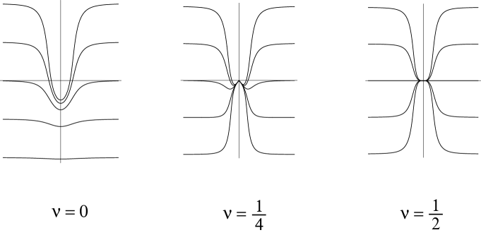
Figure 5.3: Solutions to the BPS equation Eq. (5.3.27) for $a=1$. The vertical axis displays $z\equiv-r\cos\theta$. A D5-brane with asymptotic value $z_{\infty}>0$ is connected to the $N$ D3-branes at the origin of the plot by $(1-\nu)N$ strings. A D5-brane with asymptotic value $z_{\infty}<0$ is connected to the D3-branes by $-\nu N$ strings (the sign denotes the orientation of the strings). The fact that the number of strings jumps by $N$ as a D5-brane is dragged upwards from negative to positive $z_{\infty}$ is related to the Hanany-Witten effect [76].

These solutions are labelled by $\nu$ (introduced in Eq. (5.3.17)) and by the asymptotic value $z_{\infty}$ of $z\equiv-r\cos\theta$ (see Fig. 5.3).

Since the $a=0$ background can be considered as the $r\rightarrow 0$ limit of the $a=1$ background, one expects the solutions for $a=0$ and $a=1$ to approximately coincide for small $r$. Indeed, it was observed in [78] that this is indeed the case if the parameters $c$ and $z_{\infty}$ are related by

$$c=\left(\frac{R^{4}}{2|z_{\infty}|}\right)^{1/3}\leavevmode\nobreak\ .$$ (5.3.32)

The condition that the second inequality in Eq. (5.3.26) be saturated states that ${\cal{Z}}_{\rm el}$ should not change sign in the integration region in Eq. (5.3.24). When Eq. (5.3.27) holds, the sign of ${\cal{Z}}_{\rm el}$ is determined by the sign of

$$\Delta\cos\theta-\Pi\sin\theta=a\,r^{4}\,\sin^{4}\theta\,\cos\theta+\frac{3}{2}\,R^{4}\,\sin\theta\,\eta(\theta)\,,$$ (5.3.33)

where the function $\eta$ is defined in Eq. (5.3.28). For $a=0$, we precisely recover the condition that $\eta$ should have definite sign. (We have not done the analysis for $a=1$.)

The remainder of this chapter is devoted to the physical interpretation of $Z_{\rm el}$. It follows from Eq. (5.3.22) that

$$Z_{\rm el}=\left[\Pi\,r\cos\theta\right]_{\theta_{i}}^{\theta_{f}}+\left[\left(\frac{a}{5}+\frac{R^{4}}{r^{4}}\right)(r\sin\theta)^{5}\right]_{\theta_{i}}^{\theta_{f}}\leavevmode\nobreak\ .$$ (5.3.34)

We shall evaluate this expression for the solutions of Eq. (5.3.27), displayed in Fig. 5.2 and Fig. 5.3.

In the case $a=0$, the second term in Eq. (5.3.34) vanishes for all the solutions of Eq. (5.3.27), as is suggested by Fig. 5.2. Using Eq. (5.3.17) and restoring the factor $T_{5}\,V_{(4)}/\kappa$, the first term gives the divergent result

$$Z_{\rm el}=(1-\nu)NTL\leavevmode\nobreak\ ,$$ (5.3.35)

where $T$ is the tension of a fundamental string and $L$ is the (infinite) coordinate distance between the D3-branes at the origin of Fig. 5.2 and the “upper end” of the D5-brane. However, the interpretation of this divergence is clear: it is the tension of $(1-\nu)N$ infinitely extended fundamental strings.

For $a=1$, the second term in Eq. (5.3.34) is infinite. However, this infinity is to be expected for an infinitely extended D-brane. In fact, it precisely equals the energy of an unexcited D5-brane whose world-space is the $\theta=\pi/2$ hyperplane in the transverse space to the D3-branes. Indeed, for such a D5-brane one computes

$$E\equiv E_{0}=\int_{\Sigma}d^{5}\sigma\,\sqrt{-\det\hat{G}}=\int_{0}^{r_{f}}dr\,r^{4}\,H(r)=\left[\left(\frac{a}{5}+\frac{R^{4}}{r^{4}}\right)\,r^{5}\right]_{0}^{r_{f}},$$ (5.3.36)

which agrees with the second term in Eq. (5.3.34) evaluated for the solutions in Fig. 5.3. We shall just subtract the infinite second term in Eq. (5.3.34) from the energy and study the deformation energy $E_{\rm def}$:

$$E=E_{0}+E_{\rm def}\leavevmode\nobreak\ .$$ (5.3.37)

Thus, for $a=1$ we rewrite the bound Eq. (5.3.25) as

$$E_{\rm def}\geq Z_{9}\leavevmode\nobreak\ ,$$ (5.3.38)

where

$$Z_{9}\equiv\left[\Pi\,r\cos\theta\right]_{\theta_{i}}^{\theta_{f}}=(\frac{1}{2}-\nu)NTz_{\infty}.$$ (5.3.39)

Here, we have used Eq. (5.3.17) and the solutions in Fig. 5.3. To interpret $Z_{9}$, note that for $z_{\infty}>0$, $Z_{9}$ corresponds to the tension of $(1/2-\nu)N$ strings stretched between the D5-brane and the D3-branes. At first sight, this might seem to be in contradiction with the fact that there are really $(1-\nu)N$ strings between the D5-brane and the D3-branes. However, remember that an unexcited D5-brane is connected to the D3-branes via $N/2$ strings. Thus, one can imagine that $N/2$ of the $(1-\nu)N$ strings are needed to bring the D5-brane in its unexcited state and that only the remaining $(1/2-\nu)N$ strings exert a force on the D5-brane. By the way, note that this force is not sufficient to make the infinitely heavy D5-brane move: we are really studying static configurations.

To motivate the name $Z_{9}$, note that, from the ten-dimensional spacetime point of view, we have been studying the triple intersection

$$\begin{array}[]{ccccccccccl}{\rm D3}:&1&2&3&\_&\_&\_&\_&\_&\_&\quad\mbox{background}\\ {\rm D5}:&\_&\_&\_&4&5&6&7&8&\_&\quad\mbox{world-volume}\\ {\rm F1}:&\_&\_&\_&\_&\_&\_&\_&\_&9&\quad\mbox{BPS solution.}\end{array}$$

In our analysis, the D3-branes are the background and the F1 plays the role of a soliton of the D5-brane world-volume theory. We have chosen the name $Z_{9}\!$ because of the direction in which the string stretches.

In our paper [9], further evidence is provided in favour of the interpretation of $Z_{9}$ (or $Z_{\rm el}$ in the case $a=0$) as a charge associated to fundamental strings ending on the D5-brane world-volume. The additional evidence consists in the fact that $Z_{9}$ (or $Z_{\rm el}$) has the right quantum numbers to appear as a central charge in the D5-brane world-volume supersymmetry algebra. We refer the reader to [9] for details. The analysis presented in this section has been generalized to other configurations of intersecting branes in [78, 81].

Chapter 6 Type 0 string theory

In this chapter, we study some aspects of type 0 string theory [82]. Compared to type II strings, type 0 strings have a tachyon, twice as many R-R fields and no spacetime fermions in their perturbative spectra. Because of the problems related to the presence of a tachyon, type 0 string theory became popular only one year and a half ago. Then, it was noticed [83, 84] that the tachyon may not be a big problem when one is interested in D-brane world-volume field theories, as in the AdS/CFT correspondence. In Section 6.1, we give a brief review of this motivation to study type 0 string theory. Type 0 string theory has also been studied by itself, which has led to some interesting speculations about type 0 dualities [85].

In this chapter, we study the main building blocks in these developments: type 0 strings, D-branes and NS-fivebranes. In particular, we derive the D-brane Wess-Zumino action [10], determine the massless spectrum of NS-fivebranes [15] and combine these ingredients to comment [15] on a type 0 duality [85].

In Section 6.2, we introduce type 0 strings and compare them to type II strings [82]. In Section 6.3, we introduce type 0 D-branes [86, 84]. As could be anticipated from the doubling of the R-R spectrum compared to type II string theory, the number of different D-branes is also doubled. Following our paper [10], we derive a Wess-Zumino action for type 0 D-branes. We use an anomaly inflow argument very similar to the one used for type II D-branes. Again, the different terms in the Wess-Zumino action can be checked via boundary state computations.

In Section 6.4, which is based on our paper [15], we study NS fivebranes in type 0 string theory. We derive their massless spectra and find that they are non-chiral and purely bosonic for both type 0A and type 0B. Type IIA NS fivebranes have a chiral, anomalous spectrum. The anomaly is cancelled by anomaly inflow from the bulk of spacetime. We compute that for both type 0A and type 0B there is no such inflow from the bulk. This is consistent with the non-chiral and thus non-anomalous spectra of type 0 NS fivebranes. We propose a speculative interpretation of the type 0 NS fivebrane spectra in terms of “type 0 little strings”.

In Section 6.5, we combine our studies of type 0 D-branes and NS fivebranes to comment [15] on the recently proposed type 0B S-duality [85].

One of the themes in our studies of type 0 string theories is that, although they are not supersymmetric, they resemble the supersymmetric type II theories in many respects. A striking example is the analysis of Section 6.3.1 [10]. However, we have to stress that, due to the presence of a tachyonic mode in the bulk of spacetime, the results presented in this chapter are on a less firm footing than the analogous ones in type II.

6.1 Introduction

In Section 5.1.1, we indicated how string theory can be used to study the strong coupling limit of ${\cal N}=4$ SU($N$) super-Yang-Mills theory in 3+1 dimensions. Interesting as it is, studying the strong coupling limit of a supersymmetric gauge theory is not the final aim of high energy physics. One of the real interests is non-supersymmetric gauge theory. There have been several approaches towards this aim. In this section, we briefly introduce one that is based on type 0 string theories.

At the end of Section 3.1.1, we restricted ourselves to supersymmetric string theories. These theories satisfy consistency conditions like modular invariance, and are free of tachyons, excitations with negative mass squared. However, there also exist modular invariant non-supersymmetric string theories. Two of them are the type 0A and type 0B closed string theories, to be introduced in Chapter 6. They differ from the type IIA and type IIB string theories in that they have different GSO projections. The main differences with the type II theories are that the type 0 theories have a doubled R-R spectrum, a tachyon and no spacetime fermions.

The presence of a tachyon means that one is doing perturbation theory around an unstable “vacuum”. This obviously makes it hard to do computations in these theories. Nevertheless, the presence of a tachyon does not imply that the theories are irrelevant to physics: it may well be that the tachyon potential has a stable minimum in which the tachyon can condense. This, in turn, raises another problem: determining the tachyon potential requires off-shell information, which is not available in perturbative string theory.

Despite these problems, one can guess an off-shell extrapolation of on-shell results and check the internal consistency of the resulting proposal. This is what Klebanov and Tseytlin did in [84]. They argued that in certain backgrounds with a large five-form R-R flux the tachyonic instability may be cured.

Like the R-R spectrum, the number of different D-branes is doubled in type 0 with respect to type II. For instance, D3-branes can be electrically or magnetically charged under the unconstrained five-form R-R field strength. The configuration studied in [84] involves a configuration of coincident electric D3-branes. In the spirit of Maldacena’s conjecture, it is proposed that the field theory living on the D-branes has a string theory dual. A crucial observation is that, although there is a closed string tachyon in the bulk of the ten-dimensional spacetime, the field theory on the branes (describing the low-energy excitations of the open strings ending on them) is tachyon-free. Thus, one may hope that D-branes will be stable objects once the closed string tachyon has condensed.

The field theory one finds in this way is non-supersymmetric, non-conformal (in fact, asymptotically free) and tachyon-free [84, 87, 88].

One can also study stacks of an equal number of electric and magnetic D3-branes [89], giving rise to field theories that are conformally invariant in the limit of a large number of branes. We shall not go into these theories here, though we refer the reader to our paper [10], where we study an orbifold of these models.

Type 0 string theories have also been studied independently of the AdS/CFT correspondence. In particular, there have been some interesting type 0 duality conjectures, one of which will be examined in Section 6.5. It is unclear how to deal with the tachyonic instability of type 0 string theory in a flat background. Our point of view is that arguments based on anomaly cancellation may be robust under continuous deformations of the theory. Therefore, one may hope that, even though the background one is expanding around is unstable, one could be able to extract useful information from such anomaly arguments. However, we repeat that the whole chapter is highly conjectural.

6.2 Strings: from type II to type 0

In the Neveu-Schwarz-Ramond formulation, type II string theories are obtained by imposing independent GSO projections on the left and right moving part. This amounts to keeping the following (left,right) sectors:

$${\rm IIB:} (NS+,NS+)\ ,\leavevmode\nobreak\ \leavevmode\nobreak\ (R+,R+)\ ,\leavevmode\nobreak\ \leavevmode\nobreak\ (R+,NS+)\ ,\leavevmode\nobreak\ \leavevmode\nobreak\ (NS+,R+)\leavevmode\nobreak\ ;$$

$${\rm IIA:} (NS+,NS+)\ ,\leavevmode\nobreak\ \leavevmode\nobreak\ (R+,R-)\ ,\leavevmode\nobreak\ \leavevmode\nobreak\ (R+,NS+)\ ,\leavevmode\nobreak\ \leavevmode\nobreak\ (NS+,R-)\leavevmode\nobreak\ ,$$

where for instance R+ and R- are the Ramond sectors projected with $P_{\rm GSO}=(1+(-)^{F})/2$ and $P_{\rm GSO}=(1-(-)^{F})/2$, respectively, $F$ being the world-sheet fermion number (see Section 3.1.1).

There is another, equivalent choice for both theories (related to the first choice by a spacetime reflection):

$${\rm IIB^{\prime}:} (NS+,NS+)\ ,\leavevmode\nobreak\ \leavevmode\nobreak\ (R-,R-)\ ,\leavevmode\nobreak\ \leavevmode\nobreak\ (R-,NS+)\ ,\leavevmode\nobreak\ \leavevmode\nobreak\ (NS+,R-)\leavevmode\nobreak\ ;$$

$${\rm IIA^{\prime}:} (NS+,NS+)\ ,\leavevmode\nobreak\ \leavevmode\nobreak\ (R-,R+)\ ,\leavevmode\nobreak\ \leavevmode\nobreak\ (R-,NS+)\ ,\leavevmode\nobreak\ \leavevmode\nobreak\ (NS+,R+)\leavevmode\nobreak\ .$$

For the massless R-R sector, the difference between the primed and unprimed theories shows up in opposite chiralities of the bi-spinor containing the R-R field strengths. This implies a sign difference in the Hodge duality relations among these field strengths, resulting in a selfdual five-form field strength in IIB and an antiselfdual one in IIB’, for instance.

The type 0 string theories contain instead the following sectors:

$${\rm 0B:} (NS+,NS+)\ ,\leavevmode\nobreak\ \leavevmode\nobreak\ (NS-,NS-)\ ,\leavevmode\nobreak\ \leavevmode\nobreak\ (R+,R+)\ ,\leavevmode\nobreak\ \leavevmode\nobreak\ (R-,R-)\leavevmode\nobreak\ ;$$

$${\rm 0A:} (NS+,NS+)\ ,\leavevmode\nobreak\ \leavevmode\nobreak\ (NS-,NS-)\ ,\leavevmode\nobreak\ \leavevmode\nobreak\ (R+,R-)\ ,\leavevmode\nobreak\ \leavevmode\nobreak\ (R-,R+)\leavevmode\nobreak\ .$$

Here are some differences between type 0 and type II string theory. First, type 0 theories do not contain bulk spacetime fermions, which would have to come from “mixed” (R,NS) sectors. Second, the inclusion of the NS-NS sectors with odd fermion numbers means that the closed string tachyon is not projected out. Third, the type 0 R-R spectrum is doubled compared to type II: the R-R potentials of the primed and unprimed type II theories are combined, resulting for instance in an unconstrained five-form field strength in type 0B.

We shall summarize the spectra of type 0 versus type II string theories in a table at the end of Section 6.4.3.

6.3 D-branes

D-branes in type 0 theories have been discussed in [86] and [84]. First, we mainly review some of their results. Then, in Section 6.3.1, we present a result from our paper [10].

Because of the doubling of the R-R spectrum, in type 0B there are two kinds of D3-branes, named electric and magnetic in contrast to the selfdual D3-brane of type IIB.

A configuration with equal numbers of coincident electric and magnetic branes is reminiscent of type II branes, which have been well studied. It will turn out that many results can be transferred to type 0 almost without effort. For instance, we shall see in Section 6.3.1 that chiral fermions are present on certain intersections of electric and magnetic branes, leading to anomaly inflow on the intersection via anomalous D-brane couplings. These, in turn, lead to the creation of a string when certain D-branes cross each other.

As discussed in Section 6.2, the spectrum of type 0 theories contains two ($p+1$)-form R-R potentials for each even (0A) or odd (0B) $p$. We will denote these by $C_{p+1}$ and $C^{\prime}_{p+1}$, referring to the unprimed and primed type II theories mentioned above. For our purposes, more convenient combinations are

$$(C_{p+1})_{\pm}=\frac{1}{\sqrt{2}}(C_{p+1}\pm C^{\prime}_{p+1})\leavevmode\nobreak\ .$$ (6.3.1)

For $p=3$, these are the electric ($+$) and magnetic ($-$) potentials [84]. We will adopt this terminology also for other values of $p$.

There are four types of “elementary” D-branes for each $p$: an electric and a magnetic one, i.e. charged under $(C_{p+1})_{\pm}$, and the corresponding antibranes. In [84], the interaction energy of two identical parallel ($p+1$)-branes was derived by computing the relevant cylinder diagram (see Fig. 6.1) in the open string channel, analogously to the Polchinski computation [47] in type II.

Figure 6.1: The cylinder diagram between two D-branes can be interpreted in two different ways. In the open string channel, i.e., if $\sigma$ is treated as the world-sheet time coordinate, it represents a one-loop vacuum diagram. In the closed string channel, i.e., if $\tau$ is treated as the world-sheet time coordinate, it is a tree-level diagram: the two D-branes exchange a closed string. One can derive the charges of D-branes by computing cylinder diagrams in the open string channel and imposing that the result should be reproduced in the closed string channel.

Isolating, via modular transformation, the contributions due to the exchange of long-range fields in the closed string channel, it is found on the one hand that the tension of these branes is a factor $\sqrt{2}$ smaller than for type II branes. On the other hand, the R-R repulsive force between two like branes has twice the strength of the graviton-dilaton attraction [84]; thus, the type 0 branes couple to the corresponding R-R potentials $(C_{p+1})_{\pm}$ with the same charge as the branes in type II couple to the potential $C_{p+1}$.

The cylinder diagram between two D-branes in type II can also be considered as a tree-level diagram in which a closed string propagates between two “boundary states”. Recall from Section 4.1 that a boundary state is a particular BRST invariant closed string state that describes the emission of a closed string from a D-brane. It satisfies conditions that correspond to the boundary conditions for open strings ending on the D-brane. In particular, for the fermionic fields $\psi^{\mu}$ the boundary state $|{B,\eta}\rangle_{\rm NS,R}$, which depends on the sector, R or NS, and on an additional sign $\eta=\pm$, satisfies

$$(\psi^{\mu}-\eta S^{\mu}_{\leavevmode\nobreak\ \nu}\tilde{\psi}^{\nu})|{B,\eta}\rangle_{\rm NS,R}=0\leavevmode\nobreak\ ,$$ (6.3.2)

where $S^{\mu}_{\leavevmode\nobreak\ \nu}$ is diagonal, with entries $1$ in the worldvolume and $-1$ in the transverse directions. In type II theories, the GSO projection requires a mixture of the two choices $\eta=\pm 1$. Indeed, starting, for instance, with $\eta=+1$, one finds that the type II boundary state $|{B}\rangle$ $=P_{\rm GSO}|{B,+}\rangle_{\rm NS}$ $\oplus P_{\rm GSO}|{B,+}\rangle_{\rm R}$ is

$$|{B}\rangle={1\over 2}\left((|{B,+}\rangle_{\rm NS}-|{B,-}\rangle_{\rm NS})\oplus(|{B,+}\rangle_{\rm R}+|{B,-}\rangle_{\rm R})\right)\leavevmode\nobreak\ .$$ (6.3.3)

We remark that in the case of type 0 D-branes, the various cylinder amplitudes between an electric (or magnetic) D-brane and an electric (or magnetic) D-brane can simply be reproduced using the following unprojected (and differently normalized) boundary states, whose sum is $\sqrt{2}$ times the type II boundary state:

$$|{B,\pm}\rangle=\frac{1}{\sqrt{2}}\left(\pm|{B,\pm}\rangle_{\rm NS}\oplus|{B,\pm}\rangle_{\rm R}\right)\leavevmode\nobreak\ .$$ (6.3.4)

Here, $|{B,+}\rangle$ represents an electric brane and $|{B,-}\rangle$ a magnetic one.

As a cross-check, with these boundary states one can compute the one-point function on the disc of a R-R potential (as in [45]). Denoting by ${}_{\pm}\langle{C_{p+1}}|$ the out-state corresponding to the $(C_{p+1})_{\pm}$ potentials, the one-point function describing its coupling to a type 0 D$p$-brane will be ${}_{\pm}\langle{C_{p+1}}|{B,\pm}\rangle$. As one can see from Eq. (6.3.1), Eq. (6.3.3) and Eq. (6.3.4), this gives indeed the same charge as in type II, where one would compute $\langle{C_{p+1}}|{B}\rangle$.

6.3.1 Anomaly inflow and Wess-Zumino action

The D-branes we have just described show many similarities to their type II cousins. In this section, we will push the analogy further to include the whole Wess-Zumino action, i.e., all the anomalous D-brane couplings.

The open strings stretching between two like branes are bosons, just like the bulk fields of type 0. However, fermions appear from strings between an electric and a magnetic brane [86]. Thus, one could wonder whether there are chiral fermions on the intersection of an electric and a magnetic brane. Consider such an orthogonal intersection with no overall transverse directions. If the dimension of the intersection is two or six, a cylinder computation reveals that there are precisely enough fermionic degrees of freedom on the intersection to form one chiral fermion.

In type II string theory, the analogous computation shows that chiral fermions are present on two- or six-dimensional intersections of two orthogonal branes with no overall transverse directions. That observation has far-reaching consequences. As we discussed in Section 3.5.1, the presence of chiral fermions leads to gauge and gravitational anomalies on those intersections of D-branes [50]. In a consistent theory, such anomalies should be cancelled by anomaly inflow [21]. In the present case, the anomaly inflow is provided by the anomalous D-brane couplings in the Wess-Zumino part of the D-brane action [50, 51]. These anomalous couplings have an anomalous variation localized on the intersections with other branes.

A careful analysis of all the anomalies [51] shows that the anomalous part of the D$p$-brane action is given, in terms of the formal sum $C$ of the various R-R forms, by

$$S_{\rm WZ}=\frac{T_{p}}{\kappa}\int_{p+1}C\wedge e^{2\pi\alpha^{\prime}\,F+B}\wedge\sqrt{\hat{A}(R_{T})/\hat{A}(R_{N})}\leavevmode\nobreak\ \leavevmode\nobreak\ .$$ (6.3.5)

Here, $T_{p}/\kappa$ denotes the D$p$-brane tension, $F$ the gauge field on the brane and $B$ the NS-NS two-form. Further, $R_{T}$ and $R_{N}$ are the curvatures of the tangent and normal bundles of the D-brane world-volume, and $\hat{A}$ denotes the A-roof genus. We refer to Section 3.4 for details on the action Eq. (6.3.5).

These anomalous D-brane couplings have various applications. To mention just one, using T-duality it has been argued [90] that they imply the creation of a fundamental string whenever certain type II D-branes cross each other. This string creation process is dual to the Hanany-Witten effect [76].

Let us now return to type 0 string theory. As stated above, here chiral fermions live on intersections of electric and magnetic type 0 D-branes. The associated gauge and gravitational anomalies on such intersections match the ones for type II D-branes. To cancel them, the minimal coupling of a D$p$-brane to a ($p+1$)-form R-R potential should be extended to the following Wess-Zumino action [10]:

$$S_{\rm WZ}=\frac{T_{p}}{\kappa}\int_{p+1}(C)_{\pm}\wedge{\rm e}^{2\pi\alpha^{\prime}\,F+B}\wedge\sqrt{\hat{A}(R_{T})/\hat{A}(R_{N})}\leavevmode\nobreak\ .$$ (6.3.6)

The $\pm$ in Eq. (6.3.6) distinguishes between electric and magnetic branes. Note that $T_{p}/\kappa$ denotes the tension of a type II D$p$-brane, which is $\sqrt{2}$ times the type 0 D$p$-brane tension.

The argument that the variation of this action cancels the anomaly on the intersection is a copy of the one described above in the type II case, apart from one slight subtlety. For definiteness, consider the intersection of an electric D5-brane (denoted D5₊) and a magnetic D$5$-brane (D5_-) on a string (see Fig. 6.2).

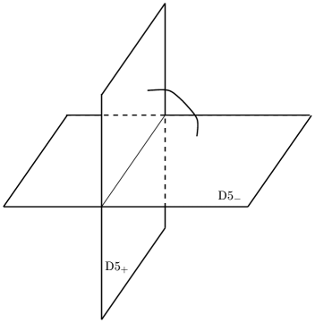
Figure 6.2: Electric and magnetic D5-branes intersecting on a string. The open strings stretching from one brane to the other give rise to chiral fermions living on the intersection.

Varying the electric D$5$-brane action (exhibiting the $(C_{2})_{+}$ potential, or rather, its field strength $(\tilde{F}_{3})_{+}$), one finds that the variation is localized on the intersection of the electric D$5$-brane with branes charged magnetically under the $(\tilde{F}_{3})_{+}$ field strength. Using Eq. (6.3.1), the different behaviour under Hodge duality of the R-R field strengths of type II and II’ shows that these are precisely the branes carrying (electric) $(\tilde{F}_{7})_{-}$ charge, i.e., what we called the magnetic D$5$-branes. Schematically,

$$\delta\int_{{\rm D}5_{+}}\,I_{3}^{(0)}\wedge(\tilde{F}_{3})_{+} = -\int_{{\rm D}5_{+}}\,I_{2}^{(1)}\wedge d(\tilde{F}_{3})_{+}$$ (6.3.7)

$$= -\int_{{\rm D}5_{+}}\,I_{2}^{(1)}\wedge d*(\tilde{F}_{7})_{-}$$

$$= -\int_{{\rm D}5_{+}}\,I_{2}^{(1)}\wedge\delta_{{\rm D}5_{-}}\leavevmode\nobreak\ .$$

A completely analogous discussion goes through for the variation of the magnetic D$5$-brane action.

This anomaly inflow argument fixes (the anomalous part of) the Wess-Zumino action, displayed in Eq. (6.3.6). The presence of these terms (and of a similar non-anomalous one [8]) can be checked by a disc computation, as in type II [7, 12, 8], see Chapter 4. In fact, the computation is practically the same, confirming the form of the action Eq. (6.3.6).

Assuming T-duality to hold between type 0A/B, the arguments of [90] indicate the creation of a fundamental string when certain electric and magnetic branes cross each other. In type II, this is linked to the Hanany-Witten effect [76] by a chain of dualities. However, this chain involves type IIB S-duality. It is not clear whether S-duality exists in type 0B string theory (see Section 6.5).

The conclusion of Section 6.3 is that type 0 D-branes are similar to type II D-branes. In particular, their interaction with R-R potentials is described by the Wess-Zumino action Eq. (6.3.6).

6.4 NS-fivebranes

This section is based on our paper [15]. First, we derive the spectra of type 0 NS5-branes using T-duality. These spectra are non-chiral for both type 0A and type 0B. Then, we check that this non-chirality is consistent with anomaly considerations. Finally, we propose a speculative interpretation of these spectra in terms of “type 0 little strings”.

6.4.1 NS fivebrane spectra

In type II string theories, the massless spectrum on NS5-branes can be derived via an analysis of the zero-modes of the classical supergravity NS5-brane solutions [52]. We will find it convenient to do the analysis for the T-dual objects, since there the geometrical interpretation is manifest.

Under T-duality, the type IIA/B NS5-branes are mapped to type IIB/A Kaluza-Klein (KK) monopoles (see, for instance, [91]). A KK monopole is described by a supergravity solution with six worldvolume directions and a Euclidean Taub-NUT (ETN) metric in the transverse space [92]. The massless fields on the KK monopole correspond to the zero-modes of the bulk supergravity fields on ETN. The normalizable harmonic forms on ETN consist of one selfdual two-form [93]. In the NS-NS sector, there are three zero-modes from broken translation invariance and one scalar from the NS two-form. These four scalars correspond to the translation zero-modes on the corresponding NS5-branes. The R-R fields give additional bosonic zero-modes: on the IIB KK monopole, the R-R two-form gives rise to a scalar and the selfdual R-R four-form potential leads to a selfdual two-form; the IIA KK monopole has a vector coming from the R-R three-form. In addition, there are fermionic zero-modes from broken supersymmetry: two fermions with opposite chirality for the IIA KK monopole and of the same chirality for IIB.

All in all, this leads to an ${\cal N}=(2,0)$ tensor multiplet on the IIA NS5 and an ${\cal N}=(1,1)$ vector multiplet on the IIB NS5.

Repeating this analysis for type 0 NS5-branes, it is clear that the fermionic zero-modes disappear (because there are no fermions in the bulk). Nothing changes as far as the NS-NS zero-modes are concerned, but from the R-R fields we find extra zero modes from the doubled R-R spectrum in the bulk. On the 0B NS5, there is an extra vector (compared to the IIB NS5), whereas the 0A NS5 gets an extra scalar and an anti-selfdual tensor. In particular, the spectrum is non-chiral on both branes.

Note that, although type 0 NS5-branes are not supersymmetric, their massless spectra consist of the bosonic part of ${\cal N}=2$ supermultiplets. At the end of Section 6.4.3, we shall summarize the massless spectra of type II and type 0 NS5-branes in a table.

6.4.2 Absence of anomalies

We discussed in Section 3.5.2 that at one string loop the type IIA tree level supergravity action is supplemented with the Wess-Zumino type term $\int B\wedge X_{8}(R)$ coupling the NS-NS two-form $B$ to four gravitons. $X_{8}$ is a quartic polynomial in the spacetime curvature two-form. The original derivation of this one-loop term [54] provided a non-trivial consistency check for six-dimensional heterotic-type II duality. Apart from that, this specific piece of the action is also responsible for gravitational anomaly cancellation on IIA NS fivebranes [53].

Let us first highlight some aspects of the direct calculation in type II, which will enable us to draw conclusions about the analogous type 0 amplitude almost without effort. First, as the interaction contains the ten-dimensional $\epsilon$ symbol, only odd spin structures on the torus can contribute, i.e., either the left-moving or the right-moving fermions but not both, have to be in the odd spin structure. Furthermore, the even spin structures are summed over to achieve modular invariance. From a different perspective, this may also be seen as performing the GSO projection on the closed string states in the loop [94]. In a Hamiltonian framework, the torus vacuum diagram is written as a trace over the closed string Hilbert space, which decomposes in four different sectors as in Eq. (6.2). Chiral traces over these sectors can be expressed in terms of traces over fermion sectors with periodic (P) or antiperiodic (A) boundary conditions in the ($\sigma$,$\tau$) world-sheet directions:

$${\rm Tr}_{(NS,-)} = \frac{1}{2}\left((A,A)-(A,P)\right)\ ;$$

$${\rm Tr}_{(NS,+)} = \frac{1}{2}\left((A,A)+(A,P)\right)\ ;$$

$${\rm Tr}_{(R,-)} = \frac{1}{2}\left((P,A)-(P,P)\right)\ ;$$

$${\rm Tr}_{(R,+)} = \frac{1}{2}\left((P,A)+(P,P)\right)\ .$$

Notice that the odd $(P,P)$ spin structure only occurs in the Ramond sector. From the GSO-projected spectrum in Eq. (6.2), only (R,NS) and (R,R) sectors contain (odd,even) pieces, yielding

$$\frac{1}{4}\left((P,P),(A,A)+(A,P)+(P,A)\right)\ .$$ (6.4.1)

The right-moving combination is modular invariant, and in fact vanishes as a consequence of Jacobi’s “abstruse identity”. If one calculates the amplitude for one B-field and four gravitons, one inserts vertex operators in the appropriate pictures. Still, the right-moving even structures are summed over as in Eq. (6.4.1). In contrast with the partition function, however, in this case a non-vanishing result is found [54]. It is also argued there that in type IIB the (odd,even) and (even,odd) contributions cancel out whereas they add in type IIA. So only in the latter case is the probed interaction present.

This difference between type IIA and IIB could have been inferred from their respective NS fivebrane worldvolume spectra, a chiral one in type IIA and a non-chiral one in type IIB. The chiral spectrum suffers from a gravitational anomaly in six dimensions, which is neatly cancelled by the standard anomaly inflow [21] from the bulk through the above derived coupling [53].

Let us repeat the argument for the one-loop correlator in type 0 string theories. Now, it is only (R,R) sectors that contribute to the (odd,even) piece in the one-loop partition function, yielding

$$\frac{1}{4}\left((P,P)-(P,P),(P,A)\right)$$ (6.4.2)

both for 0A and 0B. As in type II, one may now wish to insert vertex operators. However, it is obvious that the obligatory sum over spin structures as in Eq. (6.4.2) now yields a vanishing result for the (odd,even) part by itself. Analogously, the (even,odd) part will vanish by itself. Whence the absence of the anomaly-cancelling term in both type 0A and 0B.

Reversing the anomaly inflow argument, in type 0A the selfdual two-form must be supplemented with an anti-selfdual two-form, in order not to give rise to gravitational anomalies. This nicely agrees with the unconstrained two-form on the NS fivebrane, derived in Section 6.4.1. From T-duality, an additional vector (compared to the IIB NS5-brane) is then to be expected on the type 0B NS5-brane, which is also consistent with Section 6.4.1.

6.4.3 A little string interpretation

In type II string theories, the fivebrane worldvolume theories have been conjectured to be properly described by “little strings”[95]. These non-critical closed string theories have hitherto remained mysterious, although some qualitative features may be understood. We briefly recall some of these, focusing on the type IIB case. However, we prefer first to treat the more familiar example of a fundamental string, providing a guiding reference when dealing with the little strings.

A fundamental string solution in supergravity breaks half of the 32 bulk supersymmetries. These broken symmetries give rise to fermion zero-modes on the string, of which 8 are left-moving and 8 right-moving. They are identified with the Green-Schwarz space-time fermion fields on the world-volume. Upon quantization of these fermions, 128 bosons and 128 fermions are found, together building the on-shell ${\cal N}$ = 2 supergravity multiplet. This multiplet is also found in the RNS formalism used in this thesis, so the picture is consistent. In the latter formulation, it is not hard to see that the NS-NS sector fields together with, say, the R-NS sector build an ${\cal N}$ = 1 supergravity multiplet. Likewise, the NS-R and R-R sector are combined into one multiplet of ${\cal N}$ = 1.

Let us move on now to little strings. One way to derive properties of little strings in type IIB is to consider a gauge instanton on a D5 brane. Half of the bulk supersymmetries are unbroken by the D5-brane. Sixteen real supercharges are thus found, obeying an ${\cal N}$=(1,1) superalgebra. Of the sixteen supersymmetries, half are broken by the instanton. On the macroscopic string, there are thus eight fermionic modes, four left-moving and four right-moving ones. Upon quantization of these zero-modes, one finds 8 bosonic and 8 fermionic states. They correspond to the on-shell degrees of freedom of one ${\cal N}$=(1,1) vectormultiplet. Upon decomposition with respect to ${\cal N}$ = 1 six-dimensional supersymmetry, one hypermultiplet and one vectormultiplet result. It is conceivable that a similar analysis in type IIA, if possible at all, would give a ${\cal N}$=(2,0) tensormultiplet, decomposing into one hypermultiplet and one tensormultiplet of ${\cal N}$=1 supersymmetry. We remark that the tensormultiplet has a bosonic content that consists of one scalar and one two-form potential with self-dual field strength.

All in all, one may wish to draw the following analogies between type ii little strings and type II strings. In both cases, there is one universal sector, the hypermultiplet resp. the (NS-NS + R-NS) sector. The other sector depends on whether or not the supersymmetry in the “bulk” is chiral, where “bulk” means the fivebrane worldvolume for the little string and ten-dimensional spacetime for the type II string. For the non-chiral type IIA and little type iia, the remaining bosonic fields are odd $q$-form potentials, coupling to even $p$ D$p$- resp. d$p$-branes. As to chiral type IIB/iib, the R-R sector has only even $q$-form potentials, of which one has a self-dual field strength. In these theories, only odd $p$ D$p$ or d$p$-branes occur. So this analogy, however formal, is at least remarkable. We shall visualize it in the tables at the end of this section.

As to the various fivebranes, the type IIA NS fivebrane theory is conjectured to be described by chiral iib little strings, whereas iia little strings would do the job for type IIB fivebranes.

One may then proceed and construct “little type 0a/b strings” by mimicking the procedure for the bulk strings: spacetime fermions are removed and there is a doubled R-R spectrum compared to the superstring. Concretely, this would imply that the massless spectrum of little type 0a strings consists of the bosonic contents of one hypermultiplet and two vectormultiplets, in ${\cal N}$=1 language. This precisely matches with the spectrum on the type 0B NS fivebrane. Little type 0b strings would then generate the bosonic content of one hypermultiplet, one selfdual tensormultiplet and one anti-selfdual tensormultiplet. Also here, this seems to be consistent with the spectrum of the type 0A NS fivebrane.

In the following tables, we summarize the spectra of type II versus type 0 string theories

	II		0
	A	B	A	B
Universal	$g_{\mu\nu},B_{\mu\nu},\Phi$		$g_{\mu\nu},\,B_{\mu\nu},\,\Phi$
sector	+ fermions
Other	$C_{1},\,C_{3}$	$C_{0},\,C_{2},\,C_{4}^{+}$	$C_{1},\,C_{1}^{\prime},\,C_{3},\,C_{3}^{\prime}$	$C_{0},\,C_{0}^{\prime},\,C_{2},$
sector	+ fermions	+ fermions		$C_{2}^{\prime},\,C_{4}^{+},\,C_{4}^{-}$
	(non-chiral)	(chiral)	(non-chiral)	(non-chiral)

and of type ii versus type o little string theories:

	ii		o
	a	b	a	b
Universal	4 scalars		4 scalars
sector	+ fermions
Other	vector	$T_{2}^{+}$, scalar	2 vectors	$T_{2}^{+},\,T_{2}^{-}$,
sector	+ fermions	+ fermions		2 scalars
	(non-chiral)	(chiral)	(non-chiral)	(non-chiral)

To summarize Section 6.4, we have derived the massless spectra of type 0 NS5-branes. We have shown that they are consistent with anomaly considerations. We have proposed a speculative interpretation of the spectra in terms of “type 0 little strings”.

6.5 Type 0B S-duality

In this section, we combine results from Section 6.3.1 and Section 6.4 to comment [15] on the type 0B S-duality conjectured in [85].

Strings

In type IIB string theory, the fundamental string is mapped to the D-string under S-duality. The Green-Schwarz light-cone formulation of the fundamental type IIB string involves eight spacetime bosonic fields and sixteen spacetime fermionic ones. All fermions transform in the ${\bf 8}_{s}$ representation of the transverse SO(8) rotation group. Upon quantization, their zero-modes generate the 256-fold degenerate groundstate, transforming in the $({\bf 8}_{v}+{\bf 8}_{c})\otimes({\bf 8}_{v}+{\bf 8}_{c})$ of SO(8).

The excitations of a D1-brane can be described in string perturbation theory by quantizing the open strings beginning and ending on it. Doing so, the NS sector gives eight massless bosons and the R sector sixteen massless fermions.

Note that these massless excitations of both the fundamental string and the D-string can be interpreted as Goldstone modes for broken translation invariance and broken supersymmetry.

It is believed that the IIB D-string at strong (fundamental) string coupling is the same object as a fundamental IIB string at weak coupling. The evidence for this conjecture is largely based on supersymmetry. For one thing, the ground state of the D-string is BPS, so that it can safely be followed to strong coupling and compared to the ground state of the weakly coupled fundamental string.

Type 0B string theory is not supersymmetric, which complicates the analysis of its strong coupling limit enormously. Let us nevertheless try to proceed.

The fundamental type 0B string can be obtained from the fundamental type IIB string by performing a $(-1)^{F_{s}}$ orbifold, where $F_{s}$ is the spacetime fermion number. In the untwisted sector of this orbifold, the massless states in the $({\bf 8}_{v}\otimes{\bf 8}_{v})+({\bf 8}_{c}\otimes{\bf 8}_{c})$ survive the $(-1)^{F_{s}}$ projection. The light modes in the twisted sector, which has to be added for modular invariance, are a singlet tachyon and the extra massless R-R states in the ${\bf 8}_{s}\otimes{\bf 8}_{s}$.

Bergman and Gaberdiel conjectured [85] that the fundamental type 0B string should be S-dual to a bound state of an electric and a magnetic D1-brane. This proposal immediately raises two questions. First, when one quantizes the open strings on a coincident electric-magnetic D-string pair, one naively seems to find twice as many massless excitations as on a fundamental string: sixteen bosons and thirty-two fermions. This would lead to too many states of the D-string pair compared to the fundamental string. How could the extra degrees of freedom disappear? Second, assuming that we have found a way to get rid of the superfluous degrees of freedom, how does the $(-1)^{F_{s}}$ projection appear on the D-string pair?

As to the first question, in order to count modes one should really compactify the system: saying that one has two continua of states rather than one continuum does not make much sense. When a direction is compactified, the proposal in [85] involves a monodromy on one side of the duality. It turns out that this monodromy eliminates the redundant would-be massless fermions.

As to the second question, the $(-1)^{F_{s}}$ projection might be related to a gauging of a $\mathord{\!{\leavevmode\hbox{ \begin{picture}(0.6,0.7)\put(0.0,0.0){\line(1,0){0.6}} \put(0.0,0.75){\line(1,0){0.575}} \put(0.0,0.0){\rule{0.3pt}{0.3pt}}\put(0.0125,0.025){\rule{0.3pt}{0.3pt}}\put(0.025,0.05){\rule{0.3pt}{0.3pt}}\put(0.0375,0.075){\rule{0.3pt}{0.3pt}}\put(0.05,0.1){\rule{0.3pt}{0.3pt}}\put(0.0625,0.125){\rule{0.3pt}{0.3pt}}\put(0.075,0.15){\rule{0.3pt}{0.3pt}}\put(0.0875,0.175){\rule{0.3pt}{0.3pt}}\put(0.1,0.2){\rule{0.3pt}{0.3pt}}\put(0.1125,0.225){\rule{0.3pt}{0.3pt}}\put(0.125,0.25){\rule{0.3pt}{0.3pt}}\put(0.1375,0.275){\rule{0.3pt}{0.3pt}}\put(0.15,0.3){\rule{0.3pt}{0.3pt}}\put(0.1625,0.325){\rule{0.3pt}{0.3pt}}\put(0.175,0.35){\rule{0.3pt}{0.3pt}}\put(0.1875,0.375){\rule{0.3pt}{0.3pt}}\put(0.2,0.4){\rule{0.3pt}{0.3pt}}\put(0.2125,0.425){\rule{0.3pt}{0.3pt}}\put(0.225,0.45){\rule{0.3pt}{0.3pt}}\put(0.2375,0.475){\rule{0.3pt}{0.3pt}}\put(0.25,0.5){\rule{0.3pt}{0.3pt}}\put(0.2625,0.525){\rule{0.3pt}{0.3pt}}\put(0.275,0.55){\rule{0.3pt}{0.3pt}}\put(0.2875,0.575){\rule{0.3pt}{0.3pt}}\put(0.3,0.6){\rule{0.3pt}{0.3pt}}\put(0.3125,0.625){\rule{0.3pt}{0.3pt}}\put(0.325,0.65){\rule{0.3pt}{0.3pt}}\put(0.3375,0.675){\rule{0.3pt}{0.3pt}}\put(0.35,0.7){\rule{0.3pt}{0.3pt}}\put(0.3625,0.725){\rule{0.3pt}{0.3pt}} \put(0.2,0.0){\rule{0.3pt}{0.3pt}}\put(0.2125,0.025){\rule{0.3pt}{0.3pt}}\put(0.225,0.05){\rule{0.3pt}{0.3pt}}\put(0.2375,0.075){\rule{0.3pt}{0.3pt}}\put(0.25,0.1){\rule{0.3pt}{0.3pt}}\put(0.2625,0.125){\rule{0.3pt}{0.3pt}}\put(0.275,0.15){\rule{0.3pt}{0.3pt}}\put(0.2875,0.175){\rule{0.3pt}{0.3pt}}\put(0.3,0.2){\rule{0.3pt}{0.3pt}}\put(0.3125,0.225){\rule{0.3pt}{0.3pt}}\put(0.325,0.25){\rule{0.3pt}{0.3pt}}\put(0.3375,0.275){\rule{0.3pt}{0.3pt}}\put(0.35,0.3){\rule{0.3pt}{0.3pt}}\put(0.3625,0.325){\rule{0.3pt}{0.3pt}}\put(0.375,0.35){\rule{0.3pt}{0.3pt}}\put(0.3875,0.375){\rule{0.3pt}{0.3pt}}\put(0.4,0.4){\rule{0.3pt}{0.3pt}}\put(0.4125,0.425){\rule{0.3pt}{0.3pt}}\put(0.425,0.45){\rule{0.3pt}{0.3pt}}\put(0.4375,0.475){\rule{0.3pt}{0.3pt}}\put(0.45,0.5){\rule{0.3pt}{0.3pt}}\put(0.4625,0.525){\rule{0.3pt}{0.3pt}}\put(0.475,0.55){\rule{0.3pt}{0.3pt}}\put(0.4875,0.575){\rule{0.3pt}{0.3pt}}\put(0.5,0.6){\rule{0.3pt}{0.3pt}}\put(0.5125,0.625){\rule{0.3pt}{0.3pt}}\put(0.525,0.65){\rule{0.3pt}{0.3pt}}\put(0.5375,0.675){\rule{0.3pt}{0.3pt}}\put(0.55,0.7){\rule{0.3pt}{0.3pt}}\put(0.5625,0.725){\rule{0.3pt}{0.3pt}} \put(0.0,0.75){\line(0,-1){0.15}} \put(0.015,0.75){\line(0,-1){0.1}} \put(0.03,0.75){\line(0,-1){0.075}} \put(0.045,0.75){\line(0,-1){0.05}} \put(0.05,0.75){\line(0,-1){0.025}} \put(0.6,0.0){\line(0,1){0.15}} \put(0.585,0.0){\line(0,1){0.1}} \put(0.57,0.0){\line(0,1){0.075}} \put(0.555,0.0){\line(0,1){0.05}} \put(0.55,0.0){\line(0,1){0.025}} \end{picture}}}}_{2}$ subgroup of the gauge symmetry on the D-string pair. However, it looks hard to make this idea more precise.

Fivebranes

Type IIB NS5-branes are S-dual to D5-branes. These objects have the same light excitations (the reduction of an ${\cal N}=1$, D=10, U(1) vector multiplet to D=6). As in the case of IIB strings, part of the spectrum is protected by supersymmetry.

Given the story for strings, it is tempting to propose [85] that the type 0B NS5-brane is S-dual to an electric-magnetic D5-brane pair. This raises two puzzles.

First, how do the spectra match? Is the doubled gauge spectrum of type 0B NS5-branes at weak coupling related to the two gauge fields on the D5-brane pair? This is not clear, since to compare the two objects one has to take one of them to strong coupling, where it is unclear what happens. For one thing, the doubling of the gauge field on the type 0B NS5-brane (compared to the IIB NS5-brane) is related to the doubled R-R spectrum of the bulk of type 0A, as shown in Section 6.4.1. The latter doubling is not expected to persist at strong coupling [85]. Are there fermionic zero-modes on NS5-branes? We have not found any from a zero-mode analysis of the bulk gravity theory, but this does not exclude that they could appear in a non-perturbative way. This would be analogous to the (not completely understood) case of the fundamental type 0 string, where it looks impossible to interpret the fermion zero-modes as zero-modes of bulk fields.

Second, do type 0B NS5-branes carry anomalous gravitational couplings, which are known to be carried by type 0B D-branes [10]? Since these couplings are related to anomalies and thus to topology, we expect that their presence or absence could be invariant under continuously changing the coupling from zero to infinity. If this is the case, answering this question could provide a test of type 0B S-duality. The rest of this section will be devoted to analysing this question.

We first remind the reader of the familiar story in type IIB. Consider, for instance, the intersection of two D5-branes on a string. The open strings from one brane to the other give rise to chiral fermions living on the intersection. These chiral fermions lead to gauge and gravitational anomalies, which are cancelled by anomaly inflow from the branes into the intersection [50]. For this to happen, the D5-branes need, amongst other terms, a

$$C_{2}\wedge p_{1}$$ (6.5.1)

term in their Wess-Zumino action, where $C_{2}$ is the R-R two-form potential and $p_{1}$ the first Pontrjagin class of the tangent bundle of the D5-brane worldvolume. We have checked the presence of this term by an explicit string computation [7]. Now, type IIB S-duality implies the presence of chiral fermions on the intersection of two NS5-branes on a string, and thus a

$$B\wedge p_{1}$$ (6.5.2)

term on the worldvolumes of each NS5-brane ($B$ is the NS-NS two-form). Indeed, the following argument for the presence of this term was given in [62]. Under T-duality in a transverse direction, the NS5-brane is mapped to a Kaluza-Klein monopole in type IIA. This object is described by a Euclidean Taub-NUT metric in the transverse space. Since $p_{1}({\rm ETN})\neq 0$ and the $B\wedge X_{8}$ term discussed in the previous section contains a piece proportional to $B\wedge(p_{1})^{2}$, reducing this term gives rise to the required $B\wedge p_{1}$ term on the IIA Kaluza-Klein monopole and thus on the IIB NS5-brane.

What about type 0B? On the one hand, it has been argued [10] that chiral fermions and thus anomalies are present on the intersection of electric and magnetic D5-branes (see Section 6.4.2). Hence, type 0 D5-branes have the $p_{1}$ couplings in their Wess-Zumino actions (this has also been checked via a string computation [10]). We expect that the number of chiral fermion zero-modes on these intersections cannot change under a continuous increase of the string coupling. On the other hand, in Section 6.4.2 we have argued that there is no $B\wedge X_{8}$ term in type 0A, so we expect no $B\wedge p_{1}$ coupling of type 0B NS5-branes, and thus no chiral fermions on intersections of NS5-branes. If this argument is correct, it could be a problem for type 0B S-duality.

Chapter 7 Non-BPS branes

This chapter deals with non-BPS D-branes. These are objects on which open strings can end, but that preserve no supersymmetry. In some string theories, such objects can be stable, but in ten-dimensional type II string theory they are not. Our main aim will be to derive a Wess-Zumino action for non-BPS D-branes in type II string theory. This will be done in Section 7.2, which is based on our paper [11].

Before we come to that, we review how work by Sen and other people has motivated the study of non-BPS branes. Good references include [96, 97, 98, 99, 100, 101, 102].

7.1 Motivation

In Sen’s construction [97, 98, 101], non-BPS D-branes are constructed as kink solutions of the tachyon field (i.e., a field with negative mass squared) on a coincident D-brane–anti-D-brane pair. In Section 7.1.1, we give an introduction to brane-antibrane systems. In Section 7.1.2, we outline how such systems have been used in testing string dualities (we concentrate on one example [98]). Finally, in Section 7.1.3, we indicate how a closely related development leads to K-theory [103, 104] as the appropriate mathematical framework to discuss D-brane charges [99].

7.1.1 Brane–anti-brane systems

Consider in a type II string theory a D$p$-brane coincident with an anti-D$p$-brane (denoted D$\bar{p}$). The dynamics of this system is described by the four kinds of open strings beginning and ending on D$p$ or D$\bar{p}$ (see Fig. 7.1).

Figure 7.1: The four kinds of open strings in a system with a D$p$-brane and an anti-D$p$-brane. The strings stretching from the brane to the antibrane, or vice versa, have the “wrong” GSO-projection, as explained in the main text and in Fig. 7.2.

If it were not for the GSO projection, one would find the following spectrum for each of the four kinds of open strings. In the NS sector, the ground state is tachyonic, meaning that it corresponds to a fluctuation of the D$p$-D$\bar{p}$ system with negative mass squared. At the massless level, one finds the reduction of a ten-dimensional vector: a vector and $9-p$ scalars. The other states have masses of the order of the string scale. The R sector contains the reduction of a ten-dimensional Majorana spinor and a tower of massive fermions.

For the $pp$-strings (going from D$p$ to itself) and the $\bar{p}\bar{p}$-strings, the GSO-projection is the ordinary one (see the end of Section 3.1.1): it eliminates the tachyon, keeps the massless vector and scalars, and restricts the massless fermions to a single ten-dimensional chirality. The scalars can be interpreted as the Goldstone modes for broken translation invariance: they describe the transverse fluctuations of the brane or anti-brane. The sixteen fermionic states are the Goldstone fermions corresponding to the supersymmetries broken by the ground state of the brane. The spectrum of the $pp$-strings (and of the $\bar{p}\bar{p}$-strings) is supersymmetric.

The other (“wrong”) GSO projection is taken for the $p\bar{p}$- and $\bar{p}p$-strings: in the NS sector, the tachyon is kept, and in the R sector, the projection is on the other chirality than above. The resulting spectrum is clearly non-supersymmetric (since the bosons and the fermions have different masses). To see why the “wrong” GSO-projection should be performed, consider the one-loop vacuum diagram of, e.g., the $p\bar{p}$-strings (see Fig. 7.2). The world-sheet is a cylinder, with world-sheet time running around the loop. By world-sheet duality (i.e., interchanging world-sheet time and space), this diagram can equivalently be regarded as a closed string tree diagram: the two branes interact by emitting and absorbing closed string states, such as the graviton and (fluctuations of) the appropriate R-R potential (see Fig. 7.2).

Figure 7.2: In the closed string channel (see Fig. 6.1), the difference between both diagrams is the sign of the R-R contribution. In the open string channel, this corresponds to the two diagrams having a different GSO-projection.

In the open string channel, the amplitude can be written as the sum of four pieces (one of which vanishes in the cases we will be considering): the NS and R sector contributions, in each case with or without $(-1)^{F}$ from the GSO projection inserted, where $(-1)^{F}$ is the world-sheet fermion number (see Section 3.1.1). It turns out that the contributions with $(-1)^{F}$ inserted correspond, in the closed string channel, to exchange diagrams of closed strings in the R-R sector. Knowing this, we can argue why, for instance, the $p\bar{p}$ strings have the other GSO projection than the $pp$ strings. The difference between a brane and an anti-brane is the sign of their charges, in particular of their R-R charges (see, for instance, Eq. (7.1.6)). Therefore, the sign of the R-R contribution to the amplitude is different for the two cases, which in the open string channel is interpreted as a different GSO projection.

The lowest-lying bosonic spectrum of the D$p$-D$\bar{p}$ system can be summarized in the following matrix:

$$\left(\begin{array}[]{cc}{\cal A}^{(1)}&T\\ \bar{T}&{\cal A}^{(2)}\end{array}\right)\leavevmode\nobreak\ ,$$ (7.1.1)

where the first (second) row/column denotes the strings beginning/ending on the brane (anti-brane) and by ${\cal A}$ we mean the full reduction of a ten-dimensional vector to $p+1$ dimensions (so not only the vector $A$ but also the scalars). The two tachyons (distinguished by the orientation of the strings they are a mode of) are denoted $T$ and $\bar{T}$.

Now specialize to a type IIB D-string–anti-D-string system, and perform the world-sheet parity projection $\Omega$ (see the end of Section 3.1.1) leading to a type I D-string–anti-D-string system. Only the $T+\bar{T}$ combination (to be denoted by $T$ in the following section) of the two tachyons survives the projection, so that we end up with one real tachyon. The gauge fields $A^{(1)}$ and $A^{(2)}$ are projected out by $\Omega$, so that the U(1) gauge symmetries on each of the branes are lost. However, a discrete $\mathord{\!{\leavevmode\hbox{ \begin{picture}(0.6,0.7)\put(0.0,0.0){\line(1,0){0.6}} \put(0.0,0.75){\line(1,0){0.575}} \put(0.0,0.0){\rule{0.3pt}{0.3pt}}\put(0.0125,0.025){\rule{0.3pt}{0.3pt}}\put(0.025,0.05){\rule{0.3pt}{0.3pt}}\put(0.0375,0.075){\rule{0.3pt}{0.3pt}}\put(0.05,0.1){\rule{0.3pt}{0.3pt}}\put(0.0625,0.125){\rule{0.3pt}{0.3pt}}\put(0.075,0.15){\rule{0.3pt}{0.3pt}}\put(0.0875,0.175){\rule{0.3pt}{0.3pt}}\put(0.1,0.2){\rule{0.3pt}{0.3pt}}\put(0.1125,0.225){\rule{0.3pt}{0.3pt}}\put(0.125,0.25){\rule{0.3pt}{0.3pt}}\put(0.1375,0.275){\rule{0.3pt}{0.3pt}}\put(0.15,0.3){\rule{0.3pt}{0.3pt}}\put(0.1625,0.325){\rule{0.3pt}{0.3pt}}\put(0.175,0.35){\rule{0.3pt}{0.3pt}}\put(0.1875,0.375){\rule{0.3pt}{0.3pt}}\put(0.2,0.4){\rule{0.3pt}{0.3pt}}\put(0.2125,0.425){\rule{0.3pt}{0.3pt}}\put(0.225,0.45){\rule{0.3pt}{0.3pt}}\put(0.2375,0.475){\rule{0.3pt}{0.3pt}}\put(0.25,0.5){\rule{0.3pt}{0.3pt}}\put(0.2625,0.525){\rule{0.3pt}{0.3pt}}\put(0.275,0.55){\rule{0.3pt}{0.3pt}}\put(0.2875,0.575){\rule{0.3pt}{0.3pt}}\put(0.3,0.6){\rule{0.3pt}{0.3pt}}\put(0.3125,0.625){\rule{0.3pt}{0.3pt}}\put(0.325,0.65){\rule{0.3pt}{0.3pt}}\put(0.3375,0.675){\rule{0.3pt}{0.3pt}}\put(0.35,0.7){\rule{0.3pt}{0.3pt}}\put(0.3625,0.725){\rule{0.3pt}{0.3pt}} \put(0.2,0.0){\rule{0.3pt}{0.3pt}}\put(0.2125,0.025){\rule{0.3pt}{0.3pt}}\put(0.225,0.05){\rule{0.3pt}{0.3pt}}\put(0.2375,0.075){\rule{0.3pt}{0.3pt}}\put(0.25,0.1){\rule{0.3pt}{0.3pt}}\put(0.2625,0.125){\rule{0.3pt}{0.3pt}}\put(0.275,0.15){\rule{0.3pt}{0.3pt}}\put(0.2875,0.175){\rule{0.3pt}{0.3pt}}\put(0.3,0.2){\rule{0.3pt}{0.3pt}}\put(0.3125,0.225){\rule{0.3pt}{0.3pt}}\put(0.325,0.25){\rule{0.3pt}{0.3pt}}\put(0.3375,0.275){\rule{0.3pt}{0.3pt}}\put(0.35,0.3){\rule{0.3pt}{0.3pt}}\put(0.3625,0.325){\rule{0.3pt}{0.3pt}}\put(0.375,0.35){\rule{0.3pt}{0.3pt}}\put(0.3875,0.375){\rule{0.3pt}{0.3pt}}\put(0.4,0.4){\rule{0.3pt}{0.3pt}}\put(0.4125,0.425){\rule{0.3pt}{0.3pt}}\put(0.425,0.45){\rule{0.3pt}{0.3pt}}\put(0.4375,0.475){\rule{0.3pt}{0.3pt}}\put(0.45,0.5){\rule{0.3pt}{0.3pt}}\put(0.4625,0.525){\rule{0.3pt}{0.3pt}}\put(0.475,0.55){\rule{0.3pt}{0.3pt}}\put(0.4875,0.575){\rule{0.3pt}{0.3pt}}\put(0.5,0.6){\rule{0.3pt}{0.3pt}}\put(0.5125,0.625){\rule{0.3pt}{0.3pt}}\put(0.525,0.65){\rule{0.3pt}{0.3pt}}\put(0.5375,0.675){\rule{0.3pt}{0.3pt}}\put(0.55,0.7){\rule{0.3pt}{0.3pt}}\put(0.5625,0.725){\rule{0.3pt}{0.3pt}} \put(0.0,0.75){\line(0,-1){0.15}} \put(0.015,0.75){\line(0,-1){0.1}} \put(0.03,0.75){\line(0,-1){0.075}} \put(0.045,0.75){\line(0,-1){0.05}} \put(0.05,0.75){\line(0,-1){0.025}} \put(0.6,0.0){\line(0,1){0.15}} \put(0.585,0.0){\line(0,1){0.1}} \put(0.57,0.0){\line(0,1){0.075}} \put(0.555,0.0){\line(0,1){0.05}} \put(0.55,0.0){\line(0,1){0.025}} \end{picture}}}}_{2}$ subgroup of each U(1) survives the projection. This makes it possible to turn on a $\mathord{\!{\leavevmode\hbox{ \begin{picture}(0.6,0.7)\put(0.0,0.0){\line(1,0){0.6}} \put(0.0,0.75){\line(1,0){0.575}} \put(0.0,0.0){\rule{0.3pt}{0.3pt}}\put(0.0125,0.025){\rule{0.3pt}{0.3pt}}\put(0.025,0.05){\rule{0.3pt}{0.3pt}}\put(0.0375,0.075){\rule{0.3pt}{0.3pt}}\put(0.05,0.1){\rule{0.3pt}{0.3pt}}\put(0.0625,0.125){\rule{0.3pt}{0.3pt}}\put(0.075,0.15){\rule{0.3pt}{0.3pt}}\put(0.0875,0.175){\rule{0.3pt}{0.3pt}}\put(0.1,0.2){\rule{0.3pt}{0.3pt}}\put(0.1125,0.225){\rule{0.3pt}{0.3pt}}\put(0.125,0.25){\rule{0.3pt}{0.3pt}}\put(0.1375,0.275){\rule{0.3pt}{0.3pt}}\put(0.15,0.3){\rule{0.3pt}{0.3pt}}\put(0.1625,0.325){\rule{0.3pt}{0.3pt}}\put(0.175,0.35){\rule{0.3pt}{0.3pt}}\put(0.1875,0.375){\rule{0.3pt}{0.3pt}}\put(0.2,0.4){\rule{0.3pt}{0.3pt}}\put(0.2125,0.425){\rule{0.3pt}{0.3pt}}\put(0.225,0.45){\rule{0.3pt}{0.3pt}}\put(0.2375,0.475){\rule{0.3pt}{0.3pt}}\put(0.25,0.5){\rule{0.3pt}{0.3pt}}\put(0.2625,0.525){\rule{0.3pt}{0.3pt}}\put(0.275,0.55){\rule{0.3pt}{0.3pt}}\put(0.2875,0.575){\rule{0.3pt}{0.3pt}}\put(0.3,0.6){\rule{0.3pt}{0.3pt}}\put(0.3125,0.625){\rule{0.3pt}{0.3pt}}\put(0.325,0.65){\rule{0.3pt}{0.3pt}}\put(0.3375,0.675){\rule{0.3pt}{0.3pt}}\put(0.35,0.7){\rule{0.3pt}{0.3pt}}\put(0.3625,0.725){\rule{0.3pt}{0.3pt}} \put(0.2,0.0){\rule{0.3pt}{0.3pt}}\put(0.2125,0.025){\rule{0.3pt}{0.3pt}}\put(0.225,0.05){\rule{0.3pt}{0.3pt}}\put(0.2375,0.075){\rule{0.3pt}{0.3pt}}\put(0.25,0.1){\rule{0.3pt}{0.3pt}}\put(0.2625,0.125){\rule{0.3pt}{0.3pt}}\put(0.275,0.15){\rule{0.3pt}{0.3pt}}\put(0.2875,0.175){\rule{0.3pt}{0.3pt}}\put(0.3,0.2){\rule{0.3pt}{0.3pt}}\put(0.3125,0.225){\rule{0.3pt}{0.3pt}}\put(0.325,0.25){\rule{0.3pt}{0.3pt}}\put(0.3375,0.275){\rule{0.3pt}{0.3pt}}\put(0.35,0.3){\rule{0.3pt}{0.3pt}}\put(0.3625,0.325){\rule{0.3pt}{0.3pt}}\put(0.375,0.35){\rule{0.3pt}{0.3pt}}\put(0.3875,0.375){\rule{0.3pt}{0.3pt}}\put(0.4,0.4){\rule{0.3pt}{0.3pt}}\put(0.4125,0.425){\rule{0.3pt}{0.3pt}}\put(0.425,0.45){\rule{0.3pt}{0.3pt}}\put(0.4375,0.475){\rule{0.3pt}{0.3pt}}\put(0.45,0.5){\rule{0.3pt}{0.3pt}}\put(0.4625,0.525){\rule{0.3pt}{0.3pt}}\put(0.475,0.55){\rule{0.3pt}{0.3pt}}\put(0.4875,0.575){\rule{0.3pt}{0.3pt}}\put(0.5,0.6){\rule{0.3pt}{0.3pt}}\put(0.5125,0.625){\rule{0.3pt}{0.3pt}}\put(0.525,0.65){\rule{0.3pt}{0.3pt}}\put(0.5375,0.675){\rule{0.3pt}{0.3pt}}\put(0.55,0.7){\rule{0.3pt}{0.3pt}}\put(0.5625,0.725){\rule{0.3pt}{0.3pt}} \put(0.0,0.75){\line(0,-1){0.15}} \put(0.015,0.75){\line(0,-1){0.1}} \put(0.03,0.75){\line(0,-1){0.075}} \put(0.045,0.75){\line(0,-1){0.05}} \put(0.05,0.75){\line(0,-1){0.025}} \put(0.6,0.0){\line(0,1){0.15}} \put(0.585,0.0){\line(0,1){0.1}} \put(0.57,0.0){\line(0,1){0.075}} \put(0.555,0.0){\line(0,1){0.05}} \put(0.55,0.0){\line(0,1){0.025}} \end{picture}}}}_{2}$ Wilson line on the string and/or anti-string. Further, tadpole cancellation implies that the vacuum must be filled with 32 D9-branes. This leads to additional degrees of freedom on the (anti-)D-strings, corresponding to open strings between the (anti-)D-strings and the D9-branes.

7.1.2 Testing string dualities

The brane–anti-brane systems described in Section 7.1.1 have recently been studied by Sen. His main motivation [96] was checking string dualities at a non-BPS level. For instance, the type I superstring has been conjectured to be dual to the SO(32) heterotic string [105, 106]. This duality is a strong/weak duality and as such rather difficult to test. One piece of evidence is that the low-energy limits of both theories are equivalent [105], but this just follows from supersymmetry. Other evidence is provided by the fact that the D-string of type I has the same world-sheet structure as the heterotic string [106]. Non-trivial as this statement is, supersymmetry does play an important role in it: one has to use the BPS property of the D-string in order to be able to follow it to strong coupling. We refer to Section 2.2 for more information about BPS states.

What Sen was after was a test of this and other dualities beyond the BPS level. Such a test was already hinted at in a footnote in [105]: ‘The SO(32) heterotic string has particles that transform as spinors of SO(32); these are absent in the elementary string spectrum of Type I and would have to arise as some sort of solitons if these two theories are equivalent.’ In 1998, Sen found this sort of soliton in the type I string theory [98]. Note that the SO(32) spinor particles in the heterotic string spectrum do not preserve any supersymmetry: they are non-BPS. Therefore, the identification of these states as solitons in the type I string theory tests the heterotic/type I duality at a non-supersymmetric level. The states that are being compared in both theories are non-BPS but stable: by charge conservation, the lightest SO(32) spinor state has nothing it can decay into.

It is not difficult to get a rough idea of Sen’s construction [97] (the complete analysis is much more sophisticated and will not be dealt with here; we refer to the original paper [98] and the reviews [101] and [102]). First, compactify one space direction of ten-dimensional Minkowski space-time to a circle (this circle will eventually be decompactified). Consider a type I D-string–anti-D-string pair wrapped around this compact dimension.

The effective potential for the real tachyon field $T$ that survives the $\Omega$ projection is not known, but it is known to be even and we assume that it has precisely two minima, at $\pm T_{0}$ (see Fig. 7.3).

Figure 7.3: Conjectured form of the potential for the tachyon on a type I D-string–anti-D-string pair.

The fact that a small fluctuation of the field $T$ around $T=0$ has negative mass squared, from which the field inherits the name ‘tachyon’, signals that the system is unstable. It has been argued [97, 107] that the system can decay into the vacuum if the tachyon field condenses to one of the minima of its potential.

However, more interesting tachyon configurations are possible. One can turn on a $\mathord{\!{\leavevmode\hbox{ \begin{picture}(0.6,0.7)\put(0.0,0.0){\line(1,0){0.6}} \put(0.0,0.75){\line(1,0){0.575}} \put(0.0,0.0){\rule{0.3pt}{0.3pt}}\put(0.0125,0.025){\rule{0.3pt}{0.3pt}}\put(0.025,0.05){\rule{0.3pt}{0.3pt}}\put(0.0375,0.075){\rule{0.3pt}{0.3pt}}\put(0.05,0.1){\rule{0.3pt}{0.3pt}}\put(0.0625,0.125){\rule{0.3pt}{0.3pt}}\put(0.075,0.15){\rule{0.3pt}{0.3pt}}\put(0.0875,0.175){\rule{0.3pt}{0.3pt}}\put(0.1,0.2){\rule{0.3pt}{0.3pt}}\put(0.1125,0.225){\rule{0.3pt}{0.3pt}}\put(0.125,0.25){\rule{0.3pt}{0.3pt}}\put(0.1375,0.275){\rule{0.3pt}{0.3pt}}\put(0.15,0.3){\rule{0.3pt}{0.3pt}}\put(0.1625,0.325){\rule{0.3pt}{0.3pt}}\put(0.175,0.35){\rule{0.3pt}{0.3pt}}\put(0.1875,0.375){\rule{0.3pt}{0.3pt}}\put(0.2,0.4){\rule{0.3pt}{0.3pt}}\put(0.2125,0.425){\rule{0.3pt}{0.3pt}}\put(0.225,0.45){\rule{0.3pt}{0.3pt}}\put(0.2375,0.475){\rule{0.3pt}{0.3pt}}\put(0.25,0.5){\rule{0.3pt}{0.3pt}}\put(0.2625,0.525){\rule{0.3pt}{0.3pt}}\put(0.275,0.55){\rule{0.3pt}{0.3pt}}\put(0.2875,0.575){\rule{0.3pt}{0.3pt}}\put(0.3,0.6){\rule{0.3pt}{0.3pt}}\put(0.3125,0.625){\rule{0.3pt}{0.3pt}}\put(0.325,0.65){\rule{0.3pt}{0.3pt}}\put(0.3375,0.675){\rule{0.3pt}{0.3pt}}\put(0.35,0.7){\rule{0.3pt}{0.3pt}}\put(0.3625,0.725){\rule{0.3pt}{0.3pt}} \put(0.2,0.0){\rule{0.3pt}{0.3pt}}\put(0.2125,0.025){\rule{0.3pt}{0.3pt}}\put(0.225,0.05){\rule{0.3pt}{0.3pt}}\put(0.2375,0.075){\rule{0.3pt}{0.3pt}}\put(0.25,0.1){\rule{0.3pt}{0.3pt}}\put(0.2625,0.125){\rule{0.3pt}{0.3pt}}\put(0.275,0.15){\rule{0.3pt}{0.3pt}}\put(0.2875,0.175){\rule{0.3pt}{0.3pt}}\put(0.3,0.2){\rule{0.3pt}{0.3pt}}\put(0.3125,0.225){\rule{0.3pt}{0.3pt}}\put(0.325,0.25){\rule{0.3pt}{0.3pt}}\put(0.3375,0.275){\rule{0.3pt}{0.3pt}}\put(0.35,0.3){\rule{0.3pt}{0.3pt}}\put(0.3625,0.325){\rule{0.3pt}{0.3pt}}\put(0.375,0.35){\rule{0.3pt}{0.3pt}}\put(0.3875,0.375){\rule{0.3pt}{0.3pt}}\put(0.4,0.4){\rule{0.3pt}{0.3pt}}\put(0.4125,0.425){\rule{0.3pt}{0.3pt}}\put(0.425,0.45){\rule{0.3pt}{0.3pt}}\put(0.4375,0.475){\rule{0.3pt}{0.3pt}}\put(0.45,0.5){\rule{0.3pt}{0.3pt}}\put(0.4625,0.525){\rule{0.3pt}{0.3pt}}\put(0.475,0.55){\rule{0.3pt}{0.3pt}}\put(0.4875,0.575){\rule{0.3pt}{0.3pt}}\put(0.5,0.6){\rule{0.3pt}{0.3pt}}\put(0.5125,0.625){\rule{0.3pt}{0.3pt}}\put(0.525,0.65){\rule{0.3pt}{0.3pt}}\put(0.5375,0.675){\rule{0.3pt}{0.3pt}}\put(0.55,0.7){\rule{0.3pt}{0.3pt}}\put(0.5625,0.725){\rule{0.3pt}{0.3pt}} \put(0.0,0.75){\line(0,-1){0.15}} \put(0.015,0.75){\line(0,-1){0.1}} \put(0.03,0.75){\line(0,-1){0.075}} \put(0.045,0.75){\line(0,-1){0.05}} \put(0.05,0.75){\line(0,-1){0.025}} \put(0.6,0.0){\line(0,1){0.15}} \put(0.585,0.0){\line(0,1){0.1}} \put(0.57,0.0){\line(0,1){0.075}} \put(0.555,0.0){\line(0,1){0.05}} \put(0.55,0.0){\line(0,1){0.025}} \end{picture}}}}_{2}$ Wilson line on the anti-string (or the string). Doing this implies that the tachyon field $T$ is anti-periodic along the compactification circle, so the trivial condensation considered above is no longer allowed. In the decompactification limit, this amounts to considering a topological sector in which the tachyon approaches $-T_{0}$ for $x\rightarrow-\infty$ (where $x$ is the coordinate along the direction that used to be compactified) and $T_{0}$ for $x\rightarrow+\infty$ (see Fig. 7.4).

Figure 7.4: Kink configuration of the tachyon on a type I D-string–anti-D-string pair, corresponding to a non-BPS D-particle.

Such a kink solution of the tachyon equations of motion would have a core where the tachyon field vanishes, and where its energy is concentrated (as the configuration resembles the vacuum far away from the core). Hence, the type I D-string–anti-D-string system with this tachyon configuration can be interpreted as a localized particle, which we call a non-BPS D0-brane. The reason why we call it a D0-brane is that open strings can end on it. Intuitively, this is because near the core of the kink the system resembles the original D-string–anti-D-string pair, so open strings should be allowed to end there.

This D0-brane is a spinor of SO(32). To see this, we go back to the D-string–anti-D-string pair wrapped around the compact dimension, with a $\mathord{\!{\leavevmode\hbox{ \begin{picture}(0.6,0.7)\put(0.0,0.0){\line(1,0){0.6}} \put(0.0,0.75){\line(1,0){0.575}} \put(0.0,0.0){\rule{0.3pt}{0.3pt}}\put(0.0125,0.025){\rule{0.3pt}{0.3pt}}\put(0.025,0.05){\rule{0.3pt}{0.3pt}}\put(0.0375,0.075){\rule{0.3pt}{0.3pt}}\put(0.05,0.1){\rule{0.3pt}{0.3pt}}\put(0.0625,0.125){\rule{0.3pt}{0.3pt}}\put(0.075,0.15){\rule{0.3pt}{0.3pt}}\put(0.0875,0.175){\rule{0.3pt}{0.3pt}}\put(0.1,0.2){\rule{0.3pt}{0.3pt}}\put(0.1125,0.225){\rule{0.3pt}{0.3pt}}\put(0.125,0.25){\rule{0.3pt}{0.3pt}}\put(0.1375,0.275){\rule{0.3pt}{0.3pt}}\put(0.15,0.3){\rule{0.3pt}{0.3pt}}\put(0.1625,0.325){\rule{0.3pt}{0.3pt}}\put(0.175,0.35){\rule{0.3pt}{0.3pt}}\put(0.1875,0.375){\rule{0.3pt}{0.3pt}}\put(0.2,0.4){\rule{0.3pt}{0.3pt}}\put(0.2125,0.425){\rule{0.3pt}{0.3pt}}\put(0.225,0.45){\rule{0.3pt}{0.3pt}}\put(0.2375,0.475){\rule{0.3pt}{0.3pt}}\put(0.25,0.5){\rule{0.3pt}{0.3pt}}\put(0.2625,0.525){\rule{0.3pt}{0.3pt}}\put(0.275,0.55){\rule{0.3pt}{0.3pt}}\put(0.2875,0.575){\rule{0.3pt}{0.3pt}}\put(0.3,0.6){\rule{0.3pt}{0.3pt}}\put(0.3125,0.625){\rule{0.3pt}{0.3pt}}\put(0.325,0.65){\rule{0.3pt}{0.3pt}}\put(0.3375,0.675){\rule{0.3pt}{0.3pt}}\put(0.35,0.7){\rule{0.3pt}{0.3pt}}\put(0.3625,0.725){\rule{0.3pt}{0.3pt}} \put(0.2,0.0){\rule{0.3pt}{0.3pt}}\put(0.2125,0.025){\rule{0.3pt}{0.3pt}}\put(0.225,0.05){\rule{0.3pt}{0.3pt}}\put(0.2375,0.075){\rule{0.3pt}{0.3pt}}\put(0.25,0.1){\rule{0.3pt}{0.3pt}}\put(0.2625,0.125){\rule{0.3pt}{0.3pt}}\put(0.275,0.15){\rule{0.3pt}{0.3pt}}\put(0.2875,0.175){\rule{0.3pt}{0.3pt}}\put(0.3,0.2){\rule{0.3pt}{0.3pt}}\put(0.3125,0.225){\rule{0.3pt}{0.3pt}}\put(0.325,0.25){\rule{0.3pt}{0.3pt}}\put(0.3375,0.275){\rule{0.3pt}{0.3pt}}\put(0.35,0.3){\rule{0.3pt}{0.3pt}}\put(0.3625,0.325){\rule{0.3pt}{0.3pt}}\put(0.375,0.35){\rule{0.3pt}{0.3pt}}\put(0.3875,0.375){\rule{0.3pt}{0.3pt}}\put(0.4,0.4){\rule{0.3pt}{0.3pt}}\put(0.4125,0.425){\rule{0.3pt}{0.3pt}}\put(0.425,0.45){\rule{0.3pt}{0.3pt}}\put(0.4375,0.475){\rule{0.3pt}{0.3pt}}\put(0.45,0.5){\rule{0.3pt}{0.3pt}}\put(0.4625,0.525){\rule{0.3pt}{0.3pt}}\put(0.475,0.55){\rule{0.3pt}{0.3pt}}\put(0.4875,0.575){\rule{0.3pt}{0.3pt}}\put(0.5,0.6){\rule{0.3pt}{0.3pt}}\put(0.5125,0.625){\rule{0.3pt}{0.3pt}}\put(0.525,0.65){\rule{0.3pt}{0.3pt}}\put(0.5375,0.675){\rule{0.3pt}{0.3pt}}\put(0.55,0.7){\rule{0.3pt}{0.3pt}}\put(0.5625,0.725){\rule{0.3pt}{0.3pt}} \put(0.0,0.75){\line(0,-1){0.15}} \put(0.015,0.75){\line(0,-1){0.1}} \put(0.03,0.75){\line(0,-1){0.075}} \put(0.045,0.75){\line(0,-1){0.05}} \put(0.05,0.75){\line(0,-1){0.025}} \put(0.6,0.0){\line(0,1){0.15}} \put(0.585,0.0){\line(0,1){0.1}} \put(0.57,0.0){\line(0,1){0.075}} \put(0.555,0.0){\line(0,1){0.05}} \put(0.55,0.0){\line(0,1){0.025}} \end{picture}}}}_{2}$ Wilson line on the anti-string (and not on the string). The open strings between the D-string and the 32 D9-branes in the vacuum give rise to 32 fermion zero modes, whose quantization leads to the conclusion that the states of the D-string transform as a spinor of SO(32). If there were no Wilson line on the anti-D-string, the same conclusion would hold for the anti-D-string as well, so that the total system would not be a spinor. However, putting in the Wilson line eliminates the zero modes of the anti-D-string, so that the total system, and consequently the non-BPS D0-brane, is a spinor.

For future reference, note that the topological stability of the kink solution is guaranteed by the fact that the set of minima of the tachyon potential is disconnected: $\pi_{0}(\{-T_{0},T_{0}\})=\mathord{\!{\leavevmode\hbox{ \begin{picture}(0.6,0.7)\put(0.0,0.0){\line(1,0){0.6}} \put(0.0,0.75){\line(1,0){0.575}} \put(0.0,0.0){\rule{0.3pt}{0.3pt}}\put(0.0125,0.025){\rule{0.3pt}{0.3pt}}\put(0.025,0.05){\rule{0.3pt}{0.3pt}}\put(0.0375,0.075){\rule{0.3pt}{0.3pt}}\put(0.05,0.1){\rule{0.3pt}{0.3pt}}\put(0.0625,0.125){\rule{0.3pt}{0.3pt}}\put(0.075,0.15){\rule{0.3pt}{0.3pt}}\put(0.0875,0.175){\rule{0.3pt}{0.3pt}}\put(0.1,0.2){\rule{0.3pt}{0.3pt}}\put(0.1125,0.225){\rule{0.3pt}{0.3pt}}\put(0.125,0.25){\rule{0.3pt}{0.3pt}}\put(0.1375,0.275){\rule{0.3pt}{0.3pt}}\put(0.15,0.3){\rule{0.3pt}{0.3pt}}\put(0.1625,0.325){\rule{0.3pt}{0.3pt}}\put(0.175,0.35){\rule{0.3pt}{0.3pt}}\put(0.1875,0.375){\rule{0.3pt}{0.3pt}}\put(0.2,0.4){\rule{0.3pt}{0.3pt}}\put(0.2125,0.425){\rule{0.3pt}{0.3pt}}\put(0.225,0.45){\rule{0.3pt}{0.3pt}}\put(0.2375,0.475){\rule{0.3pt}{0.3pt}}\put(0.25,0.5){\rule{0.3pt}{0.3pt}}\put(0.2625,0.525){\rule{0.3pt}{0.3pt}}\put(0.275,0.55){\rule{0.3pt}{0.3pt}}\put(0.2875,0.575){\rule{0.3pt}{0.3pt}}\put(0.3,0.6){\rule{0.3pt}{0.3pt}}\put(0.3125,0.625){\rule{0.3pt}{0.3pt}}\put(0.325,0.65){\rule{0.3pt}{0.3pt}}\put(0.3375,0.675){\rule{0.3pt}{0.3pt}}\put(0.35,0.7){\rule{0.3pt}{0.3pt}}\put(0.3625,0.725){\rule{0.3pt}{0.3pt}} \put(0.2,0.0){\rule{0.3pt}{0.3pt}}\put(0.2125,0.025){\rule{0.3pt}{0.3pt}}\put(0.225,0.05){\rule{0.3pt}{0.3pt}}\put(0.2375,0.075){\rule{0.3pt}{0.3pt}}\put(0.25,0.1){\rule{0.3pt}{0.3pt}}\put(0.2625,0.125){\rule{0.3pt}{0.3pt}}\put(0.275,0.15){\rule{0.3pt}{0.3pt}}\put(0.2875,0.175){\rule{0.3pt}{0.3pt}}\put(0.3,0.2){\rule{0.3pt}{0.3pt}}\put(0.3125,0.225){\rule{0.3pt}{0.3pt}}\put(0.325,0.25){\rule{0.3pt}{0.3pt}}\put(0.3375,0.275){\rule{0.3pt}{0.3pt}}\put(0.35,0.3){\rule{0.3pt}{0.3pt}}\put(0.3625,0.325){\rule{0.3pt}{0.3pt}}\put(0.375,0.35){\rule{0.3pt}{0.3pt}}\put(0.3875,0.375){\rule{0.3pt}{0.3pt}}\put(0.4,0.4){\rule{0.3pt}{0.3pt}}\put(0.4125,0.425){\rule{0.3pt}{0.3pt}}\put(0.425,0.45){\rule{0.3pt}{0.3pt}}\put(0.4375,0.475){\rule{0.3pt}{0.3pt}}\put(0.45,0.5){\rule{0.3pt}{0.3pt}}\put(0.4625,0.525){\rule{0.3pt}{0.3pt}}\put(0.475,0.55){\rule{0.3pt}{0.3pt}}\put(0.4875,0.575){\rule{0.3pt}{0.3pt}}\put(0.5,0.6){\rule{0.3pt}{0.3pt}}\put(0.5125,0.625){\rule{0.3pt}{0.3pt}}\put(0.525,0.65){\rule{0.3pt}{0.3pt}}\put(0.5375,0.675){\rule{0.3pt}{0.3pt}}\put(0.55,0.7){\rule{0.3pt}{0.3pt}}\put(0.5625,0.725){\rule{0.3pt}{0.3pt}} \put(0.0,0.75){\line(0,-1){0.15}} \put(0.015,0.75){\line(0,-1){0.1}} \put(0.03,0.75){\line(0,-1){0.075}} \put(0.045,0.75){\line(0,-1){0.05}} \put(0.05,0.75){\line(0,-1){0.025}} \put(0.6,0.0){\line(0,1){0.15}} \put(0.585,0.0){\line(0,1){0.1}} \put(0.57,0.0){\line(0,1){0.075}} \put(0.555,0.0){\line(0,1){0.05}} \put(0.55,0.0){\line(0,1){0.025}} \end{picture}}}}_{2}$.

The use of non-BPS branes in checking string dualities is not limited to heterotic/type I duality. We refer the reader to [108, 109, 110] for other examples.

7.1.3 K-theory

This section is based on [98, 99, 100]. Consider a D-string coincident with an anti-D-string in type IIB rather than type I. In this case, there is complex tachyon $T$ living on the common world-sheet of the D-string and the anti-D-string. We assume the vacuum manifold to be a circle $S^{1}$. Since this circle is connected, the analogue of the kink solution described in the previous subsection is not stable: a real tachyon remains on the resulting non-BPS D0-brane world-volume. In fact, the excitations of the non-BPS D0-brane are described by open strings without a GSO-projection. To summarize: it is possible to construct a type IIB D0-brane, but this object is unstable, which is signaled by a tachyonic fluctuation in the world-volume theory.

This unstable D0-brane can also be described by a boundary state [109, 111]. In this approach, the absence of a GSO-projection on the open strings is reflected by the absence of a R-R component of the boundary state. Analogous unstable D$p$-branes can be constructed for all odd (even) values of $p$ in type IIA (IIB).

We have just used the fact that the first homotopy group of $S^{1}$ is trivial to argue that a kink configuration of the tachyon field is not topologically stable. However, the circle does have a non-trivial homotopy group, namely the first one: $\pi_{0}(S^{1})=\mathord{\!{\leavevmode\hbox{ \begin{picture}(0.6,0.7)\put(0.0,0.0){\line(1,0){0.6}} \put(0.0,0.75){\line(1,0){0.575}} \put(0.0,0.0){\rule{0.3pt}{0.3pt}}\put(0.0125,0.025){\rule{0.3pt}{0.3pt}}\put(0.025,0.05){\rule{0.3pt}{0.3pt}}\put(0.0375,0.075){\rule{0.3pt}{0.3pt}}\put(0.05,0.1){\rule{0.3pt}{0.3pt}}\put(0.0625,0.125){\rule{0.3pt}{0.3pt}}\put(0.075,0.15){\rule{0.3pt}{0.3pt}}\put(0.0875,0.175){\rule{0.3pt}{0.3pt}}\put(0.1,0.2){\rule{0.3pt}{0.3pt}}\put(0.1125,0.225){\rule{0.3pt}{0.3pt}}\put(0.125,0.25){\rule{0.3pt}{0.3pt}}\put(0.1375,0.275){\rule{0.3pt}{0.3pt}}\put(0.15,0.3){\rule{0.3pt}{0.3pt}}\put(0.1625,0.325){\rule{0.3pt}{0.3pt}}\put(0.175,0.35){\rule{0.3pt}{0.3pt}}\put(0.1875,0.375){\rule{0.3pt}{0.3pt}}\put(0.2,0.4){\rule{0.3pt}{0.3pt}}\put(0.2125,0.425){\rule{0.3pt}{0.3pt}}\put(0.225,0.45){\rule{0.3pt}{0.3pt}}\put(0.2375,0.475){\rule{0.3pt}{0.3pt}}\put(0.25,0.5){\rule{0.3pt}{0.3pt}}\put(0.2625,0.525){\rule{0.3pt}{0.3pt}}\put(0.275,0.55){\rule{0.3pt}{0.3pt}}\put(0.2875,0.575){\rule{0.3pt}{0.3pt}}\put(0.3,0.6){\rule{0.3pt}{0.3pt}}\put(0.3125,0.625){\rule{0.3pt}{0.3pt}}\put(0.325,0.65){\rule{0.3pt}{0.3pt}}\put(0.3375,0.675){\rule{0.3pt}{0.3pt}}\put(0.35,0.7){\rule{0.3pt}{0.3pt}}\put(0.3625,0.725){\rule{0.3pt}{0.3pt}} \put(0.2,0.0){\rule{0.3pt}{0.3pt}}\put(0.2125,0.025){\rule{0.3pt}{0.3pt}}\put(0.225,0.05){\rule{0.3pt}{0.3pt}}\put(0.2375,0.075){\rule{0.3pt}{0.3pt}}\put(0.25,0.1){\rule{0.3pt}{0.3pt}}\put(0.2625,0.125){\rule{0.3pt}{0.3pt}}\put(0.275,0.15){\rule{0.3pt}{0.3pt}}\put(0.2875,0.175){\rule{0.3pt}{0.3pt}}\put(0.3,0.2){\rule{0.3pt}{0.3pt}}\put(0.3125,0.225){\rule{0.3pt}{0.3pt}}\put(0.325,0.25){\rule{0.3pt}{0.3pt}}\put(0.3375,0.275){\rule{0.3pt}{0.3pt}}\put(0.35,0.3){\rule{0.3pt}{0.3pt}}\put(0.3625,0.325){\rule{0.3pt}{0.3pt}}\put(0.375,0.35){\rule{0.3pt}{0.3pt}}\put(0.3875,0.375){\rule{0.3pt}{0.3pt}}\put(0.4,0.4){\rule{0.3pt}{0.3pt}}\put(0.4125,0.425){\rule{0.3pt}{0.3pt}}\put(0.425,0.45){\rule{0.3pt}{0.3pt}}\put(0.4375,0.475){\rule{0.3pt}{0.3pt}}\put(0.45,0.5){\rule{0.3pt}{0.3pt}}\put(0.4625,0.525){\rule{0.3pt}{0.3pt}}\put(0.475,0.55){\rule{0.3pt}{0.3pt}}\put(0.4875,0.575){\rule{0.3pt}{0.3pt}}\put(0.5,0.6){\rule{0.3pt}{0.3pt}}\put(0.5125,0.625){\rule{0.3pt}{0.3pt}}\put(0.525,0.65){\rule{0.3pt}{0.3pt}}\put(0.5375,0.675){\rule{0.3pt}{0.3pt}}\put(0.55,0.7){\rule{0.3pt}{0.3pt}}\put(0.5625,0.725){\rule{0.3pt}{0.3pt}} \put(0.0,0.75){\line(0,-1){0.15}} \put(0.015,0.75){\line(0,-1){0.1}} \put(0.03,0.75){\line(0,-1){0.075}} \put(0.045,0.75){\line(0,-1){0.05}} \put(0.05,0.75){\line(0,-1){0.025}} \put(0.6,0.0){\line(0,1){0.15}} \put(0.585,0.0){\line(0,1){0.1}} \put(0.57,0.0){\line(0,1){0.075}} \put(0.555,0.0){\line(0,1){0.05}} \put(0.55,0.0){\line(0,1){0.025}} \end{picture}}}}$. For a complex tachyon, this opens up the possibility that a vortex configuration is topologically stable. Consider, for instance, a D2–anti-D2 system in type IIA. The complex tachyon is charged oppositely under the gauge fields $A^{(1)}$ and $A^{(2)}$ on the D2 and the anti-D2, respectively. Therefore, its kinetic term takes the form

$$|D_{\mu}T|^{2}\leavevmode\nobreak\ ,$$ (7.1.2)

where

$$D_{\mu}T=(\partial_{\mu}-{\rm i}A^{(1)}_{\mu}+{\rm i}A^{(2)}_{\mu})\,T\leavevmode\nobreak\ .$$ (7.1.3)

Consider the following static, finite energy vortex configuration, in polar coordinates $(r,\theta)$:

$$T\simeq T_{0}e^{{\rm i}\theta}\leavevmode\nobreak\ ,\leavevmode\nobreak\ \leavevmode\nobreak\ A^{(1)}_{\theta}-A^{(2)}_{\theta}\simeq 1\leavevmode\nobreak\ \leavevmode\nobreak\ \leavevmode\nobreak\ \leavevmode\nobreak\ {\rm as}\leavevmode\nobreak\ r\rightarrow\infty\leavevmode\nobreak\ .$$ (7.1.4)

This soliton has its energy concentrated near the core (where the tachyon vanishes) and describes a stable, finite mass particle in type IIA string theory.

To see which particle it is, observe that

$$\oint(A^{(1)}-A^{(2)})\cdot dl=2\pi\leavevmode\nobreak\ ,$$ (7.1.5)

so there is one unit of magnetic flux associated with the gauge field $(A^{(1)}-A^{(2)})$. This implies that the particle carries (one unit of) D0-brane charge, as can be seen as follows. The Wess-Zumino actions for the D2 and the anti-D2 contain

$$\frac{T_{2}}{\kappa}\int_{\rm D2}\hat{C}_{3}+\hat{C}_{1}\wedge 2\pi\alpha^{\prime}dA^{(1)}\,-\frac{T_{2}}{\kappa}\int_{\overline{\rm D2}}\hat{C}_{3}+\hat{C}_{1}\wedge 2\pi\alpha^{\prime}dA^{(2)}\leavevmode\nobreak\ ,$$ (7.1.6)

where the minus sign is due to the fact that the second brane is an anti-brane rather than a brane. If the two world-volumes coincide, this reduces to

$$2\pi\alpha^{\prime}\frac{T_{2}}{\kappa}\int_{D2=\overline{\rm D2}}\hat{C}_{1}\wedge d(A^{(1)}-A^{(2)})\leavevmode\nobreak\ ,$$ (7.1.7)

so that the core of the vortex solution (where the flux is localized) carries charge $4\pi^{2}\alpha^{\prime}T_{2}/\kappa=T_{0}/\kappa$ (see Eq. (3.4.6)) under $C_{1}$. As a consequence, the soliton we are studying has every right to be identified with the usual, BPS D0-brane of type IIA. Thus, we have constructed a stable type IIA D0-brane out of a D2–anti-D2 pair.

In the previous discussion, it was crucial that the “relative” gauge field $(A^{(1)}-A^{(2)})$ carried magnetic flux. This flux implies that the gauge bundles on the brane and the anti-brane are inequivalent. Formal differences of vector bundles are the subject of K-theory, which is the appropriate mathematical setting for the constructions described in this section [112, 99]. The mathematical literature on K-theory includes [103, 104]. A reference that is perhaps more easily accessible to physicists is [113].

Slightly generalizing the above constructions, we have the following relations between the stable and unstable type II D-branes. First, starting from a D$(p+2)$–D($\overline{p+2}$) system (i.e., an unstable combination of stable constituents) we can construct a stable, BPS D$p$-brane by considering a vortex configuration of the complex tachyon field. Second, an unstable D($p+1$)-brane can be obtained as a kink configuration of the real part of the complex tachyon of the D$(p+2)$–D($\overline{p+2}$) system. The instability of the resulting brane is signaled by the presence of a real tachyonic fluctuation. (For the case $p=-1$ this tachyon can be projected out by going to type I.) Third, a result we have not discussed yet is that a BPS D$p$-brane can be viewed as a kink configuration of the left-over real tachyon on the unstable D($p+1$)-brane [100]. The latter mechanism is the subject of Section 7.2.

Iterating the first construction in the previous paragraph (or via a more direct procedure [99]), one can construct all stable type IIB D-branes out of sufficiently many space-time-filling D9-brane–anti-D9-brane pairs [99]. As shown above, in this procedure the origin of the lower D-brane charges is clear from the appearance of magnetic fluxes in the Wess-Zumino action. This gives a unified K-theoretic picture of type IIB D-brane charges.

In type IIA, the situation is complicated by the fact that there are no stable, space-time filling D-branes. However, a K-theoretic construction of all branes is possible starting from a sufficient number of unstable type IIA D9-branes [100]. Of course these objects cannot be obtained as tachyon configurations on a higher-dimensional system, but they can be introduced by their boundary states as in [109]. These unstable branes are non-BPS and do not carry Ramond-Ramond charges. This raises the following question: how can BPS branes, which do carry R-R charge, be obtained as tachyon configurations on non-BPS branes? This question is addressed in the following section.

7.2 Anomalous couplings

This section mainly follows our paper [11]. In Section 3.4, we have seen that type II BPS D-branes couple to Ramond-Ramond gauge fields through the Wess-Zumino action

$$S_{\rm WZ}=\frac{T_{p}}{\kappa}\int_{p+1}\hat{C}\wedge{\rm tr\,}\,e^{2\pi\alpha^{\prime}\,F+\hat{B}}\wedge\sqrt{\hat{A}(R_{T})/\hat{A}(R_{N})}\leavevmode\nobreak\ .$$ (7.2.1)

Here, $T_{p}/\kappa$ denotes the D$p$-brane tension, $C$ a formal sum of R-R potentials, $F$ the gauge field on the brane and $B$ the NS-NS two-form. The trace is over the Chan-Paton indices. Further, $R_{T}$ and $R_{N}$ are the curvatures of the tangent and normal bundles of the D-brane world-volume, and $\hat{A}$ denotes the A-roof genus.

In the setup of [99], where one starts with an unstable configuration of supersymmetric branes and anti-branes, the R-R couplings of the BPS D-branes corresponding to nontrivial tachyon configurations are inherited from the similar couplings of the parent branes.

In the scenario of [100], one starts from non-BPS D-branes, on which certain vortex configurations of the tachyon field correspond to BPS D-branes. Before our paper [11] appeared, it was not clear how the resulting objects acquire the desired couplings in Eq. (7.2.1).

In this section, we argue that all type II non-BPS branes couple universally to Ramond-Ramond fields as given by [11]

$$S^{\prime}_{\rm WZ}=a\int_{p+1}\hat{C}\wedge d\,\left\{{\rm tr\,}\,T\,e^{2\pi\alpha^{\prime}\,F}\right\}\wedge e^{\hat{B}}\wedge\sqrt{\hat{A}(R_{T})/\hat{A}(R_{N})}\leavevmode\nobreak\ ,$$ (7.2.2)

where $a$ is a constant and $T$ is the real tachyon field living on the non-BPS brane. Like the gauge field strength $F$, $T$ transforms in the adjoint representation of the gauge group.

One term of this action (the one describing the coupling of a non-BPS D$p$-brane to $C_{p}$) was discussed in [114, 100, 101]. Below, we will show how, in nontrivial configurations of the tachyon field, these non-BPS “Wess-Zumino” couplings induce the appropriate Wess-Zumino action for the resulting BPS-branes. The cases D$p$ $\rightarrow$ D($p-1$) and D$p$ $\rightarrow$ D($p-3$) will be treated in detail. It will turn out, for instance, that the R-R charges of the D8-branes and D6-branes one constructs from unstable D9-branes [100] have the expected ratio. Moreover, we check the presence of these R-R couplings by performing various disc amplitudes with an open string tachyon inserted at the boundary [11].

Before we proceed, we note that the action Eq. (7.2.2) is gauge invariant. For instance, the argument for invariance under R-R gauge transformations can be copied from Eq. (3.4.19).

Relation to Wess-Zumino action

In [100], Horava described how to construct BPS D($p-2k-1$)-branes as bound states of (sufficiently many) unstable D$p$-branes. The D($p-2k-1$)-branes arise as vortex configuration of a tachyon field, accompanied by non-trivial gauge fields. We show now how the R-R couplings that we propose in Eq. (7.2.2) account for the R-R couplings Eq. (7.2.1) that the BPS D($p-2k-1$)-branes must possess.

Consider first a single non-BPS D$p$-brane. There is a real tachyon field living on its world-volume. The tachyon potential is assumed to be such that the vacuum manifold consists of the two points $\{T_{0},-T_{0}\}$. Consider a non-trivial (anti)-kink configuration $T(x)$ depending on a single coordinate. The R-R coupling Eq. (7.2.2) on the D$p$-brane reads in this case

$$a\int_{p+1}\hat{C}\wedge dT\wedge{\rm e}^{2\pi\alpha^{\prime}F+\hat{B}}\wedge\sqrt{\hat{A}(R_{T})/\hat{A}(R_{N})}\leavevmode\nobreak\ .$$ (7.2.3)

The term

$$a\int_{p+1}\hat{C}_{p}\wedge dT$$ (7.2.4)

was suggested in [100] and shown to be present by a disc computation (in an alternative formalism) in [114, 101]. It involves the topological density $\partial_{x}T(x)$, which is localized at the core of the kink and is such that $\int dT(x)=\pm 2T_{0}$. In the limit of zero kink size, we would have $dT(x)=2T_{0}\delta(x-x_{0})dx$, and the above action would take the form of the usual Wess-Zumino effective action for a BPS D($p-1$)-brane, localized in the $x$-direction at $x_{0}$:

$$2T_{0}a\int_{p}\hat{C}\wedge{\rm e}^{2\pi\alpha^{\prime}F+\hat{B}}\wedge\sqrt{\hat{A}(R_{T})/\hat{A}(R_{N})}\leavevmode\nobreak\ .$$ (7.2.5)

In reality, the D($p-1$)-brane will have a certain thickness in the direction of the kink.

Note that the constant $a$ can be fixed in terms of $T_{0}$ by equating $2T_{0}a$ with the tension $T_{p-1}/\kappa$ of a BPS D($p-1$)-brane. This being done, the remainder of this paragraph provides a non-trivial check on our couplings in Eq. (7.2.2).

As a less trivial example, let us start from two coincident unstable D$p$-branes. The tachyon field $T$, transforming in the adjoint of the ${\rm U}(2)$ gauge group, can form a non-trivial vortex configuration in co-dimension three. The tachyon potential is assumed to be such that the matrices $T$ minimizing the potential have eigenvalues $(T_{0},-T_{0})$, so that the vacuum manifold is ${\cal V}={\rm U}(2)/({\rm U}(1)\times{\rm U}(1))=S^{2}$. The possible stable vortex configurations $T({\bf x})$, depending on $3$ coordinates $x^{i}$ transverse to the ($p-2$)-dimensional core of the vortex, are classified by the non-trivial embeddings of the “sphere at infinity” $S^{2}_{\infty}$ into the vacuum manifold, namely by $\pi_{2}({\cal V})=\mathord{\!{\leavevmode\hbox{ \begin{picture}(0.6,0.7)\put(0.0,0.0){\line(1,0){0.6}} \put(0.0,0.75){\line(1,0){0.575}} \put(0.0,0.0){\rule{0.3pt}{0.3pt}}\put(0.0125,0.025){\rule{0.3pt}{0.3pt}}\put(0.025,0.05){\rule{0.3pt}{0.3pt}}\put(0.0375,0.075){\rule{0.3pt}{0.3pt}}\put(0.05,0.1){\rule{0.3pt}{0.3pt}}\put(0.0625,0.125){\rule{0.3pt}{0.3pt}}\put(0.075,0.15){\rule{0.3pt}{0.3pt}}\put(0.0875,0.175){\rule{0.3pt}{0.3pt}}\put(0.1,0.2){\rule{0.3pt}{0.3pt}}\put(0.1125,0.225){\rule{0.3pt}{0.3pt}}\put(0.125,0.25){\rule{0.3pt}{0.3pt}}\put(0.1375,0.275){\rule{0.3pt}{0.3pt}}\put(0.15,0.3){\rule{0.3pt}{0.3pt}}\put(0.1625,0.325){\rule{0.3pt}{0.3pt}}\put(0.175,0.35){\rule{0.3pt}{0.3pt}}\put(0.1875,0.375){\rule{0.3pt}{0.3pt}}\put(0.2,0.4){\rule{0.3pt}{0.3pt}}\put(0.2125,0.425){\rule{0.3pt}{0.3pt}}\put(0.225,0.45){\rule{0.3pt}{0.3pt}}\put(0.2375,0.475){\rule{0.3pt}{0.3pt}}\put(0.25,0.5){\rule{0.3pt}{0.3pt}}\put(0.2625,0.525){\rule{0.3pt}{0.3pt}}\put(0.275,0.55){\rule{0.3pt}{0.3pt}}\put(0.2875,0.575){\rule{0.3pt}{0.3pt}}\put(0.3,0.6){\rule{0.3pt}{0.3pt}}\put(0.3125,0.625){\rule{0.3pt}{0.3pt}}\put(0.325,0.65){\rule{0.3pt}{0.3pt}}\put(0.3375,0.675){\rule{0.3pt}{0.3pt}}\put(0.35,0.7){\rule{0.3pt}{0.3pt}}\put(0.3625,0.725){\rule{0.3pt}{0.3pt}} \put(0.2,0.0){\rule{0.3pt}{0.3pt}}\put(0.2125,0.025){\rule{0.3pt}{0.3pt}}\put(0.225,0.05){\rule{0.3pt}{0.3pt}}\put(0.2375,0.075){\rule{0.3pt}{0.3pt}}\put(0.25,0.1){\rule{0.3pt}{0.3pt}}\put(0.2625,0.125){\rule{0.3pt}{0.3pt}}\put(0.275,0.15){\rule{0.3pt}{0.3pt}}\put(0.2875,0.175){\rule{0.3pt}{0.3pt}}\put(0.3,0.2){\rule{0.3pt}{0.3pt}}\put(0.3125,0.225){\rule{0.3pt}{0.3pt}}\put(0.325,0.25){\rule{0.3pt}{0.3pt}}\put(0.3375,0.275){\rule{0.3pt}{0.3pt}}\put(0.35,0.3){\rule{0.3pt}{0.3pt}}\put(0.3625,0.325){\rule{0.3pt}{0.3pt}}\put(0.375,0.35){\rule{0.3pt}{0.3pt}}\put(0.3875,0.375){\rule{0.3pt}{0.3pt}}\put(0.4,0.4){\rule{0.3pt}{0.3pt}}\put(0.4125,0.425){\rule{0.3pt}{0.3pt}}\put(0.425,0.45){\rule{0.3pt}{0.3pt}}\put(0.4375,0.475){\rule{0.3pt}{0.3pt}}\put(0.45,0.5){\rule{0.3pt}{0.3pt}}\put(0.4625,0.525){\rule{0.3pt}{0.3pt}}\put(0.475,0.55){\rule{0.3pt}{0.3pt}}\put(0.4875,0.575){\rule{0.3pt}{0.3pt}}\put(0.5,0.6){\rule{0.3pt}{0.3pt}}\put(0.5125,0.625){\rule{0.3pt}{0.3pt}}\put(0.525,0.65){\rule{0.3pt}{0.3pt}}\put(0.5375,0.675){\rule{0.3pt}{0.3pt}}\put(0.55,0.7){\rule{0.3pt}{0.3pt}}\put(0.5625,0.725){\rule{0.3pt}{0.3pt}} \put(0.0,0.75){\line(0,-1){0.15}} \put(0.015,0.75){\line(0,-1){0.1}} \put(0.03,0.75){\line(0,-1){0.075}} \put(0.045,0.75){\line(0,-1){0.05}} \put(0.05,0.75){\line(0,-1){0.025}} \put(0.6,0.0){\line(0,1){0.15}} \put(0.585,0.0){\line(0,1){0.1}} \put(0.57,0.0){\line(0,1){0.075}} \put(0.555,0.0){\line(0,1){0.05}} \put(0.55,0.0){\line(0,1){0.025}} \end{picture}}}}$.

Apart from the “center of mass” ${\rm U}(1)$ subgroup, we are in the situation of the Georgi-Glashow model, where the tachyon field $T({\bf x})=T^{a}({\bf x})\sigma_{a}/2$ ($\sigma_{a}$ being the Pauli matrices) transforms in the adjoint representation of ${\rm SU}(2)$ and the vacuum manifold is described by $T^{a}T^{a}=4T_{0}^{2}$. The vortex configuration of winding number one, which is the ’t Hooft-Polyakov monopole, is of the form

$$T({\bf x})=f(r)\sigma_{a}x^{a}\leavevmode\nobreak\ ,$$ (7.2.6)

where $r$ is the radial distance in the three transverse directions, and the prefactor $f(r)$ goes to a constant for $r\to 0$ and approaches $T_{0}/r$ for $r\to\infty$.

The finite energy requirement implies that $D_{i}T^{a}$ vanishes sufficiently fast at infinity, from which it follows that a vortex is accompanied by a non-trivial gauge field. For the case Eq. (7.2.6) above, the non-trivial part of the SU(2) gauge field has the form

$${\cal A}^{a}_{i}({\bf x})=h(r)\epsilon^{a}{}_{ij}x^{j}\leavevmode\nobreak\ ,$$ (7.2.7)

with $h(r)$ approaching a constant for $r\to 0$, while $h(r)\sim 1/r^{2}$ at infinity.

Define

$${\cal G}_{ij}={T^{a}\over 2T_{0}}{\cal F}^{a}_{ij}\leavevmode\nobreak\ .$$ (7.2.8)

Because of the finite energy condition, ${\cal G}$ approaches ’t Hooft’s U(1) field strength far away from the core of the vortex. Thus, we have

$$\int_{S^{2}_{\infty}}{\cal G}=4\pi$$ (7.2.12)

for our vortex configuration Eq. (7.2.6) of winding number one. In the approximation that the “magnetic charge” (as measured by the field ${\cal G}$) is concentrated in one point at the center of the core, we may write

$$d{\cal G}=4\pi\delta^{3}({\bf x}).$$ (7.2.13)

The WZ action Eq. (7.2.2) for the D$p$-brane can be rewritten as

$$a\int_{p+1}C\wedge d\,{\rm tr\,}\{T\,{\rm e}^{2\pi\alpha^{\prime}{\cal F}}\}\wedge{\rm e}^{2\pi\alpha^{\prime}{\hat{F}}+B}\wedge\sqrt{\hat{A}(R_{T})/\hat{A}(R_{N})}\leavevmode\nobreak\ ,$$ (7.2.14)

where we have split the U(2) field-strength into its SU(2) part ${\cal F}$ and its U(1) part $\hat{F}$. Inserting the ’t Hooft-Polyakov configuration for the tachyon and the SU(2) gauge field, we see that Eq. (7.2.14) involves precisely the field ${\cal G}=T^{a}{\cal F}^{a}/2T_{0}$. Using Eq. (7.2.13), we get

$$2\pi\alpha^{\prime}a\int_{p+1}C\wedge d{\rm tr\,}\{T\,{\cal F}\}\wedge{\rm e}^{2\pi\alpha^{\prime}{\hat{F}}+B}\wedge\sqrt{\hat{A}(R_{T})/\hat{A}(R_{N})}$$ (7.2.15)

$$= 2\pi\alpha^{\prime}aT_{0}\int_{p+1}C\wedge 4\pi\delta^{3}({\bf x})\wedge{\rm e}^{2\pi\alpha^{\prime}{\hat{F}}+B}\wedge\sqrt{\hat{A}(R_{T})/\hat{A}(R_{N})}\leavevmode\nobreak\ .$$

Thus, we have a distribution of D($p-3$)-brane charge localized at the core of the vortex. In particular, in the zero core size approximation we are working in we recover the R-R couplings Eq. (7.2.2) of a BPS D($p-3$)-brane that supports the U(1) gauge field $\hat{F}$.

We note that Eq. (7.2.15) and the remark after Eq. (7.2.5) lead to the expected ratio $4\pi^{2}\alpha^{\prime}$ for the R-R charges of D($p-3$)- and D($p-1$)-branes.

The mechanism we have just described generalizes to the construction of a BPS D$(p-2k-1)$-brane as a vortex solution of the tachyon field on a non-BPS D$p$-brane, described in [100]. In this case, it is convenient to start with $2^{k}$ unstable D$p$-branes. The configuration of vorticity one for the tachyon field, which sits in the adjoint of U$(2^{k})$, is of the form

$$T({\bf x})=f(r)\,\Gamma_{i}x^{i}\leavevmode\nobreak\ ,$$ (7.2.16)

where $r$ is the radius in the $2k+1$ transverse dimensions $x^{i}$, and the $\Gamma$-matrices in these dimensions are viewed as U($2^{k}$) elements. Eq. (7.2.16) is a direct generalization of the ’t Hooft-Polyakov case, Eq. (7.2.6). Again, the finite energy requirement should imply a non-trivial gauge field configuration, leading to a non-zero generalized magnetic charge $\int_{S^{2k}_{\infty}}{\rm tr\,}\{T{\cal F}^{k}\}$. In such a background, the WZ action Eq. (7.2.2) contains the factor $d\,{\rm Tr}\{T{\cal F}^{k}\}=\rho({\bf x})d^{2k+1}x$; the (generalized) magnetic charge density $\rho$ is concentrated at the core of the vortex, and in the zero-size limit reduces to a delta-function in the transverse space. Thus, we are left with the WZ action for a D$(p-2k-1)$-brane.

String computation

To compute the disc scattering amplitudes necessary to check Eq. (7.2.2), it is convenient to conformally map the disc to the upper half plane and use the “doubling trick” as described, for instance, in [115] (see also the paragraph on ‘Closed and open strings’ in Section 3.1.1). This trick consists in replacing, e.g., $\bar{X}^{\mu}(\bar{z})$ by $S^{\mu}_{\leavevmode\nobreak\ \nu}X^{\nu}(\bar{z})$, where $S^{\mu}_{\leavevmode\nobreak\ \nu}$ is diagonal, with entries $1$ in the worldvolume and $-1$ in the transverse directions, and then treating the fields depending on $\bar{z}$ as if $\bar{z}$ were a holomorphic variable living on the lower half plane. The fermionic $\psi^{\mu}$ fields are treated in the same way. As to the spin fields in the R-R sector, for BPS D$p$-branes in type IIA $\bar{S}^{\dot{\alpha}}(\bar{z})$ is replaced by $(\gamma^{0}\gamma^{1}\cdots\gamma^{p})^{\dot{\alpha}}{}_{\beta}\,S^{\beta}(\bar{z})$ (where the chirality flips because $p$ is even). For type IIB, $\bar{S}^{\alpha}(\bar{z})$ is replaced by $(\gamma^{0}\gamma^{1}\cdots\gamma^{p})^{\alpha}{}_{\beta}\,S^{\beta}(\bar{z})$, where now $p$ is odd. For the non-BPS D$p$-branes we are studying here, $p$ is odd in IIA and even in IIB, so that there is a chirality flip in IIB and not in IIA. The explicit computations below will be done for IIA, but the story is, of course, completely analogous for IIB.

The first amplitude we are going to compute is the two point function of one open string tachyon and a R-R potential in the presence of a single non-BPS D$p$-brane in IIA (see Fig. 7.5).

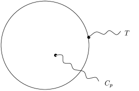
Figure 7.5: Disc amplitude for the two point function of the open string tachyon and the $p$-form R-R potential in the presence of a single non-BPS D$p$-brane. The aim of the computation is to establish the term Eq. (7.2.4) in the non-BPS D$p$-brane action.

This will establish the first term in the expansion of Eq. (7.2.2). We take the R-R vertex operator in the ($-1/2,-1/2$) picture (which exhibits the R-R field strengths rather than the potentials):

$$V_{\rm RR} = c(z)\tilde{c}(\bar{z})e^{-\phi(z)/2}e^{-\tilde{\phi}(\bar{z})/2}H_{\alpha\dot{\beta}}\,S^{\alpha}(z)\,\bar{S}^{\dot{\beta}}(\bar{z})\,e^{{\rm i}k\cdot X(z,\bar{z})}$$

$$\rightarrow c(z)c(\bar{z})e^{-\phi(z)/2}e^{-\phi(\bar{z})/2}H_{\alpha\dot{\beta}}\,S^{\alpha}(z)\,(\gamma^{0}\gamma^{1}\cdots\gamma^{p})^{\dot{\beta}}{}_{\dot{\gamma}}\,S^{\dot{\gamma}}(\bar{z})$$

$$e^{{\rm i}k\cdot X(z)}\,e^{{\rm i}k\cdot S\cdot X(\bar{z})}\leavevmode\nobreak\ ,$$

where $H_{\alpha\dot{\beta}}$ is the bispinor containing the R-R field strengths and $k$ the momentum of the R-R potential. We do not keep track of the overall normalization, since we are not able to directly determine the constant $a$ in Eq. (7.2.2) anyway. The tachyon vertex operator is put in the $-1$ picture:

$$V_{T}=c(y)e^{-\phi(y)}T(k^{\prime})\,e^{{\rm i}k^{\prime}\cdot X(y)}\leavevmode\nobreak\ \leavevmode\nobreak\ ,$$ (7.2.18)

where $T$ and $k^{\prime}$ are the tachyon polarization and momentum and $y$ is a point on the real axis. The three insertion points $z$, $\bar{z}$ and $y$ have been fixed by introducing ghost fields. The contributions of the ghost, superghost and $X$ sectors combine into $(z-\bar{z})^{5/4}$. The contraction of the two spin fields in the fermionic sector gives

$$<S^{\alpha}(z)\,S^{\dot{\gamma}}(\bar{z})>=(z-\bar{z})^{-5/4}\,C^{\alpha\dot{\gamma}}\leavevmode\nobreak\ \leavevmode\nobreak\ ,$$ (7.2.19)

with $C$ the charge conjugation matrix. Thus, the amplitude becomes

$$T\,H_{\alpha\dot{\beta}}(\gamma^{0}\gamma^{1}\cdots\gamma^{p})^{\dot{\beta}}{}_{\dot{\gamma}}\,C^{\alpha\dot{\gamma}}\times K\leavevmode\nobreak\ \leavevmode\nobreak\ ,$$ (7.2.20)

where $K$ is a global factor. Tracing over the spinor indices, only the part of $H_{\alpha\dot{\beta}}$ proportional to $H_{\mu_{1}\ldots\mu_{p+1}}(C\gamma^{\mu_{1}\ldots\mu_{p+1}})_{\alpha\dot{\beta}}$ contributes, making the amplitude proportional to $T\,H_{\mu_{1}\ldots\mu_{p+1}}\epsilon^{\mu_{1}\ldots\mu_{p+1}}$. Upon integration by parts, this confirms the first term of Eq. (7.2.2).

There is a kinematical subtlety in this computation. String scattering amplitudes can only be computed for on-shell external particles. It is easy to convince oneself that, since the tachyon carries only momentum along the brane and the momentum along the brane is conserved, the tachyon and the R-R potential cannot be both on-shell. As a way out, one could consider branes with Euclidean signature, for which this kinematical problem does not occur, and then extrapolate the couplings one finds there to their Minkowski cousins. The situation is analogous to the one we commented on in footnote 16 on page 16.

To check the second term of Eq. (7.2.2), depending linearly on $F$, we add to the previous amplitude a vertex operator for a gauge field (see Fig. 7.6).

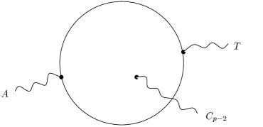
Figure 7.6: Disc amplitude for the three point function of the open string tachyon, the ($p-2$)-form R-R potential and the Born-Infeld gauge field in the presence of a single non-BPS D$p$-brane.

This vertex operator is in the 0 picture:

$$V_{A}=A_{\mu}({\rm i}\dot{X}^{\mu}(w)+2\alpha^{\prime}\,p\cdot\psi\psi^{\mu}(w))\,e^{{\rm i}p\cdot X(w)}\leavevmode\nobreak\ \leavevmode\nobreak\ ,$$ (7.2.21)

where this time we have kept track of all normalization factors. Here, $A_{\mu}$ is the polarization of the gauge field, $p$ is its momentum and $w$ is on the real axis. Only the fermionic part of the photon vertex operator can lead to terms of the type we are looking for (the photon should provide two gamma-matrices). We compute that part of the amplitude to lowest order in the photon momentum. This means that we will put $p$ equal to zero in the bosonic sector, thus keeping only the explicit $p$ dotted with a $\psi$ in Eq. (7.2.21). We follow the previous computation as closely as possible by fixing again $z$, $\bar{z}$ and $y$, such that only $w$ needs to be integrated over. In the limit of small photon momentum, the ghost, superghost and $X$ sector contributions are unchanged (they multiply to $(z-\bar{z})^{5/4}$). The fermionic correlator is

$$2\alpha^{\prime}p_{\nu}A_{\mu}<S^{\alpha}(z)\psi^{\nu}\psi^{\mu}(w)S^{\dot{\gamma}}(\bar{z})>=-{\rm i}\alpha^{\prime}p_{\nu}A_{\mu}(\gamma^{\nu\mu})^{\alpha\dot{\gamma}}(w-z)^{-1}(w-\bar{z})^{-1}(z-\bar{z})^{-1/4}.$$ (7.2.22)

The resulting integral can be done by a contour integration:

$$(z-\bar{z})\int_{-\infty}^{+\infty}\,dw\,(w-z)^{-1}(w-\bar{z})^{-1}=2\pi{\rm i}\leavevmode\nobreak\ \leavevmode\nobreak\ ,$$ (7.2.23)

leading to

$$2\pi\alpha^{\prime}\,p_{\nu}\,A_{\mu}\,T\,H_{\alpha\dot{\beta}}\,(\gamma^{\nu\mu})^{\alpha\dot{\gamma}}(\gamma^{0}\gamma^{1}\cdots\gamma^{p})^{\dot{\beta}}{}_{\dot{\gamma}}\,\times K$$ (7.2.24)

for the amplitude. This corresponds indeed to the term in Eq. (7.2.2) linear in $F$. Note that the factor $2\pi\alpha^{\prime}$ multiplying $F$ in Eq. (7.2.2) comes out correctly.

The generalization to multiple (low-momentum) photon insertions is straightforward. The dependence on the photon insertion points of the relevant part of the fermionic correlator factorizes, such that each integration reduces to the one-dimensional integral in Eq. (7.2.23). One can also include Chan-Paton factors in the computations, leading to the trace in Eq. (7.2.2). Finally, one could check the presence of the gravitational terms in Eq. (7.2.2) explicitly. Since all graviton vertex operators can be inserted in the ($0,0$) picture, the various contractions will be identical to the ones used in [7, 12, 8].

Note that, from a technical point of view, the only role of the tachyon in the above computations is to provide its superghost part, allowing one to insert the R-R vertex operator in the $(-1/2,-1/2)$ picture, instead of the ($-3/2,-1/2$) picture. Thus, the inclusion of the tachyon proves wrong one’s first impression that non-BPS D-branes cannot couple to the closed string R-R sector because of the GSO-projection. Apart from this, the above computations perfectly parallel their counterparts for BPS D-branes.

We mention some of the related developments in the recent literature. First, a Wess-Zumino action for brane–anti-brane pairs has been given in [116]. Second, it has been checked [117, 118] that the Wess-Zumino action Eq. (7.2.2) for non-BPS D-branes in type II string theory is consistent with T-duality, at least if the curvature terms are neglected. Third, this Wess-Zumino action has been supplemented with a Born-Infeld action [119, 120, 117, 118]. Finally, in [121], the non-BPS D-branes in type II string theory have been associated to non-trivial loops in the configuration space of type II string theory.

To summarize Chapter 7, we have introduced non-BPS D-branes as kink solutions of the tachyon field on a coincident D-brane–anti-D-brane pair. We have indicated how non-BPS D-branes play a role in checking string dualities and how D-brane charges are related to K-theory. The main result in this chapter is that non-BPS D-branes in type II string theory couple to R-R fields via the Wess-Zumino action Eq. (7.2.2) [11]. This action explains how vortex solutions of the tachyon field on the non-BPS D-brane, which were conjectured to correspond to BPS D-branes [100], acquire R-R charge. We have checked the action Eq. (7.2.2) by explicit string computations.

Appendix A Samenvatting

A.1 Snaartheorie

Een goede fysische theorie verklaart vele experimentele waarnemingen op een consistente manier vanuit een klein aantal fundamentele principes.

De algemene relativiteitstheorie is hiervan een voorbeeld. Haar principe is dat gravitatie veroorzaakt wordt door kromming van de ruimte-tijd. Ze verklaart diverse fenomenen, gaande van de zwaartekracht op de aarde tot planetenbewegingen en de afbuiging van licht door de zon. Een ander voorbeeld van een goede fysische theorie is het standaardmodel van de elementaire-deeltjesfysica. Het fundamentele principe is dat ijksymmetrieën aan de basis liggen van de elektromagnetische en kernkrachten. Vele voorspellingen van het standaardmodel zijn bevestigd in experimenten in deeltjesversnellers, soms met een verbazingwekkende precisie.

We hebben gezien dat de algemene relativiteitstheorie een goede theorie is voor de gravitationele interactie, terwijl het standaardmodel een goede beschrijving geeft van de sterke, zwakke en elektromagnetische interacties. Krijgen we een goede theorie van de vier fundamentele wisselwerkingen door de algemene relativiteitstheorie en het standaardmodel te combineren? Het probleem is dat de algemene relativiteitstheorie een klassieke theorie is, terwijl het standaardmodel een kwantumtheorie is. Samen geven ze geen consistente beschrijving van de natuur. Men zou kunnen proberen de algemene relativiteitstheorie te kwantiseren, maar alle rechtstreekse pogingen om dat te doen zijn mislukt.

Nochtans bestaat er een consistente kwantumtheorie die gravitatie beschrijft. Ze was ‘per ongeluk’ ontdekt op het einde van de jaren zestig en in het begin van de jaren zeventig, toen mensen een theorie voor de sterke interacties aan het zoeken waren. Pogingen om bepaalde experimentele waarnemingen over sterk interagerende deeltjes te begrijpen leidden tot het idee dat de sterke interacties door een theorie van snaren zouden kunnen worden beschreven. De populariteit van dit idee daalde toen bleek dat een andere theorie, kwantumchromodynamica (‘quantum chromodynamics’, QCD), de sterke interacties goed beschreef. Dit betekende echter niet het einde van snaartheorie: men had ontdekt dat snaartheorie onder andere een massaloos spin-2 deeltje beschrijft. Zo’n deeltje verwachtte men als drager van de gravitationele interactie in een kwantumtheorie van gravitatie!

Geïnspireerd door het feit dat ze gravitatie bevat, opperde men het idee dat snaartheorie alle interacties zou kunnen verenigen. Inderdaad ontdekte men dat snaartheorie ook de ijksymmetrieën van het standaardmodel bevat. Bijgevolg verenigt snaartheorie gravitatie en de ijksymmetrieën van het standaardmodel op consistente wijze! Consistentie alleen maakt snaartheorie echter nog geen goede fysische theorie. Daarvoor is het ook nodig dat de theorie vele experimentele waarnemingen verklaart uitgaande van een klein aantal fundamentele principes.

Wat de experimentele waarnemingen betreft, de eerste vereiste is dat snaartheorie de voorspellingen van de algemene relativiteitstheorie en het standaardmodel reproduceert, tenminste wanneer de omstandigheden zodanig zijn dat men weet dat deze theorieën een goede beschrijving van de natuur geven. Snaarfenomenologie is de tak van snaartheorie die zich bezighoudt met het zoeken naar zo’n snaarmodellen. De huidige situatie is dat het standaardmodel (nog) niet exact gereproduceerd is, maar dat er wel ‘semi-realistische’ modellen bestaan die aardig in de buurt komen.

Wat de fundamentele principes van snaartheorie betreft, een aantal hiervan moet vermoedelijk nog ontdekt worden. Nochtans zijn er verschillende aanwijzingen over de structuur van de theorie.

Ten eerste is het duidelijk dat de structuur van perturbatieve snaartheorie veel beperkender is dan die van kwantumveldentheorie: terwijl men in kwantumveldentheorie veel verschillende interacties kan bedenken, laat perturbatieve snaartheorie enkel het splitsen en samenkomen van snaren toe. Een volledige, niet-perturbatieve beschrijving van snaartheorie ontbreekt echter nog. Wat we weten is dat snaartheorie niet enkel een theorie van snaren is: ze bevat ook uitgebreide (d.w.z. meerdimensionale) objecten, ‘branen’ genoemd (de naam is een veralgemening van ‘membranen’). Het is niet duidelijk of de volledige theorie kan worden geformuleerd als een theorie van snaren.

Ten tweede speelt supersymmetrie, een symmetrie tussen bosonen en fermionen, een belangrijke rol in snaartheorie. Supersymmetrie zou een van de organiserende principes van snaartheorie kunnen zijn. Dat neemt niet weg dat er recent pogingen geweest zijn om betekenis te geven aan niet-supersymmetrische snaartheorieën.

Ten slotte zijn dualiteiten prominent aanwezig in de huidige ontwikkelingen in snaartheorie. Ze bieden de mogelijkheid aspecten van niet-perturbatieve snaartheorie te exploreren.

Tot nog toe hebben we snaartheorie besproken als mogelijke Theorie Van Alles. Snaartheorie kan echter ook op een andere manier een omwenteling teweegbrengen in ons begrip van de natuur: we kunnen snaartheorie gebruiken als hulpmiddel om iets te leren over kwantumveldentheorie, in het bijzonder over de ijktheorieën van het standaardmodel. Er is bijvoorbeeld hoop dat snaartheorie van nut kan zijn om het berucht sterke-koppelingsprobleem van QCD op te lossen. Hierop gaan we nu iets dieper in.

Kwantumchromodynamica (QCD) is een theorie van de sterke interacties. Ze behoort tot het standaardmodel. Bij hoge energie is de theorie zwak gekoppeld, zodat storingstheorie ons in staat stelt voorspellingen te doen voor verstrooiingsamplituden bij hoge energie. Die voorspellingen komen overeen met de experimentele resultaten. Bij lage energie is de theorie echter sterk gekoppeld, zodat storingstheorie nutteloos is. Het is niet bekend hoe berekeningen kunnen worden gedaan in dit regime. Nochtans zijn zulke berekeningen nodig om fenomenen als de opsluiting van quarks te begrijpen.

Onlangs is het vermoeden gerezen dat de sterke-koppelingslimiet van bepaalde veldentheorieën kan worden beschreven door een zwak gekoppelde duale snaartheorie [2]. Dit verband heet de AdS/CFT correspondentie. In zijn huidige vorm is het vermoeden niet echt van toepassing op QCD, maar het idee dat gerelateerde theorieën door specifieke snaartheorieën kunnen worden beschreven vertoont intrigerende gelijkenissen met de oorspronkelijke sterke-interactie motivatie voor snaartheorie!

A.2 D-branen

A.2.1 Algemeenheden

In de meeste recente ontwikkelingen in snaartheorie spelen D-branen een cruciale rol. D-branen maakten hun intrede in snaartheorie als hypervlakken waarop open strings kunnen eindigen. Het is echter duidelijk geworden dat ze dynamische objecten zijn: ze kunnen bewegen en hun vorm veranderen. D-branen vormen een bepaalde klasse van de uitgebreide objecten die we vermeldden in Sectie A.1, toen we zeiden dat snaartheorie niet enkel een theorie van snaren is. Wat D-branen onderscheidt van andere uitgebreide objecten is dat ze, hoewel ze zelf geen perturbatieve snaartoestanden zijn, een beschrijving hebben in perturbatieve snaartheorie: de dynamica van een D-braan wordt beschreven door de open snaren die erop eindigen. Dankzij deze eigenschap zijn D-branen veel makkelijker te bestuderen dan andere uitgebreide objecten in snaartheorie. D-branen zijn om de volgende redenen van belang.

Ten eerste duiken ze op in vele modellen van snaarfenomenologie. De hoofdreden is dat er ijkvelden op hun wereld-volume leven, in het bijzonder niet-abelse ijkvelden als verscheidene D-branen samenvallen. Deze ijkvelden kunnen de rol spelen van de ijkvelden van het standaardmodel. Van bijzonder belang voor fenomenologische doeleinden is de observatie dat D-branen kunnen zorgen voor het breken van supersymmetrie. Bijvoorbeeld zijn systemen met D-branen en anti-D-branen onlangs gebruikt om semi-realistische modellen te construeren [3].

Ten tweede zijn ze nadrukkelijk aanwezig in snaardualiteiten. Vaak corresponderen D-branen in de ene perturbatieve beschrijving van snaartheorie met fundamentele snaren in een duale beschrijving. In die zin zijn D-branen even fundamenteel als snaren.

Ten derde zijn D-branen gerelateerd met (meerdimensionale) zwarte gaten. In feite leveren D-branen en sommige zwarte gaten complementaire beschrijvingen van hetzelfde object. Welke beschrijving aangewezen is, hangt af van de koppelingsconstante van de snaartheorie. Deze correspondentie kan aangewend worden om het aantal toestanden te tellen van supersymmetrische (BPS) zwarte gaten. Voor zulke zwarte gaten verandert het aantal toestanden niet wanneer we de koppelingsconstante wijzigen, zodat hun toestanden evengoed kunnen worden geteld in het regime waar de beschrijving als D-braan geldig is. Deze procedure heeft geleid tot een microscopische verklaring voor de entropie van zwarte gaten, tenminste voor bepaalde supersymmetrische zwarte gaten.

Ten vierde liggen D-branen aan de basis van de AdS/CFT correspondentie, zoals blijkt uit Secties 5.1.1 and 6.1.

A.2.2 Aspecten bestudeerd in deze thesis

Nu we het belang van D-branen in snaartheorie aangetoond hebben, gaan we in op de concrete aspecten die in deze thesis bestudeerd worden.

Het grootste deel van de thesis is gewijd aan D-branen. In het bijzonder zijn we geïnteresseerd in de D-braan effectieve actie. Dat is een lage-energie effectieve actie voor de massaloze excitaties van het D-braan, d.w.z. voor de massaloze modes van de open snaren die de dynamica van het braan beschrijven. Men kan zich voorstellen dat men alle massieve modes van de open snaren ‘uitgeïntegreerd’ heeft. Het hoeft geen betoog dat zo’n effectieve, ‘macroscopische’ beschrijving handiger is voor berekeningen dan de volledige, ‘microscopische’ beschrijving in termen van open snaren.

Onze werkwijze om termen van de D-braan effectieve actie te berekenen bestaat erin verstrooiingsamplituden van snaren in de aanwezigheid van een D-braan te berekenen in de ‘microscopische’ snaartheorie. Dan leggen we op dat, tenminste bij lage energie, die amplituden gereproduceerd worden in de effectieve beschrijving. Het formalisme dat we gebruiken om de meeste van die amplituden te berekenen in snaartheorie is het randtoestand (‘boundary state’) formalisme. In dat formalisme wordt een D-braan voorgesteld als een bron van gesloten-snaartoestanden.

De termen in de D-braan actie waarin we vooral geïnteresseerd zijn, worden anomale koppelingen genoemd. Zij maken deel uit van de D-braan Wess-Zumino actie. Via het ‘anomalie instroom mechanisme’ zorgen ze ervoor dat de ijk- en gravitationele anomalieën in bepaalde configuraties van D-branen gecompenseerd worden. Op die manier zijn ze belangrijk voor de beroemde consistentie van snaartheorie. Onze belangrijkste bijdrage in dat kader bestaat in het expliciet nagaan van de aanwezigheid van de anomale koppelingen in de D-braan actie. Als een bonus vinden we extra termen in de D-braan actie. Deze extra termen zijn nieuw.

We breiden het anomalie instroom argument en de verstrooiingsberekeningen uit naar D-branen in de niet-supersymmetrische type 0 snaartheorieën. We leiden een Wess-Zumino actie af die opmerkelijk sterk lijkt op die voor D-branen in de supersymmetrische type II snaartheorieën. Zulke gelijkenissen tussen supersymmetrische en niet-supersymmetrische situaties in snaartheorie vormen een belangrijk thema in deze thesis. De type 0 D-branen zijn gebruikt om de AdS/CFT correspondentie uit te breiden naar niet-supersymmetrische veldentheorieën. We zetten onze studie van type 0 snaartheorieën verder door het spectrum af te leiden van NS-vijfbranen, andere uitgebreide objecten in die theorieën. We combineren onze kennis van D-branen en NS-vijfbranen om een recent dualiteitsvoorstel te becommentariëren.

Om een niet-supersymmetrische D-braan veldentheorie te bekomen, hoeft men niet van een niet-supersymmetrische snaartheorie te vertrekken. Men kan ook niet-supersymmetrische (niet-BPS) configuraties van D-branen beschouwen in een supersymmetrische snaartheorie. Zulke configuraties kunnen bijvoorbeeld bestaan uit BPS D-branen en hun anti-branen. Men kan ook niet-BPS D-branen beschouwen. Dat zijn onstabiele objecten in type II snaartheorie. Wij bestuderen die niet-BPS D-branen en leiden er een Wess-Zumino actie voor af. Die actie legt gedeeltelijk uit dat BPS D-branen overeenkomen met monopool-achtige configuraties in de wereld-volume theorie van niet-BPS D-branen.

Ten slotte gebruiken we de effectieve actie van BPS D-branen in type II snaartheorie om D-branen in de achtergrond van andere D-branen te bestuderen. Zulke configuraties hebben vele toepassingen. Wij concentreren ons op een toepassing in de AdS/CFT correspondentie, namelijk het analogon in snaartheorie van een extern baryon in veldentheorie.

We hebben ervoor gekozen onze aandacht in deze thesis bijna uitsluitend toe te spitsen op gesloten-snaartheorieën in tien vlakke, niet-compacte dimensies. Dat houdt in dat we een aantal gerelateerde onderwerpen waarover we gepubliceerd hebben, niet behandelen. In het bijzonder besteden we geen aandacht aan speciale Kählermeetkunde [6], anomale koppelingen van oriëntifold-vlakken [7, 8], de studie van D-branen in D-braan achtergronden via superalgebra’s [9], niet-supersymmetrische ijktheorieën afkomstig van type 0 orbifolds [10] en het randtoestand formalisme voor orbifolds [10]. We verwijzen geïnteresseerde lezers naar onze artikels over die onderwerpen.

Tot besluit, de voornaamste methoden die we gebruiken om D-branen te bestuderen, zijn het berekenen van verstrooiingsamplituden en het gebruik van consistentie-argumenten. We berekenen de meeste van die verstrooiingsamplituden in het randtoestand formalisme. De consistentie-argumenten houden verband met de compensatie van ijk- en gravitationele anomalieën via het mechanisme van anomalie instroom. We zijn geïnteresseerd in niet-supersymmetrische D-braan configuraties. In het bijzonder proberen we delen van de mooie structuur van supersymmetrische snaren en D-branen uit te breiden naar niet-supersymmetrische situaties.

A.3 Overzicht en samenvatting van de resultaten

In Sectie A.2.2 hebben we een kort overzicht gegeven van de onderwerpen die in deze thesis aan bod komen. Daarbij hebben we onze motivatie en methoden benadrukt. In deze sectie schetsen we de structuur van de thesis en geven we een iets meer gedetailleerde samenvatting van de resultaten.

De meeste van de resultaten zijn gepubliceerd in de artikels [7, 8, 9, 10, 11, 15]. Het is onze bedoeling ze in deze thesis op een coherente manier te presenteren en voldoende achtergrondmateriaal te voorzien om ze toegankelijk(er) te maken voor niet-specialisten. In het bijzonder denken we aan mensen die vertrouwd zijn met kwantumveldentheorie maar geen gedetailleerde kennis bezitten van deze tak van snaartheorie.

Enerzijds introduceren we in Hoofdstuk 2 een aantal sleutelbegrippen in een niet-snaartheoretische context, in het bijzonder in kwantumveldentheorie. Die begrippen zijn dualiteit, supersymmetrie en anomalie instroom. Anderzijds proberen we in Hoofdstuk 3 en Sectie 4.1 genoeg technische informatie over snaren, D-branen en randtoestanden aan te reiken opdat gemotiveerde lezers in staat zouden zijn de berekeningen in Hoofdstuk 4 te begrijpen, in het bijzonder die in Sectie 4.3, die meer in detail gegeven worden. Hoofstuk 3 is ook een noodzakelijke voorbereiding voor Hoofdstukken 5, 6 en 7. In wat volgt geven we voor de verschillende hoofdstukken een overzicht en een samenvatting van de resultaten.

A.3.1 Hoofdstuk 2: Enkele sleutelbegrippen

In Hoofdstuk 2 introduceren we drie sleutelbegrippen, meestal in een veldentheoretische context. In Sectie 2.1 geven we verscheidene voorbeelden van dualiteiten. We concentreren ons vooral op elektromagnetische dualiteit, in het bijzonder op de dualiteitsconjectuur van Montonen en Olive [33] en enkele raadsels die daarmee verbonden waren. In Sectie 2.2 tonen we hoe die raadsels op een natuurlijke wijze opgelost worden in supersymmetrische veldentheorie. We introduceren de supersymmetrie-algebra en het begrip ‘BPS toestand’. In Sectie 2.3 presenteren we enkele resultaten uit de literatuur over anomalieën en anomalie instroom. We concentreren ons op één voorbeeld [21, 22], waar men het instroom mechanisme expliciet aan het werk ziet. Omdat het anomalie instroom mechanisme een cruciaal begrip is in deze thesis, gaan we er nu kort op in.

Bij anomalie instroom kan men zich het volgende voorstellen [21, 22]. Beschouw een ijkveld dat op een niet-chirale manier aan fermionen gekoppeld is, laat ons zeggen in een vier-dimensionale ruimte-tijd. Bij gebrek aan chirale ijk-koppelingen, zal de ijksymmetrie niet-anomaal zijn. Veronderstel nu dat de fermionen bovendien op een chirale manier koppelen aan een scalair veld. Voor bepaalde configuraties van het scalaire veld is het mogelijk dat bepaalde fermion modes effectief op een lager-dimensionaal ‘defect’ van de ruimte-tijd leven, bijvoorbeeld op een twee-dimensionaal oppervlak. Als zulke fermion modes chiraal zijn in twee dimensies, kunnen ze een ijkanomalie veroorzaken in hun effectieve twee-dimensionale theorie. Dat kan op het eerste gezicht in tegenspraak lijken met het feit dat we vertrokken waren van een vierdimensionale theorie zonder chirale ijk-koppelingen.

De oplossing is dat de anomale variatie van de effectieve twee-dimensionale actie gecompenseerd wordt door een ijkvariatie veroorzaakt door de overblijvende fermion modes, die in de ‘bulk’ van de ruimte-tijd leven. Er is dus ‘anomalie instroom’ van de vier-dimensionale ruimte-tijd naar het twee-dimensionale ‘defect’. In meer fysische termen kan met het als volgt stellen. Kijkt men enkel naar de vrijheidgraden die effectief op het ‘defect’ leven, dan lijkt het alsof er (voor bepaalde achtergrondconfiguraties) ‘uit het niets’ lading gecreëerd wordt op het defect. Kijkt men echter ook naar de vrijheidsgraden in de ‘bulk’, dan merkt men dat die lading in werkelijkheid gewoon vanuit de ‘bulk’ naar het defect stroomt, en dat lading in de volledige theorie behouden is.

We zien hier dus dat, wanneer men de chirale vrijheidsgraden op het ‘defect’ kent, men bepaalde voorspellingen kan doen over de ‘bulk’ theorie. In het eenvoudige voorbeeld dat we besproken hebben, kan het lijken dat we hieruit niets leren wat we nog niet wisten. Het instroom mechanisme is echter een krachtig hulpmiddel in meer ingewikkelde situaties, zoals die welke we bespreken in Secties 3.5, 6.3.1 en 6.4.2.

A.3.2 Hoofdstuk 3: Snaren en branen

In Hoofdstuk 3 voeren we supersnaren en D-branen in. We doen een inspanning om op een coherente manier de begrippen in te voeren die relevant zijn voor deze thesis, in het bijzonder voor de berekeningen in Hoofdstuk 4.

In Sectie 3.1.1 voeren we snaren in vertrekkend van hun wereld-oppervlak beschrijving. We bestuderen onder andere het verschil tussen open en gesloten snaren, de verschillende sectoren (bijvoorbeeld R en NS voor open snaren), de spectra van snaarexcitaties en de GSO-projectie. We bespreken ook enkele meer technische aspecten, zoals spoken en BRST-kwantisatie. Deze technische aspecten zijn uiteraard van belang, maar om het grootste deel van onze expliciete berekeningen te volgen, is het niet nodig ze te kennen. De lezer kan er dus voor kiezen alles over spoken en BRST-operatoren over te slaan. In Sectie 3.1.2 bespreken we de lage-energie effectieve beschrijving van snaartheorie als een supergravitatietheorie in een tien-dimensionale ruimte-tijd. De wisselwerking tussen de wereld-oppervlak- en ruimte-tijd-beschrijvingen van snaartheorie is een van de hoofdthema’s in deze thesis. Sectie 3.2 gaat over supersnaren in achtergrondvelden.

In Sectie 3.3 verzamelen we een aantal hulpmiddelen om verstrooiingsamplituden te berekenen in snaartheorie. We introduceren het belangrijke begrip ‘vertex-operator’. Een groot deel van deze sectie is gewijd an technische aspecten, zoals (super)spoken, beelden (‘pictures’) en BRST-invariantie. Deze aspecten kunnen weer overgeslagen worden door lezers die er niet bijzonder in geïnteresseerd zijn. Ze zijn vooral nodig om onze latere keuzes van vertex-operatoren te rechtvaardigen. In Sectie 3.3.6 geven we een aantal van die vertex-operatoren.

In Sectie 3.4 introduceren we D-branen en hun effectieve actie. In het bijzonder tonen we een aantal anomale termen van de D-braan Wess-Zumino actie

$$S_{\rm WZ}=\frac{T_{p}}{\kappa}\int_{p+1}C\wedge e^{2\pi\alpha^{\prime}\,F+B}\wedge\sqrt{\hat{A}(R_{T})/\hat{A}(R_{N})}$$ (1)

in detail. De inhoud van deze sectie is van cruciaal belang om de thesis te begrijpen. Sectie 3.5 gaat over het anomalie instroom argument in de context van D-branen en NS-vijfbranen. We geven weinig technische details, maar de ideeën nemen een centrale plaats in in de thesis. Bijvoorbeeld zullen we anomalie instroom argumenten gebruiken in Secties 6.3.1 en 6.4.2. In Sectie 3.6 bestuderen we drie dualiteiten in snaartheorie. De discussie van type IIB S-dualiteit is nuttig als voorbereiding op Sectie 6.5, waar we een veralgemening ervan kritisch bestuderen.

A.3.3 Hoofdstuk 4: Anomale koppelingen uit snaarberekeningen

In dit hoofdstuk gaan we de aanwezigheid na van sommige van de anomale D-braan koppelingen in (3.4.9). Dat doen we door verstrooiingsamplituden van gesloten-snaartoestanden in de aanwezigheid van een D-braan expliciet te berekenen in snaartheorie. Daartoe gebruiken we het randtoestand formalisme. In Sectie 4.1 voeren we de randtoestand in en geven we een verzameling preciese regels over hoe hij moet worden gebruikt in verstrooiingsamplituden met een sfeer als wereld-oppervlak. Deze sectie bevat niet veel origineel werk, al is, voor zover wij weten, onze verzameling regels niet in de literatuur te vinden.

In Sectie 4.2 geven we een overzicht van de tests waaraan de Wess-Zumino actie (3.4.9) onderworpen is. Het blijkt dat er onrechtstreekse argumenten zijn voor de aanwezigheid van alle termen in (3.4.9), maar dat voor de termen met NS-NS velden alle rechtstreekse tests ontbraken tot ons artikel [7] verscheen. De indirecte argumenten gebruiken expliciet de consistentie van snaartheorie, in het bijzonder de afwezigheid van ijk- en gravitationele anomalieën. Directe tests van (3.4.9) gaan dus na of snaartheorie met D-branen inderdaad een consistente theorie is.

In Sectie 4.3 testen we de aanwezigheid van de term

$$\frac{T_{p}}{\kappa}\int_{p+1}\hat{C}_{p-1}\wedge\hat{B}$$ (2)

in de D-braan Wess-Zumino actie. Dankzij het voorbereidende werk in Hoofdstuk 3 en Sectie 4.1 kunnen we de berekeningen in detail tonen. We vinden de gezochte term inderdaad. Sectie 4.3 is een uitgebreide versie van een hoofdstuk van ons artikel [7].

In Sectie 4.4 bevestigen we de aanwezigheid (met de juiste coëfficiënt) van de termen

$$\frac{T_{p}}{\kappa}\int_{p+1}\hat{C}_{p-3}\wedge\frac{(4\pi^{2}\alpha^{\prime})^{2}}{384\pi^{2}}({\rm tr\,}R_{T}^{2}-{\rm tr\,}R_{N}^{2})\leavevmode\nobreak\ ,$$ (3)

waarin viervormen geconstrueerd uit krommings-tweevormen een rol spelen. Deze berekeningen werden eerst uitgevoerd in onze artikels [7, 8].

In Sectie 4.5, die gebaseerd is op ons artikel [8], beschouwen we de termen

$$\frac{T_{p}}{\kappa}\int_{p+1}\hat{C}_{p-7}\wedge\left(\frac{(4\pi^{2}\alpha^{\prime})^{4}}{294912\pi^{4}}({\rm tr\,}R_{T}^{2}-{\rm tr\,}R_{N}^{2})^{2}+\frac{(4\pi^{2}\alpha^{\prime})^{4}}{184320\pi^{4}}({\rm tr\,}R_{T}^{4}-{\rm tr\,}R_{N}^{4})\right)\leavevmode\nobreak\ .$$ (4)

Hierin staat een achtvorm opgebouwd uit krommings-tweevormen. Gebruik makend van de resultaten van [12], kunnen we de aanwezigheid van al deze termen bevestigen, inclusief de coëfficiënten. Bovendien vinden we, als bonus, extra D-braan koppelingen [8]. Die extra koppelingen, die nieuw zijn, zijn niet-anomaal, wat meteen verklaart waarom ze niet eerder gevonden waren door anomalie instroom argumenten.

A.3.4 Hoofdstuk 5: Baryon vertex in AdS/CFT

In dit hoofdstuk bespreken we een toepassing van de effectieve D-braan actie: we tonen hoe ze gebruikt kan worden om snaren eindigend op D-branen in D-braan achtergronden te bestuderen. We beschouwen onder andere een D5-braan gewikkeld rond de vijf-sfeer $S^{5}$ van een $AdS_{5}\times S^{5}$ ruimte. $AdS_{5}\times S^{5}$ is de structuur van de ruimte-tijd dichtbij de horizon van D3-branen. We zijn dus een D5-braan in de ‘near-horizon’ meetkunde van D3-branen aan het bestuderen. Deze configuratie speelt een rol in de AdS/CFT correspondentie [2]: een D5-braan gewikkeld rond $S^{5}$ is het analogon in snaartheorie van een baryon in de corresponderende veldentheorie [71].

In Sectie 5.1 geven we een korte inleiding tot de AdS/CFT correspondentie, de baryon vertex en de methode die we gebruiken om die baryon vertex te bestuderen: de BPS methode. Het vervolg van Hoofdstuk 5 is gebaseerd op ons artikel [9]. In Sectie 5.2 leggen we de BPS methode uit in een iets eenvoudigere situatie dan die welke ons zal interesseren. In Sectie 5.3 bestuderen we de baryon vertex configuratie en een gerelateerde configuratie in ons formalisme. We reproduceren de BPS-vergelijking (5.3.27) van [13, 14]. Een mooi aspect van onze methode is dat we resultaten kunnen afleiden die nauw verbonden zijn met supersymmetrie, en dit zonder expliciet fermionen te beschouwen. Een ander voordeel van onze methode is dat ze de mogelijkheid opent de BPS-vergelijking te herinterpreteren in termen van superalgebra’s [9]. In deze thesis bespreken we die herinterpretatie echter niet.

A.3.5 Hoofdstuk 6: Type 0 snaartheorie

Dit hoofdstuk is gewijd aan type 0 snaartheorie. Vergeleken met type II snaren hebben type 0 snaren een tachyon, dubbel zoveel R-R velden en geen ruimte-tijd fermionen in hun perturbatieve spectrum. De tachyonische fluctuatie signaleert dat we rond een onstabiel ‘vacuum’ aan het expanderen zijn. Wegens de problemen die de aanwezigheid van zo’n tachyonische mode met zich meebrengt, werden type 0 snaartheorieën pas anderhalf jaar geleden populair. Toen werd opgemerkt [83, 84] dat het tachyon niet noodzakelijk een probleem hoeft te zijn wanneer men, zoals in de AdS/CFT correspondentie, de effectieve veldentheorieën op het wereld-volume van D-branen wil bestuderen.

In Sectie 6.1 bespreken we deze motivatie om type 0 snaartheorie te bestuderen. Type 0 snaren worden geïntroduceerd in Sectie 6.2. In Sectie 6.3 voeren we type 0 D-branen in. Zoals kon worden verwacht op basis van het verdubbelde het R-R spectrum van type 0 snaren ten opzichte van type II snaren, zijn er ook tweemaal zoveel verschillende D-branen in type 0. Zoals in ons artikel [10] leiden we de Wess-Zumino actie (6.3.6) af voor type 0 D-branen:

$$S_{\rm WZ}=\frac{T_{p}}{\kappa}\int_{p+1}(C)_{\pm}\wedge{\rm e}^{2\pi\alpha^{\prime}\,F+B}\wedge\sqrt{\hat{A}(R_{T})/\hat{A}(R_{N})}\leavevmode\nobreak\ .$$ (5)

De $\pm$ geeft het verschil aan tussen ‘elektrische’ and ‘magnetische’ branen. Om deze actie af te leiden, maken we gebruik van een anomalie instroom argument. De aanwezigheid van de verschillende termen kan ook rechtstreeks getest worden zoals we deden voor type II D-branen.

We merken op dat niet alleen de Wess-Zumino actie voor type 0 D-branen zelf, maar ook de argumenten waarmee ze afgeleid en getest werd, zeer sterk lijken op wat we kennen van de supersymmetrische type II D-branen. Hoewel van (ruimte-tijd) supersymmetrie geen sprake is voor type 0 D-branen, lijken ze in sommige opzichten dus sterk op supersymmetrische type II D-branen.

Sectie 6.4 is gebaseerd op ons artikel [15], waar we NS-vijfbranen in type 0 snaartheorieën bestuderen. We leiden hun massaloze spectra af en vinden dat die spectra niet-chiraal en puur bosonisch zijn voor zowel type 0A als type 0B. We stellen een speculatieve interpretatie van de type 0 NS-vijfbraan spectra voor in termen van ‘type 0 kleine snaren’.

In Sectie 6.4.2 hebben we gezien dat type IIA NS-vijfbranen een chiraal spectrum hebben. Dit chiraal spectrum geeft aanleiding tot een gravitationele anomalie, die gecompenseerd wordt door anomalie instroom van de ‘bulk’ van de ruimte-tijd naar het vijfbraan. We berekenen dat voor zowel type 0A als type 0B de analoge ‘bulk’ term afwezig is. Er is dus geen instroom van de bulk naar de vijfbranen, wat consistent is met onze bevinding dat die vijfbranen een niet-chiraal spectrum hebben en dus geen gravitationele anomalie [15].

In [85] zijn een aantal dualiteiten van type 0 snaartheorieën voorgesteld. Een ervan is S-dualiteit van type 0B snaartheorie. In Sectie 6.5 combineren we onze studies van type 0 D-branen en NS-vijfbranen om enkele vragen op te werpen over type 0B S-dualiteit.

A.3.6 Hoofdstuk 7: Niet-BPS branen

In dit hoofdstuk bestuderen we niet-BPS D-branen. Dat zijn objecten waarop open snaren kunnen eindigen, maar die geen supersymmetrie bewaren. In sommige snaartheorieën kunnen zulke objecten stabiel zijn, maar in tien-dimensionale type II snaartheorie zijn ze het niet. In Sectie 7.1 geven we aan hoe werk van Sen het onderzoek naar niet-BPS D-branen op gang bracht. Het belangrijkste resultaat van Hoofdstuk 7 staat in Sectie 7.2, die gebaseerd is op ons artikel [11]. Daar stellen we voor de onstabiele niet-BPS D-branen van type II snaartheorie de Wess-Zumino actie (7.2.2) voor [11]:

$$S^{\prime}_{\rm WZ}=a\int_{p+1}\hat{C}\wedge d\,\left\{{\rm tr\,}\,T\,e^{2\pi\alpha^{\prime}\,F}\right\}\wedge e^{\hat{B}}\wedge\sqrt{\hat{A}(R_{T})/\hat{A}(R_{N})}\leavevmode\nobreak\ ,$$ (6)

waar $T$ het tachyonveld is dat de instabiliteit van het niet-BPS D-braan signaleert. Enerzijds argumenteren we [11] dat die actie consistent is met de interpretatie [100] van BPS D-branen als topologisch niet-triviale tachyon-configuraties op een niet-BPS D-braan. Anderzijds testen we de aanwezigheid van de verschillende termen door expliciete berekeningen in snaartheorie [11].

A.3.7 Besluit

De meest opvallende resultaten in deze thesis zijn waarschijnlijk

• de bevestiging van de aanwezigheid van verschillende anomale termen in de D-braan Wess-Zumino actie door expliciete berekeningen in snaartheorie (Hoofdstuk 4),

• het vinden van nieuwe, niet-anomale termen in de D-braan Wess-Zumino actie (Sectie 4.5),

• het uitbreiden van de BPS-methode naar D-branen in D-braan achtergronden (Hoofdstuk 5),

• de Wess-Zumino actie (6.3.6) voor type 0 D-branen (Sectie 6.3.1),

• de type 0 NS-vijfbraan spectra (Sectie 6.4)

• en de Wess-Zumino actie (7.2.2) voor niet-BPS D-branen in type II snaartheorie (Hoofdstuk 7).

References

- [1]
- [2] J. Maldacena, The large limit of superconformal field theories and supergravity, Adv. Theor. Math. Phys. 2 (1998) 231, hep-th/9711200.
- [3] G. Aldazabal, L.E. Ibanez and F. Quevedo, Standard-like models with broken supersymmetry from type I string vacua, J. High Energy Phys. 01 (2000) 031, hep-th/9909172.
- [4] F. Denef, Low energy physics from type IIB string theory, K.U. Leuven Ph.D. thesis (1999).
- [5] A. Strominger and C. Vafa, Microscopic origin of the Bekenstein-Hawking entropy, Phys. Lett. B379 (1996) 99, hep-th/9601029.
- [6] B. Craps, F. Roose, W. Troost and A. Van Proeyen, Special Kähler geometry. Does there exist a prepotential?, in Strings, branes and dualities, NATO ASI series, L. Baulieu et al. eds., Kluwer Academic Publishers, 1999, p. 449, hep-th/9712092; What is special Kähler geometry? Nucl. Phys. B503 (1997) 565, hep-th/9703082; The definitions of special geometry, in Second international Sakharov conference on physics: Proceedings, I.M. Dremin and A.M. Semikhatov eds., World Scientific, 1997, p. 390, hep-th/9606073.
- [7] B. Craps and F. Roose, Anomalous D-brane and orientifold couplings from the boundary state, Phys. Lett. B445 (1998) 150, hep-th/9808074.
- [8] B. Craps and F. Roose, (Non-) Anomalous D-brane and O-plane couplings: the normal bundle, Phys. Lett. B450 (1999) 358, hep-th/9812149.
- [9] B. Craps, J. Gomis, D. Mateos and A. Van Proeyen, BPS solutions of a D5-brane worldvolume in a D3-brane background from superalgebras, J. High Energy Phys. 04 (1999) 004, hep-th/9901060.
- [10] M. Billó, B. Craps and F. Roose, On D-branes in type 0 string theory, Phys. Lett. B457 61-69, hep-th/9902196.
- [11] M. Billó, B. Craps and F. Roose, Ramond-Ramond couplings of non-BPS D-branes, J. High Energy Phys. 06 (1999) 033, hep-th/9905157.
- [12] B. Stefanski, Gravitational Couplings of D-branes and O-planes, Nucl. Phys. B548 (1999) 275, hep-th/9812088.
- [13] Y. Imamura, Supersymmetries and BPS configurations on anti-de Sitter space, Nucl. Phys. B537 (1999) 184, hep-th/9807179.
- [14] C.G. Callan, A. Güijosa and K.G. Savvidy, Baryons and string creation from the fivebrane worldvolume action, hep-th/9810092.
- [15] B. Craps and F. Roose, NS fivebranes in type 0 string theory, J. High Energy Phys. 10 (1999) 007, hep-th/9906179.
- [16] J. Harvey, Magnetic monopoles, duality, and supersymmetry, hep-th/9603086.
- [17] D. Olive, Exact electromagnetic duality, in Strings, branes and dualities, NATO ASI series, L. Baulieu et al. eds., Kluwer Academic Publishers, 1999, p. 3.
- [18] B. Zumino, Chiral anomalies and differential geometry, in Relativity, groups and topology II, proceedings of the Les Houches summer school, B.S. DeWitt and R. Stora eds., Elsevier Science Publishers B.V., 1984, p. 1291.
- [19] L. Alvarez-Gaumé and P. Ginsparg, The structure of gauge and gravitational anomalies, Ann. Phys. (NY) 161 (1985) 423.
- [20] W.A. Bardeen and B. Zumino, Consistent and covariant anomalies in gauge and gravitational theories, Nucl. Phys. B244 (1984) 421.
- [21] C.G. Callan and J.A. Harvey, Anomalies and fermion zero modes on strings and domain walls, Nucl. Phys. B250 (1985) 427.
- [22] S. Naculich, Axionic strings. Covariant anomalies and bosonization of chiral zero modes, Nucl. Phys. B296 (1988) 837.
- [23] H.A. Kramers and G.H. Wannier, Statistics of the two-dimensional ferromagnet, I and II, Phys. Rev. 60 (1941) 252, 263.
- [24] T.H.R. Skyrme, Particle states of a quantized meson field, Proc. Roy. Soc. A262 (1961) 237.
- [25] S. Coleman, Quantum sine-Gordon equation as the massive Thirring model, Phys. Rev. D11 (1975) 2088; S. Mandelstam, Soliton operators for the quantized sine-Gordon equation, Phys. Rev. D11 (1975) 3026.
- [26] P.A.M Dirac, Quantised singularities in the electromagnetic field, Proc. Roy. Soc. A33 (1931) 60.
- [27] D. Zwanziger, Quantum field theory of particles with both electric and magnetic charges, Phys. Rev. 176 (1968) 1489; J. Schwinger, A magnetic model of matter, Science 165 (1969) 757.
- [28] F. Englert and R. Brout, Broken symmetry and the mass of gauge vector bosons, Phys. Rev. Lett. 13 (1964) 321; P. Higgs, Spontaneous symmetry breakdown without massless bosons, Phys. Rev. 145 (1966) 1156; T.W.B. Kibble, Symmetry breaking in non-abelian gauge theories, Phys. Rev. 155 (1967) 1554.
- [29] G. ’t Hooft, Magnetic monopoles in unified gauge theories, Nucl. Phys. B79 (1974) 276; A.M. Polyakov, Particle spectrum in quantum field theory, JETP Lett. 20 (1974) 194.
- [30] E.B. Bogomol’nyi, The stability of classical solutions, Sov. J. Nucl. Phys. 24 (1976) 449.
- [31] M.K. Prasad and C.M. Sommerfield, Exact classical solution for the ’t Hooft monopole and the Julia-Zee dyon, Phys. Rev. Lett. 35 (1975) 760.
- [32] P. Goddard, J. Nuyts and D.I. Olive,Gauge theories and magnetic charge, Nucl. Phys. B125 (1977) 1.
- [33] C. Montonen and D.I. Olive, Magnetic monopoles as gauge particles?, Phys. Lett. B72 (1977) 117.
- [34] A. D’Adda, R. Horsley and P. Di Vecchia, Supersymmetric monopoles and dyons, Phys. Lett. B76 (1978) 298.
- [35] E. Witten and D. Olive, Supersymmetry algebras that include topological charges, Phys. Lett. B78 (1978) 97.
- [36] H. Osborn, Topological charges for supersymmetric gauge theories and monopoles of spin 1, Phys. Lett. B83 (1979) 321.
- [37] A. Sen, Dyon-monopole bound states, self-dual harmonic forms on the multi-monopole moduli space, and SL(2,) invariance in string theory, Phys. Lett. B329 (1994) 217, hep-th/9402032.
- [38] J. Polchinski, String theory, 2 volumes, Cambridge University Press, 1998.
- [39] M. Green, J. Schwarz and E. Witten, Superstring Theory, 2 volumes, Cambridge University Press, 1987.
- [40] D. Lüst and S. Theisen, Lectures on string theory, Springer-Verlag, Berlin, 1989.
- [41] E. Kiritsis, Introduction to superstring theory, Leuven University Press, 1998.
- [42] D. Friedan, E. Martinec and S. Shenker, Conformal invariance, supersymmetry and string theory, Nucl. Phys. B271 (1986) 93.
- [43] C. Bachas, Lectures on D-branes, hep-th/9806199.
- [44] M. Billó, P. Di Vecchia, M. Frau, A. Lerda, I. Pesando, R. Russo and S. Sciuto, Microscopic string analysis of the D0-D8 brane system and dual R-R states, Nucl. Phys. B526 (1998) 199, hep-th/9802088.
- [45] P. Di Vecchia, M. Frau, I. Pesando, S. Sciuto, A. Lerda, R. Russo, Classical -branes from boundary state, Nucl. Phys. B507 (1997) 259, hep-th/9707068.
- [46] C.P. Bachas, P. Bain and M.B. Green, Curvature terms in D-brane actions and their M-theory origin, J. High Energy Phys. 05 (1999) 011, hep-th/9903210.
- [47] J. Polchinski, Dirichlet branes and Ramond-Ramond charges, Phys. Rev. Lett. 75 (1995) 4724, hep-th/9510017.
- [48] F. Denef, A. Sevrin and J. Troost, Non-abelian Born-Infeld versus string theory, hep-th/0002180.
- [49] R.C. Myers, Dielectric-branes, J. High Energy Phys. 12 (1999) 022, hep-th/9910053.
- [50] M. Green, J. Harvey and G. Moore, I-brane inflow and anomalous couplings on D-branes, Class. Quant. Grav. 14 (1997) 47, hep-th/9605033.
- [51] Y.-K. Cheung and Z. Yin, Anomalies, branes, and currents, Nucl. Phys. B517 (1998) 69, hep-th/9710206.
- [52] C.G. Callan, J.A. Harvey and A. Strominger, Worldbrane actions for string solitons, Nucl. Phys. B367 (1991) 60.
- [53] M.J. Duff, J.T. Liu and R. Minasian, Eleven dimensional origin of string/string duality: a one loop test, Nucl. Phys. B452 (1995) 261, hep-th/9506126; E. Witten, Five-branes and M-theory on an orbifold, Nucl. Phys. B463 (1996) 383, hep-th/9512219.
- [54] C. Vafa and E. Witten, A one-loop test of string duality, Nucl. Phys. B447 (1995) 261, hep-th/9505053.
- [55] C. Callan, C. Lovelace, C. Nappi and S. Yost, Adding holes and crosscaps to the superstring, Nucl. Phys. B293 (1987) 83.
- [56] C. Lovelace, Phys. Lett. B34 (1971) 500; L. Clavelli and J. Shapiro, Nucl. Phys. B57 (1973) 490; M. Ademollo, R. D’Auria, F. Gliozzi, E. Napolitano, S. Sciuto and P. di Vecchia, Nucl. Phys. B94 (1975) 221.
- [57] M. Frau, I. Pesando, S. Sciuto, A. Lerda and R. Russo, Scattering of Closed Strings from Many D-branes, Phys. Lett. B400 (1997) 52, hep-th/9702037.
- [58] M.B. Green and N. Seiberg, Contact interactions in superstring theory, Nucl. Phys. B299 (1987) 599.
- [59] M. Gutperle, Contact terms, symmetries and D-instantons, Nucl. Phys. B508 (1997) 133, hep-th/9705023.
- [60] M. Li, Boundary states of D-branes and Dy-strings, Nucl. Phys. B460 (1996) 351.
- [61] M.R. Douglas, Branes within branes, in Strings, branes and dualities, NATO ASI series, L. Baulieu et al. eds., Kluwer Academic Publishers, 1999, p. 267, hep-th/9512077.
- [62] M. Bershadsky, V. Sadov and C. Vafa, D-branes and topological field theories, Nucl. Phys. B463 (1996) 420, hep-th/9511222.
- [63] J. Morales, C. Scrucca and M. Serone, Anomalous couplings for D-branes and O-planes, Nucl. Phys. B552 (1999) 291, hep-th/9812071.
- [64] O. Aharony, S.S. Gubser, J. Maldacena, H. Ooguri and Y. Oz, Large field theories, string theory and gravity, hep-th/9905111.
- [65] E. Witten, AdS/CFT correspondence and topological field theory, J. High Energy Phys. 12 (1998) 012, hep-th/9812012.
- [66] G.T Horowitz and A. Strominger, Black strings and p-branes, Nucl. Phys. B360 (1991) 197.
- [67] E. Witten, Anti-de Sitter space and holography, Adv. Theor. Math. Phys. 2 (1998) 253, hep-th/9802150.
- [68] S.S. Gubser, I.R. Klebanov and A.M. Polyakov, Gauge theory correlators from non-critical string theory, Phys. Lett. B428 (1998) 105, hep-th/9802109.
- [69] J.M. Maldacena, Wilson loops in large N field theories, Phys. Rev. Lett. 80 (1998) 4859, hep-th/9803002.
- [70] S.-J. Rey and J. Yee, Macroscopic strings as heavy quarks of large N gauge theory and anti-de Sitter supergravity, hep-th/9803001.
- [71] E. Witten, Baryons and branes in anti de Sitter space, J. High Energy Phys. 07 (1998) 006, hep-th/9805112.
- [72] C.G. Callan and J.M. Maldacena, Brane dynamics from the Born-Infeld action, Nucl. Phys. B513 (1998) 198-212, hep-th/9708147.
- [73] G.W. Gibbons, Born-Infeld particles and Dirichlet p-branes, Nucl. Phys. B514 (1998) 603, hep-th/9709027.
- [74] J.P. Gauntlett, J. Gomis and P.K. Townsend, Bogomolnyi bounds for worldvolume solitons, J. High Energy Phys. 01 (1998) 033, hep-th/9711205.
- [75] E. Bergshoeff, J. Gomis and P.K. Townsend, M-brane intersections from worldvolume superalgebras, Phys. Lett. B421 (1998) 109, hep-th/9711043.
- [76] A. Hanany and E. Witten, Type IIB superstrings, BPS monopoles and three-dimensional gauge dynamics, Nucl. Phys. B492 (1997) 152, hep-th/9611230.
- [77] E. Bergshoeff, G. Papadopoulos and J.P. van der Schaar, Domain walls on the brane, Phys. Lett. B430 (1998) 63, hep-th/9801158.
- [78] J.M. Camino, A.V. Ramallo, J.M. Sanchez de Santos, Worldvolume dynamics of D-branes in a D-brane background, Nucl. Phys. B562 (1999) 103, hep-th/9905118.
- [79] U. Danielsson, G. Ferretti and I. Klebanov, Creation of fundamental strings by crossing D-branes, Phys. Rev. Lett. 79 (1997) 1984, hep-th/9705084; O. Bergman, M.R. Gaberdiel and G. Lifschytz, Branes, orientifolds and the creation of elementary strings, Nucl. Phys. B509 (1998) 194, hep-th/9705130.
- [80] J. Gauntlett, N. Lambert and P. West, Supersymmetric fivebrane solitons, Adv. Theor. Math. Phys. 3 (1999) 91, hep-th/9811024.
- [81] J. Gomis, A. Ramallo, J. Simon and P. Townsend, Supersymmetric baryonic branes, J. High Energy Phys. 11 (1999) 019, hep-th/9907022.
- [82] L.J. Dixon and J.A. Harvey, String theories in ten dimensions without spacetime supersymmetry, Nucl. Phys. B274 (1986) 93.
- [83] A.M. Polyakov, The wall of the cave, Int. Jour. of Mod. Phys. A14 (1999) 645, hep-th/9809057.
- [84] I.R. Klebanov and A.A. Tseytlin, D-branes and dual gauge theories in type 0 strings, Nucl. Phys. B546 (1999) 155, hep-th/9811035.
- [85] O. Bergman and M.R. Gaberdiel, Dualities of type 0 strings, J. High Energy Phys. 07 (1999) 022, hep-th/9906055.
- [86] O. Bergman and M.R. Gaberdiel, A non-supersymmetric open string theory and S-duality, Nucl. Phys. B499 (1997) 183, hep-th/9701137.
- [87] J.A. Minahan, Glueball spectra and other issues for supergravity duals of QCD models, J. High Energy Phys. 01 (1999) 020, hep-th/9811156.
- [88] I.R. Klebanov and A.A. Tseytlin, Asymptotic freedom and infrared behavior in the type 0 string approach to gauge theory, Nucl. Phys. B547 (1999) 143, hep-th/9812089.
- [89] I.R. Klebanov and A.A. Tseytlin, A non-supersymmetric large N CFT from type 0 string theory, J. High Energy Phys. 03 (1999) 015, hep-th/9901101.
- [90] C.P. Bachas, M.R. Douglas and M.B. Green, Anomalous creation of branes, J. High Energy Phys. 07 (1997) 002, hep-th/9705074.
- [91] P.K. Townsend, M-theory from its superalgebra, in Strings, branes and dualities, NATO ASI series, L. Baulieu et al. eds., Kluwer Academic Publishers, 1999, p. 141, hep-th/9712004.
- [92] S.W. Hawking, Gravitational instantons, Phys. Lett. A60 (1977) 81.
- [93] D. Brill, Phys. Rev. B133 (1964) 845; C.N. Pope, Nucl. Phys. B141 (1978) 432; J.P. Gauntlett and D.A. Lowe, Dyons and S-duality in N=4 supersymmetric gauge theory, Nucl. Phys. B472 (1996) 194, hep-th/9601085.
- [94] N. Seiberg and E. Witten, Spin structures in string theory, Nucl. Phys. B276 (1986) 272.
- [95] N. Seiberg, New theories in six dimensions and matrix description of M-theory on T5 and T, Phys. Lett. B408 (1997) 98, hep-th/9705221.
- [96] A. Sen, Stable non-BPS states in string theory, J. High Energy Phys. 06 (1998) 007, hep-th/9803194.
- [97] A. Sen, Tachyon condensation on the brane antibrane system, J. High Energy Phys. 08 (1998) 012, hep-th/9805170.
- [98] A. Sen, SO(32) spinors of type I and other solitons on brane-antibrane pair, J. High Energy Phys. 09 (1998) 023, hep-th/9808141.
- [99] E. Witten, D-branes and K-theory, J. High Energy Phys. 12 (1998) 019, hep-th/9810188.
- [100] P. Horava, Type IIA D-branes, K-theory, and matrix theory, Adv. Theor. Math. Phys. 2 (1998) 1373, hep-th/9812135.
- [101] A. Sen, Non-BPS states and branes in string theory, hep-th/9904207.
- [102] A. Lerda and R. Russo, Stable non-BPS states in string theory: a pedagogical review, hep-th/9905006.
- [103] M. Atiyah, K-theory, W.A. Benjamin Inc., New York, 1967.
- [104] M. Karoubi, K-theory, an introduction, Springer-Verlag, Grundlehren der matematischen Wissenschaften 226, Berlin, 1978.
- [105] E. Witten, String theory dynamics in various dimensions, Nucl. Phys. B443 (1995) 85, hep-th/9503124.
- [106] J. Polchinski and E. Witten, Evidence for heterotic-type I string duality, Nucl. Phys. B460 (1996) 525, hep-th/9510169.
- [107] N. Berkovits, The tachyon potential in open Neveu-Schwarz string field theory, hep-th/0001084; N. Berkovits, A. Sen and B. Zwiebach, Tachyon condensation in superstring field theory, hep-th/0002211; P.-J. De Smet and J. Raeymaekers, Level four approximation to the tachyon potential in superstring field theory, hep-th/0003220.
- [108] A. Sen, Stable non-BPS bound states of BPS D-branes, J. High Energy Phys. 08 (1998) 010, hep-th/9805019.
- [109] O. Bergman and M.R. Gaberdiel, Stable non-BPS D-particles, Phys. Lett. B441 (1998) 133, hep-th/9806155.
- [110] O. Bergman and M.R. Gaberdiel, Non-BPS states in heterotic – type IIA duality, J. High Energy Phys. 03 (1999) 013, hep-th/9901014.
- [111] M. Frau, L. Gallot, A. Lerda and P. Strigazzi, Stable non-BPS D-branes in Type I string theory, Nucl. Phys. B564 (2000) 60, hep-th/9903123.
- [112] R. Minasian and G. Moore, K-theory and Ramond-Ramond charge, J. High Energy Phys. 11 (1997) 002, hep-th/9710230.
- [113] T. Eguchi, P.B. Gilkey and A.J. Hanson, Gravitation, gauge theories and differential geometry, Phys. Rep. 66 (1980) 213.
- [114] A. Sen, BPS D-branes on non-supersymmetric cycles, J. High Energy Phys. 12 (1998) 021, hep-th/9812031.
- [115] A. Hashimoto and I. Klebanov, Scattering of strings from D-branes, Nucl. Phys. Proc. Suppl. 55B (1997) 118, hep-th/9611214.
- [116] C. Kennedy and A. Wilkins, Ramond-Ramond couplings on brane-antibrane systems, Phys. Lett. B464 (1999) 206, hep-th/9905195.
- [117] K. Kamimura and J. Simon, T-duality covariance of superD-branes, hep-th/0003211.
- [118] E.A. Bergshoeff, M. de Roo, T.C. de Wit, E. Eyras and S. Panda, T-duality and actions for non-BPS D-branes, hep-th/0003221.
- [119] A. Sen, Supersymmetric world-volume action for non-BPS D-branes, J. High Energy Phys. 10 (1999) 008, hep-th/9909062.
- [120] M.R. Garousi, Tachyon couplings on non-BPS D-branes and Dirac-Born-Infeld action, hep-th/0003122.
- [121] J.A. Harvey, P. Horava and P. Kraus, D-sphalerons and the topology of string configuration space, J. High Energy Phys. 03 (2000) 021, hep-th/0001143.