UUITP-02/00

USITP-00-05

hep-th/0004187

D3-brane Holography

Ulf H. Danielsson,¹ Alberto Güijosa,²
Martín Kruczenski,¹ and Bo Sundborg²

¹ Institutionen för Teoretisk Fysik, Box 803, SE-751 08 Uppsala, Sweden

² Institute of Theoretical Physics, Box 6730, SE-113 85 Stockholm, Sweden

ulf@teorfys.uu.se, alberto@physto.se,
martink@teorfys.uu.se, bo@physto.se

Abstract

It has recently been conjectured that the AdS₅/SYM₄ correspondence can be generalized away from the conformal limit, to a duality between supergravity on the full asymptotically flat three-brane background and a theory characterized as ${\mathcal{N}}=4$ SYM deformed in the IR by a specific dimension-eight operator. Assuming that this relation is valid, we derive a prescription for computing $n$-point correlation functions in the holographic theory, which reduces to the standard AdS/CFT recipe at low energies. One- and two-point functions are discussed in detail. The prescription follows from very simple considerations and appears to be applicable to any asymptotically flat background. We also compute the quark-antiquark potential and comment on the description of the baryon in the supergravity picture. We conclude with some comments on the possible relation between our work and recent results in non-commutative field theories.

April 2000

1 Introduction

The path that led to the discovery of the AdS/CFT correspondence [1, 2, 3] began with the realization that the physics of D-branes can be captured from two quite distinct perspectives: as extended objects in supergravity, or as localized objects with intrinsic worldvolume dynamics [5]. Over the years, an enormous body of evidence has accumulated in support of this insight. In the particular case of D3-branes, the works [6, 7, 8, 9] performed a variety of comparisons between quantities in the two alternative descriptions, and constituted very important steps on our way to unraveling the precise relation between the two approaches. It was from these works that Maldacena [1] was able to distill his statement of equivalence between the extreme low-energy limit of the worldvolume dynamics (governed by ${\mathcal{N}}=4$ SYM in four dimensions) and type IIB string theory in the near-horizon region of the three-brane supergravity solution (i.e., $\mbox{AdS}_{5}\times{\mathbf{S}}^{5}$).

More recently, the authors of [10, 11, 12] have attempted to take another step along this path, by exploring the possibility of elevating the AdS/CFT correspondence to a duality between type IIB string theory defined on the full asymptotically flat three-brane background, and the effective theory describing the low-energy worldvolume dynamics of D3-branes at strong ’t Hooft coupling. The latter theory has been characterized in [11, 12] as an IR deformation of the ${\mathcal{N}}=4$ fixed point by a specific dimension-eight operator. To directly examine this non-renormalizable gauge theory would constitute an enormously difficult challenge. In this paper, we pursue a different line of attack. We assume that there exists a holographic image of physics on the D3 background, even if its precise form may be unknown to us. By definition, all information about this holographic dual is encoded in the bulk supergravity theory, since the duality mapping must work in both directions. Our approach will thus be to study the duality by developing a calculational procedure that extracts this information from the bulk theory.

The paper is structured as follows. In the next section we give a more detailed account of the proposal of [10, 11, 12], and delineate our approach. In Section 3 we derive a prescription for computing two-point correlators, using as a concrete example the operators that couple to dilaton partial waves. Section 4 contains a discussion of the two-point function we obtain, demonstrating that it reduces to the known ${\mathcal{N}}=4$ SYM result at low energies, and establishing its relation with the supergravity absorption probability. The result differs in some aspects from the one discussed by previous authors [10, 11]. In Section 5 we calculate a one-point function in the presence of an external source, and use it to discuss the UV/IR relation, encountering some interesting features. The prescription is then generalized to arbitrary $n$-point functions in Section 6. Sections 7 and 8 are respectively devoted to a calculation of the quark-antiquark potential and the description of baryons as D5-branes. A final section presents our conclusions, and includes some comments on the close parallel between certain aspects of our results and recent work in non-commutative field theories.

2 The Physics of D3-branes

In this section we will carefully examine the regimes of applicability of the two alternative descriptions of a system of D3-branes, and review the proposal of [10, 11, 12] for generalizing the AdS/CFT correspondence [1] to a duality involving the full D3-brane background. We should emphasize from the outset that, although our work was motivated by the existence of this relatively concrete duality conjecture, the route we choose to follow does not explicitly rely on its specific form. We will simply assume there exists some brane theory dual to supergravity on the three-brane background, and proceed in Sections 3 and onward to derive rules for computing quantities in the dual theory in terms of physics on the curved background.

2.1 Dual descriptions of D3-branes

Consider a collection of a large number, $N$, of D3-branes in Type IIB string theory. On the one hand, the physics of this system can be described in terms of a worldvolume theory coupled to string theory in the bulk of flat ten-dimensional spacetime. For processes with substringy energies, $\omega\ll m_{s}$, only the lowest modes of the D3-branes and the closed strings can be excited, and the description is in terms of a non-Abelian gauge theory coupled to supergravity. The action for the combined system is then

$$S=S_{\mathrm{S}}\left[\phi,h,\ldots\right]+S_{D3}\left[A,\Phi,\ldots;\phi,h\ldots\right]~{},$$ (1)

where the two terms denote the Type IIB supergravity action in a flat background and the D3-brane action, respectively. The degrees of freedom on the branes include a gauge field $A^{\mu}_{ab}$, six scalars $\Phi^{i}_{ab}$ ($a,b=1,\ldots,N$; $\mu=0,\ldots,3$; $i=4,\ldots,9$), and their fermionic superpartners. For discussion purposes it is convenient to split the D3-brane action into two terms, $S_{D3}=S_{\mathrm{b}}[A,\Phi,\ldots]+S_{\mathrm{int}}[A,\Phi,\ldots;\phi,h,\ldots]$, describing the dynamics on the brane and the couplings to the supergravity fields, respectively. The brane action $S_{b}$ includes in particular contributions from the Born-Infeld term, which are schematically of the form

$$S_{\mathrm{b}}=-N\int d^{4}x\,\mathop{\rm Tr}\left\{F^{2}+R^{4}F^{4}+\ldots\right\}~{}.$$ (2)

Note that the gauge field $A$, as well as the scalars $\Phi$ (not shown explicitly), have been ’t Hooft-normalized. This is the normalization which is most convenient in studying the large $N$ limit.

On the other hand, the system under consideration can be studied as a black brane solution of supergravity, with metric

$$ds^{2} = H^{-1/2}(-dt^{2}+dx_{1}^{2}+dx_{2}^{2}+dx_{3}^{2})+H^{1/2}(dr^{2}+r^{2}d\Omega_{5}^{2}),$$ (3)

$$H(r) = 1+{R^{4}\over r^{4}},\qquad R^{4}=4\pi Ng_{s}l_{s}^{4}~{},$$

a constant dilaton $e^{\bar{\phi}}=g_{s}~{}$, and $N$ units of Ramond-Ramond flux through the five-sphere. The above metric describes a geometry with an asymptotically flat region $r\geq R$, and a throat extending from $r=R$ down to a horizon at $r=0$. One can trust this supergravity solution as long as $R\gg l_{s}$, or in other words, $Ng_{s}\gg 1$.

Henceforth we will refer to the above two descriptions as the flat and the curved pictures, respectively. It should be emphasized that simultaneous validity of the two descriptions requires

$$\omega l_{s}\ll 1,\qquad R/l_{s}\gg 1,$$ (4)

but the combination $\omega R$ is arbitrary, as pointed out already in [7]. When this combination is small it represents a convenient expansion parameter.

That the curved and flat space pictures should be in some sense equivalent has been clear since Polchinski’s identification of D-branes as RR-charged black branes [5]. At the string level one has the option of either formulating the worldsheet theory as a non-linear $\sigma$-model for closed strings in the non-trivial three-brane background, or introducing explicit D3-branes by considering holes on the worldsheet with appropriate boundary conditions. We emphasize that in the latter description the spacetime metric one perturbs about is flat, the non-trivial geometry having being traded for the cumulative effect of open string loops.

Initial evidence for the equivalence of the two pictures came from the early D-brane scattering calculations [15]. A more systematic exploration of the precise connection between the two descriptions began with the comparison of thermodynamic quantities [6] and absorption cross-sections [7, 8, 9] computed in the two approaches.

Based partly on these works, Maldacena motivated his duality conjecture [1] by noting that in the low-energy limit, $\omega R\to 0$, the branes in the flat picture decouple from the bulk (i.e., $S_{\mathrm{int}}\to 0$). In addition, it can be seen from (2) that in this limit only the leading term survives, and the worldvolume theory reduces to ${\mathcal{N}}=4$ SYM. In taking the limit, the dimensionless ratio $\Phi/\omega$ should be held fixed. It is convenient and customary to regard $\omega$ as fixed and finite, in which case the low-energy decoupling is achieved by taking $R\to 0$.

The expectation value of the Higgs field is related to the radial coordinate in the curved picture through $r=R^{2}\Phi$. So if $R\to 0$ with $\Phi$ fixed, we have $r\propto R^{2}\to 0$, and as a result $H(r)\to(R/r)^{4}$, which means that we zoom in on the near-horizon geometry, AdS${}_{5}\times{\mathbf{S}}^{5}$. The gauge theory energy $\omega$ corresponds in the curved picture to the energy measured at infinity, and is related to the locally measured energy $\omega_{r}$ through $\omega=[H(r)]^{-1/4}\omega_{r}$. So even though $\omega R\to 0$, the fact that $r/R^{2}$ is held fixed implies that $\omega_{r}R$ stays fixed and finite, and consequently stringy excitations remain in the spectrum. Maldacena’s remarkable conclusion is that the full string theory in AdS${}_{5}\times{\mathbf{S}}^{5}$ can be equated with ${\mathcal{N}}=4$ SYM [1]. The string and SYM couplings are related through $g_{YM}^{2}=2\pi g_{s}$. For $g_{s}\ll 1$ and $g_{s}N\gg 1$ the bulk description is in terms of classical supergravity. Quantum $g_{s}$ and stringy $l_{s}/R$ corrections about this limit are mapped onto $1/N$ and $1/\lambda^{1/4}$ corrections in the gauge theory, respectively, where $\lambda=g_{YM}^{2}N$ is the ’t Hooft coupling.

Let us now try to obtain a holographic dual that describes more than just the near-horizon geometry. Such information would be included if we keep $\omega R$ finite [7, 10, 16]. It is clear from (2) that $S_{b}$ will then include terms of dimension higher than four. The worldvolume theory is thus no longer conformally invariant, its behaviour at different scales being described by a particular renormalization group trajectory. Just like in the AdS case, we expect a UV/IR correspondence [17, 18] to operate, relating the bulk radial coordinate $r$ to an energy scale in the field theory. The non-conformal nature of the worldvolume theory is thus simply a reflection of the fact that the supergravity background is no longer $SO(4,2)$-invariant, and as a result it has different properties at different values of $r$.

In accord with (4), we of course still restrict attention to substringy energies. But because we now work away from the extreme low-energy limit, the branes and the bulk do not decouple. As pointed out in [11], we can still achieve a decoupling of sorts in the weak coupling limit $g_{s}\to 0$. The flat space supergravity theory becomes free, and interactions can only take place on the worldvolume of the branes, with coupling strength $g_{s}N$. It is thus natural to conjecture that the physics in the full three-brane metric is dual to the worldvolume action for the D3-branes [7, 10, 16, 11].

Notice that, if we as usual wish to regard $\omega$ as being arbitrary, then to comply with (4) we must take $l_{s}\to 0$. To retain the non-conformal information we are then forced to simultaneously send $g_{s}N\to\infty$ in such a way that $R\sim(g_{s}N)^{1/4}l_{s}$ remains fixed. Even if we do not describe the limit this way, (4) requires that the theory on the branes be strongly coupled, $\lambda=g_{YM}^{2}N\gg 1$, in order for the curved picture supergravity background to be reliable. As emphasized in [11], this requirement implies that the worldvolume action cannot be merely the Born-Infeld action. The latter arises from a disk-level string calculation, so it does not incorporate the effects of summing over worldsheets with an arbitrary number of boundaries.

2.2 Explicit conjectures

To formulate an explicit duality conjecture, it is thus necessary to determine the low-energy effective action for a large number of D-branes at strong ’t Hooft coupling— undoubtedly a daunting task. Fortunately, as explained in [11, 12], string-theoretic information highly constrains the possible form of the required action. First of all, the theory must reduce to ${\mathcal{N}}=4$ SYM in the extreme infrared, corresponding to the fact that the three-brane metric reduces to AdS for $r\to 0$. For small but finite energy, the Lagrangian of the dual theory can be expressed as a deformation of the superconformal fixed point by irrelevant operators,

$${\mathcal{L}}={\mathcal{L}}_{SYM}+\sum_{d>4}h_{d}R^{d-4}{\mathcal{O}}_{d}~{},$$ (5)

where $d$ denotes the dimension of the non-renormalizable operator ${\mathcal{O}}_{d}$, and $h_{d}$ is a dimensionless coupling.

The irrelevant operators $\{{\mathcal{O}}_{d}\}$ ought to be compatible with the symmetries of the three-brane background: they must preserve sixteen supersymmetries (i.e., non-conformal ${\mathcal{N}}=4$) and be invariant under the $SO(6)\sim SU(4)$ R-symmetry. The least irrelevant such operator is

$${\mathcal{O}}_{8}=Q^{4}\bar{Q}^{4}\mathop{\rm Tr}\Phi^{4}=\mathop{\rm Tr}\left\{F^{4}-{1\over 4}(F^{2})^{2}+\ldots\right\}~{},$$ (6)

which happens to be the leading correction to SYM obtained by expanding the Born-Infeld action (see [22] and references therein). As indicated schematically in (6), ${\mathcal{O}}_{8}$ lies in a short multiplet of the ${\mathcal{N}}=4$ algebra: it is a supersymmetric descendant of the chiral primary operator $\mathop{\rm Tr}\Phi^{4}$ (where the product of scalar fields is understood to be symmetrized and traceless). ${\mathcal{O}}_{8}$ is dual to a supergravity field $\pi$ which has mass-squared $m^{2}=32/R^{2}$ and describes deformations of the trace of the AdS₅ and ${\mathbf{S}}^{5}$ metrics [23, 24, 25].

Now, the AdS/CFT correspondence predicts that for strong ’t Hooft coupling, all operators in the gauge theory except those in short multiplets acquire large anomalous dimensions, $d\sim\lambda^{1/4}$. For $\lambda\gg 1$, then, the sum in (5) is effectively restricted to run only over operators in short multiplets. All of the supergravity fields dual to such operators were tabulated in [23]. It is shown there that the aforementioned field $\pi$ is in fact the only scalar $SO(6)$-singlet mode with positive mass-squared (i.e., dual to an irrelevant gauge theory operator). Gubser and Hashimoto [11] were thus led to conjecture that, at least for $g_{s}\to 0$ and $g_{s}N\to\infty$, physics on the curved three-brane background is holographically encoded in the Lagrangian

$${\mathcal{L}}={\mathcal{L}}_{SYM}+h_{4}R^{4}{\mathcal{O}}_{8}~{}.$$ (7)

This was interpreted in [11] as a Wilsonian effective Lagrangian with a cutoff of order $R$.

To test their conjecture, Gubser and Hashimoto computed the absorption probability $P$ for arbitrary dilaton partial waves in the three-brane background, exploiting the remarkable fact that the relevant equation of motion has an exact solution in terms of associated Mathieu functions [11] (see also [26]). From $P$ it is possible to deduce, through an application of the optical theorem, the two-point correlator of the gauge theory operator dual to the dilaton partial wave under consideration. This exercise was carried out in [11] for the dilaton s-wave, employing the logic explained in [9, 27, 4]. In Section 4 we will demonstrate that the form of the optical theorem used in [11] is incomplete. Nevertheless, the two-point function which satisfies the correct optical theorem (and which follows directly from the prescription we will develop in the following section) has a form similar to the one presented in [11]. It was argued in [11] that this form could potentially be fully explained in terms of the Lagrangian (7), although of course a perturbative calculation would not be expected to reproduce the precise numerical coefficients obtained at strong coupling from the supergravity calculation. For the first correction to the conformal result, this comparison was carried out already in [10]. A closely related comparison can be found in [20, 21].

The conjecture of Gubser and Hashimoto was further analysed and considerably strengthened in subsequent work by Intriligator [12]. The last author arrived at (7) from a somewhat different perspective. His starting point is the assumption that there exists some four-dimensional theory dual to the background (3) with an arbitrary $SO(6)$-symmetric harmonic function

$$H(r)=h+{R^{4}\over r^{4}}~{}.$$ (8)

Intriligator then argues that the scaling properties of the metric imply that $h$ should be interpreted as a coupling constant which multiplies an operator in the dual theory whose dimension is exactly eight at all scales. As stated before, a renormalization group flow dual to the three-brane background must preserve sixteen supersymmetries. From a detailed analysis of flows with these many supersymmetries, the author of [12] concluded that along them the gauge coupling constant does not run, and the dimensions of operators in short multiplets remain constant. In the case of immediate interest, the former property is in line with the fact that the background dilaton is constant, while the latter property implies that ${\mathcal{O}}_{8}$ has dimension exactly eight along the entire flow. In this manner, Intriligator arrived at the conclusion that the background (3) with harmonic function (8) is holographically dual to the four-dimensional gauge theory whose Lagrangian is exactly (7) along the entire flow, with $h_{4}\sim h$ [12]. This duality statement includes the AdS₅/SYM₄ correspondence ($h=0$) as a particular case. The case $h=1$ is of course the full three-brane background, and all other cases with $h>0$ are related to this by a rescaling of $r$ and $x^{\mu}$. It was emphasized in [12] that the dimension-eight operator that enters the duality could potentially be a linear combination of the single-trace operator (6) and the double-trace operator $\mathop{\rm Tr}F^{2}\mathop{\rm Tr}F^{2}+\ldots$, which has exactly the same quantum numbers.

While the information reviewed so far indicates that ${\mathcal{O}}_{8}$ (possibly with some double-trace admixture) is the only short-multiplet operator of relevance for the duality, it does not yet rule out that long-multiplet $SU(4)$-symmetric operators preserving sixteen supersymmetries could appear in the deformed Lagrangian (5). If present, they would be important for the duality conjecture away from the strong-coupling regime. Intriligator argued that this is in fact not possible, because such operators would have to enter the Lagrangian multiplied by a $g_{YM}$-dependent power of $h$, and this would lead to a non-trivial running of the gauge coupling constant, in contradiction with the fact that the dilaton in the supergravity background is constant [12]. Intriligator has thus conjectured that (7) is in fact the exact holographic dual of type IIB string theory on the background (3) with harmonic function (8), for any value of $g_{s}$ and $N$. Notice that the duality has now been phrased in terms of the full string theory, as opposed to just supergravity: as explained before, if $g_{s}N$ and $\omega R$ are arbitrary, then $\omega l_{s}$ is also arbitrary, implying that it is possible to excite higher string modes. String excitations would in fact be present on both sides of the duality, so it is not clear if a sensible meaning can be ascribed to a duality statement involving only the gauge theory modes.

In a sense, the statement that (7) is dual to the full D3-brane geometry is a special case of the AdS₅/SYM₄ correspondence. Given that the operator ${\mathcal{O}}_{8}$ is dual to the supergravity field $\pi$, the deformation of ${\mathcal{L}}_{SYM}$ by ${\mathcal{O}}_{8}$ should describe a background which asymptotes to AdS space, with the mode $\pi$ excited.

The standard situation would be to consider ${\mathcal{N}}=4$ SYM as a UV fixed point, and perturb away from it by adding relevant operators ${\mathcal{O}}_{d}$, $d<4$ (see [4] and references therein). In that case the asymptotic $r\to\infty$ geometry is AdS, with the appropriate supergravity field excited and having a radial-dependence $r^{d-4}$. The dimension of the operator and the mass of the dual field are related through $d=2+\sqrt{4+m^{2}R^{2}}$ [2, 3].

On the contrary, for the deformation indicated in (7) one regards ${\mathcal{N}}=4$ SYM as an IR fixed point. The geometry is thus required to be asymptotically AdS as $r\to 0$. Expanding the metric (3) with harmonic function (8), one finds that to linear order in $h$

$$ds^{2}\simeq ds_{AdS}^{2}+{h\over 2}\left({r\over R}\right)^{4}\left[-\left({r\over R}\right)^{2}(-dt^{2}+{d\mathbf{x}}^{2})+\left({R\over r}\right)^{2}dr^{2}+R^{2}d\Omega_{5}^{2}\right]~{}.$$ (9)

The form of the perturbation, and in particular its dependence on $r^{4}$ (relative to AdS), is consistent with a deformation associated with the field $\pi$, whose mass satisfies $m^{2}R^{2}=32$ [33]. As $r$ increases, the metric perturbation indicated in (9) grows large, so it becomes necessary to solve the full non-linear supergravity equations. The complete solution is of course the three-brane background, which differs drastically from AdS at large $r$.

On the gauge theory side, we are attempting to define the theory starting from the IR fixed point and following the RG flow in the reverse direction. The presence of a non-renormalizable interaction would ordinarily point to the need for a new definition of the theory in the UV. On this issue, Intriligator espoused the view that (7) describes the theory at all scales, with the understanding that the coefficients of all other irrelevant operators are fine-tuned to zero [12].

We do not necessarily subscribe to this view. In particular, we should stress that, if D-branes are invoked to motivate the duality, then to us it seems inevitable that excited open string modes enter the duality at super-stringy energies, $\omega>m_{s}$. Such energies can certainly be reached if both $R$ and $g_{s}N$ are finite. On the other hand, Intriligator’s line of argument does not really equate the dual theory with the D3-brane worldvolume theory: the duality is asserted to hold for arbitrary $g_{s}$ and $N$, whereas we know that (7) certainly does not summarize the low-energy dynamics of a small number of weakly coupled branes, $g_{s}\ll 1$, $N\sim 1$. So whether or not it is correct, this strong form of the duality conjecture cannot be said to rest directly on D-brane intuition. Instead, it is based on the (by now fairly standard) assumption that any theory of gravity can be described holographically through a lower-dimensional non-gravitational theory [34, 35].

2.3 Our approach

Given the immense difficulties encountered in attempting a direct analysis of the candidate dual theory, we choose to follow an indirect route. We assume that there exists some theory which is the holographic image of physics on the three-brane background. We will henceforth refer to this theory as the ‘holographic dual’. Based on this existence assumption, in the following sections we will develop calculational tools that allow us to compute quantities in the holographic dual in terms of supergravity. The spirit of our approach is similar to that of [36, 37, 38], in that we use a conjectural duality to extract information about the dual theory. Since our calculations are based entirely on the supergravity side of the duality, our results contain information about whatever theory turns out to be the holographic dual of the D3-brane background, even if it is not of the form (7) along the entire RG flow. Notice in particular that the fact that the supergravity solution is smooth for all $r$ presumably indicates that the dual theory is sensible at all energy scales. We regard our work as a step towards a more precise specification of this dual theory.

3 Holographic Two-Point Function from Supergravity

If there exists a duality relating supergravity in a D3-brane background to some four-dimensional theory, the duality mapping ought to work in both directions. By definition, the lower-dimensional theory should holograph supergravity in the ten-dimensional background. Conversely, the physics of the holographic theory should be encoded in the bulk. In particular, a prescription should exist for computing correlation functions of the dual theory in terms of the curved D3 spacetime. In this section we will construct such a prescription. For definiteness, we focus on the two-point function of the operator dual to the dilaton s-wave. The extension to higher partial waves is straightforward; the main steps are described in Appendix B, and the final result is quoted at the end of this section. We will generalize the recipe to higher correlators in Section 6.

Before we proceed, we should take a moment to indicate why we have found it necessary to develop a new prescription. In the AdS/CFT case it has been argued [39, 40] that the GKPW recipe [2, 3] essentially equates correlation functions in the CFT with (generalized) AdS scattering amplitudes. It is thus natural to guess that the GKPW prescription can be carried over to our setting by simply replacing the AdS bulk-to-boundary propagator with the corresponding solution in the full D3 background. Unfortunately, this guess yields a two-point function which fails to reproduce the correct absorption probability, and suffers from severe problems at high energies. In this section, following a more physical approach, we will be arrive at a prescription which gives a two-point function in accord with the absorption results (see Section 4), and has a built-in subtraction and amputation procedure which automatically ensures a well-defined UV limit.

3.1 The prescription

Consider a dilaton propagating in the presence of $N$ D3-branes. Let us denote the corresponding propagator by $G(r,r^{\prime})$ (for the time being we focus only on the $r$-dependence; the other nine directions are left implicit). Viewing the branes as a supergravity solution, this propagator is obtained to lowest order in $g_{s}$ by solving the linearized equation of motion for the dilaton in the curved ten-dimensional background. Higher-order corrections, involving supergravity interactions, are suppressed in the $g_{s}\to 0$ limit. In taking this limit, we keep the geometry fixed, i.e., we hold $R^{4}\propto g_{s}N$ constant.

On the other hand, we can view the D-branes as (3+1)-dimensional objects with intrinsic dynamics, embedded in a flat (9+1)-dimensional ambient spacetime. In the obvious coordinate system, they are localized (along six directions) at $r=0$. The $l$th partial wave of the canonically normalized dilaton $\phi$ couples with unit strength to an operator in the worldvolume theory which will be denoted by ${\mathcal{O}}_{\phi}$ (the angular-momentum labels of these operators will be left implicit). The leading low-energy terms of these operators can be found in [41]. The dilaton s-wave, in particular, couples to the operator

$${\mathcal{O}}_{\phi}=-{\sqrt{2\pi}\over 4}\mathop{\rm Tr}\left\{(\sqrt{2}\pi R^{2})^{2}F^{2}+(\sqrt{2}\pi R^{2})^{4}\left(F^{4}-{1\over 4}(F^{2})^{2}\right)+\ldots\right\}~{},$$ (10)

where the ‘$\ldots$’ represent scalar and fermion dimension-four operators present already in the conformal limit [41], as well as additional operators of dimension eight and possibly higher which are corrections away from this limit [10]. We remind the reader that the field strength $F$ in (10) is ’t Hooft-normalized, i.e., the combination which appears in the worldvolume action is $N\mathop{\rm Tr}F^{2}$.

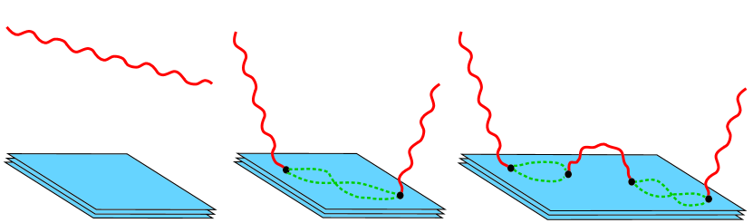
Figure 1: Propagation of a flat space dilaton in the presence of D3-branes. Starting from point $r$, the dilaton can reach $r^{\prime}$ a) directly, or b,c) indirectly, after having interacted with the branes. Black dots denote insertions of the operator ${\mathcal{O}}_{\phi}$, and dotted lines represent worldvolume processes.

A dilaton can propagate from $r$ to $r^{\prime}$ either directly (Fig. 1a), or indirectly, after having interacted with the branes (e.g., as depicted in Figs. 1b,c) by means of the coupling $\int d^{4}x\,\phi{\mathcal{O}}_{\phi}$. This results in a series of contributions to the propagator which are expressed diagrammatically in Fig. 2, where $C_{n}$ denotes the ‘pure worldvolume’ connected $n$-point correlator of ${\mathcal{O}}_{\phi}$ (i.e., the correlator computed exclusively with the brane action $S_{b}$ described in Section 2).

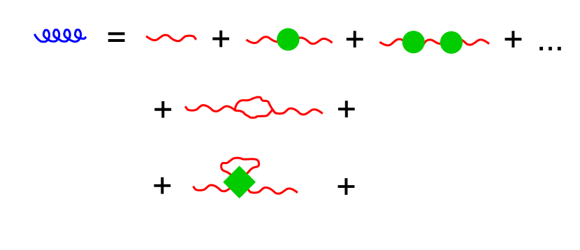
Figure 2: Diagrammatic expansion for the two-point dilaton correlator. The full propagator $G$ is written out in terms of the flat space propagator $G_{0}$, flat space supergravity vertices, and ‘pure-brane’ $n$-point correlators $C_{n}$. The first three diagrams on the right-hand side correspond to processes of the type shown in Figs. 1a, 1b and 1c, respectively. See text for discussion.

If we take the ‘decoupling’ limit $g_{s}\to 0$ with the ’t Hooft coupling $\lambda\propto g_{s}N$ fixed, the expansion in Fig. 2 simplifies drastically. Diagrams involving supergravity vertices evidently vanish. In addition, almost all diagrams involving brane correlation functions drop out. The $g_{s}$-dependence of the correlators is known in the conformal limit, from the standard AdS/CFT correspondence. According to the GKPW recipe [2, 3], boundary theory correlators are obtained from bulk AdS diagrams with $n$ external dilaton legs which terminate at the boundary. $C_{2}$ is consequently $g_{s}$-independent, since the relevant graph is just the propagator. The graphs for (connected) higher-order correlators feature supergravity vertices, and as a result, (the leading large-$N$ contribution to) $C_{n}$ is proportional to $g_{s}^{n-2}$. From the point of view of the field theory, this corresponds to the large-$N$ factorization of correlation functions. It is thus clear that in the $g_{s}\to 0$ limit, the expansion in Fig. 2 collapses to

$$G(r,r^{\prime}) = G_{0}(r,r^{\prime})+G_{0}(r,0)C_{2}G_{0}(0,r^{\prime})+G_{0}(r,0)C_{2}G_{0}(0,0)C_{2}G_{0}(0,r^{\prime})+\ldots$$ (11)

$$= G_{0}(r,r^{\prime})+G_{0}(r,0)\Delta_{2}G_{0}(0,r^{\prime}),$$

where $G_{0}$ is the flat-space dilaton propagator, and in the second line we have denoted by $\Delta_{2}$ the sum of the indicated series.

It might seem surprising that even at vanishing $g_{s}$ the branes are capable of emitting and reabsorbing dilatons. From the string theory perspective, diagrams with additional closed strings usually have extra handles, and are thus suppressed as $g_{s}\to 0$. However, what looks like an extra handle in going from, e.g., Fig. 1b to Fig. 1c, in fact sews together two surfaces which would otherwise be disjoint. The net effect is to add some number of boundaries to the original surface. In this manner, each successive term in the first line of (11) originates from a string diagram with additional worldsheet boundaries, which contribute additional powers of $g_{s}N$, not of $g_{s}$. Since we work in the regime of strong ’t Hooft coupling, the entire series in (11) must indeed be kept. Notice this means that there is no way to disentangle processes like those shown in Fig. 1c from the ‘purely worldvolume’ graphs that are contained in $C_{2}$. String theory thus dictates that it is $\Delta_{2}$, and not $C_{2}$, which must be regarded as the two-point correlator of ${\mathcal{O}}_{\phi}$,

$$\Delta_{2}=\langle{\mathcal{O}}_{\phi}\,{\mathcal{O}}_{\phi}\rangle~{},$$ (12)

in the effective theory summarizing the dynamics of the ‘decoupled’ brane system. This is the theory which can be expected to holograph the physics of the curved D3 background.

If we identify $G(r,r^{\prime})$ in (11) with the curved space dilaton propagator, then the equality can a priori only be expected to hold in the limit $r,r^{\prime}\to\infty$, because it is only far away from the branes that one can meaningfully compare $G$ with the flat space propagator $G_{0}$. The essential point here is that, if we took (11) as it stands as our definition of $\Delta_{2}$, then we would expect $\Delta_{2}$ to depend on $r,r^{\prime}$, complicating its interpretation as a correlator in a four-dimensional theory. Our main goal in the remainder of this section and the next will be to show that, on the contrary,

$$\Delta_{2}=\lim_{r,r^{\prime}\to\infty}\frac{G(r,r^{\prime})-G_{0}(r,r^{\prime})}{G_{0}(r,0)G_{0}(0,r^{\prime})}$$ (13)

is a well-defined quantity which can be rightfully interpreted as the desired four-dimensional holographic correlator.

3.2 Calculation of the correlator

To examine the limit $r,r^{\prime}\to\infty$, we first need to discuss the propagators in more detail. In order for the essential points to be more easily appreciated, we will first carry out the calculations at a general level, postponing explicit evaluations to the next subsection. The propagators $G$ and $G_{0}$ are defined as solutions to the ten-dimensional dilaton equation of motion

$$\partial_{M}\left[\sqrt{-g}\,g^{MN}\partial_{N}G\right]=\delta^{(10)}(X-X^{\prime})$$ (14)

in the respective backgrounds. Upon projecting onto a plane wave $\exp(ik_{\mu}x^{\mu})$ for the directions parallel to the three-branes, and onto the constant mode on ${\mathbf{S}}^{5}$, one is left with an equation for the radial propagator $G(k^{\mu};r,r^{\prime})$ of the form

$$\left\{\partial_{r}^{2}+{\partial_{r}f\over f(r)}\partial_{r}+{V_{k}(r)}\right\}G={\delta(r-r^{\prime})\over\pi^{3}f(r)},$$ (15)

where $f(r)=\sqrt{-g}g^{rr}$. Since we regard $G(k;r,r^{\prime})$ as the field created at $r$ by a source at $r^{\prime}$, it must satisfy boundary conditions such that (for $\omega\equiv k^{0}>0$) the associated flux moves away from the source.

At $r\not=r^{\prime}$, (15) is just the homogeneous equation for radial motion of the dilaton. Denote the solution with the required behaviour at $r\to 0$ (and consequently at all $r<r^{\prime}$) by $\phi_{1}$. Similarly, let $\phi_{2}$ be the solution of the homogeneous equation obeying the appropriate boundary condition at $r\to\infty$. Finally, take $\phi_{3}$ to be the solution which is linearly independent from $\phi_{2}$ and satisfies the ‘opposite’ boundary condition at $r\to\infty$. Of course, the solutions $\{\phi_{1},\phi_{2},\phi_{3}\}$ are not independent, and we can write

$$\phi_{1}=A\phi_{3}+B\phi_{2}~{},$$ (16)

with $A,B$ some overlap coefficients. It is clear that the $r$-dependence of the propagator can be expressed in the form

$$G(r,r^{\prime})=\left\{{{\alpha(r^{\prime})\phi_{1}(r)\quad\mbox{if}\quad r<r^{\prime}}\atop{\beta(r^{\prime})\phi_{2}(r)\quad\mbox{if}\quad r>r^{\prime}}}\right.$$ (17)

for some $\alpha,\beta$. These functions of $r^{\prime}$ can be determined by demanding that the propagator be continuous at $r=r^{\prime}$, and its first derivative have a discontinuity at $r=r^{\prime}$ which yields the delta-function in (15), with unit coefficient. The end result is

$$G(r,r^{\prime})={1\over w_{32}A}\phi_{2}(r_{>})\phi_{1}(r_{<})={1\over w_{32}}\phi_{2}(r_{>})\left[\phi_{3}(r_{<})+{B\over A}\phi_{2}(r_{<})\right],$$ (18)

where $r_{<}$ ($r_{>}$) is the smaller (larger) of $r$ and $r^{\prime}$, $w_{32}$ is the constant appearing in the Wronskian $W_{32}(r)=\phi_{3}\partial_{r}\phi_{2}-\phi_{2}\partial_{r}\phi_{3}=w_{32}/f(r)$, and $A,B$ are the overlap coefficients defined in (16).

Now we have enough information to explore the nature of the limit in (13). By definition, the flat space solution $\phi_{02}$ ($\phi_{03}$) must asymptote to a purely outgoing (ingoing) wave as $r\to\infty$: $\phi_{02}(r)\to r^{-5/2}\exp[i(qr+\theta_{0})]$. This must be true as well for the corresponding solution in the asymptotically flat D3 background, with the same $q$ but a different ‘phase shift’, $\theta$. Finally, the flat space solution $\phi_{01}$ must be regular at the origin, which implies that $A_{0}=B_{0}$, and $G_{0}(r,0)\to r^{-5/2}\exp[i(qr+\theta_{0})]$. Using all of this in (13) one is left with

$$\Delta_{2}={1\over w_{32}}\left[{w_{012}\over\phi_{01}(0)}\right]^{2}\Bigg{[}{B\over A}e^{2i(\theta-\theta_{0})}-1\Bigg{]}~{},$$ (19)

where $A,B$ are the curved space overlap coefficients and $w_{012}/f(r)$ is the Wronskian of the indicated flat-space solutions. As advertised, all $r,r^{\prime}$-dependence cancels out, and the limit is well-defined. This result is as expected from our derivation of (13), and serves as a first consistency check on our approach.

3.3 Explicit evaluation

Having explained the essential points, let us now proceed to the explicit determination of the dilaton propagators. Using the metric (3) in (14), the curved space propagator $G(k^{\mu};r,r^{\prime})$ can easily be seen to satisfy (15) with $f(r)=r^{5}$ and $V_{k}(r)=q^{2}H(r)$, where we have defined $q^{2}=\omega^{2}-\vec{k}^{2}$. As explained in [11] (see also [26]), the corresponding homogeneous equation can be related to Mathieu’s equation, and the solutions of interest to us are found to be

$$\phi_{1}(r) = r^{-2}H^{(1)}(\nu,-\ln(r/R))~{},$$

$$\phi_{2}(r) = r^{-2}H^{(1)}(\nu,+\ln(r/R))~{},$$

$$\phi_{3}(r) = r^{-2}H^{(2)}(\nu,+\ln(r/R))~{}.$$ (20)

Unless otherwise noted, we adopt the notation of [11]: $H^{(1,2)}(\nu,z)$ are associated Mathieu functions of the third and fourth kind, respectively, and $\nu$ is the ‘Floquet exponent’ (an $l$-dependent function of $qR$) defined in [11, 26]. In line with the previous discussion, the following boundary conditions have been enforced: $\phi_{1}$ is purely ingoing at the horizon $r=0$, while $\phi_{2}$ ($\phi_{3}$) is purely outgoing (ingoing) at $r\to\infty$. The Wronskian of $\phi_{2}$ and $\phi_{3}$ works out to $w_{32}=4i/\pi$. For future use, we note that with these boundary conditions, (16) implies that the absorption probability is given by

$$P_{\mathrm{abs}}=1-\left|{B\over A}\right|^{2}~{}.$$ (21)

From Eq. (18) in [11] we can read off the superposition coefficients

$$A=\frac{\chi-{1\over\eta^{2}\chi}}{{\eta-{1\over\eta}}},\qquad B=\frac{\chi-{1\over\chi}}{{\eta-{1\over\eta}}},$$ (22)

where $\eta=\exp(i\pi\nu)$ and $\chi=\varphi(-\nu/2)/\varphi(\nu/2)$, with $\varphi(\pm\nu/2)$ (not to be confused with the radial solutions $\phi_{i}(r)$) two of the coefficients involved in the definition of Mathieu functions [11, 26]. Both $\eta$ and $\chi$ are functions of $qR$, which we will characterize further in Section 4 and Appendix A. Using all of this in (18) we obtain

$$G(k^{\mu};r,r^{\prime})=-{i\pi\over 4r^{2}r^{\prime 2}}H^{(1)}(\nu,\ln({r_{>}\over R}))\left\{H^{(2)}(\nu,\ln({r_{<}\over R}))+\frac{\chi-{1\over\chi}}{\chi-{1\over\eta^{2}\chi}}H^{(1)}(\nu,\ln({r_{<}\over R}))\right\}.$$ (23)

As $r\to\infty$, the Mathieu functions asymptote to Hankel functions, and

$$G(k^{\mu};r,r^{\prime})\to-{i\over 2q}\left({1\over rr^{\prime}}\right)^{5/2}e^{i(qr_{>}+\theta)}\left\{e^{-i(qr_{<}+\theta)}+\frac{\chi-{1\over\chi}}{\chi-{1\over\eta^{2}\chi}}e^{i(qr_{<}+\theta)}\right\},$$ (24)

with $\theta=-\pi(2\nu+1)/4$.

The derivation of the flat space propagator proceeds in the same steps. The solutions to the homogeneous version of (15) are now just Bessel and Hankel functions,

$$\phi_{01}(r) = r^{-2}J_{2}(qr)~{},$$

$$\phi_{02}(r) = r^{-2}H_{2}^{(1)}(qr)~{},$$

$$\phi_{03}(r) = r^{-2}H_{2}^{(2)}(qr)~{}.$$ (25)

The appropriate boundary condition at the origin $r=0$ is now simply regularity of the solution, which picks out $J_{2}$ as the correct solution. The propagator is found to be

$$G_{0}(k^{\mu};r,r^{\prime})=-{i\pi\over 4r^{2}r^{\prime 2}}H^{(1)}_{2}(qr_{>})\left\{H^{(2)}_{2}(qr_{<})+H^{(1)}_{2}(qr_{<})\right\},$$ (26)

so in the limit $r,r^{\prime}\to\infty$ it becomes

$$G_{0}(k^{\mu};r,r^{\prime})\to-{i\over 2q}\left({1\over rr^{\prime}}\right)^{5/2}e^{i(qr_{>}+\theta_{0})}\left\{e^{-i(qr_{<}+\theta_{0})}+e^{i(qr_{<}+\theta_{0})}\right\}~{},$$ (27)

with $\theta_{0}=-5\pi/4$. Additionally, as $r\to\infty$ one finds

$$G_{0}(k^{\mu};r,0)\to{i\sqrt{2\pi}\over 16}\left({q^{3/2}\over r^{5/2}}\right)e^{i(qr+\theta_{0})}.$$ (28)

Inserting Eqs. (24), (27) and (28) into (13) we finally arrive at an explicit expression for the two-point function of ${\mathcal{O}}_{\phi}$ in the holographic theory,

$$\Delta_{2}(q^{2})={64\pi^{2}\over q^{4}}i\left[\frac{\chi-{1\over\chi}}{\eta\chi-{1\over\eta\chi}}-1\right]~{}.$$ (29)

The preceding calculation has focused on the ${\mathbf{S}}^{5}$-symmetric mode of the dilaton, but the prescription we have derived generalizes to arbitrary supergravity fields in a straightforward manner. In particular, one can easily determine the two-point functions of the operators dual to all dilaton partial waves. The general result is

$$\Delta^{(l)}_{2}(q^{2})=2^{5+l}\pi^{2}(l+1)(l+2)q^{-2l-4}i\left[(-)^{l}\frac{\chi_{l}-{1\over\chi_{l}}}{\eta_{l}\chi_{l}-{1\over\eta_{l}\chi_{l}}}-1\right]~{}.$$ (30)

The main steps of the calculation are given in Appendix B. The analysis of the above result will be the subject of the next section.

4 Low Energy Limit and Absorption Probability

In order to understand the properties of the correlator (30) it is convenient to introduce the following notation:

$$s=(qR)^{2},\ \ \chi_{l}=e^{i\mu_{l}(s^{2})\ln s+i\alpha_{l}(s^{2})},\ \ \nu_{l}=l+2+i\mu_{l}(s^{2}).$$ (31)

It can be inferred from the results of [11, 26] (summarized in Appendix A) that $\alpha_{l}(s^{2})$ and $\mu_{l}(s^{2})$ are analytic functions (in a neighborhood of $s=0$) which, for real $s$, are real when $l=0$ and purely imaginary for $l>0$. In this notation, Eq. (29) (which is valid for the case $l=0$) can be rewritten as:

$$\Delta_{2}(s)=-{64\pi^{2}R^{4}\over s^{2}}{\mathrm{cot}}\left[\mu_{0}\ln(-s)+\alpha_{0}\right]\sinh(\pi\mu_{0})+{64\pi^{2}R^{4}\over s^{2}}i\left(\cosh(\pi\mu_{0})-1\right).$$ (32)

The second term contains only (even) integer powers of $s$ in an expansion around $s=0$ and therefore corresponds to contact terms. We can drop it in a comparison to field theory. The first term has a cut for positive real $s$ where the imaginary part changes sign, being negative above the real axis and positive below. In addition, it becomes real for negative real $s$. It is clear then that the first term has the analytic properties expected from a field theory propagator. On the other hand, even if the second term is dropped on the grounds that it is analytic, it is somewhat unsettling that it is imaginary for real values of $s$. We will return to this point below.

Using the above notation, it is equally easy to write down the two-point function for a generic value of angular momentum $l$ (see Appendix B for the derivation):

$$\Delta^{(l)}_{2}(s)=-2^{l+5}(l+1)(l+2){\pi^{2}R^{4}\over s^{2}}{\mathrm{cot}}\left[\mu_{l}\ln(-s)+\alpha_{l}\right]\sinh(\pi\mu_{l})+\mathrm{analytic}.$$ (33)

The $l$-dependent factor in front arises from the normalization factor of the spherical harmonics. Incidentally, notice that our method yields a finite result, in contrast with the AdS calculation [2, 3, 4], which produces a divergent result that needs to be renormalized.

4.1 Low energy limit

Using the results of [11, 26], which we summarize in Appendix A, the small $s$ behaviour of $\Delta^{(l)}_{2}$ follows as

$$\Delta^{(l)}_{2}(s)={\mathrm{analytic}}-\frac{\pi^{3}}{2^{3l+1}l!(l+1)!^{3}(l+2)}R^{4}s^{l+2}\ln(-s)+{\mathrm{higher\ order\ in\ }}s.$$ (34)

The low-energy behaviour of this propagator is fixed by conformal invariance up to a normalization constant. It was computed directly in the SYM theory in [41]. To compare with that result one has to multiply $\Delta^{(l)}_{2}$ by $s^{l}C_{p}^{9}C_{p}^{9}$ (using the notation of [41]), from their definition of the operators coupling to the dilaton, and also divide by a factor $2\kappa^{2}$, from the difference between the standard and canonical dilaton normalization. After including all these factors we obtain the result of [41] up to an overall factor of two. Notice that one should not expect exact agreement, since as explained in Section 3, the propagator $\Delta_{2}$ incorporates not only worldvolume processes but also the coupling with the flat space dilaton. It is related to the ‘pure brane’ two-point function $C_{2}$ through Eq. (11).

For the case $l=0$ the result including more than just the leading term is

$$\Delta_{2}(s) = -\frac{\pi^{3}}{4}R^{4}s^{2}\ln(-s)\left[1-\frac{1}{24}s^{2}\ln(-s)+\frac{7}{72}s^{2}+\frac{17}{6912}s^{4}(\ln(-s))^{2}\right.$$

$$-\frac{161}{18432}s^{4}\ln(-s)+\frac{5\pi^{2}}{13824}s^{4}\left.+\frac{5561}{663552}s^{4}+\cdots\right]+\mathrm{analytic}~{}.$$

The first five terms agree with those that can be deduced from the results of [11], up to the same overall factor of two (the first two terms are implicit already in [10]). The sixth term (of order $s^{6}\ln(-s)$) disagrees with [11]; it is the first discrepancy due to the fact that, as explained in the following subsection, the analysis of [11] does not employ the correct form of the optical theorem.

It would be interesting to examine the high-energy behaviour of the propagator. This, however, would require a better understanding of the role played by the second term in (32) and (33). We have already pointed out that this term is peculiar, and we will have more to say about it below. Let us just note that, as will be discussed in the next subsection, $\Delta_{2}^{(l)}$ is related to the absorption probability $P_{\mathrm{abs}}$ through Eq. (45). Since $P_{\mathrm{abs}}\to 1$ as $s\to\infty$, we seem to conclude that the UV behaviour of the propagator is $\Delta_{2}^{(l)}(s)\sim s^{-l-2}$. Extracting this result directly from (30) is a delicate matter. Consider for instance the case $l=0$. It has been pointed out in [38] that a WKB analysis shows that the first term of (29) is a decaying exponential at high energies. The expected $q^{-4}$ behaviour thus appears to arise entirely from the second term, which has the peculiar property of being purely imaginary.

4.2 Absorption probability

From the field theory point of view the propagator computed in the previous section can be related to the absorption cross-section using unitarity. Here we proceed to compute such relation and then, as a consistency check, verify that it is satisfied by our propagator. Writing the S-matrix as $S=1+i{\mathcal{T}}$, the well known identity

$$-2{\mathrm{Im}}\langle i|{{\mathcal{T}}}|i\rangle=\langle i|{\mathcal{T}}^{\dagger}{\mathcal{T}}|i\rangle$$ (36)

follows. The state $|i\rangle$ will be taken to be an incident dilaton moving with momentum $k^{\mu}$ parallel to the brane and with transverse momentum $\vec{q}$. Let $x_{0\ldots 4}$ and $y_{5\ldots 9}$ denote coordinates parallel and perpendicular to the brane, respectively. The coordinate $y_{9}$ is chosen to be parallel to the incident dilaton, i.e, $\vec{q}=q\hat{y}_{9}$. The S-matrix follows from the interaction

$$S_{\mathrm{int}}=\int d^{4}x\left.{\sum_{{{i_{1}}\ldots{i_{l}}=5}}^{9}}\partial_{{i_{1}}\ldots{i_{l}}}\phi(x,y)\right|_{\vec{y}=0}C^{i_{1}\ldots i_{l}}_{l{\mathbf{m}}}{\mathcal{O}}^{l{\mathbf{m}}}.$$ (37)

where the coefficients $C^{i_{1}\ldots i_{l}}_{l{\mathbf{m}}}$ are defined in Appendix B. All supergravity interactions are suppressed by powers of $g_{s}$ and so discarded in the limit $g_{s}\rightarrow 0$. The field $\phi(x,y_{\perp})$ is expanded as

$$\phi(x,y_{\perp})=\int\frac{d^{3}kd^{6}q}{(2\pi)^{9}2\omega_{k,q}}\left(e^{-ik\cdot x-iq\cdot y}a_{k,q}+e^{ik\cdot x+iq\cdot y}a^{\dagger}_{k,q}\right)$$ (38)

where the frequency $\omega_{k,q}\equiv k^{0}=\sqrt{\vec{k}^{2}+\vec{q}^{2}}$, and the operators $a_{k,q}$ and $a^{\dagger}_{k,q}$ satisfy

$${}[a_{k^{\prime},q^{\prime}},a^{\dagger}_{k,q}]=(2\pi)^{9}2\omega_{k,q}\delta^{(4)}(k-k^{\prime})\delta^{(6)}(q-q^{\prime}).$$ (39)

With these conventions and using the fact that the only interaction vertex where $\phi$ appears is the one in Eq. (37) we get

$$\langle 1_{k,q}|{\mathcal{T}}|1_{k,q}\rangle = -VT(-)^{l}\int d^{4}xe^{ikx}\langle 0|\hat{T}{\mathcal{O}}^{l{\mathbf{m}}}(x){\mathcal{O}}^{l{\mathbf{m}}}(0)|0\rangle C^{i_{1}\ldots i_{l}}_{l{\mathbf{m}}}C^{j_{1}\ldots j_{l}}_{l{\mathbf{m}}}q_{i_{1}}\ldots q_{j_{l}}$$ (40)

$$= VT(-)^{l}i\Delta^{(l)}_{2}(k)q^{2l}\sum_{{\mathbf{m}}}C^{9\ldots 9}_{l{\mathbf{m}}}C^{9\ldots 9}_{l{\mathbf{m}}},$$

where $V$,$T$ are normalization volume and time (which cancel in the final result) and in the second equality we used the fact that the incident particle propagates along $y_{9}$. Note also that the ${\mathcal{O}}^{l{\mathbf{m}}}$ propagator is computed including the vertex (37).

To compute $\langle 1_{k,q}|{\mathcal{T}}^{\dagger}{\mathcal{T}}|1_{k,q}\rangle$ one has to insert a complete set of states between ${\mathcal{T}}^{\dagger}$ and ${\mathcal{T}}$. With the only interaction being (37), the possible processes are elastic scattering and absorption. Elastic scattering is described by inserting one-dilaton states. The calculation is similar to the previous one:

$$\begin{array}[]{rl}\int{{d^{3}k^{\prime}d^{6}q^{\prime}}\over{(2\pi)^{9}2\omega_{k^{\prime},q^{\prime}}}}&\langle 1_{k,q}|{\mathcal{T}}^{\dagger}|1_{k^{\prime},q^{\prime}}\rangle\langle 1_{k^{\prime},q^{\prime}}|{\mathcal{T}}|1_{k,q}\rangle\ =\\ &\\ =&\frac{VT}{2(2\pi)^{5}}q^{4l+4}\sum_{{\mathbf{m}}{\mathbf{m}}^{\prime}}C^{9\ldots 9}_{l{\mathbf{m}}}C^{9\ldots 9}_{l{\mathbf{m}}^{\prime}}|\Delta^{(l)}_{2}|^{2}\int d\Omega_{q^{\prime}}C^{i_{1}\ldots i_{l}}_{l{\mathbf{m}}}C^{j_{1}\ldots j_{l}}_{l{\mathbf{m}}^{\prime}}\hat{q}^{\prime}_{i_{1}}\ldots\hat{q}^{\prime}_{j_{l}}\\ &\\ =&\frac{VT}{2(2\pi)^{5}}q^{4l+4}{\mathcal{N}_{l}}\sum_{{\mathbf{m}}}C^{9\ldots 9}_{l{\mathbf{m}}}C^{9\ldots 9}_{l{\mathbf{m}}}|\Delta^{(l)}_{2}|^{2}.\end{array}$$ (41)

Here $\hat{q^{\prime}}$ is a unit vector indicating the direction of the outgoing particle ($|\vec{q}^{\,\prime}|$ is fixed by energy conservation) and ${\mathcal{N}_{l}}$ is the result of the angular integration, which can be found in Appendix B.

The other contribution is from inelastic scattering, which in our case is simply proportional to the absorption cross-section:

$$\int d\nu_{D}\langle 1_{k,q}0_{D}|{\mathcal{T}}^{\dagger}|0_{\phi}\nu_{D}\rangle\langle 0_{\phi}\nu_{D}|{\mathcal{T}}|1_{k,q}0_{D}\rangle=VT2iq\sigma_{\mathrm{abs}}~{}.$$ (42)

Here $\nu_{D}$ denotes an arbitrary state of the brane, $0_{\phi}$ ($0_{D}$) the vacuum in the bulk (brane), and $2iq$ is the incident flux.

Altogether, unitarity implies

$$-2q^{2l}{\mathrm{Im}}\Delta_{2}^{(l)}\sum_{{\mathbf{m}}}C^{9\ldots 9}_{l{\mathbf{m}}}C^{9\ldots 9}_{l{\mathbf{m}}}=2q\sigma_{\mathrm{abs}}+\frac{q^{4l+4}}{2(2\pi)^{5}}{\mathcal{N}_{l}}\sum_{{\mathbf{m}}}C^{9\ldots 9}_{l{\mathbf{m}}}C^{9\ldots 9}_{l{\mathbf{m}}}|\Delta_{2}^{(l)}|^{2}.$$ (43)

The absorption cross-section is related to the absorption probability through[27, 11]

$$\sigma_{\mathrm{abs}}=\frac{8\pi^{2}}{3q^{5}}(l+1)(l+2)^{2}(l+3)P_{\mathrm{abs}}~{}.$$ (44)

We can thus recast (43) as an expression relating the absorption probability to the propagator,

$$P_{\mathrm{abs}}=-2{\mathrm{Im}}\,\left(\frac{q^{2l+4}\Delta^{(l)}_{2}}{2^{l+5}\pi^{2}(l+1)(l+2)}\right)-\left|\frac{q^{2l+4}\Delta^{(l)}_{2}}{2^{l+5}\pi^{2}(l+1)(l+2)}\right|^{2}~{},$$ (45)

where we have used the values of ${\mathcal{N}_{l}}$ and $\sum_{{\mathbf{m}}}C^{9\ldots 9}_{l{\mathbf{m}}}C^{9\ldots 9}_{l{\mathbf{m}}}$ given in Appendix B. Inserting our explicit expression for $\Delta^{(l)}_{2}$, Eq. (30), we obtain

$$P_{\mathrm{abs}} = -2{\mathrm{Im}}\,i\left(\frac{\chi-{1\over\chi}}{\eta\chi-{1\over\eta\chi}}-1\right)-\left|\frac{\chi-{1\over\chi}}{\eta\chi-{1\over\eta\chi}}-1\right|^{2}$$

$$= 1-\left|\frac{\chi-{1\over\chi}}{\eta\chi-{1\over\eta\chi}}\right|^{2}~{}.$$

As can be seen from (21) and (22), this is precisely the formula for the absorption as defined in the bulk. We have thus verified that our two-point function satisfies the optical theorem.

Note that elastic scattering and absorption processes contribute to the total cross-section at the same order in $g_{s}N$. At low energies elastic scattering is suppressed, but away from the conformal limit ($\omega R\to 0$) it has to be taken into account if one attempts to reconstruct the propagator directly from the absorption probability. This was overlooked in [11].

Another point to notice is that it is the full two-point function (30) which contributes to (4.2), including the contact (analytic) terms arising from the second term of (32) or (33). We noted before that these terms are peculiar because they are imaginary for real values of $s$. In field theory, analytic terms can arise from divergent diagrams when using cut-off regularization, but it is hard to see how they could have an imaginary part for real values of $s$. Since the problematic terms are analytic, one is tempted to simply discard them. The puzzle, however, is that the resulting two-point function would no longer satisfy the optical theorem, Eq. (45).

We should stress that the appearance of this type of terms is not unique to our approach: the correlators derived in [37, 38] by means of an extrapolation of the GKPW recipe [2, 3] suffer from the same difficulty. This was not noticed in those works, and neither was the tension between discarding these terms and satisfying the optical theorem, since the authors of [37, 38] did not attempt to establish the relation between their proposed two-point functions and the corresponding absorption probabilities.

The presence of these bizarre terms is related to a phenomenon first pointed out by Stokes [42]. The essential point is that both the GKPW recipe and our prescription extract the subleading coefficient in the large-$r$ expansion of an expression of the type $E(s,\sqrt{s}r)$ (the expression in question is in our case the curved-space propagator $G$; see (13)). The expansion is supposed to make sense for arbitrary complex values of $s$. For negative real $s$, in particular, the expansions of relevance to [37, 38] and the present paper are all of the form

$$E(s,\sqrt{s}r)\sim L(s){1\over r^{p}}e^{\sqrt{-s}r}+S(s){1\over r^{p}}e^{-\sqrt{-s}r}~{},$$ (47)

with $p$ some constant. The prescriptions for two-point correlators employed by the authors of [37, 38] and by us essentially extract the subleading coefficient, $S(s)$. To reproduce the correct holonomy of the function $E$ upon encircling the origin of the complex $s$-plane, the coefficients $L$ and $S$ develop peculiar properties. For instance, $S$ can appear to be complex on the negative real $s$-axis, even if the function $E$ is manifestly real there.

Taken at face value, the presence of imaginary analytic terms in the propagator (30) would appear to indicate a breakdown of unitarity in the dual theory. We believe, however, that there should exist a less radical interpretation. The simplest possibility is that these terms should be dropped. As we have explained above, the problem would then be to understand why the resulting propagator fails to satisfy Eq. (45). Alternatively, one could try to relax one of the assumptions employed in the derivation of Eq. (13). For instance, one could take into account the back-reaction of the branes on the geometry, through the inclusion of tadpole diagrams. This would entail the replacement of the flat-space propagator $G_{0}$ in (13) with some curved-space propagator $\tilde{G}$, which would presumably differ from $G$ by the choice of boundary conditions. The net effect of this or any other potential resolution should be to multiply $\Delta_{2}$ by an overall complex ‘form factor’ $f(s)$, such that the resulting propagator has a standard analytic structure. At the same time, a compensating change should take place in the kinematic factors appearing in Eq. (45), to ensure that the optical theorem is still satisfied.

Since we have brought up the issue of back-reaction, we wish to emphasize before closing this section that, in our opinion, the expectation that there could exist a duality generalizing the AdS/CFT correspondence amounts to the hope that the sum over diagrams in the dual theory with arbitrary numbers of loops will by itself reproduce the effects of the curved geometry. As explained in [29, 30], this hope ultimately rests on open string– closed string duality (see [31] for a related discussion). At any rate, given the conceptual difficulties inherent in placing explicit D-branes in the curved background they themselves generate, it is surely important to see how far one can develop a duality involving the worldvolume theory embedded in flat space.

5 A One-Point Function and the UV/IR Correspondence

A key ingredient of holography is the ability of the hologram to encode the extra dimensions of the object it is meant to represent. In the standard AdS/CFT correspondence, the radial coordinate of AdS space is mapped to a scale in the CFT— phenomena at different scales in the lower-dimensional theory correspond to phenomena at different radii in the bulk. The larger the radius in AdS the smaller the length scale in the CFT. This has come to be known as the UV/IR correspondence [17, 18], and is a striking illustration of holography at work.

An interesting way to study the UV/IR correspondence is through an analysis of the one-point function produced by an external source. As shown in [44] and further examined in [45], a point source at fixed $r^{\prime}$ in the bulk of AdS space will manifest itself in the holographic dual, through an associated expectation value, as a blob with a radius that goes like $R^{2}/r^{\prime}$. The blob is extended if the source is deep down in AdS, and concentrated if it is close to the boundary ($r^{\prime}\to\infty$).

The physical interpretation of the source is more transparent if instead of a point source we consider a string originating at infinity and terminating on the D3-branes. Each point on the string acts as a source for the field and contributes to the one-point function. The total one-point function is obtained by integrating along the string, and different parts of the string dominate at different length scales in the holographic dual. The result represents, from the point of view of the dual theory, the one-point function in the presence of an external quark [45, 46]. While all of this is well understood in the AdS case, it is the subject of the present section to investigate what happens if we use the full D3-brane metric. We will find that there are some interesting new phenomena in this more general setup.

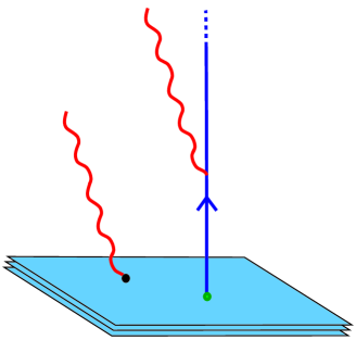
Figure 3: The one-point function in the presence of an external quark is computed with the aid of a string. Each point on the string can be regarded as an individual source. A dilaton detected at infinity may have originated from the string or from the D3-branes, through the one-point function induced by the presence of the external source. See text for discussion.

We focus attention first on the case of a point source, located at some radial position $r^{\prime}$. If desired, it can be regarded as an infinitesimal segment of a string. The one-point function for the entire string will be discussed a little bit later. For concreteness, we consider a source for the dilaton s-wave. Proceeding as in the case of the two-point function, we write down the one-point function with the help of

$$G\left(r,r^{\prime}\right)=G_{0}\left(r,r^{\prime}\right)+G_{0}\left(r,0\right)\Delta_{1,\,r^{\prime}}\left(q^{2}\right),$$ (48)

where $G\left(r,r^{\prime}\right)$ (with $r\rightarrow\infty$) is the supergravity propagation from the source out to infinity, divided into a direct piece through flat space and a piece due to the induced one-point function on the brane, $\Delta_{1,\,r^{\prime}}=\left\langle{\mathcal{O}}_{\phi}\right\rangle$, with ${\mathcal{O}}_{\phi}$ the operator given in (10). The situation is summarized in Fig. 3 (which depicts the entire string). The one-point function is thus computed using

$$\Delta_{1,\,r^{\prime}}\left(q^{2}\right)=\lim_{r\rightarrow\infty}\frac{G\left(r,r^{\prime}\right)-G_{0}\left(r,r^{\prime}\right)}{G_{0}\left(r,0\right)}~{}.$$ (49)

The subscript $r^{\prime}$ on the one-point function indicates the dependence on the radial position of the source. Using the same notation and definitions as in Section 3, the result can be written as

$$\Delta_{1,\,r^{\prime}}\left(q^{2}\right)=\frac{4}{q^{2}r^{\prime 2}}\left(e^{i\left(\theta-\theta_{0}\right)}\frac{1}{A}H^{(1)}\left(\nu,-\ln r^{\prime}/R\right)-\left(H_{2}^{(1)}\left(qr^{\prime}\right)+H_{2}^{(2)}\left(qr^{\prime}\right)\right)\right).$$ (50)

Let us now investigate this one-point function in the limit of large scales, i.e., the IR regime in the holographic dual. To do this we consider expression (50) in the limit of small momentum, $q\ll 1/R$, which implies large distances $x$ after Fourier transforming. We begin by considering $qr^{\prime}\ll 1$ but finite $qR^{2}/r^{\prime}$. This includes the case with a source deep inside the AdS region (i.e. $r^{\prime}\ll R$), and we therefore expect to recover the AdS result. We find that the one-point function takes the form

$$\Delta_{1,\,r^{\prime}}\left(q^{2}\right)=\frac{i\pi}{4q^{2}r^{\prime 2}}H_{2}^{(1)}\left(qR^{2}/r^{\prime}\right)-1,$$ (51)

where we have used the fact that $A=-\frac{16i}{\pi R^{4}q^{4}}$ for small $q$. For the purpose of studying the UV/IR correspondence it is useful to write down the one-point function for spacelike momenta $q^{2}=-p^{2}$, where it becomes

$$\Delta_{1,\,r^{\prime}}\left(-p^{2}\right)=\frac{p^{2}R^{4}}{2r^{\prime 2}}K_{2}\left(pR^{2}/r^{\prime}\right)-1.$$ (52)

The Fourier transform,

$$\frac{1}{\left(2\pi\right)^{3}}\int d^{3}pe^{-i\vec{p}\cdot\vec{x}}\Delta_{1,\,r^{\prime}}\left(-p^{2}\right)=\frac{15R^{8}}{8\pi}\frac{r^{\prime-4}}{\left(x^{2}+R^{4}/r^{\prime 2}\right)^{7/2}},$$ (53)

clearly shows how the radial position of a point source is reflected in the holographic dual: the one-point function describes a blob whose width is of order $R^{2}/r^{\prime}$. This is in accordance with the UV/IR correspondence.

The derivation above used $p\ll 1/R$ and $pr^{\prime}\ll 1$, and it is clear that there will be small distance modifications when $x<R$. However, expression (53) will be valid as long as $x\gg r^{\prime}$ even if $r^{\prime}$ is not small, i.e., even if it is outside of the AdS region. On the other hand, if $r^{\prime}\sim x$ we conclude that the one-point function may be corrected even at large distances. To find out how, we need to consider the one-point function for $p\ll 1/R$, finite $pr^{\prime}$ and hence $pR^{2}/r^{\prime}\ll 1$. This gives

$$\Delta_{1,\,r^{\prime}}\left(-p^{2}\right)=\frac{16R^{4}p^{2}}{3r^{\prime 2}}K_{2}\left(pr^{\prime}\right),$$ (54)

where we have made use of the fact that $\frac{B}{A}-1\sim\frac{2\pi iR^{4}p^{4}}{3}$ for small $p$. After Fourier transforming in $p$ we get

$$\frac{1}{\left(2\pi\right)^{3}}\int d^{3}pe^{-i\vec{p}\cdot\vec{x}}\Delta_{1,\,r^{\prime}}\left(-p^{2}\right)=\frac{20R^{4}}{\pi}\frac{1}{\left(x^{2}+r^{\prime 2}\right)^{7/2}}$$ (55)

for large $r^{\prime}$. Interestingly, the UV/IR correspondence is now reversed, with the size of the blob increasing with the radial position. To summarize: as a source is moved to ever larger values of $r^{\prime}$, the blob first decreases in size, in accord with the usual UV/IR correspondence. But as the source leaves the AdS region, the blob reaches a minimal size of order $R$ and then starts to grow again. According to the standard UV/IR correspondence, the region deep inside of AdS corresponds to the IR of the holographic dual, while the region close to the boundary of AdS corresponds to the UV. With AdS as part of a full three-brane background we can proceed even further out, and according to the above reasoning we will again encounter a region of space that will influence the IR behaviour of the holographic dual. In the concluding section of the paper we will have more to say on the nonstandard UV/IR properties of D3-brane holography, and possible connections with non-commutative geometry.

In view of the modified UV/IR correspondence that we have observed in the D3-brane background, it is also important to consider the result of integrating over the source position, $r^{\prime}$, along the entire string. As discussed above, this corresponds to determining the expectation value of the operator dual to the dilaton s-wave, Eq. (10), in the presence of an external quark. In the AdS limit we find that

$$\left\langle\frac{1}{4}F^{2}\right\rangle = \frac{1}{\sqrt{2}\kappa}\left\langle{\mathcal{O}}_{\phi}\right\rangle=\frac{1}{4\pi\alpha^{\prime}}\int dt^{\prime}dr^{\prime}\Delta_{1,\,r^{\prime}}\left(x\right)$$

$$= \frac{1}{4\pi\alpha^{\prime}}\int dt^{\prime}dr^{\prime}\int\frac{d^{4}k}{\left(2\pi\right)^{4}}\,e^{-ik_{0}t^{\prime}-i\vec{k}\cdot\vec{x}}\Delta_{1,\,r^{\prime}}\left(k_{0}^{2}-\vec{k}^{2}\right)$$

$$= \frac{1}{4\pi\alpha^{\prime}}\int_{0}^{\infty}dr^{\prime}\int\frac{d^{3}k}{\left(2\pi\right)^{3}}e^{-i\vec{k}\cdot\vec{x}}\Delta_{1,\,r^{\prime}}\left(-\vec{k}^{2}\right)=\frac{R^{2}}{16\pi^{2}\alpha^{\prime}x^{4}}=\frac{\sqrt{2g_{YM}^{2}N}}{16\pi^{2}x^{4}}~{},$$

where we have used that the time integral enforces $k_{0}=0$. Note the $\frac{1}{\sqrt{2}\kappa}$ in the first equality which cancels a similar factor in the charge density of the string. These factors come about since we are using a canonically normalized dilaton. The result of the calculation is indeed in agreement with [45], apart from the factor of two mentioned in Section 4.

What happens if we take into account the portion of the string that lies outside of the AdS region? Through the reversed UV/IR correspondence, this threatens to change the large scale behaviour of the one-point function. However, for a given scale $x\gg R$, one can easily estimate the modifications of $\left\langle{\mathcal{O}}_{\phi}\right\rangle$ due to portions of the string with $r^{\prime}>x$, by comparing the integral of (53) and (55) from $r^{\prime}=x$ to $r^{\prime}=\infty$. This shows that any modification will be at most of order $1/x^{6}$, and the coefficient of the leading $1/x^{4}$ term will therefore not be modified.

It would also be interesting to consider the high energy or small distance behaviour of the one-point function. For this we would need to investigate the one-point function (50) in the limit where $q^{2}=-p^{2}$ becomes large and negative. This we have not done; in Section 4 we have already discussed some difficulties in extracting this limit.

6 Higher Correlation Functions

The prescription for two-point functions derived in Section 3 extracts information from the brane geometry by probing it with a bulk correlation function evaluated at points at asymptotic distances from the brane. No relation was assumed between the radial positions of these points. For $n$-point functions we may formulate our prescription in the same way, but it is convenient and perhaps more natural to compute correlators between points on a common cutoff surface. Then we can formulate rules for computing brane $n$-point functions motivated by the same reasoning as before (see Fig. 4):

• Introduce a cutoff surface at $r=r_{\Lambda}$.

• Draw all curved space Feynman diagrams for the $n$-point correlation function of the appropriate supergravity fields. Work in position space for $r$ and in momentum space for $x^{\mu}$. The $n$ external legs have one end at $r=r_{\Lambda}$, and carry four-dimensional momenta $k_{1},\ldots,k_{n}$.

• Replace the propagators $G(k_{i};r_{\Lambda},r)$ associated with external legs by $G_{\Delta}(k_{i};r_{\Lambda},r)$, where $G_{\Delta}=G-G_{0}$, with $G_{0}$ the corresponding flat space propagator.

• Amputate each external leg, dividing by $G_{0}(k_{i};r_{\Lambda},0)$.

• Take the limit $r_{\Lambda}\to\infty$.

Combining rules 3) and 4), the factor on each external leg becomes

$$\Delta_{1,\,r}(k^{2}) = \lim_{r_{\Lambda}\rightarrow\infty}{G_{\Delta}(k;r_{\Lambda},r)\over G_{0}(k;r_{\Lambda},0)}$$

$$= {e^{i(\theta-\theta_{0})}\phi_{1}(r)-2A\phi_{01}(r)\over 2A\phi_{01}(0)}$$

$$= {e^{i(\theta-\theta_{0})}\phi_{3}(r)-\phi_{03}(r)+\frac{B}{A}e^{i(\theta-\theta_{0})}\phi_{2}(r)-\phi_{02}(r)\over\phi_{01}(0)}~{}.$$

The notation here is the same as in Section 3. This factor effectively removes processes where the external leg is unaffected by the presence of the brane. We thus restrict attention to processes where all external lines touch the brane, and from these we extract the physics on the brane.

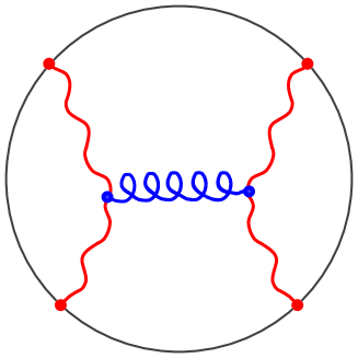
Figure 4: The prescription for $n$-point correlators: Introduce a cutoff surface at asymptotic radial coordinate $r=r_{\Lambda}$. In each of the Feynman diagrams for the $n$-point correlation function of the appropriate supergravity fields, replace all curved space propagators $G$ associated to external legs by $G_{\Delta}=G-G_{0}$. Amputate each external leg, dividing by $G_{0}$. See text for a more precise description.

As an example we write down the case of the three-point function

$$\Delta_{3}(k_{1},k_{2},k_{3})=\lim_{r_{\Lambda}\to\infty}\frac{\int\sqrt{-g}drG_{\Delta}(k_{1};r_{\Lambda},r)G_{\Delta}(k_{2};r_{\Lambda},r)G_{\Delta}(k_{3};r_{\Lambda},r)V_{3}}{G_{0}(k_{1};r_{\Lambda},0)G_{0}(k_{2};r_{\Lambda},0)G_{0}(k_{3};r_{\Lambda},0)}~{},$$ (58)

obtained from the corresponding supergravity three-point function

$$G_{3}(k_{1},k_{2},k_{3};r_{1},r_{2},r_{3})=\int\sqrt{-g}drG(k_{1};r_{1},r)G(k_{2};r_{2},r)G(k_{3};r_{3},r)V_{3}~{},$$ (59)

where $V_{3}$ is the supergravity three-vertex, which generally may involve the metric, momenta in the brane directions and derivatives in the transverse dimensions.

We now want to check that these $n$-point functions agree with known results in the conformal limit, which amounts to showing that the integrals reduce to AdS integrals in the low energy limit $qR\to 0$. To do this more information on the solutions $\phi_{i}$ and $\phi_{i0}$ is needed. We give the arguments for the three-point function, but one can repeat the same steps for any tree diagram, at least for any diagram with interaction vertices directly connected to external legs. For six-point functions and higher there are other diagrams, and the argument is not complete in its present form.

We may use the asymptotics of the Mathieu functions obtainable through the series expansion (100) described in Appendix A, in the limit of small $qr$. To facilitate comparison with the AdS literature we use Euclidean $q^{2}=-p^{2}$ and find

$$\Delta_{1,\,r}(-p^{2})\rightarrow\frac{p^{2}R^{4}}{2r^{\prime 2}}K_{2}\left(pR^{2}/r^{\prime}\right)-1\rightarrow-\left({pR^{2}\over 2r}\right)^{2}.$$ (60)

We note that $\Delta_{1,\,r}(k^{2})$ vanishes for $r\gg pR^{2}$ (if $pr\ll 1$ ). As demonstrated below the contribution from the outer region, $pr\geq 1$, is suppressed for low energies. Thus the effective upper limit of integration for the three-point function in Eq. (58) goes to zero in the low energy limit, and we may use the near horizon limit of the integration measure to find

$$\Delta_{3}^{CFT}(k_{1},k_{2},k_{3})\sim\kappa R^{2}\int drr^{3}V_{3}\Delta_{1,\,r}(q_{1}^{2})\Delta_{1,\,r}(q_{2}^{2})\Delta_{1,\,r}(q_{3}^{2})$$

$$= \kappa\frac{R^{8}}{8}\int dzz^{-5}\left(p_{1}^{2}z^{2}K_{2}(p_{1}z)-2\right)\left(p_{2}^{2}z^{2}K_{2}(p_{2}z)-2\right)\left(p_{3}^{2}z^{2}K_{2}(p_{3}z)-2\right)~{},$$

which scales as $q^{4}$ in the low energy limit. We recognize the AdS form of the three-point function with the bulk-to-boundary propagator $p^{2}z^{2}K_{2}(pz)$. The subtractions found automatically in our approach may look unfamiliar, because they are not always explicitly mentioned. They are however necessary to obtain the final finite conformally invariant results given for instance in [47, 4]. They are all independent of at least one momentum (or at least one relative distance, in position space). Just as in the case of the two-point function, our approach automatically produces a finite answer, in contrast to the standard AdS calculations that require renormalization. Since the region of integration that contributes is entirely within the AdS region, any supergravity vertex $V_{3}$ that yields a conformally invariant three-point function in the AdS case, will do so in our low energy limit, no matter how complicated it is. The three dilaton vertex,the dilaton-${\rm Tr}F^{2}$ coupling, our normalization of $F$ and $\kappa/R^{4}\sim 1/N$ then give

$$\left\langle{\rm Tr}F^{2}{\rm Tr}F^{2}{\rm Tr}F^{2}\right\rangle\sim\frac{1}{N}~{},$$ (62)

as expected.

To see why the region $r\leq pR^{2}$ dominates low energy behaviour we need a qualitative understanding of the wave solutions $\phi_{i}(r)$. This may be obtained directly from their equation of motion [11], written in terms of $\rho=\ln\frac{r}{R}$,

$$\left\{\partial_{\rho}^{2}+2(qR)^{2}\cosh{2\rho}-4\right\}e^{2\rho}\phi_{i}(Re^{\rho})=0~{},$$ (63)

which can be thought of as a one dimensional Schroedinger equation with a potential barrier. For small $qR$ there is oscillatory behaviour for $2r<qR$ and for $qr>2$. The waves tunnel through the barrier between the turning points with an approximate amplitude $\phi(r)=C+DR^{4}/r^{4}$ inside the barrier. For the solution $\phi_{1}$, which is purely ingoing for small $r$, almost all the incident wave is reflected and the amplitude does not grow from the exterior region towards the interior region. This means that $C\gg D$. For the exterior region we use Eqs. (100), (6) and (19), which give

$$I_{ext}\sim\int_{1/q}r^{5}drq_{1}^{4}\Delta_{2}{(q_{1}^{2})}q_{2}^{4}\Delta_{2}{(q_{2}^{2})}q_{3}^{4}\Delta_{2}{(q_{3}^{2})}\frac{H^{(1)}_{2}(q_{1}r)}{(q_{1}r)^{2}}\frac{H^{(1)}_{2}(q_{2}r)}{(q_{2}r)^{2}}\frac{H^{(1)}_{2}(q_{3}r)}{(q_{3}r)^{2}}\sim q^{6}~{},$$ (64)

using $\Delta_{2}(q^{2})={\mathcal{O}}(q^{0})$. The contribution from the barrier region is obtained by matching to the exterior solution at the exterior turning point:

$$I_{bar}\sim\int_{R}^{1/q}r^{5}dr{q_{1}}^{4}{q_{2}}^{4}{q_{3}}^{4}\sim q^{6}~{},$$ (65)

using also Eq. (97). We find as promised that the conformal result (6) from the interior region dominates at low energies.

7 The Quark-Antiquark Potential

In the standard AdS₅/CFT₄ correspondence, an external quark in SYM is dual to a string in the bulk of AdS space. This identification leads to a natural recipe [48, 49] for computing Wilson loops in the strongly-coupled gauge theory, which has been exploited to obtain numerous interesting results (see [51, 4] for a review of some of them). In the present section we wish to generalize the Wilson loop prescription of [48, 49] to our setting, and use it to determine the quark-antiquark potential in the holographic theory.

The motivation for relating strings in the bulk theory to external sources in the four-dimensional theory is of course the same as in the AdS case. Start with $N+1$ coincident D3-branes, and pull one brane out to a finite separation $r_{\Lambda}$, by giving a vacuum expectation value to the appropriate worldvolume scalar field. This breaks $U(N+1)\to U(N)\times U(1)$. A string connecting the solitary brane to the stack of $N$ branes represents a W-boson of the spontaneously broken gauge theory [52]. In the supergravity picture, the $N$ D3-branes are replaced by the black three-brane solution, so the W-boson corresponds to a string extending from the solitary D3-brane at $r=r_{\Lambda}$ down to the horizon at $r=0$. In Section 5 we have already made use of this representation to determine the field around a point source in the dual theory.

We describe the dynamics of a fundamental string through the Nambu-Goto action

$$S_{F}=-T_{F}\int d^{2}\sigma\sqrt{-g^{(i)}}~{},$$ (66)

where $g^{(i)}$ is the pullback of the spacetime metric (3) to the string worldsheet, and $T_{F}={1/2\pi l_{s}^{2}}$ is of course the string tension. We make a static gauge choice $\sigma^{1}=r,\sigma^{2}=t$, and restrict attention to static configurations of the form $X(r)$ (where $x$ is one of the spatial directions parallel to the D3-branes), with the string pointing along a fixed ${\mathbf{S}}^{5}$ direction. In most of the discussion it will be convenient to use an inverted radial coordinate $z=R^{2}/r$. The generic static solution,

$$X(z;z_{m})=\pm\int_{z}^{z_{m}}dz\,\frac{z^{4}+R^{4}}{z^{2}\sqrt{z_{m}^{4}-z^{4}}},$$ (67)

describes a string lying along a geodesic which starts and ends at the location of the probe D3-brane, $r=r_{\Lambda}$ ($z=z_{\Lambda}$), and extends down to a minimum at $r=r_{m}$ (a maximum at $z=z_{m}$), as shown in Fig. 5a. We will eventually take $r_{\Lambda}\to\infty$, to remove the probe brane. The endpoints of the string on this brane are separated by a distance

$$\Delta X(z_{\Lambda};z_{m})=2\int_{z_{\Lambda}}^{z_{m}}dz\,\frac{z^{4}+R^{4}}{z^{2}\sqrt{z_{m}^{4}-z^{4}}}.$$ (68)

For large $r$ the ambient space becomes flat, so the string of course just lies along a straight line, with slope $\Delta x/\Delta r=R^{2}/z_{m}^{2}$. The total energy of the string is

$$U(z_{\Lambda};z_{m})=2T_{F}R^{2}\sqrt{R^{4}+z_{m}^{4}}\int_{z_{\Lambda}}^{z_{m}}\frac{dz}{z^{2}\sqrt{z_{m}^{4}-z^{4}}}~{}.$$ (69)

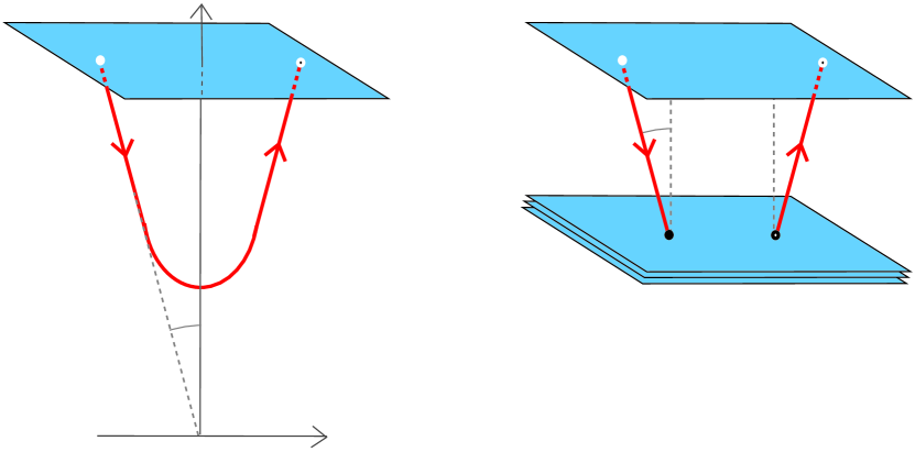
Figure 5: a) ‘Hanging string’ lying along a geodesic of the curved three-brane geometry. The endpoints of the string lie on a probe D3-brane at $r=r_{\Lambda}$. This is the supergravity realization of a W-$\bar{\mbox{W}}$ pair in the $U(N)\times U(1)$ gauge theory. b) The same system in the ‘branes + flat space’ picture: two strings of opposite orientation connect the stack of $N$ D3-branes to a solitary brane a distance $r_{\Lambda}$ away. The endpoints of the strings on the stack of D3-branes constitute a quark-antiquark pair. See text for discussion.

The string we have just described corresponds to a W-$\bar{\mbox{W}}$ pair in the $U(N)\times U(1)$ theory, i.e., a quark-antiquark pair from the perspective of the $U(N)$ theory. As a simple check, notice that if we send $z_{m}\to\infty$ holding $z_{\Lambda}$ fixed, (69) reduces to $2T_{F}R^{2}/z_{\Lambda}=2T_{F}r_{\Lambda}$, which is the correct energy for two infinitely separated W-bosons. In the ‘D-branes $+$ flat space’ picture, the situation is as portrayed in Fig. 5b. The stack of $N$ D3-branes and the solitary brane are separated by a distance $r_{\Lambda}$, with two strings of opposite orientation running between them. The endpoints of these strings which lie on the $N$ D3-branes constitute a quark-antiquark pair in the worldvolume theory, and so attract one another. As a result of this attraction, the strings are tilted by an angle $\alpha=\arctan(R^{2}/z_{m}^{2})$. The endpoints on the probe brane are held in place by an external agent which enforces the appropriate Dirichlet boundary conditions [50]. Because of the tilt, the separation $L$ between the quark and the antiquark is (for large $r_{\Lambda}$) much smaller than that between the endpoints on the solitary brane. As seen in Fig. 5b, the two distances are related by

$$L=\Delta X(z_{\Lambda};z_{m})-2r_{\Lambda}\tan\alpha=\Delta X(z_{\Lambda};z_{m})-{2R^{4}\over z_{\Lambda}z_{m}^{2}}~{}.$$ (70)

We are now ready to compute the quark-antiquark potential. Since we are interested in taking the limit $z_{\Lambda}\to 0$ to remove the probe brane to infinity, we first carry out a Laurent expansion of (68) about $z_{\Lambda}=0$, writing

$$\Delta X(z_{\Lambda};z_{m}) = R^{4}\int_{z_{\Lambda}}^{z_{m}}\frac{2dz}{z^{2}\sqrt{z_{m}^{4}-z^{4}}}+\int_{z_{\Lambda}}^{z_{m}}\frac{2z^{2}dz}{\sqrt{z_{m}^{4}-z^{4}}}.$$

$$= {R^{4}\over z_{m}^{3}}\left\{\int_{0}^{1}{d\zeta\over\zeta^{2}}\left[{2\over\sqrt{1-\zeta^{4}}}-2\right]+2{z_{m}\over z_{\Lambda}}-2\right\}+z_{m}\int_{0}^{1}\frac{2\zeta^{2}d\zeta}{\sqrt{1-\zeta^{4}}}+\ldots,$$

where we omit terms involving positive powers of $z_{\Lambda}$. The two integrals can be carried out analytically, yielding $2-c$ and $c$, respectively, with $c=(2\pi)^{3/2}/[\Gamma(1/4)]^{2}\simeq 1.198$. We are thus left with

$$\Delta X(z_{\Lambda};z_{m})={2R^{4}\over z_{\Lambda}z_{m}^{3}}+c\left(z_{m}-{R^{4}\over z_{m}^{3}}\right)+\ldots$$ (72)

Using this in (70) we obtain a relation between the quark-antiquark separation $L$ and the geodesic parameter $z_{m}$,

$$L(z_{m})=c\left(z_{m}-{R^{4}\over z_{m}^{3}}\right),$$ (73)

which is perfectly well-defined in the limit $z_{\Lambda}\to 0$.

We next Laurent-expand (69),

$$U(z_{\Lambda};z_{m}) = {T_{F}R^{2}\over z_{m}^{3}}\sqrt{R^{4}+z_{m}^{4}}\left\{\int_{0}^{1}{d\zeta\over\zeta^{2}}\left[{2\over\sqrt{1-\zeta^{4}}}-2\right]+2{z_{m}\over z_{\Lambda}}-2\right\}+\ldots$$ (74)

$$= 2T_{F}{R^{2}\over z_{\Lambda}}{\sqrt{R^{4}+z_{m}^{4}}\over z_{m}^{2}}-c{T_{F}R^{2}\over z_{m}^{3}}\sqrt{R^{4}+z_{m}^{4}}+\ldots$$

The leading term diverges in the limit $z_{\Lambda}\to 0$, but it is clearly just the energy $2T_{F}r_{\Lambda}\sec\alpha$ of the two straight strings in Fig. 5b. We are interested only in the energy $E$ which arises from the $U(N)$ interaction between the quark and antiquark, so we subtract this leading term and obtain

$$E(z_{m})=-c{T_{F}R^{2}\over z_{m}^{3}}\sqrt{R^{4}+z_{m}^{4}}~{}.$$ (75)

Eqs. (73) and (75) give the quark-antiquark potential $E(L)$ in implicit form. The potential is plotted in Fig. 6.

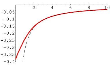
Figure 6: Quark-antiquark potential $E(L)$ in the holographic theory (in $R$=1 units). For large $L$, the potential agrees with that of ${\mathcal{N}}=4$ SYM (dashed line). For short distances there is confining behaviour.

For large $q\bar{q}$ separation, $L\gg R$, both (73) and (75) reduce to the corresponding AdS relations [48, 49], so as required the IR limit of the potential coincides with the conformal ${\mathcal{N}}=4$ potential,

$$E_{IR}(L)=-{c^{2}\over\sqrt{2}\pi}{\sqrt{g_{YM}^{2}N}\over L}~{}.$$ (76)

Here we have made use of the relation $R^{4}=2g_{YM}^{2}Nl_{s}^{4}$ to write the result exclusively in terms of gauge theory quantities.

At the opposite extreme, notice from (73) that, surprisingly, $L\to 0$ as $z_{m}\to R$. Geodesics with $z_{m}<R$ thus appear to give no direct information about the quark-antiquark interaction in the $U(N)$ theory. Since these geodesics are completely outside the throat region $z\geq R$, this is yet another indication that the flat space region is in a sense left out of the holographic theory. This is as expected from the decoupling argument of Section 2, and is indeed consistent with what we have found for correlation functions in Sections 3 through 6. The short-distance quark-antiquark potential is

$$E_{UV}(L)=-{c\sqrt{g_{YM}^{2}N}\over\pi R}+{\sqrt{g_{YM}^{2}N}\over 2\pi R^{2}}L~{}.$$ (77)

This expression is again written only in terms of parameters of the gauge theory, and displays confining behaviour with a confining string tension $\sigma=\sqrt{g_{YM}^{2}N}/2\pi R^{2}$. From the supergravity perspective this result is not surprising, as $\sigma=T_{F}/\sqrt{2}$ is simply the tension of a fundamental string located at $r=R$.

From (73) and (75) it follows that the quark and antiquark attract one another with a force

$$\frac{\partial E}{\partial L}=\frac{T_{F}R^{2}}{\sqrt{R^{4}+z_{m}^{4}}}~{}.$$ (78)

As a consistency check on our approach, we note that this equals the force $\partial U/\partial\Delta X$ obtained from the unsubtracted expressions (68) and (69) in the $z_{\Lambda}\to 0$ limit.

8 The Baryon

In the preceding section we have seen how the AdS picture of a quark-antiquark pair can be generalized away from the conformal limit. We now wish to point out that it is also possible to extend the AdS description of the baryon [53, 54, 55, 56] to our setting.

In the AdS₅/SYM₄ correspondence, the $SU(N)$ baryon (the color-neutral coupling of $N$ external quarks) is dual to $N$ fundamental strings stretching from the AdS boundary to a D5-brane wrapped around ${\mathbf{S}}^{5}$ [53, 54]. To provide a thorough description of this system it is necessary to analyse the full worldvolume action for the D5-brane embedded in AdS${}_{5}\times{\mathbf{S}}^{5}$. The baryon is then seen to be realized as a particular class of BPS D5-brane embeddings [55, 56, 57, 58], in which the $N$ strings appear as Born-Infeld string tubes [59, 60].

In our case, then, to obtain a picture of the baryon we must consider a D5-brane embedded in the full three-brane background. It was shown in [56, 57, 61] that this system has a one-parameter family of BPS solutions of the form $\zeta=\zeta(\xi;\zeta_{\Lambda})$, where $\zeta=-r\cos\theta$, $\xi=r\sin\theta$, with $\theta$ the polar angle on ${\mathbf{S}}^{5}$. These embeddings have a flat portion and (for $\zeta_{\Lambda}>0$) a tubular region, which as explained in [56] represent a flat D5-brane located at $\zeta=\zeta_{\Lambda}$, and a bundle of $N$ Born-Infeld strings, respectively (see Fig. 7).

Figure 7: Family of D5-branes embedded in the full D3-brane geometry. The solutions extend along $r$ and the ${\mathbf{S}}^{5}$ directions, and lie at a fixed position along $\bf x$. They are parametrized as $\zeta=\zeta(\xi;\zeta_{\Lambda})$, where $\zeta=-r\cos\theta$, $\xi=r\sin\theta$, with $\theta$ the polar angle on ${\mathbf{S}}^{5}$. $\zeta_{\Lambda}$ denotes the vertical position of the flat region of the D5-brane. The tubular portion of the brane, in the limit $\zeta_{\Lambda}\to\infty$, is dual to the baryon of the holographic theory.

We propose that these solutions are dual to the baryon of the holographic theory, with the understanding that the flat D5-brane at $\zeta=\zeta_{\Lambda}$ plays the same role as the solitary D3-brane at $r=r_{\Lambda}$ in the quark-antiquark case, and should therefore be removed by taking $\zeta_{\Lambda}\to\infty$. For large $\zeta_{\Lambda}$, the lower portion of the tube is close to $r=0$, and coincides with the AdS baryon embedding. This is a necessary condition for the large-distance field of the baryon to reduce to that of the SYM theory. In the limit $\zeta_{\Lambda}\to\infty$, the Born-Infeld tube becomes infinitely thin.

It was demonstrated in [56, 57] that the energy of the tube (obtained from the full energy by subtracting the infinite contribution of the flat portion) is exactly equal to the energy of $N$ fundamental strings of length $\zeta_{\Lambda}$. Since these strings represent the baryon’s constituent quarks, it follows that the D3 baryon (just like its AdS counterpart) has zero binding energy, as expected from the BPS character of the configuration.

9 Discussion

Based on the assumption that there exists some theory which holographs the full asymptotically flat three-brane background, in this paper we have developed methods for computing quantities in the dual theory in terms of supergravity. Concretely, in Section 6 we have presented a calculational recipe for arbitrary $n$-point correlators in the holographic dual. The particular case of two-point functions of the operators ${\mathcal{O}}_{\phi}$ coupling to dilaton partial waves was analysed at length in Sections 3 and 4. Three-point functions were discussed in Section 6, and a one-point function in the presence of a source was examined in Section 5. Additionally, in Section 7 we have employed a ‘hanging’ string to determine the potential energy of an external quark-antiquark pair in the dual theory, and in Section 8 we have commented on the representation of baryons as deformed D5-branes.

In addition to its derivation, we have presented several non-trivial checks of our recipe for correlation functions. First, the correlators we obtain reduce to ${\mathcal{N}}=4$ SYM correlators in the extreme low-energy limit. Second, the two-point functions of operators dual to dilaton partial waves are related to the corresponding exact absorption probabilities [11] through the appropriate optical theorem. Third, our prescription incorporates a natural subtraction and amputation procedure which automatically removes potential UV divergences and renders the correlators well-defined.

Despite these nice features, our results are not entirely satisfactory. The correlators we obtain appear to include terms which are analytic functions of the momenta with imaginary coefficients. As explained in Section 4, their presence is related to the so-called Stokes phenomenon [42], which in some cases forces subleading coefficients of the asymptotic expansion of a real function to take on complex values. We should emphasize that the appearance of such terms is not unique to our approach: the two-point functions derived in [37, 38] using the GKPW recipe [2, 3] suffer from the same problem (a fact which was not noticed in those works). Given that the problematic terms are analytic in momentum-space, and therefore amount to contact terms, one is tempted to simply drop them from the correlators. This would indeed yield $n$-point functions with sensible analytic structure. The only problem is that these same contact terms appear to be necessary for two-point functions to be correctly related to the corresponding absorption probabilities, as dictated by the optical theorem. We have discussed this puzzle in Section 4, as well as some of its possible resolutions.

Our work was motivated by a series of recent papers [10, 16, 11, 12] addressing the possible generalization of the AdS₅/SYM₄ correspondence away from the conformal limit $\omega R\to 0$. As explained in Section 2, the authors of [10, 16, 11] espouse the view that physics on the full three-brane background is encoded in the D3-brane worldvolume action (an insight which was implicit already in [7]). Through considerations of symmetries and large anomalous dimensions, Gubser and Hashimoto [11] were led to conjecture that, for strong ’t Hooft coupling, this worldvolume theory is simply ${\mathcal{N}}=4$ SYM deformed in the infrared by a specific dimension-eight operator, as indicated in (7). They advocate a duality between this theory and supergravity in the full three-brane background, which is supposed to hold in the limit $g_{s}\to 0$, $g_{s}N\to\infty$.

We wish to stress that our work does not rely on the specific form of the conjecture of [11]. Since our calculations are based on the supergravity side of the duality relation, the physical quantities we compute pertain to whatever theory turns out to be dual to the curved space description, even if it is not precisely of the form (7). We regard our work as a step towards the more precise specification of this theory, and it is an outstanding challenge to reproduce our results through an explicit field theory calculation.

On the other hand, it should be noted that our approach is in accord with the perspective of [10, 16, 11] in two important respects: first, throughout the paper we explicitly assume that the worldvolume theory of D3-branes (or at least some localized $(3+1)$-dimensional object) is relevant for the duality; second, for the most part we restrict attention to the limit $g_{s}\to 0$. These two assumptions play a role both in our derivation of the recipe for two-point functions in Section 3, and in our formulation of the optical theorem in Section 4.

The duality we have studied in this paper operates between two alternative descriptions of physics in the presence of a system of $N\gg 1$ branes: on the one hand, supergravity on the curved three-brane background; on the other hand, the D3-brane worldvolume theory coupled to supergravity in the bulk of flat $(9+1)$-dimensional space. We are interested in this system at finite $\omega R$, since $\omega R\to 0$ is just the usual Maldacena limit [1]. An important aspect that follows from our analysis (see Section 3) is that, for large $g_{s}N$, the worldvolume theory does not decouple from the bulk even if $g_{s}\to 0$. As a result, $n$-point correlators of operators in the lower-dimensional theory receive contributions from virtual particles propagating in the higher-dimensional space, which cannot be disentangled from those entirely confined to the brane. As explained in Section 4, such higher-dimensional processes also have an impact on the form of the optical theorem connecting two-point functions to absorption probabilities, a fact which was overlooked in [11].

The lack of a complete decoupling should not be mistaken for the absence of a duality. It does however indicate that, in contrast with the AdS/CFT case, the ‘gauge theory’ side of the duality in question necessarily involves both the worldvolume theory and supergravity in flat space. Of course, as $g_{s}\to 0$ the latter theory becomes trivial— free fields propagating in $(9+1)$-dimensional flat space. Roughly speaking, this trivial part of the system describes the free fields on the asymptotically flat part of the three-brane geometry, while the worldvolume theory encodes all the non-trivial physics in the throat (which includes much more than the near-horizon geometry relevant to the standard AdS/CFT correspondence [1]). If correct, this is undoubtedly a very profound statement. In particular, it still seems appropriate to us to speak of ‘holography’, given that the non-trivial aspects of a higher-dimensional theory are encoded in the dynamics of a theory which is essentially four-dimensional.

Intriligator [12] has argued that the duality conjectured by Gubser and Hashimoto should in fact be expected to hold for arbitrary $g_{s}$ and $N$. In Section 2 we have reviewed his arguments and commented on the problematic aspects of his proposal. Here we wish to emphasize that Intriligator arrived at his conjecture by means of scaling and non-renormalization arguments which do not explicitly bring the two alternative D-brane descriptions into play. While he asserts that the dual theory is of the form (7), he does not identify it with the D3-brane worldvolume theory. This could perhaps be viewed as a weakness of his proposal, but it enables him to take the view that the four-dimensional theory whose Lagrangian is (7), is by itself (without any coupling to a higher-dimensional theory) dual to the entire three-brane background. While we approach the problem from a different perspective, the interesting question remains whether there could exist a purely four-dimensional theory which holographs the full asymptotically flat geometry. From our analysis it is clear that such a theory would necessarily be more than a pure D3-brane worldvolume theory, for it would have to summarize the effective theory on the branes, free supergravity in $(9+1)$-dimensional flat space, and the interaction between them. In such a theory our correlators would be seen to follow from a strictly four-dimensional calculation.

In this connection, we cannot resist commenting on the similarity between certain aspects of our results and some recent analyses of non-commutative field theories. A first point to notice is the potential connection of our work and that of Maldacena and Russo [38], who studied certain supergravity backgrounds which are the putative duals of large $N$ non-commutative gauge theories (this was first done in [62]). The backgrounds in question are obtained as decoupling limits of the solution describing $N$ D3-branes in the presence of a constant $B$ field — the same limit which on the gauge theory side gives rise to the non-commutative description [63]. Among other things, the authors of [38] computed a two-point correlator of a certain component of the gauge theory energy-momentum tensor, employing an extrapolation of the GKPW recipe [2, 3]. Interestingly, the relevant supergravity field (restricted to be independent of time and one spatial direction) satisfies an equation which is identical to that of a dilaton propagating on the full (zero $B$ field) asymptotically flat D3-brane background! As a result, the correlator obtained in [38] is essentially the same as that computed by us in Section 3, and expressed in Eq. (29). Maldacena and Russo also determined the shape and energy of strings lying along geodesics of their geometry; the relevant equations happen to have the same form as those considered by us in our study of the quark-antiquark potential (see Section 7). It is too soon to tell whether these remarkable similarities are merely accidental or indicate some underlying connection. It should be emphasized that the backgrounds studied in [62, 38] are completely different from ours: not only is there a non-vanishing $B$ field (whose magnitude is in fact taken to diverge in the decoupling limit), but also a dilaton with non-trivial dependence on the radial coordinate. Still, it is interesting to note that, as pointed out in [62], the Einstein frame metric in one case is asymptotically flat.

There is yet another feature of our results which is suggestive of a relation to the non-commutative case: the presence, in what is otherwise a four-dimensional theory, of virtual particles propagating in a higher-dimensional space. This closely resembles a phenomenon encountered in recent studies of non-commutative perturbative dynamics [64, 65] (see also [66]–[76]). In that context, the basic observation is that while the non-commutativity removes the usual UV field-theoretic divergences, it gives rise (even in a massive theory) to peculiar IR divergences. The latter represent novel long-distance effects which in fact arise from the short-distance degrees of freedom— an intriguing phenomenon known as UV/IR mixing [64, 65]. To capture the correct long-distance physics in a Wilsonian description of the theory with an explicit UV cutoff, it is then necessary to introduce additional fields which reproduce the unfamiliar IR singularities. Some of these fields have propagators which can be naturally interpreted as describing particle propagation in a higher-dimensional space. This suggests an analogy with string theory, associating the lower-dimensional fields with open strings attached to a brane, and the higher-dimensional fields with closed strings which can propagate outside the brane. There is thus a clear parallel with the ‘branes $+$ flat space’ description of our system, which incorporates worldvolume and bulk degrees of freedom in manifest correspondence with massless modes of open and closed strings, respectively.

The imprint of UV/IR mixing is seen also in the context of our discussion of the UV/IR correspondence in Section 5. As explained there, a point-like source located at radial position $r=r^{\prime}$ in the bulk makes its primary contribution to a one-point function in the dual theory at a length scale $L(r^{\prime})$ which is essentially the maximum of $R^{2}/r^{\prime}$ and $r^{\prime}$. This means in particular that the $r^{\prime}\to\infty$ region, which would be naturally interpreted as a high-energy region in the holographic dual, can in fact give rise to the large-distance effects.

We reiterate that all similarities with the non-commutative case might amount to no more than an intriguing analogy. It is however tempting to speculate that a) perhaps there exists a purely four-dimensional theory which holographs the entire three-brane background (flat region included), and b) possibly this theory incorporates some type of non-commutativity. The dual description that we have directly scrutinized — the one which follows directly from D-brane reasoning — could then be regarded as a reformulation of the non-commutative dual in terms of two coupled components: a Wilsonian worldvolume effective action (which according to [11] is given by (7), with a cutoff of order $1/R$), and the $(9+1)$-dimensional flat space supergravity action, encoding the additional long-distance effects. This interpretation would be in line with the fact that, as explained in Sections 4 and 5, there is a subtlety in extracting low-energy results from the supergravity description. If we regard AdS space as the $r\to 0$ portion of the full three-brane geometry, carry out calculations in the complete background, and then take the low-energy limit, the results do not necessarily agree with those obtained in a space which is purely AdS from the beginning. In the ‘branes $+$ flat space’ side of the duality, the issue is whether or not one includes the contribution of the virtual particles which propagate off the branes. In the hypothetical strictly four-dimensional description, this would correspond to the statement that the non-commutative theory does not reduce to the naive commutative description at low energies.

Before closing, we wish to remark that our prescription for correlation functions is based on such simple considerations that it seems possible to generalize it to arbitrary asymptotically flat backgrounds. Of course, in the general case one is no longer guided by D-brane intuition, so the attempt to describe the curved background in terms of a lower-dimensional effective theory embedded in a higher-dimensional flat space is more of a guess— even if it is still in consonance with the spirit of [34, 35]. But it is the very fact that it would take us into uncharted terrain which could possibly make this investigation worth our while.

10 Acknowledgements

We are grateful to Nadav Drukker, Ansar Fayyazuddin, Hans Hansson, Esko Keski-Vakkuri, Subir Mukhopadhyay, Øyvind Tafjord, and Staffan Yngve for useful discussions. We would also like to thank Karen Ramírez for help with the figures. The work of U.D., A.G., and B.S. was supported by the Swedish Natural Science Research Council (NFR), and that of M.K. by the Swedish Foundation for International Cooperation in Research and Higher Education (STINT).

Appendix A

In this appendix we review some properties of Mathieu functions following [77, 11, 26]. In [11] it was realized that the radial equation for a massless field moving in the D3-brane background,

$$\left[\frac{d^{2}}{dr^{2}}+\frac{5}{r}\frac{d}{dr}-\frac{l(l+4)}{r^{2}}+q^{2}\left(1+\frac{R^{4}}{r^{4}}\right)\right]\phi(r)=0,$$ (79)

can be recast as Mathieu’s equation

$$\left[\frac{d^{2}}{d\rho^{2}}+2(qR)^{2}\cosh(2\rho)-(l+2)^{2}\right]\psi(\rho)=0,$$ (80)

by means of the change of variables

$$r=Re^{\rho},\ \ \ \phi(r)=e^{-2\rho}\psi(\rho).$$ (81)

Following [77] a solution can be easily written as an expansion for small $qR$ :

$$u(\rho) = \sum_{n=0}^{\infty}(qR)^{2n}u_{n}(\rho),$$ (82)

$$u_{0}(\rho) = \cosh((l+2)\rho),$$ (83)

$$u_{n}(\rho) = -\frac{2}{l+2}\int_{0}^{\rho}\cosh(2\rho^{\prime})\sinh((l+2)(\rho-\rho^{\prime}))u_{n-1}(\rho^{\prime})d\rho^{\prime}~{}.$$ (84)

A Floquet solution, namely one satisfying

$$M_{\nu}(\rho+i\pi)=e^{i\pi\nu}M_{\nu}(\rho),$$ (85)

can be obtained from $u(\rho)$ as

$$M_{\nu}(\rho)=u(\rho)-e^{i\pi\nu}u(\rho+i\pi),$$ (86)

where the Floquet exponent $\nu$ turns out to be

$$\nu=\frac{1}{\pi}\arccos(u(i\pi)).$$ (87)

This solution can be expanded as

$$M_{\nu}(\rho)=\sum_{n=-\infty}^{\infty}a_{n}e^{(2n+\nu)\rho}~{},$$ (88)

where the coefficients $a_{n}$ can be easily identified from the expansion in powers of $qR$ given above. A linearly independent solution to (80) is given by

$$M_{-\nu}(\rho)\equiv\sum_{n=-\infty}^{\infty}a_{-n}e^{(2n-\nu)\rho}~{},$$ (89)

where the $a_{n}$ are the same coefficients as in (88).

For ease of comparison, we note that the Floquet solution $J(\nu,\rho)$ given in [11] is proportional to $M_{\nu}$. The former is defined as

$$J(\nu,\rho)=\sum_{n=-\infty}^{\infty}(-)^{n}\varphi(n+{\textstyle{1\over 2}}\nu)e^{(2n+\nu)\rho}~{},$$ (90)

so the two solutions are related through

$$a_{0}J(\nu,\rho)=\varphi(\nu/2)M_{\nu}(\rho)\quad\Longrightarrow\quad(-)^{n}\frac{\varphi(n+\nu/2)}{\varphi(\nu/2)}=\frac{a_{n}}{a_{0}}~{}.$$ (91)

$M_{\nu}$ is similarly related to the Floquet solution $Me_{\nu}$ defined in [26].

An alternative expansion in terms of Bessel functions which uses the same coefficients is [11, 26]

$$M_{\nu}(\rho)=\frac{1}{\varphi(\nu/2)}\sum_{n=-\infty}^{\infty}(-)^{n}{a_{n}}J_{n}(qRe^{-\rho})J_{n+\nu}(qRe^{\rho})~{}.$$ (92)

Evaluating this equation at $\rho=0$ and dividing it by the corresponding equation for $M_{-\nu}(0)=M_{\nu}(0)$, the important quantity $\chi$ follows as

$$\chi\equiv\frac{\varphi(-\nu/2)}{\varphi(\nu/2)}={{\sum_{n=-\infty}^{\infty}(-)^{n}a_{-n}J_{n}(qR)J_{n-\nu}(qR)}\over{\sum_{n=-\infty}^{\infty}(-)^{n}a_{n}J_{n}(qR)J_{n+\nu}(qR)}}~{}.$$ (93)

The above expression contains only integer powers of $qR$ except for the factors $(qR)^{\nu}$ and $(qR)^{-\nu}$ arising from the Bessel functions $J_{n\pm\nu}(qR)$. It is possible then to write $\chi$ as

$$\chi=(qR)^{-2\nu}\tilde{\chi}((qR)^{2})=e^{-2\nu\ln(qR)+i\alpha}$$ (94)

where $\tilde{\chi}$ (or $\alpha$) can be expressed as a series expansion in integer powers of $(qR)^{2}$. For generic $l>0$ one obtains (following [26])

$$\nu = l+2-\frac{(qR)^{4}}{4(l+1)(l+2)(l+3)}+\cdots$$ (95)

$$\chi = (-)^{l+1}\frac{l!(l+1)!}{(l+3)}\frac{2^{2l+2}}{(qR)^{2l}}\left[1+\frac{q^{4}}{4(l+1)(l+2)(l+3)}\ln(qR)^{2}\right]+\cdots$$ (96)

which are useful expressions when computing the AdS limit. In the case of $l=0$ one obtains

$$\nu = 2+i\mu~{},$$ (97)

$$\chi = e^{-2i\mu\ln\left[(qR)^{2}e^{\gamma}\right]}\left[-\frac{2}{3}-\frac{1}{3}i\sqrt{5}+(-\frac{49}{1152}+\frac{49}{2880}i\sqrt{5})(qR)^{4}\right.$$ (98)

$$\left.+(\frac{18853}{39813120}i\sqrt{5}+\frac{12527}{9953280})(qR)^{8}+{\mathcal{O}}((qR)^{12})\right]~{},$$

$$\mu = -\frac{\sqrt{5}}{48}(qR)^{4}+\frac{7}{138240}\sqrt{5}(qR)^{8}+\frac{11851}{637009920}\sqrt{5}(qR)^{12}+{\mathcal{O}}((qR)^{16})~{},$$ (99)

where $\gamma\approx 0.5772$ is Euler’s constant.

In the text we also used the solutions [11]

$$H^{(1,2)}(\nu,\rho)=\sum_{n=-\infty}^{\infty}(-)^{n}{a_{n}\over a_{0}}J_{n}(qRe^{-\rho})H^{(1,2)}_{n+\nu}(qRe^{\rho}),$$ (100)

where $H^{(i)}_{n+\nu}$ are Hankel functions of order $n+\nu$. The Mathieu functions $H^{(1,2)}(\nu,\rho)$ are of particular interest because they behave asymptotically as purely ingoing or outgoing waves.

Appendix B

In this appendix we derive Eq. (30). To this end it is useful to first summarize some formulas involving the spherical harmonics on ${\mathbf{S}}^{5}$, following [78]. In the following we denote coordinates parallel and orthogonal to the brane as $x^{\mu}$ and $\vec{y}$, respectively. Besides we write $\vec{y}=r\hat{y}$, with $\hat{y}$ a unit vector. Orthonormal spherical harmonics on ${\mathbf{S}}^{5}$ are then defined through

$$Y_{l{\mathbf{m}}}=\frac{1}{\sqrt{{\mathcal{N}_{l}}}}C^{i_{1}\ldots i_{l}}_{l{\mathbf{m}}}\hat{y}_{i_{1}}\ldots\hat{y}_{i_{l}}~{},$$ (101)

with

$${\mathcal{N}_{l}} = \frac{\pi^{3}}{2^{l-1}(l+1)(l+2)}~{},$$ (102)

$$\int d^{5}\Omega Y_{l{\mathbf{m}}}Y^{*}_{l^{\prime}{\mathbf{m}}^{\prime}} = \delta_{ll^{\prime}}\delta_{{\mathbf{m}}{\mathbf{m}}^{\prime}}~{},$$ (103)

$$\sum_{i_{1}\ldots i_{l}}C_{l{\mathbf{m}}}^{i_{1}\ldots i_{l}}C_{l{\mathbf{m}}^{\prime}}^{i_{1}\ldots i_{l}} = \delta_{{\mathbf{m}}{\mathbf{m}}^{\prime}}~{}.$$ (104)

The coefficients $C^{i_{1}\ldots i_{l}}_{l{\mathbf{m}}}$ take the symmetric traceless part of the product of the unit vectors $\hat{y}$. For a wave incident along $y_{9}$ it is important to compute $\sum_{{\mathbf{m}}}C^{9\ldots 9}_{l{\mathbf{m}}}C^{9\ldots 9}_{l{\mathbf{m}}}$ This calculation was performed in [41] using other coefficients that can be defined by

$$C^{i_{1}\ldots i_{l}}_{p_{1}\ldots p_{l}}=\sum_{{\mathbf{m}}}C_{l{\mathbf{m}}}^{i_{1}\ldots i_{l}}C_{l{\mathbf{m}}}^{p_{1}\ldots p_{l}}~{}.$$ (105)

Translating to the notation used here, the result in [41] reads

$$\sum_{{\mathbf{m}}}C^{9\ldots 9}_{l{\mathbf{m}}}C^{9\ldots 9}_{l{\mathbf{m}}} = \sum_{i_{1}\ldots i_{l}}\sum_{{\mathbf{m}}}C^{9\ldots 9}_{l{\mathbf{m}}}C_{l{\mathbf{m}}}^{i_{1}\ldots i_{l}}\sum_{{\mathbf{m}}^{\prime}}C^{9\ldots 9}_{l{\mathbf{m}}^{\prime}}C_{l{\mathbf{m}}^{\prime}}^{i_{1}\ldots i_{l}}=\sum_{i_{1}\ldots i_{l}}C^{9\ldots 9}_{i_{1}\ldots i_{l}}C^{9\ldots 9}_{i_{1}\ldots i_{l}}$$ (106)

$$= \frac{(l+2)(l+3)}{3\cdot 2^{l+1}}~{}.$$

Now we proceed to derive Eq. (30). When the interaction is

$$S_{\mathrm{int}}=\int d^{4}x\left.{\sum_{{i_{1\dots l}=5}}^{9}}\partial_{i_{1}\ldots i_{l}}\phi(x,y)\right|_{y=0}C^{i_{1}\ldots i_{l}}_{l{\mathbf{m}}}{\mathcal{O}}^{l{\mathbf{m}}}~{},$$ (107)

the analog of (11) turns out to be

$$G(r,r^{\prime},\hat{y},\hat{y}^{\prime}) = G_{0}(r,\hat{y};r^{\prime},\hat{y}^{\prime})$$

$$+\left.\partial_{i_{1}\ldots i_{l}}G_{0}(r,\hat{y};\vec{y}_{1})\right|_{\vec{y}_{1}=0}\sum_{l{\mathbf{m}}}C^{i_{1}\ldots i_{l}}_{l{\mathbf{m}}}\Delta_{2}^{(l)}C^{j_{1}\ldots j_{l}}_{l{\mathbf{m}}}\left.\partial_{j_{1}\ldots j_{l}}G_{0}(r^{\prime},\hat{y}^{\prime};\vec{y}_{2})\right|_{\vec{y}_{2}=0}~{}.$$

The flat space propagator $G_{0}$ can be expanded as

$$G_{0}(r,\hat{y};r^{\prime},\hat{y}^{\prime})=-i\frac{\pi}{2}\frac{1}{(rr^{\prime})^{2}}\sum_{l{\mathbf{m}}}J_{l+2}(qr_{<})H^{(1)}_{l+2}(qr_{>})Y_{l{\mathbf{m}}}(\hat{y})Y_{l{\mathbf{m}}}(\hat{y}^{\prime})$$ (109)

where $r_{<}$ ($r_{>}$) is the smaller (larger) of $r$ and $r^{\prime}$. The Bessel function $J_{l+2}$ ensures that the propagator is well behaved at $r=0$ and the Hankel function $H^{(1)}_{l+2}$ that the flux at infinity is outgoing. From the previous equation and (101) one can compute

$$\left.\partial_{i_{1}\ldots i_{l}}G_{0}(r,\hat{y};\vec{y})\right|_{\vec{y}=0}=-i\frac{\pi}{2}\frac{l!}{(l+2)!}\frac{q^{l+2}}{2^{l+2}}\frac{1}{r^{2}}H_{l+2}(qr)\frac{1}{\sqrt{{\mathcal{N}_{l}}}}C^{i_{1}\ldots i_{l}}_{l{\mathbf{m}}}Y_{l{\mathbf{m}}}(\hat{y}).$$ (110)

Expanding the full propagator in spherical harmonics,

$$G(r,\hat{y};r^{\prime},\hat{y}^{\prime})=\sum_{l{\mathbf{m}}}G^{(l)}(r,r^{\prime})Y_{l{\mathbf{m}}}(\hat{y})Y_{l{\mathbf{m}}}(\hat{y}^{\prime})~{},$$ (111)

it follows that the coefficients $G^{(l)}(r,r^{\prime})$ satisfy

$$\left[\frac{d^{2}}{dr^{2}}+\frac{5}{r}\frac{d}{dr}-\frac{l(l+4)}{r^{2}}+q^{2}\left(1+\frac{R^{4}}{r^{4}}\right)\right]G^{(l)}(r,r^{\prime})=\frac{\delta(r-r^{\prime})}{\pi^{3}r^{5}},$$ (112)

As in Section 3, $G^{(l)}(r,r^{\prime})$ must reduce to a purely ingoing wave at the horizon and a purely outgoing wave at infinity. Again using the notation of Eq. (18), the solution is

$$G^{(l)}(r,r^{\prime})={1\over w_{32}}\phi_{2}(r_{>})\left[\phi_{3}(r_{<})+{B\over A}\phi_{2}(r_{<})\right],$$ (113)

Expanding for large $r$,$r^{\prime}$ and using the values of $A$ and $B$ from (22) the difference between the full and flat space propagators follows as ($r,r^{\prime}\rightarrow\infty$):

$$G^{(l)}(r,r^{\prime})-G_{0}^{(l)}(r,r^{\prime})\simeq\frac{i\pi}{4}\frac{2}{\pi q}\frac{1}{(rr^{\prime})^{\frac{5}{2}}}(-)^{l}e^{iq(r+r^{\prime})}\left[(-)^{l}\frac{\chi_{l}-\frac{1}{\chi_{l}}}{\eta_{l}\chi_{l}-\frac{1}{\eta_{l}\chi_{l}}}-1\right]~{}.$$ (114)

Finally, inserting the last equation and (110) into the expansion (Appendix B), the propagator $\Delta_{2}^{(l)}$ is found to be

$$\Delta_{2}^{(l)}=2^{l+5}\pi^{2}(l+1)(l+2)q^{-2l-4}i\left[(-)^{l}\frac{\chi_{l}-\frac{1}{\chi_{l}}}{\eta_{l}\chi_{l}-\frac{1}{\eta_{l}\chi_{l}}}-1\right]~{}.$$ (115)

References

- [1] J. Maldacena, “The Large Limit of Superconformal Field Theories and Supergravity,” Adv. Theor. Math. Phys. 2 (1998) 231, hep-th/9711200.
- [2] S. S. Gubser, I. R. Klebanov, and A. M. Polyakov, “Gauge Theory Correlators from Noncritical String Theory,” Phys. Lett. B428 (1998) 105, hep-th/9802109.
- [3] E. Witten, “Anti-de Sitter Space and Holography,” Adv. Theor. Math. Phys. 2 (1998) 253, hep-th/9802150.
- [4] O. Aharony, S. S. Gubser, J. Maldacena, H. Ooguri and Y. Oz, “Large N field theories, string theory and gravity,” hep-th/9905111.
- [5] J. Polchinski, “Dirichlet-Branes and Ramond-Ramond Charges,” Phys. Rev. Lett. 75, 4724 (1995), hep-th/9510017.
- [6] S. S. Gubser, I. R. Klebanov and A. W. Peet, “Entropy and Temperature of Black 3-Branes,” Phys. Rev. D54, 3915 (1996), hep-th/9602135.
- [7] I. R. Klebanov, “World-volume approach to absorption by non-dilatonic branes,” Nucl. Phys. B496, 231 (1997), hep-th/9702076.
- [8] S. S. Gubser, I. R. Klebanov and A. A. Tseytlin, “String theory and classical absorption by three-branes,” Nucl. Phys. B499, 217 (1997), hep-th/9703040.
- [9] S. S. Gubser and I. R. Klebanov, “Absorption by branes and Schwinger terms in the world volume theory,” Phys. Lett. B413, 41 (1997), hep-th/9708005.
- [10] S. S. Gubser, A. Hashimoto, I. R. Klebanov and M. Krasnitz, “Scalar absorption and the breaking of the world volume conformal invariance,” Nucl. Phys. B526, 393 (1998), hep-th/9803023.
- [11] S. S. Gubser and A. Hashimoto, “Exact absorption probabilities for the D3-brane,” Commun. Math. Phys. 203 (1999) 325, hep-th/9805140.
- [12] K. Intriligator, “Maximally supersymmetric RG flows and AdS duality,” hep-th/9909082.
- [13] W. I. Taylor and M. Van Raamsdonk, “Multiple Dp-branes in weak background fields,” hep-th/9910052.
- [14] R. C. Myers, “Dielectric-branes,” JHEP 9912, 022 (1999), hep-th/9910053.
- [15] A. Hashimoto and I. R. Klebanov, “Scattering of strings from D-branes,” Nucl. Phys. Proc. Suppl. 55B, 118 (1997), hep-th/9611214.
- [16] S. P. de Alwis, “Supergravity, the DBI action and black hole physics,” Phys. Lett. B435, 31 (1998), hep-th/9804019.
- [17] L. Susskind and E. Witten, “The Holographic Bound in Anti-de Sitter Space,” hep-th/9805114.
- [18] A. W. Peet and J. Polchinski, “UV/IR relations in AdS dynamics,” Phys. Rev. D59, 065011 (1999), hep-th/9809022.
- [19] A. Hashimoto, “Holographic description of D3-branes in flat space,” Phys. Rev. D60, 127902 (1999), hep-th/9903227.
- [20] M. S. Costa, “Absorption by double-centered D3-branes and the Coulomb branch of SYM theory,” hep-th/9912073.
- [21] M. S. Costa, “A Test of the AdS/CFT Duality on the Coulomb Branch,” hep-th/0003289.
- [22] A. A. Tseytlin, “Born-Infeld action, supersymmetry and string theory,” hep-th/9908105.
- [23] H. J. Kim, L. J. Romans and P. van Nieuwenhuizen, “The mass spectrum of chiral supergravity on ,” Phys. Rev. D32, 389 (1985).
- [24] S. Ferrara, M. A. Lledó and A. Zaffaroni, “Born-Infeld corrections to D3 brane action in AdS and , primary superfields,” Phys. Rev. D58, 105029 (1998), hep-th/9805082.
- [25] H. Liu and A. A. Tseytlin, “Dilaton-fixed scalar correlators and AdS-SYM correspondence,” JHEP 9910, 003 (1999), hep-th/9906151.
- [26] R. Manvelian, H. J. Müller-Kirsten, J. Q. Liang and Y. Zhang, “Absorption cross-section of scalar field in supergravity background,” hep-th/0001179.
- [27] S. S. Gubser, “Can the effective string see higher partial waves?,” Phys. Rev. D56, 4984 (1997), hep-th/9704195.
- [28] M. Cvetič, H. Lü and J. F. V\a’azquez-Poritz, “Absorption by extremal D3-branes,” hep-th/0002128.
- [29] H. Verlinde, “Holography and compactification,” hep-th/9906182.
- [30] J. Khoury and H. Verlinde, “On open/closed string duality,” hep-th/0001056.
-
[31]
V. Periwal and Ø. Tafjord,
“A finite cutoff on the string world sheet?,”
Phys. Rev. D60, 046004 (1999),
hep-th/9803195;
Ø. Tafjord, “The Dynamics of D-branes in String Theory,” Princeton University Ph.D. Thesis (1999). - [32] I. Y. Park, “Fundamental vs. solitonic description of D3 branes,” Phys. Lett. B468, 213 (1999), hep-th/9907142.
- [33] N. R. Constable and R. C. Myers, “Exotic scalar states in the AdS/CFT correspondence,” JHEP 9911, 020 (1999) hep-th/9905081.
- [34] G. ’t Hooft, “Dimensional reduction in quantum gravity,” gr-qc/9310026.
- [35] L. Susskind, “The World as a hologram,” J. Math. Phys. 36, 6377 (1995), hep-th/9409089.
- [36] O. Aharony, M. Berkooz, D. Kutasov and N. Seiberg, “Linear dilatons, NS5-branes and holography,” JHEP 9810, 004 (1998). hep-th/9808149.
- [37] S. Minwalla and N. Seiberg, “Comments on the IIA NS5-brane,” JHEP 9906, 007 (1999) hep-th/9904142.
- [38] J. M. Maldacena and J. G. Russo, “Large N limit of non-commutative gauge theories,” JHEP 9909, 025 (1999), hep-th/9908134.
- [39] V. Balasubramanian, S. B. Giddings and A. Lawrence, “What do CFTs tell us about anti-de Sitter spacetimes?,” JHEP 9903, 001 (1999), hep-th/9902052.
- [40] S. B. Giddings, “The boundary S-matrix and the AdS to CFT dictionary,” Phys. Rev. Lett. 83, 2707 (1999), hep-th/9903048.
- [41] I. R. Klebanov, W. Taylor IV, and M. Van Raamsdonk, “Absorption of Dilaton Partial Waves by D3-Branes,” hep-th/9905174.
- [42] R. B. Dingle, Asymptotic Expansions: Their Derivation and Interpretation, Academic Press, London (1973).
- [43] I. S. Gradshteyn and I. M. Ryzhik, Table of Integrals, Series, and Products, Fifth Edition, Academic Press, London (1994), p. 973, formula 8.451.5.
- [44] V. Balasubramanian, P. Kraus, A. Lawrence and S. P. Trivedi, “Holographic probes of anti-de Sitter space-times,” Phys. Rev. D59, 104021 (1999) hep-th/9808017.
- [45] U. H. Danielsson, E. Keski-Vakkuri and M. Kruczenski, “Vacua, propagators, and holographic probes in AdS/CFT,” JHEP 9901, 002 (1999), hep-th/9812007.
- [46] C. G. Callan and A. Güijosa, “Undulating Strings and Gauge Theory Waves,” Nucl. Phys. B565, 157 (2000), hep-th/9906153.
- [47] D. Z. Freedman, S. D. Mathur, A. Matusis and L. Rastelli, “Correlation functions in the CFTd/AdSd+1 correspondence,” Nucl. Phys. B546, 96 (1999), hep-th/9804058.
- [48] S.-J. Rey, J. Yee, “Macroscopic Strings as Heavy Quarks of Large Gauge Theory and Anti-de Sitter Supergravity,” hep-th/9803001.
- [49] J. Maldacena, “Wilson Loops in Large Field Theories,” Phys. Rev. Lett. 80 (1998) 4859, hep-th/9803002.
- [50] N. Drukker, D. J. Gross and H. Ooguri, “Wilson loops and minimal surfaces,” Phys. Rev. D60, 125006 (1999), hep-th/9904191.
- [51] J. Sonnenschein, “What does the string/gauge correspondence teach us about Wilson loops?,” hep-th/0003032.
- [52] E. Witten, “Bound States of Strings and -Branes,” Nucl. Phys. B460 (1996) 335, hep-th/9510135.
- [53] E. Witten, “Baryons and Branes in Anti de Sitter Space,” J. High Energy Phys. 07 (1998) 006, hep-th/9805112.
- [54] D. Gross and H. Ooguri, “Aspects of Large N Gauge Theory Dynamics as seen by String theory,” Phys. Rev. D58 (1998) 106002, hep-th/9805129.
- [55] Y. Imamura, “Supersymmetries and BPS Configurations on Anti-de Sitter Space,” Nucl. Phys. B537 (1999) 184, hep-th/9807179.
- [56] C. G. Callan, A. Güijosa and K. G. Savvidy, “Baryons and string creation from the fivebrane worldvolume action,” Nucl. Phys. B547, 127 (1999), hep-th/9810092.
- [57] B. Craps, J. Gomis, D. Mateos and A. Van Proeyen, “BPS solutions of a D5-brane world volume in a D3-brane background from superalgebras,” JHEP 9904, 004 (1999), hep-th/9901060.
- [58] J. Gomis, A. V. Ramallo, J. Simon and P. K. Townsend, “Supersymmetric baryonic branes,” JHEP 9911, 019 (1999) [hep-th/9907022].
- [59] C. Callan and J. Maldacena, “Brane Dynamics from the Born-Infeld Action,” Nucl. Phys. B513 (1998) 198, hep-th/9708147.
- [60] G. Gibbons, “Born-Infeld Particles and Dirichlet -branes”, Nucl. Phys. B514 (1998) 603, hep-th/9709027.
- [61] J. M. Camino, A. V. Ramallo and J. M. Sánchez de Santos, “Worldvolume dynamics of D-branes in a D-brane background,” Nucl. Phys. B562, 103 (1999), hep-th/9905118.
- [62] A. Hashimoto and N. Itzhaki, “Non-commutative Yang-Mills and the AdS/CFT correspondence,” Phys. Lett. B465, 142 (1999), hep-th/9907166.
- [63] N. Seiberg and E. Witten, “String theory and noncommutative geometry,” JHEP 9909, 032 (1999), hep-th/9908142.
- [64] S. Minwalla, M. Van Raamsdonk and N. Seiberg, “Noncommutative perturbative dynamics,” hep-th/9912072.
- [65] M. Van Raamsdonk and N. Seiberg, “Comments on noncommutative perturbative dynamics,” hep-th/0002186.
- [66] I. Y. Aref’eva, D. M. Belov and A. S. Koshelev, “Two-loop diagrams in noncommutative theory,” Phys. Lett. B476, 431 (2000), hep-th/9912075.
- [67] I. Y. Aref’eva, D. M. Belov and A. S. Koshelev, “A note on UV/IR for noncommutative complex scalar field,” hep-th/0001215.
- [68] A. Matusis, L. Susskind and N. Toumbas, “The IR/UV connection in the non-commutative gauge theories,” hep-th/0002075.
- [69] Y. Kiem and S. Lee, “UV/IR mixing in noncommutative field theory via open string loops,” hep-th/0003145.
- [70] I. Y. Aref’eva, D. M. Belov, A. S. Koshelev and O. A. Rytchkov, “UV/IR mixing for noncommutative complex scalar field theory. II: (Interaction with gauge fields),” hep-th/0003176.
- [71] O. Andreev and H. Dorn, “Diagrams of noncommutative theory from string theory,” hep-th/0003113.
- [72] A. Bilal, C. Chu and R. Russo, “String theory and noncommutative field theories at one loop,” hep-th/0003180.
- [73] J. Gomis, M. Kleban, T. Mehen, M. Rangamani and S. Shenker, “Noncommutative gauge dynamics from the string worldsheet,” hep-th/0003215.
- [74] A. Rajaraman and M. Rozali, “Noncommutative gauge theory, divergences and closed strings,” hep-th/0003227.
- [75] H. Liu and J. Michelson, “Stretched strings in noncommutative field theory,” hep-th/0004013.
- [76] J. Gomis, K. Landsteiner, and E. López, “Non-Relativistic Non-Commutative Field Theory and UV/IR Mixing,” hep-th/0004115.
- [77] A. Erdélyi, ed., Higher Transcendental Functions, Vol. 3, McGraw-Hill, New York (1955), p. 105.
- [78] S. Lee, S. Minwalla, M. Rangamani and N. Seiberg, “Three-point functions of chiral operators in D = 4, SYM at large N,” Adv. Theor. Math. Phys. 2 (1998) 697, hep-th/9806074.