ITP–Budapest Report No. 557 KCL–MTH–00–21 The $k$-folded sine–Gordon model in finite volume

Abstract

We consider the $k$-folded sine–Gordon model, obtained from the usual version by identifying the scalar field after $k$ periods of the cosine potential. We examine (1) the ground state energy split, (2) the lowest lying multi-particle state spectrum and (3) vacuum expectation values of local fields in finite spatial volume, combining the Truncated Conformal Space Approach, the method of the Destri–de Vega nonlinear integral equation (NLIE) and semiclassical instanton calculations. We show that the predictions of all these different methods are consistent with each other and in particular provide further support for the NLIE method in the presence of a twist parameter. It turns out that the model provides an optimal laboratory for examining instanton contributions beyond the dilute instanton gas approximation. We also provide evidence for the exact formula for the vacuum expectation values conjectured by Lukyanov and Zamolodchikov.

^(a)Institute for Theoretical Physics
Eötvös University
H-1117 Budapest, Pázmány P. sétány 1/A, Hungary
^(b)Department of Mathematics
Kings College London,
Strand, London WC2R 2LS, UK

PACS codes: 11.55.Ds, 11.30.Na, 11.10.Kk
Keywords: integrable field theory, sine–Gordon model, finite size effects, Bethe Ansatz

1 Introduction

Completely integrable $2$ dimensional quantum field theories are important sources of nonperturbative information but are rather rare. Thus there is a considerable interest in modifications or deformations that generate new integrable models from an old one. The extensively studied examples of such modifications include the integrable deformations of CFTs [1] and the class of boundary integrable theories [2] where the new boundary conditions preserve integrability.

In this paper we consider a slightly different integrable modification of sine–Gordon (SG) model, which was first mentioned in [3] and discussed in some detail in [4]. In this model the period of the sine–Gordon field $\phi$ is $k$ times the period of the potential for some generic $k\in{\mathbb{N}}$. Thus the new model—which we denote by $\mathrm{SG}(\beta,k)$—contains the folding number $k$ as a parameter in addition to the usual coupling constant $\beta$. All properties of the ordinary SG model ($\mathrm{SG}(\beta,1)$) that rely only on the local properties of the field $\phi$, like classical integrability, or the existence of conserved higher spin quantities, will also hold for $\mathrm{SG}(\beta,k)$. Thus we have a rather clear intuitive picture of the various (infinite volume) excitations of $\mathrm{SG}(\beta,k)$, at least for $\beta^{2}<8\pi$. This picture predicts the exact $S$-matrices of the scattering among the particles corresponding to these excitations in terms of the well known $S$-matrix of SG. Nevertheless the spectrum of $\mathrm{SG}(\beta,k)$ is not identical to that of the ordinary SG, reflecting the importance of the boundary conditions imposed. In particular the quantum theory $\mathrm{SG}(\beta,k)$ has a $k$-fold degenerate vacuum corresponding to the ‘unidentified’ minima of the potential. As a consequence $\mathrm{SG}(\beta,k)$ contains kinks, i.e. particles that interpolate between different vacua and have nontrivial restrictions on their multi-particle Hilbert space. Since these restrictions are $k$ dependent they do give rise to differences between the theories with different $k$, that can manifest themselves in their finite volume spectra.

In this paper we investigate $\mathrm{SG}(\beta,k)$ in finite volume. We study three sets of problems in some detail, namely the split in the vacuum energy levels, the spectrum of the low lying multi-particle states, and finally the vacuum expectation values of exponential fields. In all three cases we compare the theoretical predictions with numerical data obtained by using the Truncated Conformal Space Approach (TCSA) [5].

We derive the split of the vacuum energy levels by two methods, on the one hand we obtain it from the nonlinear integral equation (NLIE) [6], [7] appropriately generalized to describe $\mathrm{SG}(\beta,k)$, while on the other we perform an instanton calculation. These two methods give identical results for the leading part of the split, and the TCSA data show an excellent agreement with this prediction. This agreement confirms the correctness of the generalized NLIE. We also show that the TCSA data make it possible to extract and analyze the nonleading part of the split.

We determine the volume dependence of the energy levels of the low lying multi-particle states by using the formalism of [4]. This method relies heavily on the conjectured $S$-matrices describing the mutual scatterings in the multi-particle states. For large volumes this simpler and approximate method can be shown to give identical results to the exact NLIE, and we chose it because it has a clear interpretation in terms of the spectrum of the model. The—$k$ dependent—degeneracies and the volume dependence of the multi-particle energy levels obtained this way agree very well with the TCSA data, and this agreement confirms that the conjectured $S$-matrices are indeed the correct ones.

The study of the vacuum expectation values of exponential fields is motivated by the fact that in [8] an explicit formula was proposed for this quantity at least in the ordinary sine–Gordon theory in infinite volume. We translate this explicit expression into the finite volume $\mathrm{SG}(\beta,k)$, and compare it to the expectation values measured in the ground states found by the TCSA. The TCSA data are good enough to distinguish between the semiclassical and exact expressions given in [8], favoring the latter. The agreement we find proves two things. On the one hand it confirms the expression given in [8], on the other it shows that the expectation, that everything, which in sine–Gordon theory follows only from the local properties of the scalar field and the Lagrangian, remains true also in the $k$-folded model, is indeed correct.

The paper is organized as follows: in Section 2 we describe the Lagrangian, the symmetries and the local operators of $\mathrm{SG}(\beta,k)$, and recall the basic properties of TCSA as applied to this model. Section 3 contains the generalization of the NLIE. We investigate the vacuum structure of $\mathrm{SG}(\beta,k)$ in finite volume in Section 4. Section 5 is devoted to the study of the multi-particle energy levels, and we analyze the vacuum expectation values of exponential fields in Section 6. We make our conclusions in Section 7. The paper is closed by an appendix where we describe in detail the computation of a determinant needed to complete the instanton calculation of the split between the vacuum energy levels.

2 The $k$-folded sine–Gordon model

2.1 $\mathrm{SG}(\beta,k)$: Lagrangian and symmetries

The action of sine–Gordon theory in a finite spatial volume $L$ is

$${\cal A}=\int^{\infty}_{-\infty}\mathrm{d}t\int^{L/2}_{-L/2}\mathrm{d}x\left(\frac{1}{2}\partial_{\mu}\varphi\partial^{\mu}\varphi+\frac{\mu_{0}^{2}}{\beta^{2}}\left(\cos\beta\varphi-1\right)\right)\,.$$ (2.1)

For later convenience, we also define a new parameter $p$ with

$$p=\frac{\beta^{2}}{8\pi-\beta^{2}}\>.$$

To define the $k$-folded theory $\mathrm{SG}(\beta,k)$ we take the sine–Gordon field $\varphi$ as an angular variable with the period

\psfrag{f}{$\varphi$}\psfrag{V}{$V(\varphi)$}\psfrag{0}{$0$}\psfrag{1}{$\frac{2\pi}{\beta}$}\psfrag{2}{$\frac{4\pi}{\beta}$}\psfrag{3}{$\frac{6\pi}{\beta}$}\includegraphics[width=142.26378pt]{kfoldpot1.eps}

Figure 1: The potential with the identification (2.2) for $k=4$

$$\varphi\,\sim\,\varphi+\frac{2\pi}{\beta}k\,.$$ (2.2)

This implies the following quasi-periodic boundary condition for the field:

$$\varphi(x+L,t)=\varphi(x,t)+\frac{2\pi}{\beta}km\,,\quad m\in{\mathbb{Z}}\,.$$ (2.3)

The classical ground states are easily obtained:

$$\varphi_{n}=\frac{2\pi}{\beta}n\>,\qquad n=0,\ldots,k-1$$ (2.4)

which shows that the condition (2.2) corresponds to identifying the minima of the cosine potential with a period $k$ (see Fig. 1). All classical solutions of the ordinary SG model are also solutions of $\mathrm{SG}(\beta,k)$, as the equations of motion are identical. However the static soliton solution, which, in the pure SG framework, on account of the identification $\varphi\equiv\varphi+2\pi/\beta$, interpolates between the same minimum, is now connecting different, neighbouring minima; i.e. the SG soliton becomes a kink in $\mathrm{SG}(\beta,k)$.

In the infinite volume ($L=\infty$) quantum theory these $\varphi_{n}$ correspond to the vacuum states $\left|n\right\rangle$ which have the property

$$\left\langle n\right|\varphi(x,t)\left|n\right\rangle=\frac{2\pi}{\beta}n\,.$$ (2.5)

These states are all degenerate in the classical theory and also at quantum level when $L=\infty$; however, tunnelling lifts the degeneracy in finite volume $L<\infty$.

Let us now examine the relevant symmetries of the action. One can define a ${\mathbb{Z}}_{k}$ group action generated by a unitary operator $T$ in the following way:

$$T\varphi(x,t)T^{-1}=\varphi(x,t)-\frac{2\pi}{\beta}\,.$$ (2.6)

Then we have

$$T\left|n\right\rangle=\left|n+1\,\bmod\,k\right\rangle$$ (2.7)

and the Hamiltonian

$$H=\int^{L/2}_{-L/2}\mathrm{d}x\left(\frac{1}{2}\pi^{2}+\frac{1}{2}\left(\partial_{x}\varphi\right)^{2}+\frac{\mu_{0}^{2}}{\beta^{2}}\left(1-\cos\beta\varphi\right)\right)\,,\qquad\pi(x,t)=\partial_{t}\varphi(x,t)$$ (2.8)

commutes with $T$. The eigenvectors of $T$ are the “Bloch waves”:

$$\left|\vartheta_{n}\right\rangle=\frac{1}{\sqrt{k}}\sum^{k-1}_{m=0}e^{im\vartheta_{n}}\left|m\right\rangle\>,\qquad\vartheta_{n}=\frac{2\pi}{k}n\>,$$ (2.9)

$$T\left|\vartheta_{n}\right\rangle=e^{-i\vartheta_{n}}\left|\vartheta_{n}\right\rangle\,,$$ (2.10)

which are eigenstates of the Hamiltonian as well. In fact, these states can be continued to finite volume and are eigenstates of $H$ when $L<\infty$, while there are no natural counterparts of the states $\left|n\right\rangle$: for finite $L$ we define them using the inverse formula

$$\left|m\right\rangle=\frac{1}{\sqrt{k}}\sum^{k-1}_{n=0}e^{-im\vartheta_{n}}\left|\vartheta_{n}\right\rangle\>.$$

One can also introduce a ${\mathbb{Z}}_{2}$ transformation $S$ which is defined as

$$S\varphi(x,t)S^{-1}=-\varphi(x,t)\>,\qquad S^{\dagger}=S^{-1}=S\,.$$ (2.11)

It acts on the ground states as

$$S\left|n\right\rangle=\left|k-n\right\rangle=\left|-n\right\rangle\>,\qquad S\left|\vartheta_{l}\right\rangle=\left|-\vartheta_{l}\right\rangle=\left|\vartheta_{k-l}\right\rangle\,,$$ (2.12)

and commutes with the Hamiltonian $H$. The $S$ and $T$ transformations together generate the discrete group ${\mathbb{D}}_{k}$.

2.2 The spectrum of local operators

As a consequence of (2.2, 2.3), the exponential fields

$$V_{m}=\exp\left({i\beta}\frac{m}{k}\varphi\right)$$ (2.13)

are well-defined local operators provided $m\in{\mathbb{Z}}$. One can easily compute

$$TV_{m}T^{-1}=e^{-\frac{2\pi i}{k}m}V_{m}\;,\qquad SV_{m}S^{-1}=V_{-m}\,.$$ (2.14)

In the short distance limit, the behaviour of the correlation functions is described by a $c=1$ compactified free boson with the Lagrangian density

$${\cal L}=\frac{1}{8\pi}\partial_{\mu}\chi\partial^{\mu}\chi\,.$$ (2.15)

In order to determine the complete spectrum of local operators, let us consider this UV limiting theory. The field $\chi$ lives on a circle with compactification radius $r$

$$\chi\sim\chi+2\pi nr\>,\qquad n\in{\mathbb{Z}}$$

where $r$ can be determined from (2.2). Taking into account that the normalizations of $\varphi$ and $\chi$ differ by a factor of $\sqrt{4\pi}$ we get

$$r=\frac{\sqrt{4\pi}}{\beta}k\,.$$ (2.16)

The above theory has a $\widehat{U(1)}_{L}\times\widehat{U(1)}_{R}$ Kac-Moody symmetry. The primary fields under this algebra are vertex operators ${\cal V}_{(n,w)}$ with left/right conformal weights given by

$$\Delta_{(n,w)}^{\pm}=\frac{1}{2}\left(\frac{n}{r}\pm\frac{wr}{2}\right)^{2}\,\,.$$ (2.17)

$n$ is the field momentum quantum number, while $w$ is the so-called winding number. The local operators $V_{m}$ correspond to ${\cal V}_{(m,0)}$. The sine–Gordon potential can be identified as

$$\ :\!\cos\beta\varphi\!:\equiv\frac{1}{2}(\mathcal{V}_{(k,0)}+\mathcal{V}_{(-k,0)})\,\,.$$ (2.18)

There are only two possible maximal local operator algebras in a $c=1$ free boson theory with compactification radius $r$ [9]:

$${\cal A}_{b} = \{\mathcal{V}_{(n,w)}:\,\,w\in\mathbb{Z},\,n\in\mathbb{Z}\}\,,$$

$${\cal A}_{f} = \{\mathcal{V}_{(n,w)}:\,\,w\in\mathbb{Z},\,n\in\mathbb{Z}+w/2\}\,.$$ (2.19)

The first one corresponds to a bosonic model, while for the second one the operators corresponding to $w$ odd are fermions. This gives the complete list of possible local theories in the “sine–Gordon class” where standard sine–Gordon/massive Thirring corresponds to choosing $k=1$ and the algebra ${\cal A}_{b}$/${\cal A}_{f}$ , respectively.

2.3 Truncated Conformal Space for $\mathrm{SG}(\beta,k)$

In order to support our theoretical considerations we shall use the well-known Truncated Conformal Space Approach (TCSA) to obtain numerical data for the model $\mathrm{SG}(\beta,k)$. This method was developed by Yurov and Zamolodchikov [5] for perturbations of Virasoro minimal models and more recently extended to perturbations of $c=1$ theories in [10] where we refer the interested reader for more detail.

Here we limit ourselves to recalling the basic facts. We can represent the Hamiltonian (2.8) as an infinite hermitian matrix on the space of states of the $c=1$ conformal field theory built on the algebra ${\cal A}_{b}$ (2.2):

$${\cal H}=\bigoplus_{{\cal V}_{(n,m)}\in{\cal A}_{b}}{\cal F}_{(n,m)}\,,$$ (2.20)

where

$${\cal F}_{(n,m)}=\mathrm{span}\,\left\{a_{-k_{1}}\ldots a_{-k_{l}}\left|{\cal V}_{(n,m)}\right\rangle\>,\>k_{1},\ldots,k_{l}\in{\mathbb{Z}}_{+}\right\}$$ (2.21)

is the Fock space built over the primary state $\left|{\cal V}_{(n,m)}\right\rangle$ with the negative frequency modes of the conformal free boson field $\chi$ (2.15). The Hamiltonian takes the form

$$H=\frac{2\pi}{L}\left(L_{0}+\bar{L}_{0}-\frac{c}{12}{\mathrm{Id}}+\lambda\frac{L^{2-h}}{\left(2\pi\right)^{1-h}}B\right)\>,$$ (2.22)

where $L_{0}$ and $\bar{L}_{0}$ are diagonal matrices with their diagonal elements being the left and right conformal weights, ${\mathrm{Id}}$ is the identity matrix,

$$h=\frac{\beta^{2}}{4\pi}=\frac{2p}{p+1}$$ (2.23)

is the scaling dimension of the perturbing potential and the matrix elements of $B$ between two states $\left|\Phi\right\rangle$ and $\left|\Psi\right\rangle$ are

$$B_{\Phi,\Psi}=\frac{1}{2}\left\langle\Phi\right|{\cal V}_{(k,0)}(1,1)+{\cal V}_{(-k,0)}(1,1)\left|\Psi\right\rangle\>.$$ (2.24)

The parameter $\lambda$ is connected to $\mu_{0}$ in eqn. (2.1) via a known relation [11]. The matrix elements of $B$ can be calculated in closed form. We would like to call attention to the fact that the matrix elements of all vertex operators ${\cal V}_{(n,m)}$ in the basis (2.21) are real numbers. As a result the Hamiltonian is a real symmetric matrix which will be important in establishing (6.4).

We choose our units in terms of the soliton mass $M$ which is related to the coupling constant $\lambda$ by the mass gap formula obtained from TBA in [11]:

$$\lambda=\kappa(h)M^{2-h},$$ (2.25)

where

$$\kappa(h)=\frac{2\Gamma(h/2)}{\pi\Gamma(1-h/2)}\left(\frac{\sqrt{\pi}\Gamma\left(\frac{1}{2-h}\right)}{2\Gamma\left(\frac{h}{4-2h}\right)}\right)^{2-h}\,.$$ (2.26)

(Note that we use the same massgap relation in the $k$-folded model as in ordinary sine–Gordon, due to our previous argument about the relation between local properties in the two models). In what follows we normalize the energy scale by taking $M=1$ and denote the dimensionless volume $ML$ by $l$. For numerical computations, we shall use the dimensionless Hamiltonian

$${\hat{H}}=\frac{H}{M}=\frac{2\pi}{l}\left(H_{\mathrm{CFT}}+\kappa(h)\frac{l^{2-h}}{\left(2\pi\right)^{1-h}}B\right)\,,\qquad H_{\mathrm{CFT}}=L_{0}+\bar{L}_{0}-\frac{c}{12}{\mathrm{Id}}\>.$$ (2.27)

We diagonalize the matrix ${\hat{H}}$ in a truncated Hilbert space defined as

$${\cal H}_{\mathrm{TCS}}(s,w,E_{\mathrm{cut}})=\left\{\left|\Psi\right\rangle:\>\left(L_{0}-\bar{L}_{0}\right)\left|\Psi\right\rangle=s\left|\Psi\right\rangle,\>Q_{k}\left|\Psi\right\rangle=w\left|\Psi\right\rangle,H_{\mathrm{CFT}}\left|\Psi\right\rangle\leq E_{\mathrm{cut}}\left|\Psi\right\rangle\right\}\>,$$ (2.28)

where, besides imposing an upper bound on conformal energy, we restricted the Hilbert space to a given value of the conformal spin $L_{0}-\bar{L}_{0}$ and of the topological charge $Q_{k}$ (the winding number of the free boson $\chi$) since these commute with the Hamiltonian $H$. As in the repulsive regime ($p>1$) the TCSA for the SG theory is plagued by UV problems [10], in this paper we restrict all of our numerical studies to the attractive regime ($p<1$). For the purposes of producing the numerical data used later in the paper we typically used values of $E_{\mathrm{cut}}$ that correspond to roughly $6000$–$12000$ states.

3 $\mathrm{SG}(\beta,k)$ in the NLIE framework

In a finite spatial volume the spectrum (the ground and the excited states) of sine–Gordon theory (2.1) is described by a nonlinear integral equation (NLIE) [6, 7]. We shall start with a more general equation than in the normal sine–Gordon situation by introducing a twist angle $\vartheta$ á la Zamolodchikov [12], originally motivated by considerations related to polymers. Later it appeared in the description of the finite volume spectrum of Virasoro minimal models perturbed by $\Phi_{(1,3)}$ [13]. It corresponds to switching on a chemical potential coupled to the topological charge [14]. The full twisted NLIE reads

$$Z(\lambda)=ML\sinh\lambda+g(\lambda|\lambda_{j})+\vartheta-i\int^{\infty}_{-\infty}\mathrm{d}x\>G(\lambda-x-i\eta)\log\left(1+(-1)^{\delta}e^{iZ(x+i\eta)}\right)$$

$$+i\int^{\infty}_{-\infty}\mathrm{d}x\>G(\lambda-x+i\eta)\log\left(1+(-1)^{\delta}e^{-iZ(x-i\eta)}\right) \,,$$ (3.1)

where $M$ is the soliton mass, $L$ is the volume, $\eta$ is a suitably chosen real shift, $\delta$ is either $0$ or $1$, and the kernel $G$ reads

$$G(\lambda)=\frac{1}{2\pi}\int^{+\infty}_{-\infty}\mathrm{d}k\,e^{ik\lambda}\frac{\sinh\frac{\pi(p-1)k}{2}}{2\sinh\frac{\pi pk}{2}\,\cosh\frac{\pi k}{2}}\,.$$ (3.2)

The twist angle $\vartheta$ can be restricted to lie in the range $-\pi<\vartheta\leq\pi$ without loss of generality: this choice simplifies the description of the results of the UV calculations.

The term $g(\lambda|\lambda_{j})$ is the so-called source term, composed of contributions from the holes, special objects (roots/holes) and complex roots. The form of $g$ is specific to the state in the spectrum one wants to describe; for states with no particles, $g=0$ (at least for $L$ large enough, where the so-called special objects do not appear). We denote their positions by the general symbol $\{\lambda_{j}\}=\{h_{k}\,,\,y_{k}\,,\,c_{k}\,,\,w_{k}\}$ ($h$ stands for holes, $y$ for special objects and $c$ ($w$) for close (wide) complex roots). The source term takes the general form

$$g(\lambda|\lambda_{j})=\sum^{N_{H}}_{k=1}\chi(\lambda-h_{k})-2\sum^{N_{S}}_{k=1}\chi(\lambda-y_{k})-\sum^{M_{C}}_{k=1}\chi(\lambda-c_{k})-\sum^{M_{W}}_{k=1}\chi(\lambda-w_{k})_{\mathrm{II}}\>,$$

where

$$\chi(\lambda)=2\pi\int_{0}^{\lambda}\mathrm{d}x\,G(x)$$ (3.3)

and the second determination for any function $f(\lambda)$ is defined by

$$f(\lambda)_{\mathrm{II}}=\left\{\begin{array}[]{ll}f(\lambda)+f\left(\lambda-i\pi\mathrm{sign}\left(\Im m\lambda\right)\right)\>,&p>1\>,\\ f(\lambda)-f\left(\lambda-i\pi\mathrm{sign}\left(\Im m\lambda\right)p\right)\>,&p<1\>,\end{array}\right.$$ (3.4)

whenever $|\Im m\lambda|>\min(\pi,\pi p)$.

The source positions $\lambda_{i}$ are determined from the Bethe quantization conditions

$$Z(\lambda_{j})=2\pi I_{j}\,\,,\qquad I_{j}\in{\mathbb{Z}}+\frac{1-\delta}{2}\,\,,$$ (3.5)

where $I_{j}$ are the Bethe quantum numbers (for wide roots one must use the second determination of $Z$, defined as in (3.4)).

Given a solution for $Z$, the energy and momentum of the state can be computed from the formulae

$$E = E_{\mathrm{bulk}}+M\sum^{N_{H}}_{j=1}\cosh h_{j}-2M\sum^{N_{S}}_{j=1}\cosh y_{j}$$

$$-M\sum^{M_{C}}_{j=1}\cosh c_{j}-M\sum_{j=1}^{M_{W}}(\cosh w_{j})_{\mathrm{II}}$$

$$-M\int^{\infty}_{-\infty}\frac{\mathrm{d}x}{2\pi}2\Im m\left[\sinh(x+i\eta)\log(1+(-1)^{\delta}e^{iZ(x+i\eta)})\right]\>,$$

$$P = M\sum^{N_{H}}_{j=1}\sinh h_{j}-2M\sum^{N_{S}}_{j=1}\sinh y_{j}$$

$$-M\sum^{M_{C}}_{j=1}\sinh c_{j}-M\sum_{j=1}^{M_{W}}(\sinh w_{j})_{\mathrm{II}}$$

$$-M\int^{\infty}_{-\infty}\frac{\mathrm{d}x}{2\pi}2\Im m\left[\cosh(x+i\eta)\log(1+(-1)^{\delta}e^{iZ(x+i\eta)})\right]\>,$$

where

$$E_{\mathrm{bulk}}=-\frac{1}{4}M^{2}L\tan\frac{\pi p}{2}\>.$$ (3.6)

For more details on the NLIE for excited states we refer to the literature [10, 13, 15, 16].

A detailed calculation of the UV limit of the twisted NLIE (3.1) was performed in [13]. For our case, remembering that the identification of the perturbing potential (2.18) is different from that of Feverati et al., we have to trace the appearance of the sine–Gordon twist parameter $k$ in their formulas. Provided one chooses

$$\delta=N_{H}\,\bmod\,2\>,$$ (3.7)

the ultraviolet limit is described by states in the conformal family of vertex operators of the form

$$\mathcal{V}_{\left(n,m\right)}\,,\qquad n\in k{\mathbb{Z}}+\frac{k\vartheta}{2\pi}\,,\qquad m=\frac{1}{k}\left(N_{H}-2N_{S}-M_{C}-2M_{W}\theta(p-1)\right)\,,$$

where $\theta(x)$ denotes the Heaviside step function.

Therefore to describe the UV spectrum ${\cal A}_{b}$ (2.2) of the $k$-folded sine–Gordon theory one must choose the following values for the twist parameter:

$$\vartheta=\frac{2\pi n}{k}\,,\qquad n=\left[-\frac{k}{2}+1\right],\ldots,\left[\frac{k}{2}\right]$$ (3.8)

which is $\bmod\,2\pi$ equivalent to the set of $\vartheta_{n}$ values in (2.9).

We also have to restrict

$${\cal Q}=N_{H}-2N_{S}-M_{C}-2M_{W}\theta(p-1)\in k{\mathbb{Z}}\>.$$ (3.9)

The quantity $\cal Q$ counts the topological charge in the units of the usual sine–Gordon theory ($\mathrm{SG}(\beta,k=1)$). The formula (3.9) expresses the fact that all states of $\mathrm{SG}(\beta,k)$ which satisfy the periodic boundary conditions must be compatible with (2.3) as a consequence.

4 Vacuum structure and instantons in finite volume

In this section we investigate the vacuum structure of the $k$-folded sine–Gordon model and show that it provides a laboratory to further test the NLIE as well as for analyzing the higher order corrections to the dilute instanton gas approximation (DIG). We test the NLIE by comparing its predictions both to the results of the instanton calculus and to the TCSA data. The second possibility is due to the fact that terms beyond the DIG give contributions to certain quantities, where they are not suppressed by lower order terms. First we give a group theoretical, thus qualitative description of the vacuum spectrum, then we analyse it quantitatively using the NLIE and finally we make the instanton calculation.

4.1 Symmetry considerations

In analyzing the vacuum structure we start with the $L\to\infty$ limit. In this case Derrick’s theorem forbids the existence of instantons. We have $k$ different degenerate minima with the corresponding states given by $|m\rangle$, $m=0,\dots,k-1$. The symmetry transformations act on $|m\rangle$ by eqns. (2.7), (2.12) and they commute with the diagonal Hamiltonian.

Now we consider the theory for finite $L$. For finite $L$ instantons exist and they lift the degeneracy of the ground states. As a consequence we have a unique vacuum state invariant under ${\mathbb{D}}_{k}$ and the Hamiltonian is no longer diagonal in the basis spanned by $|{m}\rangle$. Nevertheless from its symmetry properties we can determine its form. Since it commutes with the symmetry transformations it must belong to the center of the group algebra of ${\mathbb{D}}_{k}$. The generators of the center can be obtained by summing up all elements of a given conjugacy class with the same weights. One can show by direct computation that in the particular representation considered the elements of the center which correspond to the $S$ transformation can be expanded in terms of those generators which correspond purely to the $T$ transformation. Consequently, the most general element of the center has the following form:

$$H=E_{0}(L){\rm Id}+\tilde{E}_{1}(L)(T+T^{-1})+\dots+\tilde{E}_{i}(L)(T^{i}+T^{-i})+\dots\>.$$

We can diagonalize this matrix by diagonalizing its commutant, i.e. the representation matrices of $T$ itself. The eigenvectors are the states $|\vartheta_{m}\rangle$ introduced in eqn. (2.9) and the corresponding eigenvalues of the Hamiltonian are:

$$H_{m}=E_{0}(L)+\sum\limits_{j=1}^{[k/2]}E_{j}(L)\cos\left(\frac{2\pi}{k}jm\right)\,,\quad m=0,\dots,k-1\,,\quad 2\tilde{E}_{j}=E_{j}\,.$$ (4.1)

Thus for finite $L$, instead of the $k$-fold degenerate ground states we have the following vacuum structure: there is a nondegenerate lowest eigenvalue, $H_{0}$, while the rest of the eigenvalues come in pairs, $H_{r}=H_{k-r}$ for $1\leq r\leq[k/2]$, at least for odd $k$. For $k$ even $H_{k/2}$ is non-degenerate as well. Clearly from the knowledge of the energy levels $H_{m}$ we can recover all the coefficients $E_{j}(L)$.

4.2 Leading finite size corrections to the vacuum energy

The NLIE for the twisted vacuum reads

$$Z(\lambda)=ML\sinh\lambda+\vartheta - i\int^{\infty}_{-\infty}\mathrm{d}x\>G(\lambda-x-i\eta)\log\left(1+e^{iZ(x+i\eta)}\right)$$ (4.2)

$$+ i\int^{\infty}_{-\infty}\mathrm{d}x\>G(\lambda-x+i\eta)\log\left(1+e^{-iZ(x-i\eta)}\right)\,\,,$$

Here we relax the condition (3.8) on $\vartheta$ in order to keep the calculation more general. As $\vartheta\,\rightarrow\,\vartheta+2\pi$ is a symmetry of the NLIE (4.2) we can restrict the value of the twist angle $\vartheta$ to $-\pi<\vartheta\leq\pi$. The value $\vartheta=0$ corresponds to the untwisted sector. The vacuum energy can be obtained using

$$E(L)=-2M\Im m\int^{\infty}_{-\infty}\frac{\mathrm{d}x}{2\pi}\sinh(x+i\eta)\log\left(1+e^{iZ(x+i\eta)}\right)\,\,,$$ (4.3)

where the counting function $Z(x)$ is a solution of the vacuum NLIE (4.2) and we omitted the universal bulk energy term (3.6). For large values of the volume $L$, the solution is

$$Z(x)\approx\vartheta+l\sinh(x)\,\,,\,\,l=ML\,\,.$$ (4.4)

The value of $\eta$ must lie inside the analyticity strip for the kernel $G$, i.e. $|\eta|<\min(\pi,\pi p)$ (“first determination”). However, there is no singularity whatsoever in the integrand of $E(L)$ when using the above approximation for $Z$ and the contour can be shifted to $\eta=i\pi/2$ for any value of $p$ (in fact, the result is independent of $p$ itself). One obtains

$$E(\vartheta,L)=-M\int^{\infty}_{-\infty}\frac{\mathrm{d}x}{2\pi}\cosh(x)\left[\log\left(1+e^{i\vartheta-l\cosh x}\right)+\log\left(1+e^{-i\vartheta-l\cosh x}\right)\right]\,.$$ (4.5)

Expanding the term $\log(1+\ldots)$ in Taylor series, a short computation gives

$$E(\vartheta,L)=-\frac{2M}{\pi}\sum^{\infty}_{n=1}\frac{(-1)^{n-1}}{n}K_{1}(nl)\cos n\vartheta\,\,,$$ (4.6)

where $K_{1}(z)$ is a modified Bessel function of the second kind:

$$K_{1}(z)=\int^{\infty}_{-\infty}\frac{\mathrm{d}x}{2}\cosh(x)e^{-z\cosh x}\,\,.$$

We remark that this result is exact at the free fermion point $p=1$ (where $G=0$ due to (3.2)) and it can be shown to resum into

$$E(\vartheta,L) = -\frac{\pi}{6L}\left\{1-3\left(\frac{\vartheta}{\pi}\right)^{2}-\frac{3l^{2}}{2\pi^{2}}\left(1-2C-2\log\frac{l}{\pi}\right)+\right.$$ (4.7)

$$\frac{6}{\pi}\sum^{\infty}_{m=1}\left(\sqrt{((2m-1)\pi+\vartheta)^{2}+l^{2}}-(2m-1)\pi-\frac{l^{2}}{2(2m-1)\pi}\right)+$$

$$\left.\frac{6}{\pi}\sum^{\infty}_{m=1}\left(\sqrt{((2m-1)\pi-\vartheta)^{2}+l^{2}}-(2m-1)\pi-\frac{l^{2}}{2(2m-1)\pi}\right)\right\}$$

with $C=0.57721566\ldots$ being the Euler-Mascheroni constant. This is exactly the result for a free Dirac fermion with twisted boundary conditions in finite volume $L$.

4.3 Instantons in finite volume

With the exception of the leading $n=1$ term in (4.6), all the others get further corrections from the integral term in the NLIE. Therefore for a general value of $p$ the series (4.6) must be truncated to its first term for consistency. Using the asymptotic behaviour of $K_{1}(z)$ we obtain

$$\frac{E(\vartheta,L)}{M}=-\sqrt{\frac{2}{\pi l}}e^{-l}\cos\vartheta+\ldots\,\,.$$ (4.8)

Figure 2: The one-instanton contribution to the vacuum energy

When the twist angle takes the allowed values (3.8) $\vartheta_{m}=2\pi m/k$, this result can be compared to (4.1), showing that the leading $n=1$ term in (4.6) predicts the value of $E_{1}(L)/M$.

It is easy to interpret this result in terms of the usual instanton calculus. The one-instanton configuration is nothing else but the static one-soliton configuration of sine–Gordon theory on a cylinder replacing the space variable by the Euclidean time. It is independent of the spatial coordinate and so satisfies the periodic boundary condition on the cylinder. The Euclidean action is just the soliton mass $M$ multiplied by the volume $L$. This gives us the factor $e^{-l}$ by the normal rules of instanton calculus. The factor $\sqrt{2/(\pi l)}$ is composed of two parts: a contribution of $\sqrt{l/(2\pi)}$ comes from the one (bosonic) zero mode of the instanton generated by translations and the rest from the determinant of the nonzero mode oscillations around the soliton, truncated to quadratic terms in the action. One then gets the result (4.8) from the usual dilute instanton gas calculation (cf. (A.21)). (Since this determinant is different from the one needed to compute the quantum corrections to the SG soliton’s mass we spell out the details of the calculation in appendix A). Thus for $E_{1}(L)/M$ the $n=1$ term of the NLIE and the DIG give identical predictions. This is interesting, as the former one is expected to give reliable results for $p\sim 1$, while of the latter we expect this for $p\sim 0$; however, as we have seen the leading term is independent of $p$. Note that this prediction is also independent of the folding number $k$.

Figure 3: TCSA data versus predictions for $E_{1}$, $E_{2}$ and $E_{3}$ at $p=2/7$

To obtain a theoretical prediction for $E_{j}(L)$, $j>1$ in (4.1), one must go beyond these approximations. In the NLIE—as mentioned earlier—this would necessitate the inclusion of the integral term, while in the instanton calculus it would require a handle on the exact multi-instanton solutions (as opposed to the approximate ones in DIG) together with their determinants in the cylindrical spacetime on Fig. 2. To derive an explicit expression for $E_{j}(L)$ is beyond the scope of the present paper, and we merely note that we expect

$$\frac{E_{j}(L)}{M}=C(j,p,k)\frac{e^{-jl}}{l^{m(j,p,k)}}\left(1+{\mathcal{O}}(e^{-(j+k)l})\right)\,.$$ (4.9)

Keeping simply the first few terms with higher $n$ in (4.6) predicts

$$C(j,p,k)=(-1)^{j}\sqrt{\frac{2}{\pi j^{3}}}\,,$$

and $m=1/2$ for $j=2,3,\dots,$ and on Fig. 3 and Fig. 4 we used these values for making predictions about $E_{2}$ and $E_{3}$. Since the NLIE is an exact description, the constants $C(j,p,k)$ and the exponents $m$ can in principle be determined exactly (or numerically with very high accuracy).

Figure 4: The $p$ (in)dependence of $E_{1}$ and $E_{2}$ in various 4-folded models

To test the NLIE and instanton predictions we determined numerically $E_{1}$, $E_{2}$ and $E_{3}$ from the first different $[k/2]$ TCSA eigenvalues using eqn. (4.1). On Fig. 3 we collected these quantities for models having the same $p=2/7$ but differing in their folding number, which varied between 2 and 6. The data show a universal behaviour with no folding number dependence and in case of $E_{1}$ they fit very well to the NLIE/instanton prediction, eqn. (4.8). Please note that the data and the most naive NLIE prediction (4.9) for $E_{2}$ and $E_{3}$ differ only in the prefactor $C(j,p,k)$ as the predictions run parallel to the data in the semilogarithmic plot. On Fig. 4 we compile the numerical values of $E_{1}$ and $E_{2}$ in 4-folded models having different values of $p$. Again the data show a universal behaviour with no significant $p$ dependence, and the prediction (4.8) for $E_{1}$ describes the data very well. This figure also shows that the smaller $p$ is the larger is the $l$ range where TCSA gives reliable data.

5 Multi-particle energy levels in finite volume

The finite volume spectra of completely integrable models can be used to test their conjectured exact $S$-matrices. In particular, the energy levels of multi-kink states satisfying the periodic boundary conditions can be determined in terms of their $S$-matrices [4]. These energy levels then can be compared to the finite volume spectrum obtained by TCSA.

There are three physical effects that contribute to the finite volume energy levels of a QFT. The ‘tunnelling’ effects are there in any theory—like $\mathrm{SG}(\beta,k)$—which has degenerate vacua in infinite volume. The corrections due to tunnelling are ${\mathcal{O}}(\exp(-ML))$, where $L$ is the volume of the compact coordinate and $M$ is a characteristic mass, in our case the mass of the quantum kink. In any massive theory there are two types of ‘off-shell’ effects due to the vacuum polarization and the interactions mediated by virtual particles, but both of them give ${\mathcal{O}}(\exp(-ML))$ corrections only. Finally in finite volume the particles continuously scatter on each other in a multi-particle state and as a result of these ‘scattering’ effects the stationary scattering states (i.e. the ones invariant under the mutual scattering of the constituents) are the true energy eigenstates. The resulting quantization conditions—called Bethe–Yang equations in [4]—can be expressed in terms of the $S$-matrix if we assume that the particles are point-like. The corresponding corrections to the energy levels are ${\mathcal{O}}(L^{-2})$ and so much larger than in the previous two cases, therefore they provide an ideal possibility to check the $S$-matrices.

5.1 Particle spectrum in the classical $\mathrm{SG}(\beta,k)$ in infinite volume

As mentioned above the static soliton solution of the SG theory becomes a kink in the $k$-folded model. More precisely the classical kink solutions of $\mathrm{SG}(\beta,k)$, connecting neighbouring minima can be written with the aid of the SG soliton solution as

$$K_{n,n+1}(x,t)=\frac{4}{\beta}\arctan e^{\mu_{0}(x-x_{0})}+\frac{2n\pi}{\beta}\qquad n=0,\ldots,k-1;\>k\equiv 0\,.$$ (5.1)

Thus instead of the single soliton we have $k$ different ‘one kink’ solutions in $\mathrm{SG}(\beta,k)$. (The antikink solutions are obtained by the $\varphi\mapsto-\varphi$ reflection). Since a multi-kink solution corresponds to a sequence of vacua on a line one cannot arbitrarily compose single kinks to obtain an allowed solution, in contrast to the SG (anti)solitons. This restriction on the sequence of kinks translates into restrictions on the multi-particle Hilbert space in the quantized model. Note however that any multi-soliton/antisoliton solution of SG has a (multi-)kink interpretation in $\mathrm{SG}(\beta,k)$, at least in infinite volume with no boundary conditions prescribed.

$\mathrm{SG}(\beta,k)$ also has $k$ different breather solutions which oscillate around the $k$ different minima of the potential:

$$B^{(v)}_{n}(x,t)=\frac{4}{\beta}\arctan\frac{\sin\left(\frac{\mu_{0}vt}{\sqrt{1+v^{2}}}\right)}{v\cosh\left(\frac{\mu_{0}x}{\sqrt{1+v^{2}}}\right)}+\frac{2n\pi}{\beta}\>,\quad v\in{\mathbb{R}}\>,\quad n=0,\ldots,k-1\>.$$ (5.2)

An important characteristic of the SG solutions is their topological charge. It measures how many times the $\varphi(t,x)$ field winds around its range as $x$ runs from $-\infty$ to $\infty$. Thus in $\mathrm{SG}(\beta,k)$ we define it as

$$Q_{k}=\frac{\beta}{2k\pi}\int^{\infty}_{-\infty}\partial_{x}\varphi\mathrm{d}x\>.$$ (5.3)

This implies that the single kink solutions have a fractional $1/k$ topological charge and to make $Q_{k}$ integer we have to consider at least a $k$-kink solution. The fractionally charged configurations give rise to nonlocal states at the quantum level, which explains the restriction (3.9) imposed on the NLIE sources. The quasi-periodic boundary condition (2.3) excludes all the single kink solutions, but the breathers (5.2) satisfy it, as do the multi-kink ones with integer topological charge (5.3), at least approximately for $L\gg M_{\rm{class}}^{-1}$ where $M_{\rm{class}}=8\mu_{0}/\beta^{2}$ is the classical kink mass.

5.2 The particle spectrum of the quantum $\mathrm{SG}(\beta,k)$

In infinite volume, as a result of its integrability, the quantized SG model contains particles corresponding to classical soliton or breather solutions. Since integrability is a consequence of the local properties of the Lagrangian as a function of $\varphi$ we expect that the quantized $\mathrm{SG}(\beta,k)$ also has kink and breather particles. Of course the ${\mathbb{D}}_{k}$ symmetry requires that instead of the single quantum soliton (antisoliton) of SG in the $k$-folded model there should be $k$ quantum kinks (antikinks) degenerate in mass. In addition we expect breather particles $B_{n}^{(m)}$ $n=0,1,\dots k-1$ corresponding to all the $k$ different vacua. Furthermore, contemplating e.g. a semiclassical analysis, we expect that the relation between the quantum kink mass $M$ and the possible breather masses $M_{m}$ is given by the familiar expression

$$M_{m}=2M\sin\frac{\pi pm}{2}\>,\quad m=1,\ldots,\left[\frac{1}{p}\right]\>,$$ (5.4)

independently of the ‘vacuum’ index $n$ of $B_{n}^{(m)}$. This expectation is confirmed by Fig. 5 where, in the 2 folded model, for $p=2/7$, we compare the breather masses (horizontal lines) with the TCSA data. These data are obtained with vanishing total momentum and vanishing topological charge, and the various dots represent the first eight energy eigenvalues above the ground state. The data corresponding to single particle states (i.e. to the first, second and third breathers), tend much faster to their infinite volume values than the two-particle lines, having $2M_{1}$ as their asymptotics. The reason is that while in the single particle masses there are only ${\cal O}(e^{-l})$ finite size corrections, in the energy of two-particle states there are ${\cal O}(l^{-2})$ corrections coming from the mutual scattering among the particles.

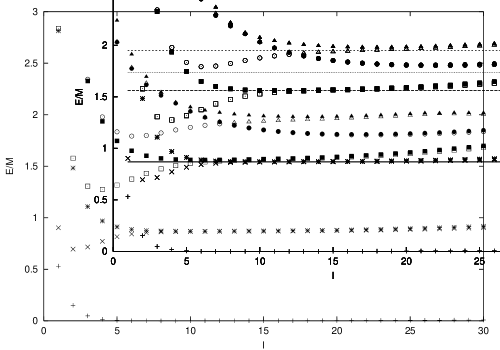
Figure 5: Breather masses in the 2-folded model with $p=2/7$

Denoting the kink of rapidity $\theta$, interpolating between the vacuum $\alpha$ at $x\rightarrow-\infty$ and $\beta$ at $x\rightarrow\infty$ by $K_{\alpha\beta}(\theta)$, we let the amplitude

$$S_{\alpha\beta}^{\gamma\delta}(\theta_{12})$$

describe the process

$$K_{\alpha\gamma}(\theta_{1})+K_{\gamma\beta}(\theta_{2})\rightarrow K_{\alpha\delta}(\theta_{2})+K_{\delta\beta}(\theta_{1})\,,$$

where $\theta_{1}>\theta_{2}$ and $\theta_{12}=\theta_{1}-\theta_{2}$. Labelling the vacua by $\alpha=0,1\dots,k-1$ the model $\mathrm{SG}(\beta,k)$ has kinks $K_{\alpha\beta}$ with $|\alpha-\beta|=1$ (or $k-1$). It is easy to describe the $S$-matrices of these kinks [4]: using the ${\mathbb{Z}}_{k}$ symmetry as well as time reversal and parity invariance one can show that every nonvanishing kink-kink amplitude is equal to one of the following three amplitudes: $S_{\alpha\alpha+2}^{\alpha+1\alpha+1}(\theta_{12})$, $S_{\alpha\alpha}^{\alpha+1\alpha+1}(\theta_{12})$, $S_{\alpha\alpha}^{\alpha+1\alpha-1}(\theta_{12})$, where $\alpha\pm 1$, $\alpha+2$ are understood mod $k$. These ($\alpha$ independent) amplitudes are also independent of the global properties of $\varphi$ and thus they should be equal to the soliton-soliton ($S_{ss}(\theta)$), antisoliton-soliton reflection ($S_{R}(\theta)$), and antisoliton-soliton transmission ($S_{T}(\theta)$) amplitudes, respectively, of the ordinary SG model. To compute multi-kink energy levels we need the explicit form of $S_{ss}(\theta)$:

$$S_{ss}(\theta)=-e^{i\delta(\theta)}\,,\quad\delta(\theta)=\int^{\infty}_{0}\frac{d\omega}{\omega}\frac{\sin(\theta\omega)\sinh\left(\frac{\pi}{2}\omega(p-1)\right)}{\cosh\left(\frac{\pi}{2}\omega\right)\sinh\left(\frac{\pi}{2}\omega p\right)}\>.$$

In a completely analogous way one obtains that the $S_{n}^{(m)}(\theta_{12})$ $S$-matrix, which describes the possible breather-kink scatterings

$$B^{(m)}_{n}(\theta_{1})+K_{n,n+1}(\theta_{2})\to K_{n,n+1}(\theta_{2})+B^{(m)}_{n+1}(\theta_{1})\,,\quad\theta_{1}>\theta_{2}$$

coincides with the breather-soliton $S_{s}^{(m)}(\theta_{12})$ $S$-matrix of the SG model [17]:

$$S^{(m)}_{s}(\theta)=\frac{\sinh\theta+i\cos\frac{\pi mp}{2}}{\sinh\theta-i\cos\frac{\pi mp}{2}}\prod^{m-1}_{l=1}\frac{\sin^{2}\left(\frac{m-2l}{2}\pi p-\frac{p}{4}+i\frac{\theta}{2}\right)}{\sin^{2}\left(\frac{m-2l}{2}\pi p-\frac{p}{4}-i\frac{\theta}{2}\right)}\,.$$ (5.5)

In finite volume, when the boundary condition (2.3) is imposed the single kink particles disappear from the theory and they survive only as the building block constituents of the multi-kink state with integer topological charge. On the other hand the breather particles $B_{n}^{(m)}$ are there even in finite volume, as they are consistent with (2.3).

5.3 The Bethe–Yang equations

To make a comparison with the TCSA results we need the multi-particle energy levels as functions of $L$. While it is possible to get them directly in the NLIE formalism, we shall use a simpler (and approximate) method which can be shown to give equivalent results for large volume ($ML\gg 1$) but which has a clear interpretation in terms of the spectrum of the model as it was described above.

In an integrable theory particle number is conserved, thus the concept of $N$ particle state with any fixed $N$ is well defined, at least for $L\gg M^{-1}$ when most of the time the particles are far from each other. First we consider the ‘pure’ multi-kink states and envisage the $N$-kink energy eigenstate in a large volume as a stationary scattering state, characterized by the set of (conserved) rapidities $\vec{\theta}=\{\theta_{1},\ldots,\theta_{N}\}$. Any $N$-kink stationary wavefunction can be expanded using the independent allowed $N$-kink in-states (the number of which we denote by $d_{N}$)

$$\left|K_{n_{1}n_{2}}(\theta_{1})K_{n_{2}n_{3}}(\theta_{2})\ldots K_{n_{N}n_{1}}(\theta_{N})\right\rangle\>,\quad\theta_{1}>\theta_{2}>\ldots>\theta_{N}$$

as basis, and let $\psi^{\mathbf{n}}(\vec{\theta})$ ($\mathbf{n}=(n_{1}\ldots n_{N})$) denote its components with respect to this basis. Then, as a consequence of the periodic boundary conditions $\psi^{\mathbf{n}}(\vec{\theta})$ must satisfy the following Bethe–Yang equations (at least if all particles have the same mass):

$$e^{iML\sinh\theta_{j}}\sum_{\mathbf{n}}T_{j}(\vec{\theta})^{\mathbf{m}}_{\mathbf{n}}\psi^{\mathbf{n}}(\vec{\theta})=-\psi^{\mathbf{m}}(\vec{\theta})\,,\quad j=1,\ldots,N\,,$$ (5.6)

where $T_{j}(\vec{\theta})$ is the $N$ particle transfer matrix [4]:

$$T_{j}(\vec{\theta})^{\mathbf{m}}_{\mathbf{n}}=\prod^{N}_{i=1}S_{m_{i}n_{i+1}}^{n_{i}m_{i+1}}\left(\theta_{j}-\theta_{i}\right)\>.$$

For a given $L$ eqns. (5.6) have solutions only for some special $\theta_{j}$, and the total energy and momentum of the system in a state characterized by these solutions are given by

$$E=\sum^{N}_{j=1}M\cosh\theta_{j}\>,\quad P=\sum^{N}_{j=1}M\sinh\theta_{j}\,.$$ (5.7)

Note however, that while this expression for $P$ is exact even for finite $L$, the one for $E$ is only approximate, as we neglect the ‘tunnelling’ and ‘off-shell’ corrections.

It is straightforward to use this formalism to obtain the energy levels of pure multi-kink states in the $Q=n$ ($n\geq 1$) sector of $\mathrm{SG}(\beta,k)$. It is natural to assume, that the lowest energy levels in this sector correspond to states with the smallest possible number of particles. The states with lowest number of particles compatible with the boundary condition and the topological charge being $n$ contain $N=k\cdot n$ kinks and no breathers or antikinks. Since the sequence of kinks in these states is necessarily fixed, we have, independently of $n$, only $k$ different basis vectors in this subspace, i.e. $d_{N}=k$. The basis vectors can be chosen as

$$\left|\psi_{0,1,\ldots,k-1}\left(\theta_{1},\ldots,\theta_{k\cdot n}\right)\right\rangle = \left|K_{01}\left(\theta_{1}\right)\ldots K_{k-1,0}\left(\theta_{k}\right)K_{01}\left(\theta_{k+1}\right)\ldots K_{k-1,0}\left(\theta_{k\cdot n}\right)\right\rangle$$

$$\left|\psi_{k-1,0,\ldots,k-2}\left(\theta_{1},\ldots,\theta_{k\cdot n}\right)\right\rangle = \left|K_{k-1,0}\left(\theta_{2}\right)K_{01}\left(\theta_{1}\right)\ldots\right.$$

$$\left.K_{k-2,k-1}\left(\theta_{k}\right)K_{k-1,0}\left(\theta_{k+1}\right)\ldots K_{k-2,k-1}\left(\theta_{k\cdot n}\right)\right\rangle$$

$$\left|\psi_{1,\ldots,k-1,0}\left(\theta_{1},\ldots,\theta_{k\cdot n}\right)\right\rangle = \left|K_{1,2}\left(\theta_{1}\right)\ldots K_{0,1}\left(\theta_{k}\right)K_{1,2}\left(\theta_{k+1}\right)\ldots K_{0,1}\left(\theta_{k\cdot n}\right)\right\rangle\,,$$ (5.8)

where $\theta_{1}>\theta_{2}>\ldots>\theta_{k\cdot n}$. Using the explicit form of the transfer matrix and the identification of the various $S_{\alpha\beta}^{\gamma\delta}$ elements with the SG soliton-soliton $S$-matrix $S_{ss}(\theta)$, the Bethe–Yang equations can finally be written in the following form:

$$e^{iML\sinh\theta_{i}}\prod_{j\neq i}^{k\cdot n}e^{i\delta\left(\theta_{i}-\theta_{j}\right)}(-1)^{k\cdot n}T_{k}\psi=-\psi\>,\quad i=1,\ldots,k\cdot n\\ ,,$$

where $\psi$ is a column vector made of the $\psi^{\mathbf{n}}$ coefficients of the basis vectors in eqn. (5.8) and the $k\times k$ matrix $T_{k}$

$$T_{k}=\left(\begin{array}[]{cccc}0&\ldots&&1\\ 1&\ldots&&0\\ 0&1&\ldots&0\\ \vdots&&&\\ 0&\ldots&1&0\end{array}\right)$$

describes a cyclic permutation generating ${\mathbb{Z}}_{k}$. The eigenvectors $\psi_{m}$ belonging to the various eigenvalues ($e^{i\frac{2}{\pi}m/k}$, $m=0,\dots,k-1$) of $T_{k}$ carry the different inequivalent irreducible representations of ${\mathbb{Z}}_{k}$. Choosing the $m$-th eigenvalue of $T_{k}$ and introducing the dimensionless variable $l=ML$ gives rise to the following Bethe–Yang equations

$$l\sinh\theta_{i}+\sum_{j\neq i}\delta(\theta_{i}-\theta_{j})=2\pi\left(\hat{N}_{i}-\frac{m}{k}\right)\>,i=1,\ldots k\cdot n\,,$$ (5.9)

where $\hat{N}_{i}\in{\mathbb{Z}}+1/2$ for $k\cdot n$ even and $\hat{N}_{i}\in{\mathbb{Z}}$ for $k\cdot n$ odd, and as a result of $S_{ss}(0)=-1$ we must have $\hat{N}_{i}\neq\hat{N}_{j}$ for $i\neq j$. The total momentum carried by a solution of (5.9) is determined solely in terms of the $\hat{N}_{i}$:

$$\frac{P}{M}=\frac{2\pi}{l}\left(\sum_{i}\hat{N}_{i}-m\cdot n\right)\,.$$

The simplest possibility—and the one we investigated by TCSA—is when the total (CM) momentum vanishes, $P=0$. Please note that as a consequence of $\delta(-\theta)=-\delta(\theta)$ and $e^{i2\pi(k-m)/k}=e^{-i2\pi m/k}$ the Bethe–Yang equations guarantee that the $P=0$ states $(\psi_{m},\psi_{k-m})$, which carry complex conjugate representations of ${\mathbb{D}}_{k}$, are degenerate in energy.

It is also possible to arrive at this result directly from the NLIE discussed in Section 3. In the infrared limit $ML\gg 1$ the integral term in the NLIE (3.1) becomes negligible and for a state with $k\cdot n$ holes the equation simplifies to

$$Z(\theta)=\vartheta+l\sinh\theta+\sum^{k\cdot n}_{j=1}\chi(\theta-\theta_{j})\>.$$

Observing that $\chi(\theta)\equiv\delta(\theta)$ and remembering that the allowed values of $\vartheta$ (3.8) are exactly equivalent to selecting

$$\vartheta_{m}=2\pi\frac{m}{k}\>,\quad k=0,\ldots,m-1\>,$$

the Bethe quantization rules reduce to eqn. (5.9) while the energy/momentum formulas turn into (5.7). Note that the quantization rule (3.7) which selects the local operator algebra ${\cal A}_{b}$ from (2.2) is exactly the one observed above for the $\hat{N}_{i}$: for $k\cdot n$ even it assigns half-integer, while for $k\cdot n$ odd integer Bethe quantum numbers $I_{i}$. We remark here that in general the large volume limit of the NLIE coincides with the Bethe–Yang equations (5.6) in their scalar form, i.e. evaluated on the eigenvectors of the transfer matrix $T^{\mathbf{m}}_{\mathbf{n}}(\vec{\theta})$.

5.3.1 Comparison with the TCSA data

To compare with the TCSA results we consider a few sectors of the models with $k=2$ and $k=3$ in more detail. The simplest of them is the $Q=1$ sector of $\mathrm{SG}(\beta,2)$. In this case $\psi_{0}$ describes the symmetric and $\psi_{1}$ the antisymmetric wave functions of $K_{01}$ and $K_{10}$, the latter one being allowed as the two kinks are different (bosonic) particles. $P=0$ implies in this case that $\theta_{1}=-\theta_{2}=\theta$ and (5.9) simplify to

$$l\sinh\theta+\delta(2\theta)=2\pi\left\{\begin{array}[]{ll}N_{0}\in{\mathbb{Z}}+\frac{1}{2}\,,&m=0\,,\\ N_{1}\in{\mathbb{Z}}\setminus\{0\}\,,&m=1\,.\end{array}\right.$$ (5.10)

From this equation $\theta=\theta(l,N_{m})$ can be determined using e.g. an iterative procedure, or alternatively the volume dependence of the $2$-kink energy levels can be given in parametric form as

$$\left(l,\frac{E}{M}\right)(\theta)=\left(\frac{2\pi N_{m}-\delta(2\theta)}{\sinh\theta}\,,\,2\cosh\theta\right)\,.$$ (5.11)

This makes it clear that on the $(l,E/M)$ plane the $2$-particle lines cannot intersect each other for $0<l<\infty$. These findings make it possible to distinguish clearly between the solitons of sine–Gordon theory and the kinks in the 2-folded model, i.e. to argue that the $Q=2$ sector of $\mathrm{SG}(\beta,1)$ (denoted as $SG(\beta,1)_{2}$) is different from the $Q=1$ sector of $\mathrm{SG}(\beta,2)$ ($SG(\beta,2)_{1}$). Indeed it is straightforward to derive the Bethe–Yang equations for the pure 2-soliton states in $\mathrm{SG}(\beta,1)_{2}$; since these solitons are identical particles these Bethe–Yang equations are given by the first line in eqn. (5.10). Therefore the number of 2-soliton states in $\mathrm{SG}(\beta,1)_{2}$ is half the number of the 2-kink ones in $\mathrm{SG}(\beta,2)_{1}$. On Fig. 6 the continuous lines are given by the interpolated TCSA data obtained in $\mathrm{SG}(\beta,2)_{1}$ with $p=2/7$, while the dots represent the TCSA data obtained in $\mathrm{SG}(\beta,1)_{2}$; they clearly correspond to every second line only.

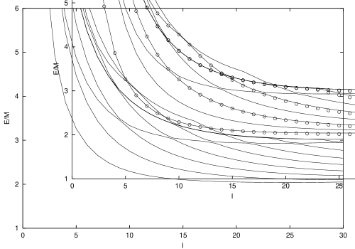
Figure 6: Comparison of the spectra of $\mathrm{SG}\left(\beta=\frac{4}{3}\sqrt{\pi},2\right)_{1}$ and $\mathrm{SG}\left(\beta=\frac{4}{3}\sqrt{\pi},1\right)_{2}$

Figure 7: The full spectrum and the predictions for $\mathrm{SG}\left(\beta=\frac{4}{3}\sqrt{\pi},2\right)_{1}$

On Fig. 7 the continuous lines depending on one quantum number only are given by eqn. (5.10) and the dots now correspond to the TCSA data in $\mathrm{SG}(\beta,2)_{1}$. On this figure we find data lines that cannot be interpreted as pure $2$-kink states, as they apparently do intersect some of the other lines. Since the large $l$ behaviour of these lines is compatible with $E\rightarrow 2M+M_{1}$ for $l\rightarrow\infty$, it is natural to try to interpret them as describing $3$-particle states containing one ‘first’ ($m=1$) breather in addition to the two kinks. Since $M_{1}\neq M$ the transfer matrix formalism worked out in [4] does not apply directly. Nevertheless following the original line of thought, namely by ‘commuting around’ any of the particles using the appropriate $S$-matrices one can derive the Bethe–Yang equations for the stationary scattering states.

Deleting the sequential or ‘upper’ $(m)$ index of the breathers (since we consider only the first one) but keeping their ‘vacuum’ index the basis vectors in this $3$-particle subspace can be chosen as

$$\psi^{01\mathrm{h}} = \left|K_{01}\left(\theta_{1}\right)K_{10}\left(\theta_{2}\right)B_{0}\left(\theta_{3}\right)\right\rangle$$

$$\psi^{10\mathrm{h}} = \left|K_{10}\left(\theta_{1}\right)K_{01}\left(\theta_{2}\right)B_{1}\left(\theta_{3}\right)\right\rangle\,,\quad\theta_{1}>\theta_{2}>\theta_{3}\>,$$

plus $4$ other states corresponding to the breathers being ‘in the middle’ or in the ‘front’. (The index $\mathrm{h}$ signals that the breathers are the last). Introducing the notation $S_{s}^{(1)}(\theta)=-e^{i\alpha(\theta)}$, $M_{1}L=ml$ and $\psi^{\pm}=\frac{1}{\sqrt{2}}(\psi^{01\mathrm{h}}\pm\psi^{10\mathrm{h}})$, one can convert the Bethe–Yang equations derived by the ‘commuting around’ procedure into the following form:

$$l\sinh\theta_{1}+\delta(\theta_{1}-\theta_{2})+\alpha(\theta_{1}-\theta_{3}) = 2\pi N_{1}^{\gamma}$$ (5.12)

$$l\sinh\theta_{2}+\delta(\theta_{2}-\theta_{1})+\alpha(\theta_{2}-\theta_{3}) = 2\pi N_{2}^{\gamma}$$ (5.13)

$$ml\sinh\theta_{3}+\alpha(\theta_{3}-\theta_{1})+\alpha(\theta_{3}-\theta_{2}) = 2\pi K^{\gamma},$$ (5.14)

where $\gamma=\pm$, $N_{1,2}^{+}\in{\mathbb{Z}}$, $N_{1,2}^{-}\in{\mathbb{Z}}+1/2$, $K^{\gamma}\in{\mathbb{Z}}$. Once again, an equivalent system of equations can be derived from the NLIE in the $ML\gg 1$ (infrared) region.

In the $P=0$ system there are solutions with the breather at rest and the two kinks moving in opposite directions: $K^{\gamma}=0=\theta_{3}$, $N_{2}^{\gamma}=-N_{1}^{\gamma}$ $\theta_{2}=-\theta_{1}$. Then the (5.12–5.14) system simplifies to the single equation

$$l\sinh\theta_{1}+\delta(2\theta_{1})+\alpha(\theta_{1})=2\pi N_{1}^{\gamma},$$ (5.15)

which admits the parametric solution

$$\left(l,\frac{E}{M}\right)(\theta)=\left(\frac{2\pi N_{1}^{\gamma}-\delta(2\theta_{1})-\alpha(\theta_{1})}{\sinh\theta_{1}},2\cosh\theta_{1}+m\right).$$ (5.16)

It is easy to understand how the $N_{1}^{-}=-N_{2}^{-}=1/2$, $K^{-}=0$ state tends to the $N_{1}=1$ $2$-kink state (eqn. (5.10)) in the UV limit: in this limit $\alpha(\theta)\rightarrow-\pi$ and this effectively converts the $1/2$ on the right hand side of (5.15) into $1$. The lines depending on three quantum numbers on Fig. 7 correspond to the first two possibilities given by eqn. (5.15), and the agreement with the TCSA data is excellent. Note also that the line with $N_{1}^{+}=N_{2}^{+}=1$, $K^{+}=0$ is also present in $\mathrm{SG}(\beta,1)_{2}$, consistently with the data on Fig. 6.

The $Q=1$ sector of $\mathrm{SG}(\beta,3)$ is interesting, as the representations belonging to $m=1$ and $m=2\equiv-1$ are complex conjugate ones. The Bethe–Yang equations in this case take the form

$$l\sinh\theta_{i}+\sum_{j\neq i}^{3}\delta\left(\theta_{i}-\theta_{j}\right)=2\pi\left\{\begin{array}[]{ll}N^{(i)}_{0}\in{\mathbb{Z}}\,,&m=0\,,\\ N^{(i)}_{\pm 1}\in{\mathbb{Z}}\pm\frac{1}{3}\,,&m=\pm 1\,,\end{array}\right.\>\mathrm{where}\>\begin{array}[]{l}i=1,2,3\ \mathrm{and}\\ N_{m}^{(i)}\neq N_{m}^{(j)}\mathrm{\>}\mathrm{for}\>i\neq j\end{array}\,.$$

For the symmetric states (i.e. when $m=0$) with $P=0$ there are special solutions with $\theta_{3}=-\theta_{1}$, $\theta_{2}=0$ (when $N^{3}_{0}=-N^{1}_{0}=-N$, $N^{2}_{0}=0$); and for them the volume dependence of the energy levels can be given in parametric form similar to eqn. (5.11), but apart from these special cases we have to rely on numerical procedures to get $\frac{E}{M}(l,N^{i}_{m})$. On Fig. 8, for $p=2/7$, we show how well the predictions of these Bethe–Yang equations describe the TCSA data, regarding both the degeneracies and the volume dependence.

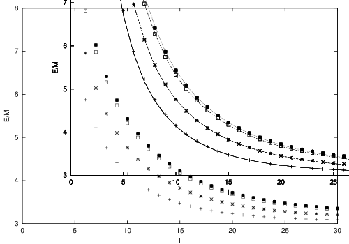
Figure 8: Bethe–Yang curves and TCSA data for $\mathrm{SG}\left(\beta=\frac{4}{3}\sqrt{\pi},3\right)_{1}$

6 Vacuum expectation values of local fields

In this section we analyze the vacuum expectation values of exponential fields. Some time ago an explicit expression was given for this quantity by Lukyanov and Zamolodchikov [8]. Here we compare this prediction with the data extracted from TCSA, and by doing so we give further evidence that everything which in sine–Gordon theory follows only from the local properties of the scalar field and the Lagrangian remains true in the $k$-folded model as well.

6.1 Symmetries and vacuum expectation values

In this subsection we will isolate the independent amplitudes which characterize the vacuum expectation values of exponential fields in $\mathrm{SG}(\beta,k)$:

$$\left\langle\vartheta_{n}\right|V_{m}\left|\vartheta_{r}\right\rangle\,,\quad V_{m}=V_{(m,0)}=\exp\left({i\beta}\frac{m}{k}\varphi\right)\>.$$

Our considerations will be valid for any value of the volume $L$.

As a consequence of the action of $T$ on the vacua $\left|\vartheta_{n}\right\rangle$ (2.10) and on the local fields $V_{m}$ (2.14) we have

$$\left\langle\vartheta_{n}\right|V_{m}\left|\vartheta_{r}\right\rangle=A_{m}(r)\delta_{n,m+r}\,,\quad\left\langle n\right|V_{m}\left|r\right\rangle=B_{m}(r-n)e^{\frac{2\pi i}{k}mn}\,,$$ (6.1)

where $A_{m}(r)$ are certain (unknown) amplitudes and

$$B_{m}(r)=\left\langle 0\right|V_{m}\left|r\right\rangle=\frac{1}{k}\sum^{k-1}_{n=0}e^{-\frac{2\pi i}{k}nr}A_{m}(n)\,.$$ (6.2)

Reality of the field $\varphi$ yields

$$V^{\dagger}_{m}=V_{-m}$$

and so

$$B_{m}(r)^{*}=e^{\frac{2\pi i}{k}rm}B_{-m}(-r)\,.$$

The transformation properties of the field $\varphi$ under $S$ imply

$$B_{m}(r)=B_{-m}(-r)\,.$$

This allows us to determine the phase of the amplitude $B_{m}(r)$ up to a sign:

$$B_{m}(r)=e^{\frac{\pi i}{k}rm}F_{m}(r)\,,\quad F_{m}(r)\in{\mathbb{R}}\,.$$ (6.3)

It turns out that the real amplitudes $F_{m}(r)$ are not all independent. Indeed, as it was already remarked in subsection 2.3, in the usual basis (2.21) of the (ultraviolet) free boson Hilbert space all the $V_{m}$ have real matrix elements. Therefore the Hamiltonian (2.8) as a matrix is real and symmetric, and as a consequence all its eigenvectors have real components. This implies

$$\left\langle\vartheta_{n}\right|V_{m}\left|\vartheta_{r}\right\rangle\in{\mathbb{R}}$$

and as a result

$$F_{m}(r)=(-1)^{m}F_{m}(k-r)\,,\quad r=1,\ldots,k-1\,.$$ (6.4)

Note that there is no constraint on $F_{m}(0)=\left\langle 0\right|V_{m}\left|0\right\rangle$. The vacuum expectation values can therefore be characterized by the independent amplitudes

$$F_{m}(r)\,,\quad r=0,\ldots,\left[\frac{k}{2}\right]$$ (6.5)

all of which are real.

6.2 The Lukyanov–Zamolodchikov formula

In [8] Lukyanov and Zamolodchikov proposed an exact formula for the vacuum expectation values of exponential fields in the ordinary sine–Gordon model in infinite volume. Here we briefly recall their result. We normalize the exponential fields so that the short distance asymptotics of the non-vanishing two-point functions reads

$$\left\langle 0\right|e^{ia\varphi(x)}e^{-ia\varphi(y)}\left|0\right\rangle=\frac{1}{|x-y|^{2\Delta_{a}}}\,,$$

where $\Delta_{a}=\frac{a^{2}}{8\pi}$ is the conformal weight of $e^{ia\varphi(x)}$, and $\left|0\right\rangle$ denotes the state $\left|n\right\rangle$ for $n=0$ (see eqn. (2.5)). Let us define

$${\cal G}(a)=\left\langle 0\right|e^{ia\varphi(x)}\left|0\right\rangle\,.$$

The authors of [8] conjecture

$${\cal G}(a) = \left[\frac{M\sqrt{\pi}\Gamma\left(\frac{p+1}{2}\right)}{2\Gamma\left(\frac{p}{2}\right)}\right]^{\frac{a^{2}}{4\pi}}\times$$ (6.6)

$$\exp\left\{\int^{\infty}_{0}\frac{\mathrm{d}t}{t}\left[\frac{\sinh^{2}\left(\frac{a\beta}{4\pi}t\right)}{2\sinh\left(\frac{p}{p+1}t\right)\sinh(t)\cosh\left(\frac{1}{p+1}t\right)}-\frac{a^{2}}{4\pi}e^{-2t}\right]\right\}\,,$$

which is valid for

$$\beta^{2}<8\pi\quad{\mathrm{and}}\quad\left|\Re e\,a\beta\right|<4\pi\,,$$ (6.7)

and where $M$ is the soliton (kink) mass. Recalling now our basic idea, namely that everything which depends only on the local properties of $\varphi$ and the SG Lagrangian also holds for the $k$-folded model $\mathrm{SG}(\beta,k)$, we can identify ${\cal G}(a)$ and $F_{m}(0)$:

$${\cal G}\left(\frac{m\beta}{k}\right)=F_{m}(0)\quad\mathrm{when}\quad l=ML=\infty.$$

The TCSA data allow us to extract at finite $l$ the expectation value of $e^{ia\varphi(w,\bar{w})}|_{|w|=1}$ (where $w=e^{\frac{2\pi}{L}z}$ is the map from the cylinder to the plane) in the ground states found by the numerical diagonalization, i.e. we can measure $A_{m}(n)$ as functions of $l$, $A_{m}(n)[l]$. Thus introducing the dimensionless function $g(a)=M^{-2\Delta_{a}}{\cal G}(a)$ we obtain for finite $l$:

$$F_{m}(0)[l]=\frac{1}{k}\sum\limits_{n=0}^{k-1}A_{m}(n)[l]=\frac{l^{2\Delta_{a}}}{(2\pi)^{2\Delta_{a}}}g(a)N(l)\,,\quad a=\frac{m\beta}{k}\,,$$ (6.8)

where $N(l)$ is a finite size “correction” factor of which we know $N(l)\rightarrow 1+{\cal O}(e^{-l})$ for $l\rightarrow\infty$.

The amplitudes $F_{m}(r)$ are in general not known for $r\neq 0$. However, one can derive their leading behaviour for large volume using the following consideration. First note that the matrix elements

$$\left\langle 0\right|V_{m}\left|r\right\rangle$$

vanish in infinite volume since there is a super-selection rule making the vacua $\left|n\right\rangle$ lie in physically disconnected Hilbert spaces with no local operators connecting them. It is clear that in finite volume the non-vanishing contribution to these matrix elements comes from the vacuum tunnelling described by instanton effects, whose magnitude we calculated for large $l$ in section 4. Therefore we expect

$$\left\langle 0\right|V_{m}\left|r\right\rangle\sim e^{-l}\quad\mathrm{when}\quad l\gg 1\quad\mathrm{and}\quad r\neq 0\,.$$

6.3 Comparison to TCSA

We tested the Lukyanov–Zamolodchikov formula in a 3-folded model with $p=2/7$. Using the eigenvectors belonging to the three ground states found by the TCSA algorithm we determined numerically the various amplitudes $A_{m}(n)[l]$ for all the values of $m$ ($m=1,\dots,5$) satisfying the conditions (6.7). Then, recalling eqn. (6.8), we plotted $F_{m}(0)[l]l^{-2\Delta_{m}}$ where

$$2\Delta_{m}=\frac{m^{2}\beta^{2}}{4k^{2}\pi}$$

as a function of $l$. The result is shown on Fig. 9, where the horizontal lines correspond to

$$(2\pi)^{-2\Delta_{m}}g\left(\frac{m\beta}{k}\right)\,.$$

The agreement between the measured values and the predicted ones is very good, though for higher values of $m$ the data are somewhat below the horizontal lines indicating that the TCSA data should be extrapolated as in the discussion that follows.

Figure 9: TCSA data and the Lukyanov–Zamolodchikov prediction

Figure 10: The decay of $F_{1}(1)[l]$

\psfrag{VEV}{$\mathrm{F}_{1}(0)/\mathrm{l}^{2\Delta_{1}}$}\includegraphics{VEVfit.eps}

Figure 11: Comparing TCSA with the semiclassical and full quantum formulae

The 3-folded model provides a good laboratory as it makes possible to extract $F_{m}(1)[l]$ from the data as well. The result $F_{1}(1)[l]$ can be seen on a semilogarithmic plot on Fig. 10. Clearly this behaviour is consistent with the expected exponential fall-off.

The exact expression for ${\cal G}(a)$ was obtained in [8] by a clever interpolation between various limits, where the corresponding expressions were known from other sources. One important such limit was the semiclassical one. Since our numerical study is for $p<1$, we investigated whether using our data one can make a distinction between the exact and semiclassical expressions of [8], i.e. whether one can justify the exact or merely the semiclassical formula.

We carried this out by zooming in on the vicinity of the uppermost ($m=1$) line on Fig. 9, and the results are compiled on Fig. 11. Here the upper/lower horizontal line corresponds to a $g(a,\beta)$ obtained by the exact/semiclassical expressions in [8], and the TCSA data displayed were taken at four different $E_{\mathrm{cut}}$ values. At each fixed $l$ the data apparently converge monotonously with increasing $E_{\mathrm{cut}}$. The validity of the exact expression over the semiclassical one is supported by the fact that these monotonously convergent data exceed the semiclassical expression in a certain range, while they always stay below the exact one. To strengthen this conclusion, at each fixed $l$, we extrapolated the data by fitting their $E_{\mathrm{cut}}$ dependence with an expression

$$a(l)\frac{E_{\mathrm{cut}}^{2(2-h)}+c(l)}{E_{\mathrm{cut}}^{2(2-h)}+b(l)}\,,$$

and the extrapolated points on Fig. 11 correspond to the coefficients $a(l)$. These extrapolated points show a monotonously increasing behaviour in $l$ and they significantly exceed the semiclassical expression while always stay below the exact one. In the final step, recalling eqn. (6.8), we fitted the extrapolated points by $A-Be^{-l}/l$, where $e^{-l}$ is motivated by the instanton contribution, and the $l^{-1}$ by the fluctuation determinant without a zero mode. This ‘instanton fit’ describes the extrapolated data with a very small variance, and though the $A$ obtained this way is somewhat smaller than the exact expression, it is much closer to the exact than to the semiclassical one. To sum up, we can say that our data indeed favour the exact expression of [8] over the semiclassical one.

We remark that a similar calculation of vacuum expectation values from TCSA was performed in [18] for the case of $\Phi_{(1,3)}$ perturbations of Virasoro minimal models. These models are restrictions of sine–Gordon theory at rational values of $p$ and as a consequence one can derive a formula for the vacuum expectation values of local fields starting from (6.6) [8]. Similarly to our case, they find that the respective formula agrees with the TCSA results. In contrast to their approach, however, we checked the prediction (6.6) directly in the case of sine–Gordon theory.

There is another important implication of this result. The Lukyanov–Zamolodchikov conjecture for the vacuum expectation values of local fields is connected to (and can be derived from) the conjecture for the so-called Liouville reflection factor [19, 20]. The above verification of the formula (6.6) therefore lends an indirect support to the conjectured expression for the reflection factor and considerations based on it.

7 Conclusions

In this paper we investigated the $k$-folded sine–Gordon model $\mathrm{SG}(\beta,k)$ in finite volume. The aim of this study is to give support to the idea that the $k$-folded boundary conditions which make $\mathrm{SG}(\beta,k)$ different from the ordinary sine–Gordon theory do indeed preserve the integrability of the model, while changing the spectrum in a well defined manner.

We analyzed three major problems in some detail and showed in all of them, that the consequences one can draw from this expectation are indeed correct. In particular we found that the leading part of the split in the ground state energy levels, for which the NLIE and the instanton calculus gave identical results, does indeed coincide with the numerical data obtained by using TCSA. Furthermore, we provided evidence that the $k$ dependent degeneracies and the volume dependence of the multi-particle energy levels can indeed be described by the formalism of [4], thus indirectly we verified the conjectured $S$-matrices. Last but not least we showed that the vacuum expectation value of the exponential field can be measured in the $k$ folded model and we gave evidence supporting the validity of the formula proposed in [8].

Acknowledgements

G. Takács would like to thank G. Watts for useful discussions. G. T. is supported by a PPARC (UK) postdoctoral fellowship, while Z. B. by an OTKA (Hungary) postdoctoral fellowship D25517/97. This research was also supported in part by the Hungarian Ministry of Education under FKFP 0178/1999 and the Hungarian National Science Fund (OTKA) T029802/99.

Appendix A Instanton calculus in finite volume

In this appendix we perform a standard instanton calculation based on the dilute instanton gas approximation, following the outlines of [21]. Here we shall work in a $k=\infty$ theory which means that we drop the identification of the field in (2.2). We will comment on this issue later.

A.1 The dilute instanton gas approximation

The Euclidean action of sine–Gordon theory is

$$S_{E}[\varphi]=\int^{\infty}_{-\infty}\mathrm{d}\tau\int^{L/2}_{-L/2}\mathrm{d}x\left(\frac{1}{2}\left(\partial_{\tau}\varphi\right)^{2}+\frac{1}{2}\left(\partial_{x}\varphi\right)^{2}+\frac{\mu^{2}_{0}}{\beta^{2}}\left(1-\cos\beta\varphi\right)\right)\,.$$ (A.1)

The equations of motion following from the action (A.1) admit the one-instanton solution

$$\varphi_{\mathrm{inst}}=\frac{4}{\beta}\arctan\exp\left(\mu_{0}\left(\tau-\tau_{0}\right)\right)$$ (A.2)

with action

$$S_{E}\left[\varphi_{\mathrm{inst}}\right]=\frac{8\mu_{0}}{\beta^{2}}L=M_{\mathrm{class}}L\,,$$ (A.3)

where $M_{\mathrm{class}}$ is the classical soliton mass. Using the usual rules of instanton calculus, the saddle-point evaluation of the Euclidean path integral yields the following result for the level splitting as a function of the twist angle $\vartheta$ labelling the energy eigenstates $|\vartheta\rangle$:

$$\Delta E(\vartheta)=-2\cos\left(\vartheta\right)\left|\frac{\det^{\prime}M}{\det M_{0}}\right|^{-1/2}\left(\frac{S_{E}\left[\varphi_{\mathrm{inst}}\right]}{2\pi}\right)^{1/2}e^{-S_{E}\left[\varphi_{\mathrm{inst}}\right]}\,,$$ (A.4)

where $M$ and $M_{0}$ are the operators

$$M=-\partial^{2}_{\tau}-\partial^{2}_{x}+V^{\prime\prime}\left(\varphi_{\mathrm{inst}}\right)\,,\quad M_{0}=-\partial^{2}_{\tau}-\partial^{2}_{x}+V^{\prime\prime}\left(0\right)$$ (A.5)

describing the fluctuations around the instanton to quadratic order, $\det^{\prime}M$ denotes the determinant of $M$ without its zero mode and the factor

$$\left(\frac{S_{E}\left[\varphi_{\mathrm{inst}}\right]}{2\pi}\right)^{1/2}$$ (A.6)

comes from the one translational zero mode $\tau_{0}$ of the instanton solution (A.2). The $\cos\vartheta$ dependence arises from Fourier transforming the dilute instanton gas summation according to the relation between the vacua $\left|n\right\rangle$ and $\left|\vartheta\right\rangle$:

$$\left|\vartheta\right\rangle=\sum^{\infty}_{n=-\infty}e^{in\vartheta}\left|n\right\rangle\>.$$ (A.7)

Here $\vartheta$ can take any value: the physically inequivalent choices are $-\pi<\vartheta\leq\pi$. For $\mathrm{SG}(\beta,k)$, the result of the dilute instanton gas calculation is similar to (A.4) with the only difference that $\vartheta$ can only take the discrete values

$$\vartheta_{n}=\frac{2\pi n}{k}\>\bmod\>2\pi\,.$$

A.2 The heat kernel representation for the determinant

Let us define the heat kernel for a positive hermitian operator $A$ in the following way:

$$K_{t}(A)=\mathrm{Tr}\,e^{-tA}\,,$$ (A.8)

from which the determinant can be reconstructed:

$$\log\det\mathrm{A}=\mathrm{Tr}\log A=-\int^{\infty}_{0}\frac{\mathrm{d}t}{t}K_{t}(A)\,.$$ (A.9)

As the determinant is divergent (the divergence comes from the lower end of the integration over $t$), we shall compute the difference

$$\tilde{K}_{t}(M)=K_{t}(M)-K_{t}\left(M_{0}\right)$$

using $\zeta$-function regularisation. We define the $\zeta$-function

$$\zeta(z,M)=\frac{1}{\Gamma(z)}\int^{\infty}_{0}\mathrm{d}t\ t^{z-1}\left(\tilde{K}_{t}(M)-1\right)\>.$$ (A.10)

Then the determinant can be expressed as

$$\left|\frac{\det^{\prime}M}{\det M_{0}}\right|^{-1/2}=\left.\exp\left(\frac{1}{2}\frac{d}{dz}\zeta(z,M)\right)\right|_{z=0}\>.$$ (A.11)

We can separate the $x$ and $\tau$ dependence and rewrite the heat kernel in the following form:

$$\tilde{K}_{t}(M) = K_{t}\left(-\partial^{2}_{x}\right)\left(K_{t}\left(Q\right)-K_{t}\left(Q_{0}\right)\right)\,,$$

$$Q = -\partial^{2}_{\tau}+\mu^{2}_{0}\left(1-\frac{2}{\cosh^{2}\left(\mu_{0}(\tau-\tau_{0})\right)}\right)\,,$$

$$Q_{0} = -\partial^{2}_{\tau}+\mu^{2}_{0}\,.$$

The heat kernels for the three operators that appear above are

$$K_{t}\left(-\partial^{2}_{x}\right) = \sum^{\infty}_{n=-\infty}e^{-\left(\frac{2\pi}{L}n\right)^{2}t}=\frac{L}{\sqrt{4\pi t}}\sum^{\infty}_{n=-\infty}e^{-\frac{n^{2}L^{2}}{4t}}\,,$$

$$K_{t}(Q) = 1+\int^{\infty}_{-\infty}\mathrm{d}p\rho(p)e^{-t\left(\mu^{2}_{0}+p^{2}\right)}\,,$$

$$K_{t}\left(Q_{0}\right) = \int^{\infty}_{-\infty}\mathrm{d}p\rho_{0}(p)e^{-t\left(\mu^{2}_{0}+p^{2}\right)}\,.$$ (A.12)

where $\rho$, $\rho_{0}$ are the spectral densities for the operators $Q$, $Q_{0}$ and the additive $1$ in $K_{t}(Q)$ comes from the zero mode.

A.3 Evaluation of the spectral densities

The spectral density of the operator

$$Q=-\partial^{2}_{\tau}+\mu^{2}_{0}\left(1-\frac{2}{\cosh^{2}\left(\mu_{0}\tau\right)}\right)$$ (A.13)

can be evaluated by solving the spectral problem:

$$-\Psi^{\prime\prime}-\frac{s(s+1)\mu^{2}_{0}}{\cosh^{2}\left(\mu_{0}\tau\right)}\Psi+\mu^{2}_{0}\Psi=\lambda\Psi\>,$$ (A.14)

where for our case $s=1$. This problem can be solved exactly by mapping the above equation to a hypergeometric one [22].

A.3.1 The discrete spectrum

The discrete spectrum of (A.14) corresponds to $0\leq\lambda<\mu^{2}_{0}$. The condition for square integrability reads

$$\sqrt{1-\frac{\lambda}{\mu^{2}_{0}}}-s=-n\,,\quad n\in{\mathbb{N}}\>.$$ (A.15)

For our case ($s=1$) the only solution of (A.15) is $n=0$ which corresponds to $\lambda=0$ i.e. exactly the unique zero mode of the operator $Q$ mentioned before. (The other possibility $n=1$ means $\lambda=\mu^{2}_{0}$ which is where the continuous spectrum starts.)

A.3.2 The continuous spectrum

The continuous spectrum covers the range $\mu^{2}_{0}\leq\lambda<\infty$. In this domain we define a solution with the following asymptotic property:

$$\Psi(\tau\to\infty)=e^{ip\tau}\,,\quad\lambda=\mu^{2}_{0}+p^{2}\,.$$

Then one can compute

$$\Psi(\tau\to-\infty)=\frac{\Gamma\left(\frac{ip}{\mu_{0}}\right)\Gamma\left(1-\frac{ip}{\mu_{0}}\right)}{\Gamma(-s)\Gamma(1+s)}e^{-ip\tau}+\frac{\Gamma\left(-\frac{ip}{\mu_{0}}\right)\Gamma\left(1-\frac{ip}{\mu_{0}}\right)}{\Gamma\left(-\frac{ip}{\mu_{0}}-s\right)\Gamma\left(1+s-\frac{ip}{\mu_{0}}\right)}e^{ip\tau}\,.$$ (A.16)

For $s\in{\mathbb{N}}$ the first term vanishes, which means that the potential is reflectionless. For $s=1$ we obtain

$$\Psi(\tau\to-\infty)=e^{i(p\tau+\delta(p))}\,,\quad e^{i\delta(p)}=\frac{ip+\mu_{0}}{ip-\mu_{0}}\,.$$ (A.17)

To get a well-defined spectral density, we must put the system in a large box of size $T$. Then periodic boundary condition on $\Psi$ implies

$$pT-\delta(p)=2\pi N\,,\quad N\in{\mathbb{Z}}.$$

For the size $T\to\infty$ the density of states with a given $p$ is

$$\rho(p)=\frac{1}{2\pi}\left(T-\frac{\partial\delta(p)}{\partial p}\right)\>,$$ (A.18)

which gives

$$\rho(p)=\frac{1}{2\pi}\left(T-\frac{2\mu_{0}}{p^{2}+\mu^{2}_{0}}\right)\>.$$ (A.19)

A similar, but much simpler reasoning for $Q_{0}$ yields

$$\rho_{0}(p)=\frac{T}{2\pi}\>,$$ (A.20)

so the divergent parts linear in $T$ drop out from the difference.

A.4 The instanton contribution

Substituting the results (A.19,A.20) into (A.12), the final result for the $\zeta$-regularized heat kernel (A.10) is

$$\zeta(z,M)=\zeta_{1}(z,M)+\zeta_{2}(z,M)+\zeta_{3}(z,M)\,,$$

where

$$\zeta_{1}(z,M) = \frac{1}{\Gamma(z)}\int^{\infty}_{0}\mathrm{d}t\,t^{z-1}L(4\pi t)^{-1/2}\left(K_{t}(Q)-K_{t}\left(Q_{0}\right)-1\right)\,,$$

$$\zeta_{2}(z,M) = \frac{1}{\Gamma(z)}\int^{\infty}_{0}\mathrm{d}t\,t^{z-1}\left(K_{t}\left(-\partial^{2}_{x}\right)-1\right)\,,$$

$$\zeta_{3}(z,M) = \frac{1}{\Gamma(z)}\int^{\infty}_{0}\mathrm{d}t\,t^{z-1}\left(K_{t}\left(-\partial^{2}_{x}\right)-L\left(4\pi t\right)^{-1/2}\right)\left(K_{t}(Q)-K_{t}\left(Q_{0}\right)-1\right)\,.$$

$\zeta_{1}$ and $\zeta_{3}$ correspond to renormalizing the classical soliton mass $M_{\mathrm{class}}$ to the quantum one. The interesting contribution to the determinant comes from the term $\zeta_{2}$ which gives

$$\left.\frac{\mathrm{d}\zeta_{2}(z,M)}{dz}\right|_{z=0} = -\log\frac{L^{2}}{4\pi}+\Gamma^{\prime}(1)-2+\int^{\infty}_{1}\frac{\mathrm{d}t}{t}\left(1+\sqrt{\frac{4\pi t}{L^{2}}}\right)\left(K_{t}\left(-\partial^{2}_{x}\right)-1\right)$$

$$= B-\log\frac{L^{2}}{4\pi}\>.$$

Numerical evaluation of the integral gives

$$2e^{\frac{B}{2}}=\frac{1}{\sqrt{\pi}}$$

to very high precision. Collecting all terms we get

$$\Delta E(\vartheta)=-M\sqrt{\frac{2}{\pi l}}e^{-l}\cos\vartheta\,.$$ (A.21)

References

- [1] A. B. Zamolodchikov, Adv. Stud. Pure Math. 19 (1989) 641.
- [2] S. Ghoshal and A. Zamolodchikov, Int. J. Mod. Phys. A9 (1994) 3841, hep-th/9306002.
- [3] J. A. Swieca Phys. Rev. D13 (1976) 312.
- [4] T. R. Klassen and E. Melzer, Nucl. Phys. B382 (1992) 441.
- [5] V. P. Yurov and Al. B. Zamolodchikov, Int. J. Mod. Phys. A6 (1991) 4557-4578.
-
[6]
A. Kl mper and P. A. Pearce, J. Stat. Phys.
64 (1991) 13;
A. Kl mper, M. Batchelor and P. A. Pearce, J. Phys. A24 (1991) 3111. -
[7]
C. Destri and H. J. De Vega, Phys. Rev. Lett.
69 (1992) 2313-2317.
C. Destri and H. J. De Vega, Nucl. Phys. B438 (1995) 413-454, hep-th/9407117. - [8] S. Lukyanov and A. B. Zamolodchikov, Nucl. Phys. B493 (1997) 571-587, hep-th/9611238.
- [9] T. R. Klassen and E. Melzer, Int. J. Mod. Phys.A8 (1993) 4131-4174, hep-th/9206114.
-
[10]
G. Feverati, F. Ravanini and G. Takács,
Nucl. Phys. B540 (1999) 543-586, hep-th/9805117.
G. Feverati, F. Ravanini and G. Takács, Phys. Lett. B444 (1998) 442-450, hep-th/9807160. - [11] Al. B. Zamolodchikov, Int. J. Mod. Phys. A10 (1995) 1125-1150.
-
[12]
Al. B. Zamolodchikov, Nucl. Phys.
B432 (1994) 427-456.
Al. B. Zamolodchikov, Phys. Lett. B335 (1994) 436-443. - [13] G. Feverati, F. Ravanini and G. Takács, Nucl. Phys. B570 (2000) 615-643, hep-th/9909031.
- [14] P. Fendley and H. Saleur: Massless Integrable Quantum Field Theories and Massless Scattering in (1+1)-Dimensions, hep-th/9310058. Lectures given at Summer School in High Energy Physics and Cosmology, Trieste, Italy, 1993. Published in Trieste HEP Cosmol. 1993, pp. 301-332. Also in Strings 1993, pp. 87-118.
- [15] D. Fioravanti, A. Mariottini, E. Quattrini and F. Ravanini, Phys. Lett. B390 (1997) 243-251, hep-th/9608091.
- [16] C. Destri and H. J. De Vega, Nucl. Phys. B504 (1997) 621-664, hep-th/9701107.
- [17] A. B. Zamolodchikov and Al. B. Zamolodchikov, Ann. Phys 120 (1979) 253.
- [18] R. Guida and N. Magnoli, Phys. Lett. B411 (1997) 127-133, hep-th/9706017.
- [19] A. B. Zamolodchikov and Al. B. Zamolodchikov, Nucl. Phys. B477 (1996) 577-605, hep-th/9506136.
- [20] V. Fateev, S. Lukyanov, A. B. Zamolodchikov and Al. B. Zamolodchikov, Phys. Lett. B406 (1997) 83-88, hep-th/9702190.
- [21] G. M nster, Nucl. Phys. B324 (1989) 630.
- [22] L. D. Landau and E. M. Lifshitz, Theoretical Physics III: Quantum Mechanics, Butterworth-Heinemann, 1997.