Scale Relativity in Cantorian $\cal E^{(\infty)}$ Space and Average Dimensions of Our World

Abstract

Cantorian fractal spacetime, a family member of von Neumann’s noncommutative geometry, is introduced as a geometry underlying a new relativity theory which is similar to the relation between general relativity and Riemannian geometry. Based on this model and the new relativity theory an ensemble distribution of all the dimensions of quantum spacetime is derived with the help of Fermat last theorem. The calculated average dimension is very close to the value of $4$+$\phi^{3}$ (where $\phi$ is the golden mean) obtained by El Naschie on the basis of a different approach. It is shown that within the framework of the new relativity the cosmological constant problem is nonexistent, since the Universe self-organizes and self-tunes according to the renormalization group (RG) flow with respect to a local scaling microscopic arrow of time. This implies that the world emerged as a result of a non-equilibrium process of self-organized critical phenomena launched by vacuum fluctuations in Cantorian fractal spacetime $\cal E^{\infty}$. It is shown that we are living in a metastable vacuum and are moving towards a fixed point ( $D_{av}$ = $4$ + $\phi^{3}$) of the RG. After reaching this point, a new phase transition will drive the universe to a quasi-crystal phase of the lower average dimension of $\phi^{3}$.

1 Introduction

Rephrasing I.Kant we can say that any physical theory should start from the first principles and assumptions based on intuition directly related to the existing physical phenomena, then proceed to the concepts, complete theory with a central idea , and crown it with the experimental verification and testable predictions. One of the best examples of this path is provided by the theory of relativity and quantum mechanics. Their further development spurred by the need to unite gravity and quantum mechanics resulted in the birth of the string theory.

During 30 years of its development the string theory demonstrated remarkable achievements in all but one respect: there is no direct way to verify its theoretical results. In addition, there is at least one ”thorny” question: why does the world we are living in appears to be $3+1$-dimensional? Up to now string theory could not produced a satisfactory answer. It seems that string theory ignored possible alternative basic assumptions which, as we will see later, could have produced a plausible answer: multi-fractality of spacetime, a possibility of spacetime dimensions ranging from negative dimensions to infinite ones,as in the $\cal E^{\infty}$ Cantorian theory of El Naschie [1] and the resolution-dependent character of physical laws as described for example by Nottale’s scale relativity [2].

One of the basic problem facing future developments of a successful physical theory is a description of the quantum ”reality” without introducing by hand a priori existing background. Interestingly enough, as one of the first steps in formulating the theoretical foundations of physics Newton disposed of this problem rather easily by simply introducing (almost at the very beginning of ”Principia”) the absolute space and time as entities ”which do not bear any relation to anything external”. It is clear that without an attendant background ( either not changing or changing rather slowly as compared to developing phenomena) any description of a physical theory looks impossible.

To formalize dynamics of physical phenomena we have to answer the following question: the dynamics with respect to what? For example, the Lagrangian of the string theory refers to the background of proper time (which is rather a vague notion since we have to have a physical device attached to a string and measuring time intervals which in turn are not defined precisely) and coordinates along the string. The very spacetime exists only to ”the extent that it can be reconstructed from the 2-D field theory”[3].

n other words, there is no ” background spacetime ” $ab~{}initio$. Quantum Spacetime is truly a ” process in the making ” [4] which implies that gravity should be described by a nonlinear theory. We are dealing with a nonlinear complex dynamical system that is able of self-tuning in a fashion similar to biological systems in nature [5]. To put it succinctly, we can say that the universe could be viewed as the ”organism”, or using a more fashionable wording, the ultimate quantum Machian computer. Here we refer to the Mach principle: a physical theory should contain only the relations between physical quantities. It is the relations (reflected in algebraic operations) among their representative elements ( monads) that govern a system’s evolution [6, 7]. Therefore algebraic-categorical relations are the only meaningful relations which are applicable for a description of such an ”organism” [8]- [12].

he problem of spacetime generation could be addressed with the help of what we call a new relativity [8]-[11],[13], a theory which is based on a few postulates. One of these postulates is an old bootstrap idea by Chew: a physical system in a process of its development simultaneously generates its own background. In particular, geometry ( initially nonexistent) is produced by a recursive ( self-referential) process starting from a ”hyperpoint” [11] endowed with infinite dimensions, or equivalently with an infinite amount of information [1],[14]-[16].

The latter implies a possibility of emergence of an ensemble of interacting universes having all possible dimensions ranging from negative values to infinity. The ensemble average yields the 3-dimensional world of our perception. Thus an assumption about existence of such an ensemble ( emerging as a result of a bootstrapping process) of the universes with all possible dimensions points in the direction where even string theory with its 10, 11, 26 dimensions does not go. Implications of infinite dimensions which in the final run can be viewed as ”words” constructed out of infinite information contained in a ”hyperpoint” provides us with a source of a bootstrapping mechanism of spacetime generation. Equally, the energy also emerges as a result of self-organization of the initial infinite amount of information (number of bits).

The inter-connectivity of energy, dimensions, information becomes especially visible if we consider the information contained in all possible $p$-loop histories. If we recall that $0$-loop corresponds to a point (0-D),$1$-loop corresponds to a line ($1$-D), etc. then a total number of all the $p$-loop histories in $D$-dimensions is $2^{D}$. As a result the respective Shannon information $KLn(N)$ is equivalent to the number of dimensions $D$ ( up to a non-essential constant factor). Information in turn creates energy and is created by energy. This leads to a ”triad” of equivalence generated by a recursive loop: dimensions $\leftrightarrow$ information $\leftrightarrow$ energy. The recursive loop could be viewed as some kind of a spiral of eternal creation and annihilation of energy, dimensions and by implication geometry.

Another basic postulate of a new relativity is Nottale’s scale relativity [2] takes the Planck scale $\Lambda=1.62\times 10^{-35}$m as the ultimate ( and absolute) scale. This postulate allows one to unify the spaces of different dimensions similar to the unification of time and space in Einstein’s relativity ( on the basis of the absolute character of the speed of light). Subsequently, a new relativity theory does not need to deal with compactification and decompactification of superstring theory. The latter pose a serious problem since it leads to a huge number of possible phenomenological theories of the world. A new relativity theory adopting the infinite-dimensional universe and the ultimate scale $\Lambda$ attainable in Nature suggests that topological field theories are the most natural candidates for a ”theory of the world”. Indirectly this is confirmed by the assumption that below Planck scale there is no such thing as a distance ( interval) meaning that the topology becomes a decisive factor there.

The third postulate of a new relativity is an extension of the ordinary spacetime to noncommutative C-spaces thus making a quantum mechanical loop equations fully covariant. This is done by extending the concepts of ordinary spacetime vectors and tensors to non-commutative Clifford manifolds where all p-branes are unified with the help of Clifford multivectors. There exists a one-to-one correspondence between a nested hierarchy of 0-loop,1-loop,…, p-loop histories in $D$ dimensions coded in terms of hypermatrices and single lines in Clifford manifolds. This is roughly equivalent to Penrose twistor program. The respective non-commutative geometry is taken to be the transfinite continuum of Cantorian fractal spacetime studied extensively by M.El Naschie [1, 14, 15] and G.Ord [16].

Recently a new relativity theory claimed a few successes. One of those is especially interesting. A few years ago [3] the leading figure in string theory E.Witten remarked, probably with some disappointment, that ” a proper theoretical framework for the extra term in the uncertainty” (stringy) ”relation has not emerged”. It has turned that a full-blown stringy uncertainty relation ( and its truncated version) could be straightforwardly derived within the framework of a new relativity with the help of its basic postulates [10, 13]. Also, in Appendix A we provide an elementary heuristic derivation of the stringy uncertainty relation based only on the postulate of the minimum attainable scale ($\Lambda$) in Nature.

In addition, it was shown [11] that a new relativity disposes of both EPR and black hole information loss paradoxes. More recently , it allowed one of us [13] to derive in an elementary fashion the black hole area-entropy relation valid for any number of dimensions. In Appendix B we briefly review this derivation and demonstrate that Bekenstein-Hawking relation is a particular case of a more general relation. Furthermore, we argue why the holographic principle is a direct result of a new relativity.

A new relativity’s most surprising prediction of group velocity exceeding speed of light ( without resorting to tachyons) found its verification in recent experiments by Ranfagni and collaborators [17] who discovered the evidence for ” faster than light ” wave propagation to distances up to one meter.

In section 2 we consider an ensemble of dimensions (including infinity) of quantum spacetime and derive its distribution function. The subsequent calculation of the respective average dimension associated with this distribution is given in section 3 where we obtain the value for this average which is very close to $4$ + $\phi^{3}$ ($\phi=(\sqrt{5}-1)/2$ is the golden mean) previously obtained on the basis of a Cantorian fractal spacetime model. A perceived 4-dimensional world then follows as a result of a coarse-grained long range averaging effect of the underlying Cantorian fractal geometry, as discussed by El Naschie [1, 14, 15]. In addition we present a brief discussion of a plausible chiral symmetry breaking mechanism in Nature.

In section 4 we show why the ”cosmological constant problem ” is never an issue within the framework of a new relativity. This follows from the idea of the automatic self-organization and self-tuning of the universe in accordance with the renormalization group flow with respect to a local scaling microscopic arrow of time [18]( see Appendix C). We also propose a cosmological scenario as an alternative to the big bang, inflationary, brane-worlds and variable speed of light cosmologies. According to our model, the world began as a result of a non-equilibrium process of self-organized critical phenomena launched by vacuum fluctuations in Cantorian fractal spacetime. Its future evolution proceeded in such a way that that determined our existence in a metastable vacuum with a a subsequent transition to the renormalization group fixed point of a dimension $D$ = $4$ + $\phi^{3}$ [1].

The above ”fixed critical point” is not a true fixed point but rather a metastable one, which means that it does not represent a true vacuum. In section 5 we discuss how a new phase transition will eventually drive the universe to another (quasi-crystal) phase of a lower average dimension of $<D>=\phi^{3}$ representing the true vacuum. Using one of the basic postulate of a new relativity ( Nottale’s scale relativity) we arrive at two integral expressions which determine the upper limits imposed on a) the Hubble radius and b) the size of the quasi-crystal phase. These expressions show that both limits depend on the value $\phi$ of the golden mean which is a recurrent feature of our analysis.

Finally, in the concluding section 6 we summarize our results and write down, for finite values of $D$, the unique quantum master action functional for the world in C-space, (outside spacetime). This action functional governs the full quantum dynamics for the creation of spacetime, gravity, and all the fundamental forces in nature. It appears that the quantum symmetry in such a world should be represented by a braided Hopf quantum Clifford algebra. The quantum field theory which follows from such an action is currently under investigation [19].

2 Distributions : Fermat’s Last Theorem and a Multidimensional World

To proceed with calculation of an average dimension of the observable world we make an assumption that there exists a certain ensemble of universes with dimensions ranging from some zero (reference) point( to be determined) to infinity. The above reference point is analogous for example to a zero point energy of a quantum oscillator. To simplify our analysis we choose a spherical symmetry and represent the introduced ensemble as a set of hyper-spheres whose radii are integer multiples of the fundamental quantum of length, the Planck scale $\Lambda$. If we would have chosen , say hyper-cubes instead of hyper-spheres then it would have changed the respective geometry of the ensemble but not its topology. However the latter is more fundamental than the former and therefore justifies a choice of the spheres as the basic constituents of the ensemble.

In what follows we pattern our derivation after Planck’s approach to the black body radiation. The ensemble of the universes is in contact with an information bath prepared by some ”universal observer” existing (we use the word $\it existing$ at the wont of a more appropriate word) $\bf outside$ of the ensemble. Such a frame of reference associated with the ” universal observer ” can be associated with a hyperpoint of infinite dimensions having an infinite amount of information ( see Appendix C) which could undergo a self-ordering ( bootstrapping) when perturbed ( even slightly).

The members of the ensemble ( hyper-spheres, or p-branes) can exchange energy ( and information) with the ”walls” of this bath at the Planck temperature $T=T_{P}=1/\Lambda$ ( in units c=$\hbar$=K =1) which is proportional to the number of hyper-spheres, that is to the information content of the bath. We assume ( in the spirit of things quantum) that the energy exchange occurs in integer ”chunks”. Equivalently, the hyper-spheres can absorb quanta ( from the bath) emit quanta ( to the bath), and exchange quanta between themselves. These quanta represent background independent geometric bits ( see Appendix B) or the true quanta of spacetime and thus replace gravitons of the linearized gravity which are not background independent. The geometric bits form their own background where they continue to evolve further. This is in agreement with one of the postulates of a new relativity ( described earlier), namely the Chew bootstrap idea. When the latter is applied to p-branes ( our hyper-spheres) it states that all the p-branes are made of each other.

ince geometric bits are quanta of fundamental excitations of spacetime we do not need to have $\it apriori$ an embedding target spacetime background where excitations of $p$-branes are to propagate. The above ensemble is self-supporting ( self-referential),i.e. it obeys the bootstrap conditions. This results in a background independent formulation of the emergence of spacetime in a sense that the target background spacetime is not fixed $\it apriori$. The ensemble itself creates ( self-reproduces) its own background in a process of the evolution. Quite recently Smolin and Kauffman pointed that self-organized critical phenomena [5] might play a role in the description of quantum gravity. In particular such processes would have allowed the emerging universe to self-tune its fundamental constants, e.g., the cosmological constant.

Interestingly enough,there exists a connection between our ensemble of universes and p-adic topology. In p-adic topology all sets are simultaneously open and closed ( $\it clopen$), and every point of the set is its center. This means that there is no preferred point which could be considered as a reference point; the only meaningful statements which can be made is about relations between different points. If the introduced ensemble of universes is also simultaneously opened and closed then there is no preferred hyper-spheres in the ensemble: the only thing that counts is their relations which nicely fits into Mach’s principle.

Since there is no preferred ”point” in the ensemble we are left with only one choice for the reference frame, namely the thermal bath prepared by the ”universal observer” ( see above). Within this frame of reference we can define the ground ( reference) energy, an analog of the zero point energy of a quantum oscillator. To this end we assume that all the hyper-spheres in the ensemble have the same radius equal to the Planck length, $R=\Lambda$, that is the minimum attainable length in nature. The respective Planck energy $1/\Lambda$ could be taken as the reference energy.

The latter statement raises the following question. Do all the hyper-spheres of the Planck radius but of different dimensionality have the same value of reference energy? If we assume that the respective energies are different we arrive at a contradiction, since we have chosen the reference point to be the same for any dimension. A choice of different values of the reference energy ( according to the dimensionality) would violate the poly-dimensional covariance (one of the postulates of a new relativity) stating that all the dimensions must be treated on the same footing ( there is no preferred dimension)[20]. Hence all the unit hyper-spheres in any dimension have the same reference ( vacuum) energy $\cal E$.

We postulate the invariance of the bulk energy density for hyper-spheres of arbitrary radii $R_{1},R_{2},etc$ in any dimension $D$, that is

$${E_{D}(R_{1})\over C_{D}R_{1}^{D}}={E_{D}(R_{2})\over C_{D}R_{2}^{D}}=...={{\cal E}\over C_{D}\Lambda^{D}}.$$

where $C_{D}=R^{D}{\pi^{D/2}/\Gamma({D+2\over 2})}$, $E_{D}(R_{j}),j=1,2,...$ is a radial excitation energy of a hyper-sphere of a radius $R_{j}$. The above postulate is based upon ”incompressiblity” (or volume-preserving diffeomorphism symmetry) that appeared within the context of $p$-branes on many occasions. The hyper-spheres are quantized in integers of Planck units. An increase in size of a $D$-dim hyper-sphere in a process of absorption of energy ”bits” occurs in such a way as to maintain the energy density equal to the vacuum energy density, ${{\cal E}/C_{D}\Lambda^{D}}$

From eq.(2.1) follows that the energy $E_{D}$ is:

$$E_{D}={{\cal E}\over C_{D}\Lambda^{D}}C_{D}R^{D}={\cal E}({R\over\Lambda})^{D}.$$

Thus we arrive at the following picture: the ground state of the initial ensemble comprises a condensate of hyper-spheres ( at Planck temperature $T_{P}$) of all possible dimensions, where each hyper-sphere has a unit radius (in Planck units) and a constant energy ${\cal E}_{vac}$. A pioneering concept of a vacuum state of quantum gravity as a condensate was originally introduced by G.Chapline [21]. A condensation at high temperatures was studied by Rojas et al [22].

The condensation occurs in such a fashion that the hyper-spheres in the ensemble tends to distribute themselves so as to minimize the energy densities. For example, the spheres in the dimension range $D=4-6$ ( corresponding to the maximum volume of a unit sphere) will have a higher statistical weight than those in the extreme values $D=-2,~{}\infty$ of the dimensions corresponding to a zero volume of a unit hypersphere.

Using the principle of a minimum energy density we introduce the gamma distribution as the distribution function for the ensemble of hyper-spheres ( with the Planck radius normalized to one):

$$C_{D}={\sqrt{\pi}^{D}\over\Gamma({D+2\over 2})}.$$

Here the values of $C_{D}$ are the statistical weights of the distribution. To account for thermal effects due to a decrease of the average temperature , from the Planck temperature to about 3 Kelvins we include into distribution (2.3) the energy dependence by using the Bose-Einstein distribution based on the hyper-sphere energy $E_{D}$ and its temperature $T$. Therefore the distribution density $\rho$ will take the following form

$$\rho(D,E)=C_{D}/[e^{\frac{E_{D}}{KT}}-1]=C_{D}/[e^{\frac{{\cal E}(R/\Lambda)^{D}}{KT}}-1]$$

where we use eq.(2.2).

At the beginning of this section we postulated that the introduced ensemble contains hyper-spheres of infinite dimensions. Now we prove this statement ( at least for integer dimensions) with the help of the Fermat’s last theorem. Upon collision two hyper-spheres, $A$ and $B$ can produce a third hyper-sphere $C$ analogous either to a final product of a chemical reaction or to a 3-point vertex in string field theory. Let us assume for the moment that all the hyper-spheres have the same dimension $D$. The above interaction then conserves energy. Taking into account additivity of the energy we get

$$E_{A}+E_{B}=E_{C}~{}\Rightarrow(n_{A})^{D}+(n_{B})^{D}=(n_{C})^{D}.$$

where, after a cancellation of a common factor ${\cal E}$ we get the energies expressed as integers ( quanta) $n_{A},n_{B},n_{C}$.

According to the Fermat’s last theorem, eq.(2.5) has no solution in nonnegative integers for integer dimensions greater than $2$. Since we live in the universe of the average dimension $D>2$ the Fermat last theorem requires an energy balance different from (2.5) :

$$(n_{A})^{D_{A}}+(n_{B})^{D_{B}}=(n_{C})^{D_{C}}.$$

where the dimensionalities $D_{A},D_{B},D_{C}$ cannot be all equal. Hence we have arrived at one of the most important results of our work. According to the Fermat last theorem the equilibrium ( or quasi-equilibrium ) state of a thermalization process can be attained only if the dimensions of the colliding hyper-spheres must change in the process. Since dimension is a topological invariant, such a collision represents a simple example of a topology changing process while geometry is restricted to spherical geometry.

Let us consider an example of a simple dimension-changing process: $(2)^{1}+(5)^{2}=(3)^{3}$, that is $A(n_{A}=2;D=1)B(n_{B}=5;D=2)\rightarrow C(n_{C}=3;D=3).$ Here 2 quanta (geometric bits) plus 25 quanta ( geometric bits) yield 27 quanta ( geometric bits). Since energy has been conserved in this process so does the information. The inverse process is also possible. State $C$ can decay into a sum $A+B$. This would look like some dimensional ” compactification ” process. A $D=3$ sphere of radius $3$ in Planck units has ”compactified ” into a sphere of $D=1$, of radius $2$ in Planck units, and another sphere of $D=2$, of radius $5$ in Planck units. Using the analogous arguments we can consider more complicated collisions , like $A+B\rightarrow C+D$.

Since the dimensions’ fluctuations are not necessarily small one has to abandon a perturbative expansion used in string theory. For example, the perturbative string theory could not even reproduce a dimension change from $D=10$ to $D=11$, let alone handle infinity of dimensions. On the other hand, by using all the dimensions ( including infinite ones) on equal footing and employing the Fermat last theorem we bypass the need to use perturbative methods and an unpleasant task of summation over all the topologies. The thermalization process of collisions (described by the Fermat theorem) automatically performs summation over different topologies. Thus, for example, $S^{2}$ does not have the same topology as $S^{4}$ simply because the respective dimensions are different, the fact taken into account by eq.(2.6).

3 Average Dimensions and Cantorian-Fractal Spacetime

3.1 Calculation of Average Dimensions

Using the distribution density $\rho$ for the ensemble of hyper-spheres we get the average dimension of the ensemble as follows :

$$<D>={\int^{\infty}_{d}dDdE~{}D\rho(D,E)\over\int^{\infty}_{d}dDdE~{}\rho(D,E)}.$$

The lower limit of integration $d$ must be found on the physical grounds. In a new relativity dimensions ( as everything else) are defined in relation to a reference point. From the dependence of either a volume or an area on dimensions follows that for any finite radius both the volume and the area tend to 0 at $D_{0}=-2$. We take this value as the reference point. Another limiting value of $D$ resulting in zero volume and area is $D\rightarrow\infty$. These considerations determine the limits of integration in (3.1).

Since a hyper- sphere energy is given by (2.2) we immediately obtain

$$dE=D{\cal E}({R\over\Lambda})^{D-1}d({R\over\Lambda}).$$

where $\Lambda$ (in units of $\hbar=c=1$) can be represented in terms of Newton’s gravitational constant $G_{D},G_{D-1},G_{D-2},...$ in $D,D-1,D-2,...$ dimensions.

$$\Lambda=G_{D}^{{1\over D-2}}=G_{D-1}^{{1\over D-3}}=...$$

In $D=4$ the Planck scale is the familiar $10^{-33}cms$. When $D=2$ the Einstein-Hilbert action is a topological invariant and (3.2) results in singularity. We can avoid this by choosing $G_{2}=1$. This means that we can also choose the value of the universal scale to be $1$ in the units of $\hbar=c=G_{2}=1$.

Upon substitution of (2.4) in (3.1) we get

$$<D>={\int^{\infty}_{d}dD~{}D^{2}{\sqrt{\pi}}^{D}[\Gamma({D+2\over 2})]^{-1}\int^{(R_{H}/\Lambda)}_{1}d(R/\Lambda)~{}(R/\Lambda)^{D-1}~{}[e^{{{\cal E}(R/\Lambda)^{D}\over KT}}-1]^{-1}\over\int^{\infty}_{d}dD~{}D{\sqrt{\pi}}^{D}[\Gamma({D+2\over 2})]^{-1}\int^{(R_{H}/\Lambda)}_{1}d(R/\Lambda)~{}(R/\Lambda)^{D-1}~{}[e^{{{\cal E}(R/\Lambda)^{D}\over KT}}-1]^{-1}}.$$

Evaluating the integral over$R/\Lambda$ we easily obtain :

$$<D>={\int^{\infty}_{d}dD~{}D{\sqrt{\pi}}^{D}[\Gamma({D+2\over 2})]^{-1}F(a,b^{D})\over\int^{\infty}_{d}dD~{}{\sqrt{\pi}}^{D}[\Gamma({D+2\over 2})]^{-1}F(a,b^{D})}.$$

where $R_{H}$ is the Hubble radius whose value we do not fix a priori and thus leave for the time being arbitrary.

$$a={{\cal E}\over KT},~{}~{}~{}b={R_{H}\over\Lambda},~{}~{}~{}F(a,b^{D})=a(b^{D}-1)[{e^{a}-1\over e^{ab^{D}}-1}].$$

The average dimension given by (3.5) cannot be expressed in closed form. Therefore we will evaluate it numerically. Still we can extract some information directly from (3.5) before resorting to numerical integration. In fact, we can distinguish $3$ easily identifiable regions in terms of the parameters $a$ and $b$:

(i) $a=1$. This means that the thermal factor $F(a,b^{D})\equiv 0$ and thus does not influence the resulting value of $<D>$ leaving it as if it were no thermal factor.

(ii)$a>>1,b>>1$. In this case the thermal factor $F(a,b^{D})$ once again tends to zero and will be factored out of the expression for $<D>$. The latter remains the same as without the thermal factor, with the only difference that the final temperature $T$ will be much lower than the Planck temperature $T_{P}$ corresponding to the vacuum energy $\cal E$.

(iii) $a>1$, $b>1$. In this case we cannot factor out the thermal factor $F(a,b^{D})$, and as a result it contributes significantly to the value of $<D>$. Numerical simulations show that in this case the fluctuations in $R_{H}/\Lambda$ and $T$ will initially lead to an increase of $<D>$ and then ,after reaching a maximum value, to its monotonic decrease approaching asymptotically the metastable fixed point $<D>=4+\phi^{3}=4.236...$ of the renormalization group. This point corresponds to our world which emerged from chaos ( a multitude of dimensions) as soon as the ensemble of the hyper-spheres began evolving (generating the respective average temperature and dimensions) towards the metastable fixed point of the renormalization group

As a next step we will provide the numerical value of $<D>$ and demonstrate an importance ( and ubiquitousness) of the golden mean $\phi$ in evaluations of the average dimensions of the world. In particular, it will help us to understand why we live in four dimensions, why their signature is $3+1$, and why there might exist a deep reason of chiral symmetry breaking in nature.

3.2 The Cantorian number $<D>~{}=4+\phi^{3}=4.236067977...$ as the Exact Average Limiting Dimension

We have already mentioned that a new relativity requires that dimensions should be calculated with respect to the reference point ( zero point dimension)$D_{0}$ , that is any dimension $D$ is in fact $D^{\prime}=D-D_{0}$. In the previous section we have already chosen this reference point $D_{0}=-2$ Introducing $<D^{\prime}>$ into eq.(3.5) we get

$$<D^{\prime}(t)>~{}={<D^{\prime}F(a(t),b(t)^{D^{\prime}})>\over<F(a(t),b(t)^{D^{\prime}})>}~{}\geq~{}<D^{\prime}>_{lower}.$$

Here $<D^{\prime}>_{lower}$ is the average dimension without quantum dissipative effects (responsible for the initial chaotic phase). The latter will increase the average dimension as compared to $<D^{\prime}>_{lower}$ and prevent the expanding hyper-spheres from cooling down below the Planck temperature $T_{P}$. As soon as the average dimension reaches a peak value, the continuing expansion of the hyper-spheres will gain the ”upper hand” over the re-heating due to quantum-dissipative effects. As a result the hyper-spheres will begin to cool, and the average dimension will begin to decrease towards its initial value. This will signal an onset of the ” ordered ” phase emerging from the initial chaotic phase (quantum dissipation ). It is possible to demonstrate that the average dimension cannot fall below the metastable fixed point $4+\phi^{3}$ ( metastable vacuum) of renormalization group until the system will reach the phase transition point and move towards the quasi-crystal phase ( the true vacuum ).

Evaluating expression (3.5) for cases (i) and (ii)we easily find that

$$<D^{\prime}>~{}=6.3876=~{}<D-D_{o}>~{}~{}~{}\Rightarrow<D>~{}=4.3876\sim 4+\phi^{2}=4.3819.....$$

This value represents the upper value of $<D>$. The respective lower value can be evaluated as follows. Assuming that the dimensions are integers we replace in (3.5) the integrals by the sums and obtain

$$<D_{n}>=4.3267$$

which is smaller ( as expected ) than the value given by (3.8) , that is

$$4.3876\sim 4+\phi^{2}=4.3819...$$

The values of $<D>$ based on a discrete (3.9) and integral(3.8) averages are in a very good agreement with El Naschie results obtained with the help of the transfinite $\cal E_{\infty}$Cantorian fractal spacetime models in [15],[23]. These models give the following exact value of the average dimension :

$$<D>=<dim_{F}~{}{\cal E}^{(\infty)}>={1+\phi\over 1-\phi}={1\over\phi^{3}}=4+\phi^{3}=4.236...$$

where $\phi={\sqrt{5}-1\over 2}=0.618...<{ln2/ln3}$ and $ln2/ln3$ is the dimension of the middle segment Cantor set .

The golden mean $\phi$ provides us with the basic ”unit”, or the elementary dimension building block from which all the sets of the transfinite Cantorian fractal spacetime models are constructed. These spaces are the densest spaces obtained from infinite intersections of infinite unions. The value of $d_{c}^{(0)}=\phi=0.618033984....$ is the fractal dimension of a physical structure living in a $0$ topological dimension. This can be interpreted as packing, compressing ( information, for example ) the fractal dust points of dimensionality equal to $\phi$ into a ” point ”. We put quotation marks around ” point ” to emphasize that since there exists the minimum attainable (non-zero) scale in nature ( Planck scale) there are no points in nature. A geometrical point is in fact smeared out into a ” fuzzy ” ball/sets of all possible topological dimensions, from $-\infty$ to $\infty$. For this reason the naive concept of a fixed and well defined dimension cannot be used anymore.

The set of $-\infty$ dimensions ${\cal E}^{(-\infty)}$ is called the void virtual set and the set of $\infty$ dimensions ${\cal E}^{(\infty)}$ is called the universal set. The void set has in fact the fractal dimension $0$, i.e the void set comprises one single fractal dust point. The universal set,on the contrary, has an uncountable infinity of fractal dust points which means that its fractal Cantorian dimension is $\infty$. Thus the respective dimensions are dual to each other : $d_{c}^{(\infty)}=\infty$, $d_{c}^{(-\infty)}=0=1/d_{c}$.

The virtual sets of negative topological dimensions can be endowed with a physical meaning if we would view them as carriers of negative information entropy, or anti-entropy [24]. Such an interpretation is very close to Dirac’s sea of negative energy where we substitute negative entropy for the negative energy. The true vacuum of the theory requires the sea of negative topological dimensions located below the topological value of a zero dimension $D_{0}=-2$ to be filled up. This is necessary for keeping the quantum universe from ”cascading” down and disappearing in a void set $\cal E^{-\infty}$.

Thus we arrive at the following result: the average dimensions obtained with the help of the Cantorian fractal spacetime model, discrete sums average, and the integral average respectively satisfy the following relation :

$$4+\phi^{3}=4.236...~{}<4.3267~{}(discrete)~{}<4.3876~{}(integral)\sim 4+\phi^{2}.$$

The difference between various averages is surprisingly small, taking into account that our model uses smooth spheres and that $4$+$\phi^{3}$ is the exact result obtained by El Nashie on the basis of the densest packing allowed and which generalizes the Maudlin-Williams golden mean theorem. The spaces are filled-in totally with ” fractal dust points ”. Another values for the average dimension $<D>=-2/ln\phi=4.156...$ (based on the knot theory and Jones polynomial [2],[15]) and $<D>=\sim 4.07-4.09$ (based on the Leech lattice packing) are only an approximation to the exact value of $<D>$=$4$+$\phi^{3}$. This is due to the fact that these models used packing different form the densest packing.

We believe that connection of the exact average dimension of the world to the golden mean is not a simple numerical coincidence. In fact, this value $<dim~{}{\cal E}^{\infty}>=d_{c}^{(4)}$ = $4$+$\phi^{3}$ indicates the onset of quasi-ergodicity [2],[15], that is the topological dimension is of the same order as the Fractal dimension . $D_{T}>D_{F}$ represents a stable region and $D_{T}<D_{F}$ represent ergodic case. We are living in a metastable quasi-ergodic state or ” vacuum ”, $<D>$ =$4$+$\phi^{3}$. On the other hand, the true vacuum, as was argued earlier (in connection with $\cal E^{(-\infty)}$ and $\cal E^{\infty}$) corresponds to the dual inverse fractal dimension of $d_{c}^{(4)}$ equal to $d_{c}^{(-2)}=1/(4+\phi^{3})=\phi^{3}$; or $2+\phi^{3}$ relative to the zero point $D_{0}=-2$.

Still the major question remains unanswered: why do we live in a $3+1$ dimensions? To answer we have to consider the long range coarse-grain averaging process of a fractal geometry underlying the perceived spacetime of our existence.

Such an averaging process results in a breakdown of poly-dimensional isotropy. This means that prior to the break-down there are (on average) four orthogonal dimensions which separately can deviate from their respective values by the same amount $(\epsilon/4)=(\phi^{3}/4)$ . As the result the emerging average dimension is

$$4(1+{\phi^{3}\over 4})=4+\phi^{3}=4.236...=<dim_{F}~{}{\cal E}^{(\infty)}>=dim~{}{\cal E}^{(4)}=d_{c}^{(4)}.$$

After the breakdown of isotropy $3+\epsilon=3(1+\epsilon/3)$ spatial dimensions plus $1+\epsilon$ temporal dimensions emerge. Here the fluctuations of the temporal dimension is 3 times greater then the fluctuation $\epsilon/3$ of each of the spatial dimensions.The long-range coarse-grain averaging process could be viewed as a process of ”projecting ” El Naschie’s effective average $4$+$\phi^{3}$-dimensions onto the four-dimensional $\it smooth$ outer surface, which we perceive as our reality. As a result of the projection the initially orthogonal spatial and temporal dimensions will become entangled. A good analogy could be a two-dimensional view of a three dimensional knot.

This could explain a perception of the three-spatial dimensions, at any given fixed moment of clock time. One can slice ( at least locally) the four-dimensional spacetime into $3$-dimensional sheets at any given fixed value of the clock time resulting in a possibility of measurements in extended space at a fixed moment of time [26]. Inversely, it is difficult ( if not impossible) for a macroscopic observer to perceive an extended interval of time, within an extended region of $3$-space. Paraphrasing Wheeler , we can say, ” space exists to prevent everything from happening one point ”.

On the other hand, in our model of infinite dimensions at the scales approaching Planck scale particles can move forward and backward in time simply because they have access to more dimensions than we do. In other words, particles are fully ”aware” of the fractality of spacetime. For example, they do not ”see” the two slits in the two-slit experiment as two separate points since from their perspective spacetime is a discrete, fractal-like Cantor set. When one constructs the Cantor set by removing the middle segment $ad~{}infinitum$ , one is literally ” removing ” the space between the fractal dust points thus eliminating a separation between the slits. Since at this scale there is no separation between the fractal dust points, the Cantor set has zero measure = zero length. It is our mind which fills the void creating the illusion that there is a separation between the points of a fractal dust. This leads to the apparent ” non-locality ” and other paradoxes of quantum mechanics. Nature does not abhor the vacuum , it is our mind which does so by filling in the voids. In fact, nature is not only quantum and discrete, it is fractal.

Thus the entanglement and long range averaging of the perturbed spatial and temporal dimensions yield the observed $4$-dimensional world. This means that within the framework of Cantorian fractal spacetime we have the following entangled dimensions yielding the perceived $4$ dimensions

$$(3+\epsilon)(1+\epsilon)=4~{}\Rightarrow 4+\epsilon={1\over\epsilon}~{}\Rightarrow\epsilon=\phi^{3}.$$

As a result of this process the golden mean appears once again as an essential parameter of reality. On a surface this looks like a forced fit to the preconceived notion. And really, why does not $\epsilon=\phi^{3}$ appear as a result of some other splitting, say $(5+\epsilon_{1})(1+\epsilon_{2})=6$? . It is obvious that there are infinite number of solutions $\epsilon_{1},\epsilon_{2}$ satisfying suac splitting. However, to require that dimensional perturbation $\epsilon_{1}=\epsilon_{2}=\phi^{3}$ must be the only solution indicating the emergence of $3$-dimensional entangled imposes a very stringent constraint. We must mention that the condition $\epsilon_{1}=\epsilon_{2}=\phi^{3}$ satisfies the symmetric split $(2+\epsilon)(2+\epsilon)=5$ between $2$ spatial, $2$ temporal, and the universal fluctuation $\epsilon$. Is all this just a numerical coincidence or design ?

We can explain this situation from the lattice point of view. If we consider a quasi-ergodic self-similar fractal grid/lattice, or topologically equivalent fractal sphere of dimensionality $4$+$\phi^{3}$ the coarse-grain averaging process will break down the ”translational ” symmetry from

$${\cal T}[4+\phi^{3}]\rightarrow{\cal T}[4]=T[(3+\epsilon)(1+\epsilon)]~{}~{}where~{}~{}~{}\epsilon=\phi^{3}.$$

It transpires that our perception ( which by the very definition amounts to averaging) of $3$ dimensions is in fact the long range coarse-grain effect of co-existence of $3+\phi^{3}$ (spatial ) and $1+\phi^{3}$ (temporal ) dimensions. The set ${\cal E}^{(4)}$ whose dimension is $4$+$\phi^{3}$ is ”packed” inside a four-dimensional sphere. This reminds a picture of the grains of sand on a beach. The sand ”looks” two-dimensional to us when in fact it is $3$-dimensional. Due to a coarse-graining effect we as macroscopic observers can only perceive the ”skin ”, or a $3$-dimensional outer surface (where space and time co-exist) of the ”onion”-like world. In other words, we perceive only projections onto the ” four-dimensional external surface ” of the average $4$+$\phi^{3}$ dimensions of a truly infinite-dimensional world lying figuratively speaking underneath our ”feet” and above ”our heads”. The four-dimensional ”skin” encloses the exact average value of $<D>$=$4$+$\phi^{3}$ where averaging is performed over all possible topological dimensions (ranging from $-\infty$ to $\infty$) of the sets ${\cal E}^{(i)}$ of Cantorian fractal spacetime. A similar mechanism may be responsible for the chiral-symmetry breakdown in Nature without supersymmetry.

If there will be enough energy to move ”inside” the ”skin” into the transfinite continuum of Cantorian spacetime we will be able to discover the true fractal average dimension of spacetime, at each layer(ladder) of the renormalization group flow. From the renormalization group treatment of quantum field theory one can infer that the universe, upon reaching the metastable fixed point $4+\phi^{3}$ of the renormalization group will signal the beginning of a dimensional phase transition, from $4$+$\phi^{3}$ to $\phi^{3}$. At this fixed point a conformal invariance exists which means that the world will become self-similar at every scale.

From this perspective it seems that theories of gravity and all other fundamental forces in nature are effective theories since they emerge from a deeper theory , namely a new relativity in Cantorian fractal spacetime. In fact, vacuum fluctuations in Cantorian fractal spacetime generate the long range Einstein’s gravity theory and all other fundamental forces ”residing” inside spacetime. It has turned out that a new relativity allows one to write down the quantum master action [8, 10] for the ”master” field residing in C-space, ( outside spacetime) whose vacuum fluctuations generate classical spacetime, gravity and all other fundamental forces. We believe, this is a reason why attempts to quantize Einstein’s gravity have been futile so far. It looks as if Cantorian fractal geometry is the bridge connecting both worlds, quantum and classical. Therefore noncommutative geometry together with the renormalization group approach [25] are mathematical tools allowing us to probe this Cantorian fractal world [23].

Thus if general relativity required four-dimensional Riemannian geometry for its formulation a new relativity requires the transfinite continuum of the noncommutative von Neumann’s Cantorian fractal spacetime ${\cal E}^{(\infty)}$ [14]-[15]. What we perceive as a smooth four-dimensional topological space ( a sphere, for example ) is an illusion. There are no ” points ” in this New Relativity, due to the fact that the Planck scale is the minimum distance in Nature. As we zoom in using a ”microscope” of the renormalization group, we uncover that each point is also a four-sphere, and that each point within that sphere is also four-dimensional, and so on and so forth…$ad~{}infinitum$.

4 A Solution to the Cosmological Constant Problem

Here we will present a solution to the cosmological ” constant” problem which parallels Nottale’s derivation based on his scale relativity as well as El Naschie’s $\cal E^{\infty}$ Cantorian spacetime theory. Depending either on the values of the ”constants” $a,b$ of the previous section or initial conditions, one will have several different cosmological scenarios. We write ”constants” because in reality they have an explicit scaling ” temporal ” dependence consistent with the renormalization group. The parameters $a,b$ will change with scaling time, $t$. We set the initial scaling time to be $t_{0}=1$ , since $ln(t_{0})=0$ and logarithmic dependencies play an important part in scale relativity.

Using (3.6) and the scale relativity we get

$$a(t)=({{E_{0}}\over KT})(t)=({{\cal E}\over KT_{P}})^{(t/t_{o})^{\alpha}}.~{}~{}~{}~{}\Rightarrow{log~{}[E_{o}/K]\over log~{}[{\cal E}/KT_{P}]}=(t/t_{o})^{\alpha}.$$

$$b(t)=({R\over\Lambda})(t)=({{\cal R}\over\Lambda})^{(t/t_{o})^{\beta}}.~{}~{}~{}~{}\Rightarrow{log~{}[R/\Lambda]\over log~{}[{\cal R}/\Lambda]}=(t/t_{o})^{\beta}$$

Since we introduce the time dependence of the parameters $a$ and $b$ we have two different values of the vacuum energy: $E_{0}$ denotes the vacuum energy at a given time $t$ and $\cal E$ denotes the initial vacuum energy. The average value of the dimension is respectively:

$${<D(t)>\over<D(t_{o})>}=({t\over t_{o}})^{-\delta}.~{}~{}~{}\Rightarrow{\partial ln~{}<D(t)>\over\partial ln~{}t}=-\delta.$$

where $\alpha$ and $\beta$ are the constants entering Nottale’s scale relativity [2], and $\delta$ is the universal scaling exponent. Equation (4.2) mean that the average dimension changes monotonically with scaling time. On the other hand, eq.(4.1) postulates a power-scaling law for the ratios of the fundamental constants in nature. According to Nottale’s scale relativity the scaling coefficient themselves are resolution-dependent. However for the simplicity sake we assume that they are universal constants.

In Appendix B it is shown that the slope $dS/dA$ of entropy vs. area diverges between the values $D=4$ and $D=5$ . This represents an onset of a dimensional phase transition, that is the universe has reached $<D>=4+\phi^{3}$ and begins its transition to the quasi-crystal phase characterized by $<D>=\phi^{3}$ (or to $2+\phi^{3}$ if we take $-2$ as zero reference point). To study this process in more details one needs to consider Nottale’s scale relativistic resolution-dependent coefficients $\alpha$ and $\beta$. At the critical point these three coefficients are connected by a certain relation which is typical for critical phenomena.

For example if initially, at the Planck era the vacuum energy ${\cal E}$ was of the same order of magnitude as the thermal Planck energy $KT_{P}$ then generally speaking its value will subsequently change (with the renormalization group flow) to a much smaller value $E_{o}$ of today. However ${\cal E}$ still will be large in comparison with today’s background thermal energy of $2.76-3$ Kelvins. We would like to reiterate that in a new relativity it makes sense to speak only about relations between quantities ( and by implication about the respective ratios). In this sense a concept of a very small is intrinsically connected with a concept of a very large.

The quantities ${\cal E},{\cal R}$ are respectively the vacuum energies and sizes of the original baby universes at the ” initial” scaling time of $t_{0}=1$, at the beginning of the ”count down”. This means that the scaling ”clock ” starts ticking at the moment when the radius of the hyper-sphere is ${\cal R}$ and the value of the vacuum energy is ${\cal E}$. After that moment infinitesimal perturbations of both, the radius and energy will begin to grow. This results in the following physical picture.

Initially the vacuum fluctuations about the perfect balance conditions $(R/\Lambda)$ = $E/{KT_{P}}$= $1$ were infinitesimally small. However, because the system has an infinite degrees of freedom these fluctuations could not have been damped, and this would have lead to a disruption of equilibrium. Inversely, had the number of degrees of freedom be finite the infinitesimal perturbations would have been damped and equilibrium would have been restored.

Thus, as a result of infinite number of degrees of freedom the universe was driven out of balance, out of the metastable state of average dimension $4$+$\phi^{3}$, to states of higher and higher average dimensions, until it reached a maximum average dimension which depends on initial perturbations and the non-linear dynamics of the system.After reaching the maximum average dimension , the universe began its ”descent” from this maximum to the initial value of $D$ = $4$ + $\phi^{3}$.

Since the initial perturbations drove the average dimension to a value higher than $4$ + $\phi^{3}$ one might be inclined to think that the average temperature will also surpass the Planck temperature $T_{P}$.However this is a wrong conclusion since according to a new relativity the effective values of the Boltzamann constant $K_{eff}(E)$ and Planck constant $\hbar_{eff}(E)$ are energy dependent ( see e.g, Appendix A). Both constants increase in such a way as to keep the temperature below $T_{P}$. For example, a very energetic photon of frequency $\omega$ being emitted by the walls of the reservoir cannot exceed the upper temperature bound of $(\hbar_{eff}\omega/K_{eff})=T_{P}$.

As we discussed earlier, during the initial chaotic phase the quantum-dissipative effects re-heat the expanding universe in such a way as to keep $T_{P}$ constant. After the universe had reached its maximum average dimension, it began to ”roll down”, in both dimensions and temperature: the ordered-phase began. The renormalization group local scaling arrow of time also appeared at the moment when the universe started its descent back to the metastable point. Prior to that there was no arrow of time since when the universe was in perfect balance nothing changed, nothing ”happened ”. Spacetime as we know it did not exist and emerged only afterwards. The universe began due to a non-equilibrium process of self-organization as was argued long ago by Prigogine.

As the Universe moves from higher average dimensions and higher vacuum energies , to lower dimensions and lower vacuum energies, information is lost. Since the total entropy of the universe plus reservoir cannot decrease, this means that entropy flowed out of the universe into the reservoir which comprises the infinite family of hyper-spheres of all possible dimensions and radii. The quanta of spacetime create their own background in which all the $p$-branes live in ; this background is self-referential and self-supporting.

Keeping in line with the second law of thermodynamics, the information entropy which flows out of a universe into the self-referential thermal background is recycled over and over again due to the bootstrap principle , i.e., the quanta/hyper-spheres are made of each other. This recycling process of information-energy-dimensions bootstrapping, the creation of the fundamental particles in the universe and its life forms occurs in a hierarchical multi-fractal fashion. Accordingly self-organization proceeds in discrete jumps from a smaller scale to a larger scale, to a larger scale, etc. Therefore we subscribe to Penrose’s view that consciousness is a non-algorithmic process which is compatible with our idea that an uncountable infinity of dimensions implies existence of an uncountable infinity of information leading to the emergence of conscious life.

As the emerging local scaling time begins its ”count” the values of the ”universal constants ” begin change with ”time”. This process is consistent with a modern theory of variable speed of light cosmologies which gains a certain support. Choosing a simple situation characterized by $\alpha=\beta$ and ${{\cal E}/KT_{P}}={{\cal R}/\Lambda}$ we get from (5.1)

$${({E_{o}/KT})\over({R/\Lambda})}(t)=[{{{\cal E}/KT_{P}}\over{{\cal R}/\Lambda}}]^{(t/t_{o})^{\alpha}}=1.$$

From Eq.(4.3) follows that in this simple case for all values of renormalization group scaling time the following is true

$$({R\over\Lambda})(t)={E_{o}\over KT}(t).$$

Taking, for example, $R_{Hubble}=10^{60}\Lambda$ we find from (4.4) that according to this simple scenario the present-day value of the vacuum energy should be

$${E_{o}}(today)=(kT_{H})~{}({R_{H}\over\Lambda})(today)=10^{60}(kT_{H}).$$

This result means that the present vacuum energy would be huge as compared to the thermal energy $T_{H}$. This might serve as a very straightforward explanation of the fact that today’s universe is expanding much more rapidly than was predicted by the existing theories. The explanation follows as a natural result of a new relativity theory and Cantorian fractal spacetime which in turn might be viewed as an indirect proof that the respective world view may be correct, or at least points in the right direction.

Let us look at the famous experiments $COBE$. The $T_{COBE}$ value of $2.76-3$ Kelvins was obtained by ”looking” into the past of the universe. The photons we detect today were emitted in the past and were redshifted due to the expansion of the universe. Since the speed of light in a new relativity changes with the renormalization group flow, calculation of the exact values of the redshifts is going to be a rather difficult task. The correct way to do this would be to carry out integration along the renormalization group trajectory backwards in scaling time (cf. use of convective derivatives in fluid mechanics) to find out the true frequency of the photons upon emission.

In the widely accepted theories ”past” refers to the Big Bang. On the other hand, there was no Big Bang in our cosmological scenario. Our model implies an ever expanding Universe where expansion begins from the moment when the infinitesimal perturbations drove the Universe out of balance. By expansion we mean a synchronous change of universe’s radius with the renormalization group flow representing the true arrow of time.

Since the average dimension of the universe changes in the process it leads to a change of the respective volume even for a fixed radius. However to take the volume of the hyper-spheres as an indicator of temporal evolution is not a good idea. The radius is the more appropriate indicator of change. Quite analogously to the radius being an indicator of the renormalization group flow, the COBE data’s temperature $T_{COBE}$ may also serve as an appropriate ” thermometer ” of the evolving ensemble of an infinite number of bubbles/universes. For this reason, in this model, one could set $T_{H}=T_{COBE}$ and conclude that within the model the vacuum energy today would be of the order $10^{60}KT_{COBE}$. Another way to look at the COBE data is to look for deviations from the $2.76$ Kelvin due to a greater redshifts caused by a greater expansion of a cooling universe. Recent experimental work by De Bernardis et al and the recent BOOMERANG data indicates that this is the case [27, 28].

The renormalization group scaling time changes rather slowly as compared to the coordinate time of our clocks since the former is logarithmic and the latter is roughly linear. In turn the fundamental constants of nature change with respect to the renormalization group scaling time, and for this reason they change very slowly as compared to our daily experience. For example, the speed of light at the time of relativity formulation was essentially the same as today. However, this was not the case when the universe began its evolution at the Planck era. At that period the fundamental constants changed more rapidly. We are living now in a metastable phase( a slow, ”predictable”) and for this reason life was possible at this stage of evolution.

It would be hard( if not impossible) for life forms to emerge during a phase where the fundamental constants changed rapidly relative to the renormalization group scaling time flow. Such a rate of change corresponds to the situation where the information-entropy is no longer a linear function of the area which in turn is a result of taking into account the infinitely-dimensional picture of the universe ( Appendix B). As for ourselves, we are living in a linear world where information-entropy transfer per unit area is constant. This is another reason why $D=4,5$ are the optimum dimensions conducive for the appearance of humans, which is consistent with the average dimension $D=4$.

Let us look at the cosmological constant $\lambda$ in today’s $4$-dimensional world. It has units of a $(length)^{-2}$ because it must have the dimensions of curvature appearing in Einstein’s equations. The units of $\lambda$ are also the same as the units of a string tension, namely energy per unit length. Let us now compare today’s $\lambda$ with the cosmological ”constant” at the moment when the scaling renormalization group time was launched (at the Planck era) by simply evaluating the ratios of energy/length. One can argue that at the very beginning the large scale structure of spacetime ( as we know it ) did not even exist. Spacetime was barely born at that moment . Therefore Einstein’s equations could not be applied and this period is a truly quantum gravity period. Still we can compute the relevant numbers, at least crudely.

Setting the vacuum energies to be of the same orders of magnitude as their Compton energies , $E_{today}\sim{1\over R_{H}}$ and ${\cal E}\sim{1\over\Lambda}$ and using eqs.(4.3-4.5) we arrive at the following ratios of the cosmological ”constants” :

$${{E_{min}/{\cal L}}\over{{\cal E}/{\Lambda}}}=({{\Lambda}\over{\cal L}})^{2}={T_{o}\over T_{P}}.$$

Let us assume for the sake of the argument that one could take the upper Nottale scale to be $\cal L$ $\sim 10^{61}\Lambda$ $>$ $10^{60}\Lambda$. Using this assumption in (4.6) we obtain the following ratio of the cosmological ” constants ” :

$$({{\Lambda}\over{\cal L}})^{2}=10^{-122}={T_{o}\over T_{P}}.$$

This result implies that the cosmological ” constant ” (when the world was of the Planck radius - a mini-black hole ) was 122 orders of magnitude larger than the cosmological ” constant ” of the universe having the maximum radius of ${\cal L}$. Once again we wish to emphasize that we are referring to the radius of the universe since in general dimensions change and therefore it is wrong to compare volumes at different epochs.

At another limit the universe would move to an extremely cold world of minimum $T_{o}$ which is close to zero but not zero. In fact if the minimum $T=0$ this would contradict the duality of nature requiring that maximum $T_{P}$ must be dual to a minimum $0$ temperature since in this case $1/0=\infty$. The state corresponding to $T_{o}$ is the noncommutative quasi-crystal phase of the coldest world whose dimension $d_{c}^{(-2)}=\phi^{3}=0.236..$. This means that as the universe reaches the renormalization group metastable point of $D=4.236...$ it would begin to move very slowly towards another phase transition and not less slowly proceed to a very cold world whose lowest temperature $T_{o}$ will be 122 orders of magnitude smaller than the Planck temperature $T_{P}$ that is $T_{o}\sim 10^{32}.10^{-122}=10^{-90}$ Kelvin.

At a first glance it seems that the assumption about inverse proportionality of vacuum energy and the scale (that is $E\sim 1/R$) contradicts eq.(4.4) which states that the energy is proportional to the scale. However after performing the duality transformation $T_{o}\rightarrow T_{P},~{}~{}~{}{\cal L}\leftrightarrow{\Lambda}$ in eq.(4.4) and leaving ${\cal E}_{min}$ unchanged we obtain

$${{\cal E}_{min}\over KT_{P}}={\Lambda\over{\cal L}}.$$

It is immediately seen that eq.(4.8) is in full agreement with the statement that ${\cal E}_{min}\sim 1/{\cal L}$. Moreover, combining eq.(4.4) and (4.8) we arrive at eq.(4.7). Interestingly enough, if we apply the duality transformation to a bubble of Planck radius, and Planck temperature $T_{P}$, we find that the Planck scale is ” self dual ” in the sense that the Compton wavelength associated with the Planck’s mass $M_{P}$ is in excellent agreement with the value of its Schwarzchild radius , $R\sim M_{P}$. But this is precisely how one defines the Planck scale from the very beginning.

As we have already indicated, the universe will keep expanding until it will asymptotically approach the upper Nottale scale $\cal L$, reaching the final quasi-crystal phase. The scale relativistic corrections prohibit scales exceeding $\cal L$. This restriction serves as the natural infrared regulator which is analogous to viewing the Planck scale as the natural ultraviolet regulator. The relation between the two represents the duality of UV/IR. On the other hand, the ultimate scale $\cal L$ corresponds to the lowest temperature $T_{o}$ dual to the maximum attainable temperature $T_{P}$ ( a postulate of thermal relativity). This means that the universe’s evolution from the minimum Planck scale $L$ to the Nottale’s maximum scale ${\cal L}$ is accompanied by a change of the temperature from the maximum temperature $T_{p}$ to the minimum (dual) temperature $T_{o}$.

Between these 2 limits the universe can ”hover” in the metastable state ( $<D>$ =$4$ + $\phi^{3}$ = $4.236...$) long enough to favor an emergence of a conscious life. This will continue until the whole ensemble of infinite quanta (bubbles,universes) begins its collective slow evolution towards the lower ( true vacuum ) stable state of average dimension $\phi^{3}=0.236...$ (or $2+\phi^{3}$ if considered relative to the $D_{o}=-2$) of extremely cold temperatures transforming itself into a quasi-crystal state. The phase transition to the lower dimensions could be viewed as the ”big crunch” which transforms the universe into a ”pancake”. The latter is consistent with the observational data [27].

The disruption of the metastable state is caused by vacuum fluctuations. These fluctuations can be arbitrarily large due to the fact that the ensemble of universes comprises an infinity of quanta (bubbles of different dimensions and radii). An analogous situation arises in the field theory where quantum fluctuations can become large since the respective systems have an infinite number of degrees of freedom. The quasi-crystal will eventually reach an enormous size while evolving towards the regime of the minimal energy density configuration. In fact this follows directly form eq.(4.7) which tells us that the final value of the cosmological ” constant ” will be dramatically smaller than it was at the birth of the universe. This regime ( if it will be reached in a final time interval) will indicate the ” end ” of spacetime, matter, energy,…and life.

Still we should not despair since it is quite possible that the cold quasi-crystallized ensemble will ” collide ”( in C-space, outside spacetime ) with another ensemble of much higher vacuum energy, higher temperatures ( we are assuming a ” multi-verse”), and the world will again begin to reheat and climb up the dimensional ladder, evolving towards the metastable state of $D=4+\phi^{3}$. Vacuum fluctuations will trigger another life cycle of the emerging universe ( in general different from the one that descended into quasi-crystal state), and the process will repeat itself time and time again. A more rigorous picture of this cyclical universes scenario requires the construction of the quantum field theory in noncommutative C-spaces [8, 10, 19].

We can speculate that this ” cosmic dance ” has been going on forever, and it will continue on forever within a cyclical scaling time associated with the renormalization group flow. The cyclical renormalization group scaling time is the true universal arrow of time. Its existence is predicated on the existence of negative dimensions ( a new relativity sea of negative dimensions). On the other hand, the time measured by our clocks is just one of the coordinates which is interchangeable with any other coordinate , the fact following from the diffeomorphic invariance of general relativity.

Our arguments showing that there is ” no cosmological constant problem ” in a new relativity agree with Nottale’s arguments who explained in simple terms a huge discrepancy between the cosmological ” constant ” measured at the cosmological scales, with the cosmological ” constant ” measured at Planck scales. It was necessary to formulate scale relativity to point out an existence of a dependence of measurements’ scales on a frame of reference. In a new relativity theory, there is no such thing as the cosmological ” constant problem ” because all the constants in nature are subject to renormalization group flow with scaling time. It is precisely because of a process of self-organization and self-tuning that all the constants in nature properly adjust themselves to the renormalization group scaling flow , or arrow of time. Such arrow of time itself materialized only because the world emerged from a strongly non-equilibrium state.

5 Exact Evaluation of the Nottale’s Upper Scale In Nature

Here we determine the exact value of the minimum non-zero temperature of the quasi-crystal phase. We will see that is directly related to the maximum upper scale in nature which ( as we already indicated) is dual to the Planck minimum scale. Nottale already gave estimates of what this scale should be. However at that time he was not aware of the power of the duality principle provided by the string theory and therefore had no way of knowing how to calculate the maximum upper scale from the basic principles. On the other hand, we will utilize duality and provide such an evaluation.

This duality between the large and the small is at the heart of the UV/IR entanglement of quantum field theory in noncommutative spaces . If the upper scale were infinity, and the lowest scale were zero, such an entanglement wouldn’t be possible. The spacetime coordinates of a noncommutative space do not commute because the Planck scale is not zero,i.e $[X^{i},X^{j}]\sim\Lambda^{2}$. This property represents one of natural consequences of a new relativity : ordinary ” point ” coordinates $x^{\mu}$ are to be replaced by Clifford-algebra valued X multi-vectors ( matrices ). It is clear that in general the latter do not commute.

As we have already argued, the Planck scale is the ultimate UV regulator and the upper scale is the ultimate IR regulator. If in preparation of the ensemble of hyper-spheres we take into account Nottale’s scale relativistic corrections, the fractalization of these hyper-spheres would be taken into account from the very beginning. The respective volumes will be not only radius and dimension dependent but also resolution dependent. We will show that by including Nottale’s scale relativistic corrections (that is resolution-dependence of physical quantities) the system’s average dimension will change from the ” metastable ”quasi-ergodic value of $<D>$ = $4$ + $\phi^{3}$ to the true vacuum value of $<D>=\phi^{3}$.

In Section 3 we found that the average dimensions calculated with the use of either the discrete sum or the integral eq.(3.12) is very close to the exact average dimension $d_{c}^{(4)}$=$4$ + $\phi^{3}$ found on the basis of fractal dimensions and thus signaling the presence of a quasi-ergodic, metastable state. For this reason the world remains for a very long period (conducive to an emergence and existence of life forms) in a state whose average topological dimension is indeed very close to the value of $D=4$ associated with a smooth spheres ( manifolds).

To precisely calculate the average dimensions we should include the scale relativistic corrections . In essence these corrections amount to a computation of the averages by packing the ensemble thermal reservoir (”box”) with fractal spheres instead of smooth ones. The averaging requires integration with respect to the radii $R$ from $R_{H}$ to ${\cal L}$ in the quasi-crystal phase and from $\Lambda$ to $R_{H}$ in the metastable phase. The former case allows us to find the maximum upper length implicitly:

$$I={\int^{\infty}_{0}dD~{}D^{2}{\sqrt{\pi}}^{D}[\Gamma({D+2\over 2})]^{-1}\int^{({\cal L}/\Lambda)}_{({R_{H}/\Lambda})}d({R\over\Lambda})~{}({R\over\Lambda})^{D-1}~{}[e^{{E_{min}(R/\Lambda)^{D}\over KT_{o}}}-1]^{-1}J\over\int^{\infty}_{0}dD~{}D{\sqrt{\pi}}^{D}[\Gamma({D+2\over 2})]^{-1}\int^{({\cal L}/\Lambda)}_{R_{H}/\Lambda}d({R\over\Lambda})~{}({R\over\Lambda})^{D-1}~{}[e^{{E_{min}(R/\Lambda)^{D}\over KT_{o}}}-1]^{-1}J}.$$

where $J=\int_{1}^{R/\Lambda}d({\xi\over\Lambda})~{}({\xi\over\Lambda})^{-D(\gamma-1)}$, $\gamma(\xi)=(1-\beta^{2})^{-1/2}$ and $\beta^{2}={ln^{2}(\xi/R)}/{ln^{2}(R/\Lambda)}$ are Nottale’s scale-relativistic parameters, and $\xi$ is the resolution $\Lambda\leq\xi\leq R$. At the ultimate resolution allowed in nature $\xi=\Lambda$, and the volume of a fractal hyper-sphere $V=V_{0}\xi^{-D[\gamma(\xi)-1]}$ goes to 0 meaning that the infinite-dimensional limit is reached where spacetime evaporates into a sea of fractal dust, the hyper-point. This would require an infinite amount of energy.

Generally speaking, the average dimension given by eq.(5.1) depends on two parameters $a=E_{min}/KT_{o}$ and $b={\cal L}/\Lambda$, whose values should be chosen in such a way as to fit the experimental observations. Thus effectively our theory is a 2-parameter theory which is a great advantage as compared with other theories involving much more phenomenological parameters.

For example one can choose $a=b$ as a test condition. This yields an integral equation that will define the maximum upper scale ${\cal L}$ exactly when we require the average dimension ( with respect to the zero reference point $D_{o}=-2$ ) to be :

$$<D^{\prime}>=2+\phi^{3}=2.236....=I_{1}(E_{min}/KT_{o}={\cal L}/\Lambda~{};{\cal L}/\Lambda;~{}R_{H}/\Lambda).$$

where $I_{1}$ is the value of I for $a=b$. Result (5.2) is tantamount to choosing an average value of $<D>=\phi^{3}$. This value reflects a decrease (on average) by one of each of the three spatial and one temporal dimensions ( plus fluctuations ) of the metastable vacuum whose overall average dimension is $<D>$ = $4$ + $\phi^{3}$.

In particular, scale relativistic corrections can shift the value $<D^{\prime}>=6.38....$ to the exact value of $6$+$\phi^{3}$ = $6.236$ by carefully selecting the value of the Hubble radius $R_{H}$ at the end of the metastable phase before it begins its evolution towards the true vacuum , the quasi-crystal phase. The respective temperature $T_{H}$ ( which is less than the $T_{COBE}$ ) is found from the following expression:

$${E_{vacuum}\over KT_{H}}={R_{H}\over\Lambda}.$$

This temperature will influence the second integrals in (5.1),namely the integrals involving the Bose-Einstein distributions. Including the scale relativistic corrections, and integrating between the limits $\Lambda$ and $R_{H}$ we arrive at one more integral equation:

$$6\epsilon=I_{2}(E_{vac}/KT_{H}=R_{H}/\Lambda~{};R_{H}/\Lambda)=6+\phi^{3}=6.236....$$

Equation (5.4) will give the exact ratios of $R_{H}/\Lambda=E_{vac}/KT_{H}$ to fit the metastable fixed renormalization group point( relative to the zero point $D_{o}=-2$) of $6+\phi^{3}$ . Here $I_{2}$ is the value of $I$ for $E_{vac}/KT_{H}=R_{H}/\Lambda$.

It is seen that without using fractal spheres and the respective Nottale’s scale relativistic corrections it is impossible to fit the metastable state’s value $6+\phi^{3}$ . The latter is calculated relative to $D_{o}=-2$ which implies that $<D>=4+\phi^{3}$. Such value precisely corresponds to the fractal dimensions of a set structure living ”underneath” a four dimensional smooth sphere. $d_{c}^{(4)}$ =$4$ + $\phi^{3}$ is exactly the Cantorian fractal dimension of the set ${\cal E}^{(4)}$.

Thus we have demonstrated an existence of a very close connection of the Cantorian fractal spacetime model and Nottale’s scale relativity. Moreover, using duality arguments of the string theory we were able to exactly define the upper Nottale’s scale ${\cal L}$ via the integral equation that requires fitting $\phi^{3}$ as the true dimension of the true vacuum of our theory.

It is tempting to speculate that because there are $3$ different scales, $\Lambda,R_{H},{\cal L}$ they are not necessarily independent. As a test function connecting these scales we can use the mean geometric formula:

$$R^{2}_{H}={\cal L}\times\Lambda~{}\Rightarrow(R_{H}/\Lambda)=({\cal L}/R_{H})~{}\Rightarrow({\cal L}/\Lambda)=(R_{H}/\Lambda)^{2}..$$

The final verdict on the validity of (5.5) can be pronounced only if we will be able to calculate the integrals of (5.1).

6 Conclusion

It is our thesis that the evolutionary process of the universe is closely connected to the dynamics of self-organized criticality, complex systems, self- referential noise and quantum dissipative processes as fundamental aspects of reality. The universe as it evolves simultaneously self-tunes. Roughly speaking, this process could be described by what Finkelstein has called a variable quantum law, or $q$-process.

Clearly the naive Lagrangian formalism used in ordinary spaces will not work here. The master action functional [4, 9, 10]

$$S\{\Psi[X(\Sigma)]\}=\int[{1\over 2}({\delta\Psi\over\delta X}*{\delta\Psi\over\delta X}+{\cal E}^{2}\Psi*\Psi)+{g_{3}\over 3!}\Psi*\Psi*\Psi+{g_{4}\over 4!}\Psi*\Psi*\Psi*\Psi]DX(\Sigma).$$

of quantum field theory in C-space ”lives” outside spacetime and as such requires a more general formalism. The latter is provided by the renormalization group approach which is an essential ingredient of the propagation of strings in curved spacetime backgrounds. The curved spacetime itself is the solution of the coupled Einstein-Yang-Mills equations which can be described as the vanishing of the beta functions associated with the world sheet couplings. The $scaling$ dynamics encodes the $motion$ dynamics of the strings.

The quantum group symmetry of such noncommutative quantum field theory is described by Braided Hopf Quantum Clifford algebras. The respective vertices are described as follows. The 2-point vertex corresponds to the pairing of the quantum algebra. The 3-point vertex is given by product and coproduct of the quantum algebra, that is annihilation of two C-lines and generation of the third line, or creation of two C-lines out of one C-line.

The Cantorian field $\Psi[X(\Sigma)]$ is a hyper-complex number of Clifford algebra-valued object. In particular it could be quaternionic or octonionic-valued. The C-lines in C-space are nothing more than the Clifford-algebraic extension of Penrose’s twistors into a complex field. Action (6.1) is unique in a sense that the braided Hopf quantum Clifford algebra fixes the types of terms allowed by the action. Quantum fluctuations of the field $\Psi[X(\Sigma)]$ of the Cantorian fractal Spacetime were responsible for the creation of the present quantum universe.

In $D=\infty$ limit it may be possible to construct a unique topological action for the world. The large $D=N$ limit was discussed briefly in [32] with respect to the relations between conformally invariant $\sigma$ models on anti de Sitter spaces, $AdS_{2N}$, and Zaikov’s Chern-Simons $p^{\prime}$-brane field theories residing on the projective boundaries of anti de Sitter spaces, $S_{2N-1}$ spheres. When $D=2N$ and $2N=p^{\prime}$ tend to $\infty$ then there is no distinction between $D$ and $p^{\prime}$. As a result, Zaikov’s Chern-Simons $p^{\prime}$-brane quantum field theory is the natural candidate for the topological field theory for the world. In this case ($2N=D\rightarrow\infty$) the Chern-Simons $p^{\prime}$-brane becomes the infinite-dimensional spacetime filling $p$-brane [9].

Zaikov’s Chern-Simons classical $p-brane$ field theory admits $W_{{1\infty}}$ algebras as an algebra of constraints. Its respective connection to Vasiliev’s higher spin conformal field theories [33], $W$-geometry , and $W_{\infty}$ algebras based on Moyal-Fedosov quantization was given in [34]. In the limit $D\rightarrow\infty$ one encounters a transition to the transfinite continuum of Cantorian fractal spacetime. This would require a study of infinite-dimensional loop spaces and associated loop algebras.

Finally, we believe that the evolving universe constructs its own Hilbert space. Hence, nonlinear complex dynamical systems has to be an essential part of reality. String theory, noncommutative geometry, quantum groups, Hopf algebras and the new scale relativity, for example, have already shown that at the fundamental level coordinates do not commute, and the Heisenberg uncertainty relations are to be modified to account for the Planck scale to be the minimum attainable length in nature. As we try to compress the strings (membranes, $p$-branes…) to scales smaller than the Planck scale the strings (membranes, $p$-branes…) begin to grow in size signaling that there is a nontrivial ultra violet/infrared entanglement. Let us not forget that the Planck scale should not to be confused with the string scale $l_{s}$ since for example the $D$-branes can probe distances smaller than $l_{s}$. Non-Archimedean geometry and $p$-Adic numbers are the natural geometry and numbers required by the New Relativity at Planck scales consistent with the Cantorian-Fractal nature of spacetime [35].

Self-tuning of the universe in process of its evolution implies that values of the fundamental ”constants”, including the cosmological constant are also adjusted accordingly. In particular the classical $spacetime$ of our perception is constantly evolving entity which does not exist $ab~{}initio$. We can say that it is a $process$ in the making [6]. Thus we can abandon the idea of a single universe inflated to the size observed today. Instead we can introduce a true q-process (self-referential) with a hierarchical family of universes (reminiscent of a matryoshka doll) where each representative member of the family has an average dimension (as seen today) of approximately $4$ + $\phi^{3}$ = $4.236067977...$. Therefore within this model we view our world only as a representative of an infinite ensemble of universes instead of a ”given ” and fixed universe inflated to the sizes of today’s universe. This ensemble approach allowed us to calculate universe’s average dimension by using the ensemble averaging. If we look at this differently, we in fact performed the Feynman path integration over the infinite possible scenarios/histories of the world.

A world as we see it is a ”perceptual averaging projection” of a perpetually changing processes underlying the visible world of our senses. The world tomorrow will not the same as the world today. Quoting Wheeler, it is possible to say that we ourselves are true observers and participants in this averaging process which we perceive as reality. This represents (in different terms) the Everret-De Witt-Wheeler many worlds interpretation of quantum mechanics. We perform billions of measurements every day using one of the most sophisticated measuring devises : our brains [26]. Every time an observation is made, a branching of possible scenarios will occur. For this reason we wholeheartedly subscribe to Penrose’s view that the physics of the human brain ought to be included into future physical theories [26, 36].

Acknowledgements

We thank D. Chakalov, S.Paul King , D. Finkelstein, E. Spallucci, E. Guendelmann , G. Chapline G. Bekkum and R. Guevara for many discussions. One of us (CC) wishes to thank A. Cabo, H. Perez, C. Trallero, D. Villarroel, M. Chaichan. To C. Handy. M. Handy, D. Bessis, A. Boedo, M. Bowers, A. Bowers our deepest gratitude for their assistance and encouragement.

7 Appendix A

Using the notion of a quantum ”path” as a fractal curve [37],[38] with poles at the time interval $\Delta t=0$ and shifting this value to the minimum attainable time interval , Planck’s time $\tau_{P}$

$$\Delta t=\tau_{P}$$

we get the following (cf.[37])

$$E=\frac{m}{2}{(\frac{\Delta x}{\Delta t})}^{2}=\frac{a}{\Delta t-\tau_{p}}.$$

where a is a constant to be determined. We rewrite (A2)

$$\frac{m}{2}{(\frac{\Delta x}{\Delta t})}^{2}=\frac{m}{2}{(\frac{\Delta x}{\Delta t})}^{2}\frac{\tau_{p}}{\Delta t}+\frac{a}{\Delta t}.$$

If we divide both sides of (A3) by $m\Delta x/2({\Delta t})^{2}$ and introduce the average momentum $<p>$= $m(\Delta x/\Delta t)$ then (A3) yields a relation between the spatial resolution $\Delta x$ and the average momentum:

$$\Delta x=\tau_{P}{<p>\over m}+\frac{2a}{<p>}.$$

Since by operational definition the resolution of a physical device $\Delta x$ must be less ( or equal) than a statistical mean square deviation $\Delta x_{s}$we get from (A4)

$$\Delta x_{s}\geq\Delta x=\tau_{P}{<p>\over m}+\frac{2a}{<p>}.$$

The minimum of the r.h.s. of (A5) is reached at

$$\Delta x_{min}=2\sqrt{2\tau_{P}{a\over m}}$$

which in particular means $\Delta x_{s}\geq\Delta x_{min}.$ Since the average momentum $<p>$ is of the order of the mean square deviation,that is $<p>^{2}\sim(\Delta p_{s})^{2}$ we get from (A6) the following

$$\Delta x_{s}\Delta p_{s}\geq{\tau_{P}\over m}{(\Delta p_{s})}^{2}+2a.$$

If we set $\tau_{p}$ =$0$ we recover from (A7) the conventional uncertainty relation of quantum mechanics which means that $2a=\hbar$. By setting the min resolution $\Delta x_{min}$ = $\Lambda$ we obtain from (A6) that

$${\tau_{P}\over m}=\frac{\Lambda^{2}}{4\hbar}.$$

Upon inserting this value and $2a=\hbar$ back into (A7) we arrive at the following

$$\Delta x_{s}\Delta p_{s}\geq\hbar[1+\frac{1}{2*2!}{(\frac{\Lambda}{\hbar})}^{2}{\Delta p_{s}}^{2}].$$

which is a truncated stringy uncertainty relation of string theory. The right hand side of (A9) (with $<\delta p_{s}>\sim<p>^{2}=\hbar^{2}k^{2}$) represents an ”effective” Planck constant

$$h_{eff}=\hbar[1+\frac{1}{2*2!}\Lambda^{2}k^{2}].$$

8 Appendix B

An Elementary Derivation of the Area-Entropy Relation In Any Dimension

In this appendix we review the derivation of the area-entropy relation and explain why the stringy holographic principle is a direct result of a new relativity. Let us consider an infinite-dimensional quantum spacetime quantized in discrete geometric bits of point, 1-loop, 2-loop ,…, $p$-loop histories. The latter play the same role as photons in quantum electrodynamics with a difference that $p$-loop histories ( quanta of spacetime) form a self-referential ( bootstrapping) medium of a dynamical spacetime in the making. Thus counting the number of these quanta we will get the information content of the attendant spacetime.

It has turned out that the appropriate counting mechanism is provided by Clifford algebra. In fact, a Clifford algebra in $D$ dimensions or degree $D$ has $2^{D}$ independent ” components ” that represent the total number of the point , holographic area, holographic volume, holographic four volume,etc. coordinates associated with the hierarchy of point, 1-loop, 2-loop, … histories, or excitations of $D$-dimensional spacetime [8]-[11] . This is simultaneously the total number of ”geometric quanta” $N$, meaning that $N$=$2^{D}$. The respective Shannon information entropy is

$$S=Kln~{}2^{D}=KDln~{}2.$$

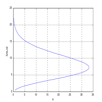
Figure 1: Graph of a dependence entropy vs. area for a unit hyper-spheres

Therefore

$$D={S\over Kln~{}2}\equiv s.$$

On the other hand,the $(D-1)$-dim hyper-area enclosing a $D$- dimensional( bulk) hyper-volume of a $D$-dimensional sphere of a unit Planck radius is :

$$A_{D-1}=D{{\sqrt{\pi}}^{D}\over\Gamma({D+2\over 2})}.$$

which means that $D$ and hence $s$ ( eq.B1) is an implicit function of the hyper-area $A$:

$$s=D(A)$$

Since this function cannot be expressed analytically we restrict ourselves to its graphical representation shown in Fig. 1. It is easily seen that the graph has a region of a linear dependence $s$ vs. $A$ in a rather narrow range of dimensions, namely from $D=2$ to $D=5$.

The slope of the linear region is $1/6.9$ which is less than the Bekenstein upper bound. For the dimensions outside this range the dependence clearly deviates from linearity. If we consider a sphere with a non-unit radius then a respective graph of $s$ vs. $A$ will look similar to Fig.1, with the only difference that for the same $s$ the values of the respective areas $A$ will increase with the radius increase, as in Fig 2.

Let us apply this result to macroscopic black holes.We can consider a macroscopic black-hole as being built from many ”bits” or mini black holes of unit Planck radius. The state of a macroscopic black-hole is evaluated by simply ”counting ” the number of micro-states accessible to the macroscopic system.

Since Bekenstein and Hawking assumed that there exists a linear relation between area and entropy (valid only for a certain range of dimensions, as was shown above) , the entropy could be found by simply adding elementary portions (or bits) of areas. In other words, a linear superposition of the fundamental mini black holes states was possible due to the linearity of the area-entropy relation . A more general way of combining bits of information-entropy is as follows.

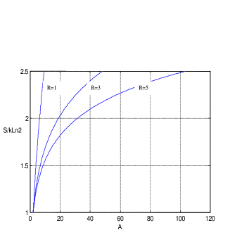
Figure 2: Graph of a dependence entropy vs. area for hyper-spheres of 3 different radii: R=1, 3, and 5

Suppose we wish to calculate the entropy of a cubic object. Since a cube is topologically equivalent to a sphere, we simply deform the cube into a sphere, simultaneously preserving the cube’s area. This leads to an increase of the sphere’s volume as compared to the original cube. As a next step we evaluate the surface area of the sphere suitably normalized to Planck units. If now we divide this area by the area of a unit sphere (in Planck units) then the result would give us the information entropy ( divided by $KLn2$) of the original cube.

However there are two obvious objections to this procedure:

1.Is it possible to pack all unit spheres into the big sphere without leaving any voids ?

2. What if the information-entropy, given by the ratio of areas (in units of $kln~{}2$) is not an integer ?

To answer the first objection we perform an inverse deformation of each unit sphere into a fundamental small cube of the same area, then we deform the large sphere into the original cube of the same area. Now we can pack all the elementary cubes into a large cube without leaving voids.

The second objection is a little bit more tricky. In this case a small region of the cube remains unpacked. To resolve this problem we use properties of fractal geometry: the large cube is to be filled with cubes of fractal dimensions. Since fractals have a property of space filling the cube will be filled without any voids left.

Now we make a plausible assumption that only one bit of information can be ascribed to a minimum attainable scale, the Planck scale $\Lambda.$ This assumption is supported by the holographic origins of chaos in $M$ theory [39]. An onset of chaos is signaled by impossibility to pack the energy levels ( spectra ) into small regions of very high energy ( spectral ) density distributions. The repulsive ( holographic ) feature of these spectral lines is the indication of quantum chaos.

This means that for every two adjacent cubes/cells packed side by side, information will be ”pushed” out to the respective surfaces. As a result their common boundary surface would contain two bits of information per unit area (in Planck units) , which contradicts our initial assumption that one cannot have more than one bit per unit area ( an ” exclusion principle ”). Applying this argument to the overall packing-process we arrive at a situation analogous to the Gauss’s law in electrostatics: the information can reside only on the boundary surface of a cube, and hence on the surface of the original sphere. For the importance of the Cantorian fractal spacetime model for the theory of superconductivity, and its potential high temperature applications, see [40].

In general, the graphs $s=D(A)$ (figs. $1$ and $2$) exhibit a variable slope indicating that information density changes with the area. The slope reaches infinity in two cases: 1) at a maximum attainable area and 2)in the limit of $D\rightarrow\infty$ when the area goes to $0$. The latter signals an onset of a phase transition under which spacetime ”evaporates” leaving behind a fractal Cantor dust. Since the area tends to $0$ the information density blows up.

In the former case ( for simplicity consider a unit sphere) the slope becomes infinite between $D=4$ and $D=5$. This is the metastable renormalization group fixed point of $D$= $4$+$\epsilon$ = $4$ + $\phi^{3}$. Not surprisingly, this is another physical reason why we live in $D=4$. Can we actually reach $D=\infty$ ? In other words, how much energy this process would require? In [11] we have discussed why dimensions, energy, information are indistinguishable at the ultimate scale provided by nature, the Planck scale $\Lambda$. Once Nottale’s scale relativistic corrections to resolutions of physical devices are taken into account, it turns out that to reach $D=\infty$ (which is tantamount to reaching the Planck scale [13]) one needs an infinite amount of energy.

9 Appendix C

Renormalization group flow and a local scaling arrow of time.

Here we would like to point out a connection of our work to the renormalization group techniques of quantum field theory within the context of fractals. The emergence of a microscopic Liouville arrow of time within the context of $D$-branes and the breakdown of Lorentz invariance at very short scales has been analyzed by Ellis et al [18]. In a sense, a picture of an infinite unfolding of a hierarchy of infinite-dimensional worlds represents a visualization of actions of the renormalization group. In simple terms we can recreate this picture as follows. Let us focus our eyes at a small region of a monitor which we will conditionally call a ”point”. Certainly one can even imagine to be ”inside” this point. A physical realization of this immersion would require a lot of energy which will increase with a decrease of the point’s size. As more energy is supplied to get inside the ”point ” (corresponding to a greater zoom) an observer will notice unfolding of additional dimensions. This resembles playing with a toy matryoshka doll. Since energy generates information ( and generated by information) an increase of energy in this process will generate additional information and as a result will reverse a local microscopic scaling arrow of time.

We begin to move into a different hierarchical family of the Cantorian matryoshka-like spacetimes whose local average dimension will be greater than our initial $D=4$. The opening worlds would be the members of the family which belongs to our ”past” with respect to the local scaling renormalization group arrow of time. However to reverse the renormalization group arrow of time of the whole (global) universe is a totally different enterprise because energy involved in achieving such a feat would be enormous, of the order of the total mass-energy of the whole universe.

Kreimer [25] has provided an ample proof that the renormalization and combinatorial techniques of quantum field theory contains a Hopf algebra associated with the Feynamn’s diagrams. A multi fractal, multi-vector , and multi-scaling basis of a new relativity allows one to utilize a rich and diverse mathematical apparatus of quantum groups, noncommutative geometry, Feynman graphs, Hopf algebras, etc. as an algebraic-combinatorial and self-recursive way of coding the infinite unfolding of the transfinite Cantorian multi fractal hierarchical matryoshka doll-like worlds. Interestingly enough, the Euler gamma function ( which is self-recursive and which plays an important role in our derivation)is an essential tool in the renormalization process of quantum field theory.

To make our statement about reversing a scaling arrow of time more precise we invoke Zamolodchikov’s central charge theorem [41] which originally was formulated for flows in conformal field theories in $D=2$ but can be easily generalized to $D=2n$. The theorem states that the central charge $c[g^{i},\mu]$ monotonically decreases along its renormalization group trajectory moving towards the infrared region

$${\partial g^{i}\over\partial ln~{}\mu}~{}{\partial c[g^{i},\mu]\over\partial g^{i}}={\partial c[g^{i},\mu]\over\partial ln~{}\mu}\leq 0.$$

Here $g^{i}$ are the world sheet couplings and $\mu$ is the scale,or the subtraction point.

On the other hand, in string theory and conformal field theory central charges are directly related to dimensions. For example, critical strings are anomaly free in $D=26$ to cancel the $c=-26$ charge associated with the ghosts; critical superstrings are anomaly free in $D=10$, etc. This fact indicates that our assertion about ” reversal” of the scaling renormalization group flow on its way to regions of higher central charges and hence higher dimensions is compatible with Zamolodchikov’s theorem. Moreover, there exists a connection between conformal field theory , the monster group, and sphere packing which could be found in ref. [42]. Roughly speaking , the monster group associated with the Golay error correcting code for a self-recursive system encodes the unfolding process into higher dimensions. And conversely, upon reversal of the scaling arrow of time, the monster group encodes condensation of dimensions from the higher( on the average) initial values to the smaller ( on the average ) values. This could be viewed as coding a monotonic (quasi) crystallization process. Similar ideas about a code underlying spacetime being a q-network of q-processes was expressed by Finkelstein long time ago [43].

References

- [1] M.S. El Naschie : Int. Jour, Theor. Physics 12 (1998) 2935.
- [2] L. Nottale : ” Fractal Spacetime and Microphysics : Towards a Theory of Scale Relativity ” World Scientific, 1993; ” La Relativite dans tous ses Etats ” Hachette Literature, Paris, 1998.
- [3] E.Witten ”Reflections on the Fate of Spacetime”, Physics Today,24, April 1996.
- [4] A. Aurilia, S. Ansoldi , E. Spallucci, J. Chaos, Solitons and Fractals. 10(2-3) (1999) 197 .
- [5] L. Smolin, S. Kaufmann , ” Combinatorial Dynamics in Quantum Gravity ” hep-th/9809161.
- [6] R. Cahill, C. Klinger , ” Self Referential Noise as a Fundamental Aspect of Reality ” gr-qc/9905082.
- [7] T. Nowotny, M. Requardt, J. Chaos, Solitons and Fractals. 10(2-3) (1999) 469.
- [8] C. Castro : ” Hints of a New Relativity Principle from -Brane Quantum Mechanics ” to appear in the J. Chaos, Solitons and Fractals;” The Search for the Origins of Theory : Loop Quantum Mechanics and Bulk/Boundary Duality ” hep-th/9809102 S.Ansoldi, C. Castro, E. Spallucci : ” String Representation of Quantum Loops ” Class. Quant. Gravity 16 (1999) 1833 hep-th/9809182
- [9] C.Castro : ” Is Quantum Spacetime Infinite Dimensional ? ” to appear in J. Chaos, Solitons and Fractals.
- [10] C. Castro : ” The String Uncertainty Relations follow from the New Relativity Theory ” hep-th/0001023 ( to be published in Foundations of Physics)
- [11] C. Castro, Alex Granik : ” On Theory, Quantum Paradoxes and the New Relativity ” physics/ 0002019; ”How a New Scale Relativity Resolves Some Quantum Paradoxes”, J.Chaos, Solitons, and Fractals 11(11) (2000), to be published.
- [12] L. Smolin : Private Communication to CC.
- [13] C. Castro : ” An Elementary Derivation of the Black-Hole Area-Entropy Relation in Any Dimension ” hep-th/0004018 submitted to the Jour. of Information Theory and Entropy.
- [14] M.S. El Naschie : ” von Neumann Geometry and Quantum Spacetime ” , J. Chaos, Solitons and Fractals. 9 (1998) 2023.
- [15] M.S. El Naschie :”Fractal Gravity and Symmetry Breaking in a Hierarchical Cantorian-Spacetime ” J. Chaos, Solitons and Fractals. 8 (11) (1997 ) 1865; ” Nuclear Spacetime Theories, Superstrings, Monster Group and Applications ”, J. Chaos, Solitons and Fractals. 10(2-3) (1999) 567; ” Towards a Geometric Theory for the Unification of all Fundamental Forces based on Cantorian-Fractal Spacetime ” J. Chaos, Solitons and Fractals,bf 11(2000),1459 ;
- [16] G.Ord,J.Chaos,Solitons, and Fractals 10, (2-3) (1999)499
- [17] D. Mugnai, A. Ranfagni and R. Ruggeri, Phys. Rev. Letts. 84 (2000) 4830.
- [18] J. Ellis, N. Mavromatos, D.Nanopolous, J. Chaos, Solitons and Fractals 10 ( 2-3) (1999) 345.
- [19] A. Aurilia, S. Ansoldi , C. Castro and E. Spallucci, In preparation
- [20] W.Pezagglia, ” Dimensionally Democratic Calculus and Principles of Polydimensional Physics ” gr-qc/9912025
- [21] G. Chapline, K. Yagamishi, ” Induced Self Dual Gravity : a algebraic approach ”, Class. Quantum. Gravity 8 (1991) 427.
- [22] H.Peres Rojas, R.Torres, Phys.Letts A 137(1989) 126
- [23] M.S. El Naschie, ”On the Electroweak Mixing Angle in ”,J. Chaos, Solitons and Fractals 11 (2000) 1803 3
- [24] M.S. El Naschie, O. Rossler , G. Ord , ”Introduction to Chaos, Information and Diffusion in Quantum Mechanics ” J. Chaos, Solitons and Fractals 7 (5) (1996) May issue.
- [25] D.Kreimer, Shuffling Quantum Field Theory, hep-th/9912290
- [26] D. Chakalov , Private Communication.
- [27] P.De Bernardis et al ”A flat Universe from high-resolution maps of the cosmic microwave background radiation”, Nature 404 (2000) 955;
- [28] E. Lange, P.Ade, J. Bock et al : ” First Estimations of cosmological Parameters from BOOMERANG ” astro-ph/0005004.
- [29] H. Kitada, ” A Possible Solution to the Nonexistence of Time” gr-qc/9910081.
- [30] J. Vigier, C. Petroni, ” Markov Processes at the velocity of Light, The Klein-Gordon statistics ”,Int. Jour. Theor. Physics 18 (11) (1979) 807.
- [31] B. Sidharth , ” A Brief Note on Fluctuations and Interactions ” to appear in the J. Chaos, Solitons and Fractals.
- [32] C.Castro,”Conformally Invariant models on anti de Sitter Spaces, Chern-Simons -branes and Geometry” hep-th/9906176
- [33] M.Vasiliev, ”Higher Spin Gauge Theries in Four,Three, and Two Dimensions” hep-th/9611024
- [34] C.Castro,Jour. of Geometry and Physics 33 (2000) 173
- [35] M. Pitkannen ”-Adic TGD Mathematical Ideas ” hep-th/9506097; Khrennikov ” -Adic numbers in QM, … ” quant-ph/9506097; Vladimorov, I. Volovich, E. Zelenov : ” =Adic numbers in Mathematical physics ”. World Scientific 1994; Brekke and P. Freund, Phys. Reports 231 (1993) 1-66; Altaisky, B. Sidharth, J. Chaos, Solitons and Fractals 0 ( 2-3) (1999) 167; Ghoshal, A. Sen, ”Tachyon Condensation and Brane Descent Relations in p-adic String Theory ” hep-th/0003278.
- [36] D. Koruga, ” Information Physics : In Search of the Scientific Basis of Consciousness ” Edited by S. Hameroof et al M.I.T press 1995.
- [37] R.Feynman and A.Hibbs, ”Quantum Mechanics and Path Integrals”,McGraw-Hill Co,1965;M.Abbott and M.Wise, Am.J.Phys 49 (1)(1981)
- [38] L.Abbot, M.Wise,, Am. J.Phys., 49 (1) (1981)
- [39] I. Aref’eva, P. Medvedev, O. Rytchkov and I. Volovich , J.Chaos, Solitons and Fractals. 10(2-3) (1999) 213.
- [40] M. Agop, P. Ioannu, P. Coman,B. Ciobanu and P. Nica, Cantorian-Fractal spacetime and Generalized Superconductivity ”, submitted to J.Chaos,Solitons and Fractals
- [41] A.Zamolodchikov, JETP Lett. 43(1986), 730; Sov.J.Nucl.Phys. 46(1987),1090
- [42] T.Gannon, ”Monstrous moonshine and the classification of CFT” QA/9906167
- [43] D. Finkelstein, ” Spacetime Code ” Phys. Review D 5 (1972) 320;Phys. Review D 5 (1972) 2922; Phys. Review D 9 (1974) 2219