The tachyon potential in Witten’s superstring field theory

Abstract:

We study the tachyon potential in the NS sector of Witten’s cubic superstring field theory. In this theory, the pure tachyon contribution to the potential has no minimum. We find that this remains the case when higher modes up to level two are included.

1 Introduction

It has been conjectured by Sen that at the stationary point of the tachyon potential for the D-brane-anti-D-brane pair or for the non-BPS D-brane of superstring theories, the negative energy density precisely cancels the brane tensions [1].

For the D-brane of bosonic string theory, this conjecture has been verified [2] starting from Witten’s open string field theory [3] and in the supersymmetric case starting from Berkovits’ superstring field theory [4]–[8].

In this paper we study the tachyon potential in the NS sector of Witten’s superstring field theory [9]. Soon after this theory was proposed, it became clear that it suffered some problems [10]. Infinities were found to arise in the calculation of tree-level scattering amplitudes. These find their origin in picture-changing operators inserted at the same point. Similar problems arise in the proof of gauge invariance of the action. Modifications of Witten’s action have been proposed in order to solve these issues [11], but these seem to suffer from other difficulties [4]. In the light of these problems, the present calculation should be seen as a further study of Witten’s string field theory proposal rather than as a test of Sen’s conjecture, which has been extensively verified on a quantitative level.

We use the level truncation method of Kostelecky and Samuel [12] retaining fields up to level 2 and terms up to level 4 in the action. We find that the tachyon potential in this theory does not have the behaviour conjectured by Sen, in fact it doesn’t even have a minimum. This is already the case for the pure tachyon contribution (in contrast to the pure tachyon contribution is Berkovits’ theory [5]), and this behaviour is found to persist when higher modes are included.

2 Witten’s superstring field theory in CFT language

In this section we review Wittens string field theory for open superstrings [3, 9] formulated in the conformal field theory (CFT) approach [13]. We restrict our attention to fields in the NS sector of the theory.

In the CFT approach, a general NS-sector string field $A$ is represented by a CFT vertex operator of ghost number $1$ and picture number $-1$. The superghosts are bosonized as $\beta=\partial\xi e^{-\phi}$ and $\gamma=\eta e^{\phi}$ [14] and the string field $A$ is restricted to live in the “small” Hilbert space of the bosonized system, i.e. it does not include the $\xi$ zero mode. The string field should also satisfy a suitable reality condition in order for the action to take real values.

Witten proposed a Chern-Simons type action

$$S=-\left\langle\left\langle\!\right.\right.A\ Q_{B}A\left.\left.\!\right\rangle\right\rangle-\frac{2}{3}\left\langle\left\langle\!\right.\right.A^{3}\left.\left.\!\right\rangle\right\rangle,$$ (1)

where $Q_{B}$ is the BRST charge

$$Q_{B}=\oint dzj_{B}(z)=\oint dz\Bigl{\{}c\bigl{(}T_{m}+T_{\xi\eta}+T_{\phi})+c\partial cb+\eta\,e^{\phi}\,G_{m}-\eta\partial\eta e^{2\phi}b\Bigr{\}}\,,$$

and the double brackets should be interpreted as a CFT correlator with extra picture-changing insertions:

$$\left\langle\left\langle\!\right.\right.\Phi_{1}\Phi_{2}\cdots\Phi_{n-1}\Phi_{n}\left.\left.\!\right\rangle\right\rangle=$$ (2)

$$=\Big{\langle}Y(0)f_{1}^{n}\circ\Phi_{1}(0)X(0)f_{2}^{n}\circ\Phi_{2}(0)X(0)\cdots X(0)f_{n-1}^{n}\circ\Phi_{n-1}(0)X(0)f_{n}^{n}\circ\Phi_{n}(0)\Big{\rangle}\,.$$

The symbols $f_{i}^{n}$ denote conformal transformations mapping the unit circle to wedge-formed pieces of the complex-plane:

$$f^{n}_{k}(z)=e^{2\pi i(k-1)/n}\left(\frac{1+iz}{1-iz}\right)^{2/n}\quad\hbox{for}\ n\geq 1\,.$$

The operators $X$ and $Y$ are the picture-changing and inverse picture-changing operators, respectively:

$$X = -\partial\xi c+e^{\phi}G_{m}-\partial\eta\ be^{2\phi}-\partial\left(\eta be^{2\phi}\right),$$

$$Y = -\partial\xi ce^{-2\phi}\,.$$

They are each others inverse in the following sense:

$$\lim_{\epsilon\rightarrow 0}Y(z+\epsilon)X(z)=1\,.$$

The action is formally invariant under the gauge transformations

$$\delta A=Q_{B}\epsilon+A\epsilon-\epsilon A\,,$$

where $\epsilon$ is a NS string field of ghost number 0 in the $-1$ picture. The proof of the gauge invariance relies on the following properties of the correlator (2)

$$\left\langle\left\langle\!\right.\right.Q_{B}(\Phi_{1}\cdots\Phi_{n})\left.\left.\!\right\rangle\right\rangle = 0\,,$$

$$\left\langle\left\langle\!\right.\right.\cdots Q_{B}^{2}(\Phi_{1}\cdots\Phi_{n})\cdots\left.\left.\!\right\rangle\right\rangle = 0\,,$$

$$\left\langle\left\langle\!\right.\right.\cdots Q_{B}(A\Phi)\cdots\left.\left.\!\right\rangle\right\rangle = \left\langle\left\langle\!\right.\right.\cdots(Q_{B}A\ \Phi-A\ Q_{B}\Phi)\cdots\left.\left.\!\right\rangle\right\rangle,$$

$$\left\langle\left\langle\!\right.\right.\cdots Q_{B}(\epsilon\Phi)\cdots\left.\left.\!\right\rangle\right\rangle = \left\langle\left\langle\!\right.\right.\cdots(Q_{B}\epsilon\ \Phi+\epsilon\ Q_{B}\Phi)\cdots\left.\left.\!\right\rangle\right\rangle,$$

$$\left\langle\left\langle\!\right.\right.\Phi_{1}\cdots\Phi_{n-1}\Phi_{n}\left.\left.\!\right\rangle\right\rangle = \left\langle\left\langle\!\right.\right.\Phi_{n}\Phi_{1}\cdots\Phi_{n-1}\left.\left.\!\right\rangle\right\rangle.$$ (3)

$A$ and $\epsilon$ represent the string field and the gauge parameter respectively and the $\Phi_{i}$ represent arbitrary operators in the GSO(+) sector.

These properties suffice to prove the gauge invariance of the action. Such a “proof” should be taken with a grain of salt however since it involves manipulating correlators with four string fields. From the definition (2), one sees that such correlators contain 2 insertions of the picture-changing operator at the origin and are hence divergent. These and other problems of the action (1) were discussed in [10].

3 Witten’s string field theory on a non-BPS D-brane

In order to describe NS excitations on a non-BPS D-brane, one should extend the theory to include also states with odd world-sheet fermion number. This can be accomplished by tensoring the fields entering in the action and gauge transformation with suitable internal Chan-Paton (CP) factors as in [5, 6]. The fields with CP factors attached are denoted with hats. We take the following assignments for the internal CP factors:

$${\widehat{A}} = A_{+}\otimes I+A_{-}\otimes\sigma_{1}\,,$$

$$\widehat{\epsilon} = \epsilon_{+}\otimes\sigma_{3}+\epsilon_{-}\otimes i\sigma_{2}\,,$$

$${\widehat{Q}_{B}} = Q_{B}\otimes\sigma_{3}\,,$$

$$\widehat{Y} = Y\otimes I\,,$$

$$\widehat{X} = X\otimes\sigma_{3}\,,$$ (4)

where $I$ is the $2\times 2$ unit matrix and $\sigma_{i}$ are the Pauli matrices. The action takes the form

$$S=-\left\langle\left\langle\!\right.\right.{\widehat{A}}\ {\widehat{Q}_{B}}{\widehat{A}}\left.\left.\!\right\rangle\right\rangle-\frac{2}{3}\left\langle\left\langle\!\right.\right.{\widehat{A}}^{3}\left.\left.\!\right\rangle\right\rangle,$$

where the double brackets should now be interpreted as

$$\left\langle\left\langle\!\right.\right.{\widehat{\Phi}}_{1}{\widehat{\Phi}}_{2}\cdots{\widehat{\Phi}}_{n-1}{\widehat{\Phi}}_{n}\left.\left.\!\right\rangle\right\rangle = \frac{1}{2}\mathop{\rm Tr}\nolimits\Big{\langle}\widehat{Y}(0)f_{1}^{n}\circ{\widehat{\Phi}}_{1}(0)\widehat{X}(0)f_{2}^{n}\circ{\widehat{\Phi}}_{2}(0)\times$$

$$\hphantom{\frac{1}{2}\mathop{\rm Tr}\nolimits\Big{\langle}}\!\times\,\widehat{X}(0)\cdots\widehat{X}(0)f_{n-1}^{n}\circ{\widehat{\Phi}}_{n-1}(0)\widehat{X}(0)f_{n}^{n}\circ{\widehat{\Phi}}_{n}(0)\Big{\rangle}\,.$$

The trace runs over the internal CP indices. The gauge transformations are

$$\delta{\widehat{A}}={\widehat{Q}_{B}}\widehat{\epsilon}+{\widehat{A}}\widehat{\epsilon}-\widehat{\epsilon}{\widehat{A}}\,.$$ (5)

The CP factor assignments (4) were chosen such that gauge transformations preserve the CP structure of the string field:

$$\delta{\widehat{A}}=\delta A_{+}\otimes I+\delta A_{-}\otimes\sigma_{1}$$

and such that the algebraic structure (3) is preserved:

$$\left\langle\left\langle\!\right.\right.{\widehat{Q}_{B}}({\widehat{\Phi}}_{1}\cdots{\widehat{\Phi}}_{n})\left.\left.\!\right\rangle\right\rangle = 0\,,$$

$$\left\langle\left\langle\!\right.\right.\cdots{\widehat{Q}_{B}}^{2}({\widehat{\Phi}}_{1}\cdots{\widehat{\Phi}}_{n})\cdots\left.\left.\!\right\rangle\right\rangle = 0\,,$$

$$\left\langle\left\langle\!\right.\right.\cdots{\widehat{Q}_{B}}({\widehat{A}}{\widehat{\Phi}})\cdots\left.\left.\!\right\rangle\right\rangle = \left\langle\left\langle\!\right.\right.\cdots({\widehat{Q}_{B}}{\widehat{A}}\ {\widehat{\Phi}}-{\widehat{A}}\ {\widehat{Q}_{B}}{\widehat{\Phi}})\cdots\left.\left.\!\right\rangle\right\rangle,$$

$$\left\langle\left\langle\!\right.\right.\cdots{\widehat{Q}_{B}}(\widehat{\epsilon}{\widehat{\Phi}})\cdots\left.\left.\!\right\rangle\right\rangle = \left\langle\left\langle\!\right.\right.\cdots({\widehat{Q}_{B}}\widehat{\epsilon}\ {\widehat{\Phi}}+\widehat{\epsilon}\ {\widehat{Q}_{B}}{\widehat{\Phi}})\cdots\left.\left.\!\right\rangle\right\rangle,$$

$$\left\langle\left\langle\!\right.\right.{\widehat{\Phi}}_{1}\cdots{\widehat{\Phi}}_{n-1}{\widehat{\Phi}}_{n}\left.\left.\!\right\rangle\right\rangle = \left\langle\left\langle\!\right.\right.{\widehat{\Phi}}_{n}{\widehat{\Phi}}_{1}\cdots{\widehat{\Phi}}_{n-1}\left.\left.\!\right\rangle\right\rangle.$$

With these properties (proven in appendix B), the (formal) proof of gauge invariance goes through as in the GSO(+) sector.

4 The fields up to level 2

In the calculation of the tachyon potential, we can restrict the string field to lie in a subspace ${\cal H}_{1}$ formed by acting only with modes of the stress-energy tensor, the supercurrent and the ghost fields $b,\ c,\ \eta,\ \xi,\phi$ since the other excitations can be consistently put to zero [1]. We fix the gauge freedom (5) by imposing the Feynman-Siegel gauge $b_{0}{\widehat{A}}=0$ on fields with non-zero conformal weight. Taking all this together we get the following list of contributing fields up to level 2. The level of a field is just the conformal weight shifted by 1/2, in this way the tachyon is a level 0 field. We use the notation $|q\rangle$ for the state corresponding with the operator $e^{q\phi}$.

Table 1: The level $0$,$1$ and $2$ fields should be tensored with $\sigma_{1}$ and the level $1/2$ and $3/2$ fields with $I$. We list the conformal transformations of the fields in appendix A.

Level	GSO	state	vertex operator
0	$-$	$c_{1}|-1\rangle$	$T=ce^{-\phi}$
1/2	$+$	$\xi_{-1}c_{1}c_{0}|-2\rangle$	$R=\partial\xi c\partial c\ e^{-2\phi}$
1	$-$	$c_{1}\phi_{-1}|-1\rangle$	$S=c\partial\phi\ e^{-\phi}$
3/2	$+$	$2c_{1}c_{-1}\xi_{-1}|-2\rangle$	$A=c\partial^{2}c\partial\xi\ e^{-2\phi}$
		$\eta_{-1}|0\rangle$	$E=\eta$
		$c_{1}G^{m}_{-3/2}|-1\rangle$	$F=cG^{m}\ e^{-\phi}$
2	$-$	$c_{1}\left[(\phi_{-1})^{2}-\phi_{-2}\right]|-1\rangle$	$K=c\ \partial^{2}\left(e^{-\phi}\right)$
		$c_{1}\phi_{-2}|-1\rangle$	$L=c\ \partial^{2}\phi\ e^{-\phi}$
		$c_{1}L^{m}_{-2}|-1\rangle$	$M=cT^{m}\ e^{-\phi}$
		$2c_{-1}|-1\rangle$	$N=\partial^{2}c\ e^{-\phi}$
		$\xi_{-1}\eta_{-1}c_{1}|-1\rangle$	$P=\partial\xi\eta c\ e^{-\phi}$

5 The tachyon potential

We have calculated the tachyon potential involving fields up to level 2, including only the terms up to level 4 (the level of a term in the potential is defined to be the sum of the levels of the fields entering into it). We have performed the actual computation in the following way: the conformal tranformations of the fields were calculated by hand and the computation of all the correlation functions between these transformed fields was done with the help of Mathematica. We have written a program to compute the necessary CFT correlation functions.

We denote (subscripts refer to the level)

$$\widehat{\Phi} = t\widehat{T}+ir\widehat{R}+is\widehat{S}+a\widehat{A}+e\widehat{E}+f\widehat{F}+k\widehat{K}+l\widehat{L}+m\widehat{M}+n\widehat{N}+p\widehat{P}\,,$$

$$S(\widehat{\Phi}) = S_{0}+S_{1/2}+S_{1}+S_{3/2}+S_{2}+S_{5/2}+S_{3}+S_{7/2}+S_{4}\,.$$

The factors of $i$ are included because of the reality condition on the string field. We have obtained the following result:

$$S_{0} = \frac{t^{2}}{2}\,,\qquad S_{1/2}=\frac{9}{2}\ r\ t^{2}\,,\qquad S_{1}=-2\,r^{2}\,,$$

$$S_{3/2} = 8\,r\,s\,t-10\,a\,t^{2}+2\,e\,t^{2}-20\,f\,t^{2}\,,$$

$$S_{2} = -\frac{1}{2}s^{2}\,,$$

$$S_{5/2} = \frac{16}{3\,\sqrt{3}}\,e\,{r^{2}}+\frac{10}{3}\,r\,s^{2}-\frac{23}{3}\,k\,r\,t-\frac{25}{2}\,m\,r\,t+2\,n\,r\,t-p\,r\ t-$$

$$-\,\frac{64}{3}\,a\,s\,t-\frac{80}{3}\,f\,s\,t\,,$$

$$S_{3} = -4\,a\,e-10\,f^{2}\,,$$

$$S_{7/2} = -\frac{64}{3\,\sqrt{3}}\,a\,e\,r+\frac{32}{9\ \sqrt{3}}\,e^{2}\,r-\frac{320}{9\,\sqrt{3}}\,e\,f\,r+\frac{320}{9\,\sqrt{3}}\,f^{2}\,r-$$

$$-\,8\,k\,r\,s+\frac{160}{27}\,l\,r\,s-\frac{100}{9}\,m\,r\,s+\frac{80}{9}\,n\,r\,s+\frac{152}{27}\,p\,r\,s+$$

$$+\,\frac{460}{27}\,a\,k\,t-\frac{28}{27}\,e\,k\,t+\frac{280}{27}\,f\,k\,t+\frac{128}{27}\,a\,l\,t+\frac{64}{27}\ e\,l\,t+\frac{250}{9}\,a\,m\,t-$$

$$-\,\frac{50}{9}\,e\,m\,t+\frac{220}{3}\,f\,m\,t-\frac{104}{9}\,a\,n\,t+\frac{40}{9}\,e\,n\,t-\frac{880}{27}\ f\,n\,t+$$

$$+\,\frac{20}{9}\,a\,p\,t-\frac{4}{9}\,e\,p\,t-\frac{200}{27}\,f\,p\,t\,,$$

$$S_{4} = -6\,{k^{2}}+6\,k\,l-3\,{l^{2}}-\frac{45}{4}\,{m^{2}}+6\,{n^{2}}+\frac{3}{2}\,{p^{2}}\,.$$

Taking a look at the potential, we notice immediately that the $Z_{2}$ twist symmetry of Berkovits’ theory is absent in Witten’s theory. Indeed, if this symmetry were present the fields $r$ and $t$ would carry twist charge $-1$ and $+1$, respectively and the $rt^{2}$ term would be constrained to vanish. The origin of this difference between the two theories can be traced to the different structure of their lagrangians: in Berkovits’ action, all operators are inserted on the boundary of the disc, while in Witten’s action there is always an insertion of the picture-changing operator in the origin. The proof of twist invariance of the former theory [6] breaks down for Witten’s theory since it makes use of transformations that do not leave the origin invariant and hence move the picture-changing operator away from the origin.

At level 1 and 2 the fields $r$ and $s$ can be integrated out exactly to give the following effective potentials:

$$V_{0}(t) = -\frac{{t^{2}}}{2}\,,\qquad V_{1}(t)=-\frac{{t^{2}}}{2}-\frac{81\,{t^{4}}}{32}\,,$$

$$V_{2}(t) = -\frac{{t^{2}}}{2}+\frac{81\,{t^{4}}}{2\,{{(4-64\,{t^{2}})}^{2}}}-\frac{648\,{t^{6}}}{{{(4-64\,{t^{2}})}^{2}}}-\frac{81\,{t^{4}}}{4\,(4-64\ {t^{2}})}\,.$$

We see that the inclusion of these higher modes does not alter the fact that the potential has no minimum, in fact, its slope becomes even steeper and a singularity is encountered at level 2, see figure 1. The singularity in the tachyon potential encountered here might be contrasted with the singularities in the tachyon potential of open bosonic string theory found in [2]. In the case at hand, the potential diverges at the singular point. Moreover, it doesn’t have the interpretation as a point where different branches of the effective potential come together since, at level 2, the equations for the fields that are integrated out are linear.

Integrating out the fields numerically for the higher levels, one finds that the more fields are included, the steeper the slope of the potential becomes. This behaviour was anticipated in the conclusions of [6].

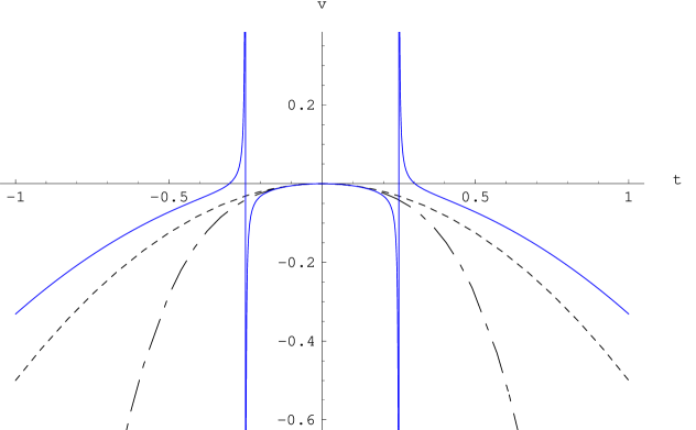
Figure 1: The tachyon potential $V(t)$ at level 0 (dotted line), level 1 (dashed line) and level 2 (full line).

6 Conclusions

In this letter we calculated the tachyon potential in the NS sector of Witten’s superstring field theory. We used a level truncation method and kept terms up to level four in the potential. We found that the potential does not exhibit the expected minimum, and that the situation seems to become worse the more levels are included. This result, in addition to other problems encountered within this formulation, seems to point towards Berkovits’ string field theory proposal as a more viable candidate for the description of off-shell superstring interactions.

Appendix A The conformal transformations of the fields

We now list the conformal transformations of the fields used in the calculation of the tachyon potential. To shorten the notation we denote $w=f(z)$.

$$f\circ T(z) = (f^{\prime}(z))^{-1/2}T(w)\,,$$

$$f\circ R(z) = R(w)\,,$$

$$f\circ S(z) = (f^{\prime}(z))^{1/2}S(w)-\frac{1}{2}\frac{f^{\prime\prime}(z)}{f^{\prime}(z)}(f^{\prime}(z))^{-1/2}ce^{-\phi}(w)\,,$$

$$f\circ A(z) = f^{\prime}(z)A(w)-\frac{f^{\prime\prime}(z)}{f^{\prime}(z)}c\partial c\,\partial\xi\,e^{-2\phi}(w)\,,$$

$$f\circ E(z) = f^{\prime}(z)E(w)\,,$$

$$f\circ F(z) = f^{\prime}(z)F(w)\,,$$

$$f\circ K(z) = (f^{\prime}(z))^{3/2}K(w)+2\frac{f^{\prime\prime}(z)}{f^{\prime}(z)}(f^{\prime}(z))^{1/2}c\partial\left(e^{-\phi}\right)(w)+$$

$$+\left[\frac{1}{2}\frac{f^{\prime\prime\prime}}{f^{\prime}}-\frac{1}{4}\left(\frac{f^{\prime\prime}}{f^{\prime}}\right)^{2}\right](f^{\prime}(z))^{-1/2}ce^{-\phi}(w)\,,$$

$$f\circ L(z) = (f^{\prime}(z))^{3/2}L(w)+\frac{f^{\prime\prime}(z)}{f^{\prime}(z)}(f^{\prime}(z))^{1/2}c\partial\phi\,e^{-\phi}(w)+$$

$$+\left[\frac{3}{4}\left(\frac{f^{\prime\prime}}{f^{\prime}}\right)^{2}-\frac{2}{3}\frac{f^{\prime\prime\prime}}{f^{\prime}}\right](f^{\prime}(z))^{-1/2}ce^{-\phi}(w)\,,$$

$$f\circ M(z) = (f^{\prime}(z))^{3/2}M(w)+\frac{15}{12}\left[\frac{f^{\prime\prime\prime}}{f^{\prime}}-\frac{3}{2}\left(\frac{f^{\prime\prime}}{f^{\prime}}\right)^{2}\right](f^{\prime}(z))^{-1/2}ce^{-\phi}(w)\,,$$

$$f\circ N(z) = (f^{\prime}(z))^{3/2}N(w)-\frac{f^{\prime\prime}(z)}{f^{\prime}(z)}(f^{\prime}(z))^{1/2}\partial c\,e^{-\phi}(w)+$$

$$+\left[2\left(\frac{f^{\prime\prime}}{f^{\prime}}\right)^{2}-\frac{f^{\prime\prime\prime}}{f^{\prime}}\right](f^{\prime}(z))^{-1/2}c\,e^{-\phi}(w)\,,$$

$$f\circ P(z) = (f^{\prime}(z))^{3/2}P(w)+$$

$$+\left[\frac{1}{4}\left(\frac{f^{\prime\prime}}{f^{\prime}}\right)^{2}-\frac{1}{6}\frac{f^{\prime\prime\prime}}{f^{\prime}}\right](f^{\prime}(z))^{-1/2}ce^{-\phi}(w)\,.$$

Appendix B Cyclicity property of string amplitudes

The proof of the cyclicity is based on appendix A of [6]. First we give some preliminary remarks.

It is easy to see that all the fields in the GSO($+$) sector are tensored with either $I$ or $\sigma_{3}$, and all the fields in the GSO($-$) sector with either $\sigma_{1}$ or $i\sigma_{2}$. The fields in the GSO($+$) sector have integer conformal weight, and the fields in GSO($-$) sector have half-integer conformal weight. We compute

$$\left\langle\left\langle\!\right.\right.{\widehat{\Phi}}_{1}\cdots{\widehat{\Phi}}_{n}\left.\left.\!\right\rangle\right\rangle = \mathop{\rm Tr}\nolimits\left\langle\widehat{Y}f_{1}^{n}\circ{\widehat{\Phi}}_{1}\widehat{X}\cdots\widehat{X}f_{n-1}^{n}\circ{\widehat{\Phi}}_{n-1}\widehat{X}f_{n}^{n}\circ{\widehat{\Phi}}_{n}\right\rangle$$

$$= \mathop{\rm Tr}\nolimits\left\langle\widehat{Y}f_{2}^{n}\circ{\widehat{\Phi}}_{1}\widehat{X}\cdots\widehat{X}f_{n}^{n}\circ{\widehat{\Phi}}_{n-1}\widehat{X}\,R\circ f_{1}^{n}\circ{\widehat{\Phi}}_{n}\right\rangle,$$

where $R$ is the rotation over an angle of $2\pi$. Next we use $R\circ f_{1}^{n}\circ{\widehat{\Phi}}_{n}=\pm f_{1}^{n}\circ{\widehat{\Phi}}_{n}$, with a plus sign if the field has integer weight, and a minus sign if the field has half-integer weight. We also use the cyclicity of the trace to move the field ${\widehat{\Phi}}_{n}$ in front. Although we are manipulating grassmann objects, we do not get an additional minus sign, due to the fact that the total amplitude is grassmann odd.

$$\left\langle\left\langle\!\right.\right.{\widehat{\Phi}}_{1}\cdots{\widehat{\Phi}}_{n}\left.\left.\!\right\rangle\right\rangle = \pm\mathop{\rm Tr}\nolimits\left\langle\widehat{Y}f_{1}^{n}\circ{\widehat{\Phi}}_{n}f_{2}^{n}\circ{\widehat{\Phi}}_{1}\widehat{X}\cdots\widehat{X}f_{n}^{n}\circ{\widehat{\Phi}}_{n-1}\widehat{X}\right\rangle$$ (6)

$$= \pm\mathop{\rm Tr}\nolimits\left\langle\widehat{Y}\widehat{X}\circ f_{1}^{n}\circ{\widehat{\Phi}}_{n}f_{2}^{n}\circ{\widehat{\Phi}}_{1}\widehat{X}\cdots\widehat{X}f_{n}^{n}\circ{\widehat{\Phi}}_{n-1}\right\rangle$$

$$= \mathop{\rm Tr}\nolimits\left\langle\widehat{Y}f_{1}^{n}\circ{\widehat{\Phi}}_{n}\widehat{X}f_{2}^{n}\circ{\widehat{\Phi}}_{1}\widehat{X}\cdots\widehat{X}f_{n}^{n}\circ{\widehat{\Phi}}_{n-1}\right\rangle$$

$$= \left\langle\left\langle\!\right.\right.{\widehat{\Phi}}_{n}{\widehat{\Phi}}_{1}\cdots{\widehat{\Phi}}_{n-1}\left.\left.\!\right\rangle\right\rangle.$$

In the next to last line the picture changing operator commutes with the GSO($+$) fields and anticommutes with the GSO($-$) fields, cancelling the minus sign in front of the amplitude.