Dyons with axial symmetry

Abstract

We construct axially symmetric dyons in SU(2) Yang-Mills-Higgs theory. In the Prasad-Sommerfield limit, they are obtained via scaling relations from axially symmetric multimonopole solutions. For finite Higgs self-coupling they are constructed numerically.

1 Introduction

SU(2) Yang-Mills-Higgs (YMH) theory possesses magnetic monopole [1, 2, 3], multimonopole [4, 5, 6] and monopole-antimonopole solutions [7, 8, 9]. The magnetic charge $m$ of these solutions is proportional to their topological charge $n$. In the Prasad-Sommerfield limit of vanishing Higgs self-coupling, the monopole solution and axially symmetric multimonopole solutions are known analytically [2, 5], whereas multimonopole solutions without rotational symmetry [10] and monopole-antimonopole solutions [8, 9] are only known numerically.

SU(2) Yang-Mills-Higgs (YMH) theory also possesses solutions carrying both magnetic and electric charge [11, 2]. In the Prasad-Sommerfield limit, such dyon solutions with unit topological charge exist for arbitrarily large values of the electric charge [2], whereas for finite Higgs self-coupling an upper bound for the electric charge of these dyon solutions arises [12].

Here we construct axially symmetric dyon solutions carrying topological charge $n>1$. In section 2 we present the YMH Lagrangian, the equations of motion and the electromagnetic charges. In section 3 we consider the Prasad-Sommerfield limit, and show how dyon solutions are obtained from multimonopole solutions. We present the axially symmetric ansatz and the boundary conditions employed in the numerical construction of the dyonic multimonopole solutions in section 4, and discuss these solutions in section 5, in particular for finite Higgs self-coupling.

2 SU(2) YMH Theory

We consider the SU(2) YMH Lagrangian

$$L=-\frac{1}{4}F_{\mu\nu}^{a}F^{\mu\nu,a}-\frac{1}{2}D_{\mu}\Phi^{a}D^{\mu}\Phi^{a}-\frac{\lambda}{4}(\Phi^{a}\Phi^{a}-\eta^{2})^{2}\ ,$$ (1)

with

$$F^{a}_{\mu\nu}=\partial_{\mu}A^{a}_{\nu}-\partial_{\nu}A^{a}_{\mu}+g\varepsilon^{abc}A^{b}_{\mu}A^{c}_{\nu}\ ,$$ (2)

$$D_{\mu}\Phi^{a}=\partial_{\mu}\Phi^{a}+g\varepsilon^{abc}A_{\mu}^{b}\Phi^{c}\ ,$$ (3)

gauge coupling constant $g$, Higgs self-coupling constant $\lambda$, Higgs vacuum expectation value $\eta$, and equations of motion

$$D_{\mu}F^{\mu\nu,a} = -g\varepsilon^{abc}(D^{\nu}\Phi^{b})\Phi^{c}\ ,$$

$$D_{\mu}D^{\mu}\Phi^{a} = -\lambda\left(\Phi^{b}\Phi^{b}-\eta^{2}\right)\Phi^{a}\ .$$ (4)

We are looking for static finite energy solutions of eqs. (4), carrying both magnetic and electric charge. The magnetic field $B_{i}$ and the electric field $E_{i}$ are defined via the electromagnetic ‘t Hooft field strength tensor [1]

$${\cal F}_{\mu\nu}=\hat{\Phi}^{a}F_{\mu\nu}^{a}-\frac{1}{g}\varepsilon_{abc}\hat{\Phi}^{a}D_{\mu}\hat{\Phi}^{b}D_{\nu}\hat{\Phi}^{c}\ ,$$ (5)

where in particular

$$E_{i}={\cal F}_{i0}=\partial_{i}(\hat{\Phi}^{a}A_{0}^{a})\ .$$ (6)

For the dyon solutions they yield the magnetic charge $m$ [13],

$$m=\frac{1}{4\pi}\int{\partial_{i}B_{i}d^{3}r}=\frac{n}{g}\ ,$$ (7)

where $n$ is the topological charge of the solutions, and the electric charge $q$

$$q=\int{\partial_{i}E_{i}d^{3}r}\ =\int_{S_{\infty}^{2}}\partial_{i}(\hat{\Phi}^{a}A_{0}^{a})dS_{i}$$ (8)

where $S^{2}_{\infty}$ denotes the 2-dimensional sphere at infinity.

The energy density of the dyon solutions is given by the $tt$-component of the energy momentum tensor. Integration over all space yields their energy

$$E=\int{\left\{\frac{1}{4}F_{ij}^{a}F_{ij}^{a}+\frac{1}{2}F_{i0}^{a}F_{i0}^{a}+\frac{1}{2}D_{i}\Phi^{a}D_{i}\Phi^{a}+\frac{1}{2}D_{0}\Phi^{a}D_{0}\Phi^{a}+\frac{\lambda}{4}(\Phi^{a}\Phi^{a}-\eta^{2})^{2}\right\}d^{3}r}\ .$$ (9)

3 Prasad-Sommerfield limit $\lambda=0$

Let us first consider the Prasad-Sommerfield limit $\lambda=0$. In this limit axially symmetric multimonopole solutions are known analytically [5] and numerically [6].

We now show, that in the static limit dyon solutions are obtained directly from monopole solutions. Assuming that the time component of the gauge field is parallel to the Higgs field in isospace [14],

$$A_{0}^{a}=\alpha\Phi^{a}\ ,$$ (10)

where $\alpha$ is a constant, leads to $D_{0}\Phi^{a}=0$ and $F_{i0}^{a}=\alpha(\partial_{i}\Phi^{a}+g\varepsilon_{abc}A_{i}^{b}\Phi^{c})=\alpha D_{i}\Phi^{a}$. Consequently, the field equations (4) reduce to

$$D_{i}F^{ij,a} = -g\varepsilon_{abc}(1-\alpha^{2})D^{j}\Phi^{b}\Phi^{c}\ ,$$

$$D_{i}D^{i}\Phi^{a} = 0\ ,$$ (11)

and the field equation for the time component of the gauge field coincides with the field equation for the Higgs field. Substituting $\tilde{\Phi}^{a}=\sqrt{1-\alpha^{2}}\Phi^{a}$ into eqs. (11) leads to the monopole equations.

Thus, to any static solution $(A_{i}^{a},\tilde{\Phi}^{a})$ of the monopole equations in the Prasad-Sommerfield limit with $||\tilde{\Phi}^{a}||\stackrel{{\scriptstyle r\rightarrow\infty}}{{\longrightarrow}}\tilde{\eta}$ there corresponds a family of dyon solutions

$$\left(A_{i}^{a}\ ,\ \ A_{0}^{a}=Q\tilde{\Phi}^{a}\ ,\ \ \Phi^{a}=\sqrt{1+Q^{2}}\tilde{\Phi}^{a}\right)\ ,$$ (12)

with ${\displaystyle||\Phi^{a}||\stackrel{{\scriptstyle r\rightarrow\infty}}{{\longrightarrow}}\tilde{\eta}\sqrt{1+Q^{2}}}$, where we have introduced

$$Q=\alpha/\sqrt{1-\alpha^{2}}\ .$$ (13)

Let us now turn to the energy of the dyon solutions. If $(A_{i}^{a},\tilde{\Phi}^{a})$ is a solution of the monopole equations, it extremizes the energy functional

$$E_{{\rm MP}}=\int{\left\{\frac{1}{4}F_{ij}^{a}F_{ij}^{a}+\frac{1}{2}D_{i}\tilde{\Phi}^{a}D_{i}\tilde{\Phi}^{a}\right\}d^{3}r}\ ,$$ (14)

Since the scaling argument yields

$$\int{\left\{\frac{1}{2}D_{i}\tilde{\Phi}^{a}D_{i}\tilde{\Phi}^{a}\right\}d^{3}r}=\int{\left\{\frac{1}{4}F_{ij}^{a}F_{ij}^{a}\right\}d^{3}r}=\frac{1}{2}E_{{\rm MP}}\ ,$$ (15)

we obtain for the energy of the dyon solutions (eq. (12) )

$$E(Q) = \int{\left\{\frac{1}{4}F_{ij}^{a}F_{ij}^{a}+\frac{1}{2}Q^{2}D_{i}\tilde{\Phi}^{a}D_{i}\tilde{\Phi}^{a}+\frac{1}{2}(1+Q^{2})D_{i}\tilde{\Phi}^{a}D_{i}\tilde{\Phi}^{a}\right\}d^{3}r}$$ (16)

$$= \int{\left\{\frac{1}{4}F_{ij}^{a}F_{ij}^{a}+(1+2Q^{2})\frac{1}{2}D_{i}\tilde{\Phi}^{a}D_{i}\tilde{\Phi}^{a}\right\}d^{3}r}$$

$$= 2(1+Q^{2})\int{\left\{\frac{1}{4}F_{ij}^{a}F_{ij}^{a}\right\}d^{3}r}$$

$$= (1+Q^{2})E_{{\rm MP}}\ .$$

Note, that the above construction of electrically charged solutions is fairly general. Applying it e.g. to monopole-antimonopole solutions [9], the resulting solutions possess magnetic charges of opposite sign, but electric charges of equal sign. The reason is, that the magnetic charges are related to topological defects at the locations of the zeros of the Higgs field modulus, whereas the electric charge is related to the power law behaviour of the asymptotic Higgs field.

BPS monopole solutions satisfy the (anti-)selfdual equations

$$F_{ij}^{a}=\pm\varepsilon_{ijk}D_{k}\tilde{\Phi}^{a}\ .$$ (17)

Their energy saturates the lower bound $E_{{\rm MP}}=(4\pi|n|/{g})\tilde{\eta}$, where $n$ denotes the topological charge. According to eq. (16), we then find for the energy of the dyon solutions $E(Q)=(4\pi|n|/{g})\tilde{\eta}(1+Q^{2})$. Choosing $\tilde{\eta}=\eta/{\sqrt{1+Q^{2}}}$, such that the Higgs field approaches asymptotically the value $\eta$, we obtain

$$E(Q)=\frac{4\pi|n|}{g}\eta\sqrt{1+Q^{2}}\ .$$ (18)

Moreover, the energy density $\epsilon(Q)$ of the dyon solutions is proportional to the energy density $\epsilon_{{\rm MP}}$ of the BPS solutions,

$$\epsilon(Q)=(1+Q^{2})\epsilon_{{\rm MP}}\ .$$ (19)

Let us finally express the energy of the dyon solutions in terms of their magnetic and electric charges. With the electric field (6)

$$E_{i}=\hat{\Phi}^{a}F_{i0}^{a}=Q\hat{\tilde{\Phi}}^{a}\partial_{i}\tilde{\Phi}^{a}=Q\partial_{i}||\tilde{\Phi}^{a}||\$$ (20)

and the asymptotic form of the modulus of the Higgs field of BPS multimonopoles [5]

$$||\tilde{\Phi}^{a}||=\tilde{\eta}\left(1-\frac{|n|}{\tilde{\eta}gr}\right)+O(r^{-2})\$$ (21)

the expression for the electric charge, eq. (8), yields

$$q=Q\int_{S^{2}_{\infty}}{\partial_{i}||\tilde{\Phi}^{a}||}dS_{i}=\frac{4\pi|n|}{g}Q\ ,$$ (22)

Consequently, the energy of the dyon solutions is given by

$$E(m,q)=4\pi\eta\sqrt{m^{2}+\left(\frac{q}{4\pi}\right)^{2}}\ .$$ (23)

In this form the BPS expression for the energy reflects the electromagnetic duality (see e.g. [15]).

4 Axially Symmetric YMH Ansatz

To construct dyon solutions numerically, we employ the static axially symmetric ansatz used in the numerical construction of multimonopoles [4, 6], supplemented by a non-vanishing time-component of the gauge field. In spherical coordinates with $A_{\mu}^{a}dx^{\mu}=A_{t}^{a}dt+A_{r}^{a}dr+A_{\theta}^{a}d\theta+A_{\varphi}^{a}d\varphi$, the ansatz reads

$$A^{a}_{t}=\eta\left[H_{5}(r,\theta)u_{r}^{a}+H_{6}(r,\theta)u_{\theta}^{a}\right]\ ,$$ (24)

$$A^{a}_{r}=\frac{1}{r}H_{1}(r,\theta)u^{a}_{\varphi}\ ,\ \ \ A^{a}_{\theta}=(1-H_{2}(r,\theta))u^{a}_{\varphi}\ ,$$ (25)

$$A^{a}_{\varphi}=-n\sin\theta\left[H_{3}(r,\theta)u^{a}_{r}+(1-H_{4}(r,\theta))u^{a}_{\theta}\right]\ ,$$ (26)

$$\Phi^{a}=\eta\left[\phi_{1}(r,\theta)u_{r}^{a}+\phi_{2}(r,\theta)u^{a}_{\theta}\right]\ ,$$ (27)

with unit vectors

$$\vec{u}_{r}=(\sin\theta\cos n\varphi,\sin\theta\sin n\varphi,\cos\theta)\ ,$$ (28)

$$\vec{u}_{\theta}=(\cos\theta\cos n\varphi,\cos\theta\sin n\varphi,-\sin\theta)\ ,$$ (29)

$$\vec{u}_{\varphi}=(-\sin n\varphi,\cos n\varphi,0)\ .$$ (30)

The winding number $n$ corresponds to the topological charge of the solutions [4, 6]. For $n=1$ the ansatz reproduces the spherically symmetric dyons [11, 12].

Regularity, finite energy and symmetry requirements lead to the boundary conditions [4, 6]. At the origin and at infinity they read

$$H_{i}(0,\theta)=0\ ,\ i=1,3,5,6\ ,\ \ \ H_{i}(0,\theta)=1\ ,\ i=2,4\ ,$$ (31)

$$\phi_{i}(0,\theta)=0\ ,\ i=1,2\ ,$$ (32)

$$H_{i}(\infty,\theta)=0\ ,\ i=1,2,3,4,6\ ,\ \ \ H_{5}(\infty,\theta)=\alpha\ ,$$ (33)

$$\phi_{1}(\infty,\theta)=1\ ,\ \ \ \phi_{2}(\infty,\theta)=0\ ,$$ (34)

and on the $z$- and $\rho$- axis (with $z=r\cos\theta$ and $\rho=r\sin\theta$) they are

$$H_{i}(r,0)=0\ ,\ i=1,3,6\ ,\ \ \ \partial_{\theta}H_{i}(r,0)=0\ ,\ i=2,4,5\ ,$$ (35)

$$\partial_{\theta}\phi_{1}(r,0)=0\ ,\ \ \ \phi_{2}(r,0)=0\ ,$$ (36)

$$H_{i}(r,\pi/2)=0\ ,\ i=1,3,6\ ,\ \ \ \partial_{\theta}H_{i}(r,\pi/2)=0\ ,\ i=2,4,5\ ,$$ (37)

$$\partial_{\theta}\phi_{1}(r,\pi/2)=0\ ,\ \ \ \phi_{2}(r,\pi/2)=0\ .$$ (38)

The constant $\alpha$ in eq. (33) is restricted to $\alpha\leq 1$. For $\alpha>1$ some gauge field functions become oscillating instead of asymptotically decaying, completely analogous to the $n=1$ case [12].

5 Dyon Solutions

We now present the axially symmetric dyon solutions, obtained numerically for vanishing and finite Higgs self-coupling.

5.1 Vanishing Higgs self-coupling

In the Prasad-Sommerfield limit the time component of the gauge field and the Higgs field are proportional, eq. (10), in particular, $H_{5}/\phi_{1}=\alpha$ and $H_{6}/\phi_{2}=\alpha$. The proportionality constant $\alpha$, eq. (13), then determines the electric charge, eq. (22), and the energy, eq. (18) resp. eq. (23).

The numerically obtained axially symmetric solutions with topological charge $n=1$, 2 and 3 satisfy these relations very well. Both the energy per topological charge $E_{n}/n$ and the electric charge per topological charge $q_{n}/n$ are independent of the topological charge $n$ and depend only on the constant $\alpha$. Since the electric charge diverges for $\alpha\rightarrow 1$, the dyon solutions exist for arbitrarily large values of the electric charge.

5.2 Finite Higgs self-coupling

For finite Higgs self-coupling, the simple scaling relations no longer hold. Although for small Higgs self-coupling the time component of the gauge field and the Higgs field are still almost proportional.

The magnetic charge is given in terms of the topological charge also for finite Higgs self-coupling. However, the electric charge is no more obtained from the asymptotic behaviour of the Higgs field $\Phi^{a}=||\Phi^{b}||\hat{\Phi}^{a}_{\infty}$ alone, which now decays exponentially

$$||\Phi^{a}||=\eta(1-e^{-r\beta})\ ,\ \ \ \beta={\rm const}\ .$$ (39)

Instead the asymptotic behaviour of the time component of the gauge field now primarily determines the electric charge, eq. (8),

$$q=\lim_{r\rightarrow\infty}4\pi\hat{\Phi}^{a}_{\infty}r^{2}\partial_{r}A_{t}^{a}=\lim_{r\rightarrow\infty}4\pi\eta r^{2}\partial_{r}H_{5}\ .$$ (40)

In Fig. 1 we show the energy per topological charge $E_{n}/n$ in units of $4\pi\eta/g$ for Higgs self-coupling $\lambda=0.5$ and for topological number $n=1$, 2 and 3 as a function of the electric charge per topological charge $q_{n}/n$ in units of $4\pi/g$. For dyons, as for magnetic monopoles [3], there exists only a repulsive phase for $\lambda\neq 0$, because the attractive Higgs field becomes massive and thus exponentially decaying. Therefore - unlike the BPS case - it can no longer cancel the long-range repulsive force of the gauge fields.

For finite $\lambda$ the energy per topological charge $E_{n}/n$ increases with increasing $n$. The energy per topological charge ${E}_{n}/n$ of the axialsymmetric solutions is higher than ${E}_{n}/n$ of the spherical symmetric solution. The axially symmetric $n=3$ solutions have higher ${E}_{n}/n$ than the corresponding $n=2$ solutions. For $n\geq 3$ in addition solutions with only discrete symmetries exist [10]. We expect that for finite $\lambda$ these solutions are energetically more favorable than the axially symmetric solutions constructed here.

In contrast to the Prasad-Sommerfield limit, where dyon solutions exist for arbitrary electric charge, there exists an ($n$-dependent) upper bound for the electric charge of dyon solutions when the Higgs self-coupling is finite. This is illustrated in Fig. 2, where we show the electric charge per topological charge $q_{n}/n$ as a function of the parameter $\alpha$ for $\lambda=0.5$ and $n=1$, 2 and 3. For $\alpha\rightarrow 1$ the upper bound of the electric charge is reached. The localized dyon solutions then cease to exist, because some gauge field functions become oscillatory instead of asymptotically exponentially decaying. The upper bounds in Fig. 2, where $\alpha=1$, represent therefore the endpoints of the curves in Fig. 1.

The upper bound of the electric charge of the dyon solutions decreases with increasing Higgs self-coupling $\lambda$. This is seen in Fig. 3 where we show the electric charge per topological charge $q_{n}/n$ as a function of the parameter $\alpha$ for $\lambda=0$, 0.5 and 1 for dyons with $n=2$. Note, that the curve for $\lambda=0$ is independent of $n$.

The dyons with $n>1$ possess toroidal shape, as is illustrated in Fig. 4. In this three-dimensional plot the energy density of the dyon solution with topological charge $n=2$ and electric charge per topological charge $q_{2}/2=0.6$ is shown for Higgs self-coupling $\lambda=0.5$ as a function of the compactified coordinates $\rho=\bar{x}\sin\theta$ and $z=\bar{x}\cos\theta$, where $\bar{x}=x/(1+x)$ is the coordinate used in the numerical calculations. The effect of the presence of the electric charge is seen in Fig. 5, where the energy density is shown as a function of the compactified coordinate $\bar{x}$ for several values of the angle $\theta$, both for the above dyon solution and for the corresponding multimonopole solution.

6 Conclusions

We have constructed axially symmetric solutions of SU(2) YMH theory carrying both magnetic and electric charge. In the Prasad-Sommerfield limit solutions with electric charge are obtained from purely magnetically charged solutions by simple scaling relations. The energy expression eq. (23) for these BPS solutions reflects the electromagnetic duality.

For finite Higgs self-coupling the energies don’t satisfy a duality relation analogous to eq. (23). In particular there exist $n$- and $\lambda$-dependent upper bounds for the electric charge of dyon solutions, where localized solutions cease to exist.

The toroidal shape of the energy density of the monopole solutions is retained for the dyon solutions. With increasing electric charge the maximum of the energy density decreases, instead the energy density reaches further out.

As for the multimonopoles, dyonic solutions can be constructed for the monopole-antimonopole solutions. These solutions then possess magnetic charges of opposite sign, but electric charges of equal sign. In the Prasad-Sommerfield limit the dyonic monopole-antimonopole solutions can be obtained by means of the same scaling relations as the dyonic multimonopole solutions. The numerical construction of dyonic monopole-antimonopole solutions is presently under consideration.

Acknowledgement

We gratefully acknowledge discussions with Y. Brihaye and T. Tchrakian.

Figure 1: The energy per topological charge $E_{n}/n$ in units of $4\pi\eta/g$ is shown as a function of the electric charge per topological charge $q_{n}/n$ in units of $4\pi/g$ for Higgs self-coupling $\lambda=0.5$ and for topological number $n=1$, 2 and 3.

Figure 2: The electric charge per topological charge $q_{n}/n$ in units of $4\pi/g$ is shown as a function of the parameter $\alpha$ for $\lambda=0.5$ and $n=1$, 2 and 3.

Figure 3: The electric charge per topological charge $q_{n}/n$ in units of $4\pi/g$ is shown as a function of the parameter $\alpha$ for $n=2$ for $\lambda=0$, 0.5 and 1.

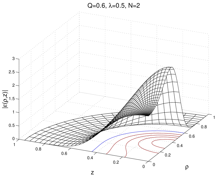
Figure 4: The energy density $\epsilon$ in units of $4\pi\eta/g$ is shown for the dyon solution with topological charge $n=2$, electric charge per topological charge $q_{2}/2=0.6$ and Higgs self-coupling $\lambda=0.5$ as a function of the dimensionless compactified coordinates $\rho=\bar{x}\sin\theta$ and $z=\bar{x}\cos\theta$, where $\bar{x}=x/(1+x)$.

Figure 5: The energy density $\epsilon$ in units of $4\pi\eta/g$ is shown for the dyon solution of Fig. 4 and for the corresponding multimonopole solution as a function of the dimensionless compactified coordinate $\bar{x}$ for several values of the angle $\theta$.

References

-
[1]
G. ‘t Hooft,
Magnetic monopoles in unified gauge theories,
Nucl. Phys. B79 (1974) 276;
A. M. Polyakov, Particle spectrum in quantum field theory, JETP Lett. 20 (1974) 194. - [2] M. K. Prasad and C. M. Sommerfield, Exact classical solution for the ‘t Hooft monopole and the Julia-Zee dyon, Phys. Rev. Lett. 35 (1975) 760.
- [3] E. B. Bogomol’nyi and M. S. Marinov, Sov. J. Nucl. Phys. 23 (1976) 357.
- [4] C. Rebbi and P. Rossi, Multimonopole solutions in the Prasad-Sommerfield limit, Phys. Rev. D22 (1980) 2010.
-
[5]
R. S. Ward,
A Yang-Mills-Higgs monopole of charge 2,
Commun. Math. Phys. 79 (1981) 317;
P. Forgacs, Z. Horvarth and L. Palla, Exact multimonopole solutions in the Bogomolny-Prasad-Sommerfield limit, Phys. Lett. 99B (1981) 232;
Non-linear superposition of monopoles, Nucl. Phys. B192 (1981) 141;
M. K. Prasad, Exact Yang-Mills Higgs monopole solutions of arbitrary charge, Commun. Math. Phys. 80 (1981) 137;
M. K. Prasad and P. Rossi, Construction of exact multimonopole solutions, Phys. Rev. D24 (1981) 2182. - [6] B. Kleihaus, J. Kunz and D. H. Tchrakian, Interaction energy of ’t Hooft-Polyakov monopoles, Mod. Phys. Lett. A13 (1998) 2523.
-
[7]
C. H. Taubes,
The existence of a non-minimal solution
to the SU(2) Yang-Mills-Higgs equations on . Part I,
Commun. Math. Phys. 86 (1982) 257;
Part II, Commun. Math. Phys. 86 (1982) 299. - [8] Bernhard Rüber, Eine axialsymmetrische magnetische Dipollösung der Yang-Mills-Higgs-Gleichungen, Thesis, University of Bonn 1985.
- [9] B. Kleihaus and J. Kunz, A Monopole-Antimonopole Solution of the SU(2) Yang-Mills-Higgs Model, Phys. Rev. D61 (2000) 025003.
-
[10]
see e.g. P. M. Sutcliffe,
BPS Monopoles,
Int. J. Mod. Phys. A12 (1997) 4663;
C. J. Houghton, N. S. Manton and P. M. Sutcliffe, Rational Maps, Monopoles and Skyrmions, Nucl. Phys. B510 (1998) 507. - [11] B. Julia and A. Zee, Poles with both magnetic and electric charges in non-abelian gauge theory, Phys. Rev. D11 (1975) 2227.
-
[12]
F. A. Bais and J. R. Primack,
Integral equations for extended solutions in field theory:
Monopoles and dyons,
Phys. Rev. D13 (1976), 819-829.
Y. Brihaye, B. Kleihaus and D.H. Tchrakian, Dyon-Skyrmion lumps, J. Math. Phys. 40 (1999) 1136. - [13] R. Rajaraman, Solitons and Instantons, North-Holland Publishing Company, 1982. Phys. Rev. D 14 (1976) 1660.
- [14] E. J. Weinberg, Parameter counting for multimonopole solutions, Phys. Rev. D20 (1979) 936.
- [15] S.V. Ketov, Solitons, monopoles and duality: from Sine-Gordon to Seiberg-Witten, Fortsch. Phys. 45 (1997) 237-292.