hep-th/0004096 Bianchi Type I Cosmologies in Arbitrary Dimensional Dilaton Gravities

Abstract

We study the low energy string effective action with an exponential type dilaton potential and vanishing torsion in a Bianchi type I space-time geometry. In the Einstein and string frames the general solution of the gravitational field equations can be expressed in an exact parametric form. Depending on the values of some parameters the obtained cosmological models can be generically divided into three classes, leading to both singular and nonsingular behaviors. The effect of the potential on the time evolution of the mean anisotropy parameter is also considered in detail, and it is shown that a Bianchi type I Universe isotropizes only in the presence of a dilaton field potential or a central deficit charge.

PACS number(s): 04.20.Jb, 04.65.+e, 98.80.-k

I Introduction

In an attempt to address the potential, inherited from string theory, to eliminate the initial cosmological singularity, from which time and our Universe are supposed to have begun about 15 billion years ago, Gasperini and Veneziano initiated a program known as the pre-big bang scenario [1]. The field equations of the pre-big bang cosmology are based on the low energy effective action resulting from string theory. In $D$-dimensions, the massless bosonic fields from the NS-NS sector are the dilaton, $\phi$, the antisymmetric tensor, $B_{\mu\nu}$, and the metric tensor, $\hat{g}_{\mu\nu}$, whose dynamics is described, in the “string frame”, by the following action:

$$\hat{S}=\int d^{D}x\sqrt{-\hat{g}}e^{-2\phi}\left\{\hat{R}+\hat{\kappa}(\hat{\nabla}\phi)^{2}-\frac{1}{12}H_{[3]}^{2}-\hat{U}(\phi)\right\},$$ (1)

where $H_{[3]}=dB_{[2]}$ and $\hat{\kappa}$ is a generalized dilaton coupling constant ($\hat{\kappa}=4$ for superstring theories). Moreover, we also allow for the existence of a potential $\hat{U}(\phi)$ of the dilaton field. From a physical point of view the most important candidate for the potential is a cosmological constant $\Lambda$, which appears in the massive extension of type IIA supergravity and is restricted to be positive, $\Lambda>0$ [4].

For simplicity in the following we shall assume that $H_{[3]}$ is vanishing. In this circumstance, via a conformal rescaling

$$g_{\mu\nu}=e^{-\frac{4}{D-2}\phi}\hat{g}_{\mu\nu},$$ (2)

the action (1) reduces to a $D$-dimensional dilaton gravity whose action, in the “Einstein frame”, has the form

$$S=\int d^{D}x\sqrt{-g}\left\{R-\kappa(\nabla\phi)^{2}-U(\phi)\right\},$$ (3)

with $U(\phi)=e^{\frac{4\phi}{D-2}}\hat{U}(\phi)$ and $\kappa=\frac{4(D-1)}{D-2}-\hat{\kappa}$.

Pre-big bang inflationary cosmological models, based on the actions (1) or (3) have been recently intensively investigated in the physical literature [5, 6, 7, 8, 9, 10, 11, 12]. Gasperini and Ricci [5] have obtained exact solutions to the four-dimensional low energy string effective action adopting a space-independent dilaton and vanishing Kalb-Ramond anti-symmetric tensor fields ansätz for the Bianchi type I, II, III, V, VI₀ and VI_h geometries. They have shown that in such a context the initial curvature singularities can not be avoided. Brandenberger, Easther and Maia [6] have found non-singular spatially homogeneous and isotropic solutions for dilaton gravity in the presence of a special combination of higher derivative terms in the gravitational action. Some of these solutions correspond to a spatially flat, bouncing Universe originating in a dilaton-dominated contracting phase and emerging as an expanding FRW Universe.

Very recently, the string cosmology equations with a dilaton potential have been examined, in the string frame, by Ellis et al. [13], who also give a generic algorithm for obtaining solutions with desired evolutionary properties. The presence of a dilaton potential leads to the violation of the pre-big bang symmetry $a(t)\to 1/a(t)$. Moreover, Garcia de Andrade [14] obtained several classes of solutions of the Einstein-Cartan dilatonic inflationary cosmology. In the cases where the dilatons are constrained by the presence of spin-torsion effects a repulsive gravity is found. The temperature fluctuation has also been computed from the nearly flat spectrum of the gravitational waves produced during inflation, with results agreeing with the COBE data.

Pre-big bang cosmological models, in which there is no need to introduce the inflation or to fine-tune potentials, have many attractive features [15]. Inflation is natural, thanks to the duality symmetries of string cosmology, and the initial condition problem is decoupled from the singularity problem. Finally, quantum instability (pair creation) is able to heat up an initially cold Universe and generate a standard hot big bang with the additional features of homogeneity, flatness and isotropy.

It is the purpose of the present paper to study Bianchi type I cosmological models in the dilaton gravity (1) and (3). More specifically, we shall consider the effects of an exponential type potential, $U(\phi)=U_{0}e^{\lambda\phi}$, with arbitrary values of the constants $U_{0},\lambda$, on the dynamics and evolution of an anisotropic space-time, in both the Einstein and string frames. In this case the general solution of the gravitational field equations can be expressed in an exact parametric form. The physical effects of the potential on the evolution of the anisotropic space-time are also considered in detail.

The present paper is organized as follows. The basic equations describing the dilatonic Bianchi type I cosmological model are obtained in Section 2. The general solution of the field equations for an exponential type dilaton potential is obtained in Section 3 (Einstein frame) and in Section 4 (string frame). In Section 5 we discuss our results and conclusions.

II Einstein Frame Field Equations, Geometry and Consequences

In this paper, we shall consider the $D$-dimensional anisotropic generalization of the flat FRW geometry — the Bianchi type I space-time described by the line-element

$$ds^{2}=-dt^{2}+\sum_{i=1}^{D-1}a_{i}^{2}(t)(dx^{i})^{2}.$$ (4)

For this metric, it is convenient to introduce the following variables: volume scale factor $V$, directional Hubble factors $H_{i}$ and mean Hubble factor $H$ as

$$V := \prod_{i=1}^{D-1}a_{i},$$ (5)

$$H_{i} := \frac{\dot{a}_{i}}{a_{i}},\quad i=1,...,D-1,$$ (6)

$$H := \frac{1}{D-1}\sum_{i=1}^{D-1}H_{i},$$ (7)

$$\Delta H_{i} := H_{i}-H,\quad i=1,...,D-1.$$ (8)

Then one can immediately check out the relation

$$H=\frac{1}{D-1}\frac{\dot{V}}{V}.$$ (9)

In terms of variables (5)-(8) the Ricci tensor of the Bianchi type I geometry can be expressed as

$$R_{00} = -\frac{d}{dt}\sum_{i=1}^{D-1}\left(\frac{\dot{a}_{i}}{a_{i}}\right)-\sum_{i=1}^{D-1}\left(\frac{\dot{a}_{i}}{a_{i}}\right)^{2}$$ (10)

$$= -(D-1)\dot{H}-\sum_{i=1}^{D-1}H_{i}^{2},$$ (11)

$$R_{ii} = a_{i}^{2}\left[\dot{H}_{i}+(D-1)HH_{i}\right],\quad i=1,...,D-1.$$ (12)

On the other hand, the field equations of the action (3) can be achieved by variation with respect to the fields $g^{\mu\nu}$ and $\phi$ giving

$$R_{\mu\nu}-\kappa\nabla_{\mu}\phi\nabla_{\nu}\phi-\frac{U}{D-2}g_{\mu\nu} = 0,$$ (13)

$$\nabla^{2}\phi-\frac{1}{2\kappa}\frac{\partial U}{\partial\phi} = 0,$$ (14)

where $\nabla$ is the covariant derivative of $g_{\mu\nu}$. Thus, for the Bianchi type I space-time, the gravitational field equations in the Einstein frame reduce to

$$(D-1)\dot{H}+\sum_{i=1}^{D-1}H_{i}^{2}+\kappa\dot{\phi}^{2}-\frac{1}{D-2}U=0,$$ (15)

$$\frac{1}{V}\frac{d}{dt}(VH_{i})-\frac{1}{D-2}U = 0,\quad i=1,..,D-1,$$ (16)

$$\frac{1}{V}\frac{d}{dt}(V\dot{\phi})+\frac{1}{2\kappa}\frac{\partial U}{\partial\phi} = 0.$$ (17)

By summing equations (16) we obtain

$$\frac{1}{V}\frac{d}{dt}(VH)=\frac{1}{D-2}U,$$ (18)

which, together with (16), leads to

$$H_{i}=H+\frac{K_{i}}{V},\quad i=1,...,D-1.$$ (19)

In equations (19) $K_{i},i=1,...,D-1$ are constants of integration, which satisfy the relation:

$$\sum_{i=1}^{D-1}K_{i}=0.$$ (20)

Substituting eqs.(19) into (15) and then combining with eq.(18) we obtain

$$\kappa\dot{\phi}^{2}+(D-2)\dot{H}+\frac{K^{2}}{V^{2}}=0,$$ (21)

where $K^{2}:=\sum_{i=1}^{D-1}K_{i}^{2}$. Consequently, the remaining task is to solve the equations (17), (18) and (21).

The physical quantities of interest in cosmology are the expansion scalar $\theta$, the mean anisotropy parameter $A$, the shear scalar $\Sigma^{2}$ and the deceleration parameter $q$ defined according to:

$$\theta := (D-1)H=\frac{\dot{V}}{V},$$ (22)

$$A := \frac{1}{D-1}\sum_{i=1}^{D-1}\left(\frac{\Delta H_{i}}{H}\right)^{2}=\frac{1}{D-1}\frac{K^{2}}{V^{2}H^{2}},$$ (23)

$$\Sigma^{2} := \frac{1}{D-2}\left(\sum_{i=1}^{D-1}H_{i}^{2}-(D-1)H^{2}\right)$$ (24)

$$= \frac{D-1}{D-2}AH^{2},$$ (25)

$$q := \frac{d}{dt}H^{-1}-1.$$ (26)

The sign of the deceleration parameter indicates whether the cosmological model inflates. The positive sign corresponds to standard decelerating models whereas the negative sign indicates inflationary behavior.

III Exponential Potential in the Einstein Frame

The cosmological behavior of Universes filled with scalar field, $\phi$, as well as a Liouville type exponential potential

$$U(\phi)=U_{0}e^{\lambda\phi},$$ (27)

with $U_{0}$ and $\lambda$ constants, has been extensively investigated in the physical literature for both homogeneous and inhomogeneous scalar fields [16]-[28]. An exponential potential arises in the four-dimensional effective Kaluza-Klein type theories from compactification of the higher-dimensional supergravity or superstring theories [2]. A solution in the case of a flat space-time filled with a scalar field with an exponential potential but describing power-law inflationary behavior has been obtained by Barrow [16]. Higher dimensional ($D\geq 4$) anisotropic cosmological models with a massless scalar field self-interacting through an exponential potential have been investigated in [17]. A non-inflationary solution for an open FRW Universe exponential-potential pure scalar field filled space-time and with scalar field energy density decaying as $\rho_{\phi}\sim t^{-2}$ has been recently found by Mubarak and Oezer [25]. In the Einstein frame the exponential potential (27) is also generated by means of the conformal transformation (2) for $\hat{U}(\phi)=\Lambda$, with $\Lambda$ the central charge deficit.

For this type of potential, the combination of equations (16) and (17) leads to

$$\frac{d}{dt}\left(\frac{1}{D-2}V\dot{\phi}+\frac{\lambda}{2\kappa}VH\right)=0,$$ (28)

or, equivalently, to

$$\dot{\phi}=\frac{(D-2)C}{V}-\frac{(D-2)\lambda}{2\kappa}H,$$ (29)

with $C$ a constant of integration.

Substitution of Eq.(29) into Eq.(21) gives the “final” field equation

$$\frac{\ddot{V}}{V}+\alpha\frac{\dot{V}^{2}}{V^{2}}-\beta\frac{\dot{V}}{V^{2}}+\gamma\frac{1}{V^{2}}=0,$$ (30)

where

$$\alpha = \frac{(D-2)\lambda^{2}}{4(D-1)\kappa}-1,$$ (31)

$$\beta = (D-2)C\lambda,$$ (32)

$$\gamma = (D-1)(D-2)C^{2}\kappa+\frac{(D-1)K^{2}}{D-2}.$$ (33)

By introducing a new variable $u:=\dot{V}$, equation (30) takes the form

$$\frac{udu}{-\alpha u^{2}+\beta u-\gamma}=\frac{dV}{V}.$$ (34)

Equation (34) has the general solution (with $V_{0}$ a constant of integration):

$$V=V_{0}\exp\left(\int\frac{udu}{-\alpha u^{2}+\beta u-\gamma}\right).$$ (35)

In the following we shall denote

$$\Delta = \beta^{2}-4\alpha\gamma,$$ (36)

$$u_{0} = \frac{\beta}{2\alpha},$$ (37)

$$u_{\pm} = \frac{\beta\pm\sqrt{\Delta}}{2\alpha},$$ (38)

$$m_{\pm} = -\frac{1}{2\alpha}\left(1\pm\frac{\beta}{\sqrt{\Delta}}\right).$$ (39)

Hence, taking $u$ as a parameter, we obtain three classes of solutions of the gravitational field equations describing a dilaton field filled Bianchi type I pre-big bang Universe. The explicit form of the solutions depends on the values of the parameters $\alpha,\beta$ and $\gamma$. All the solutions are expressed in a closed parametric form and are given by:

A $\Delta>0$

$$t = t_{0}+V_{0}\int(u-u_{+})^{m_{+}-1}(u-u_{-})^{m_{-}-1}du,$$ (40)

$$V = V_{0}(u-u_{+})^{m_{+}}(u-u_{-})^{m_{-}},$$ (41)

$$a_{i} = a_{i0}\prod_{\epsilon=\pm}u^{-\frac{K_{i}m_{\epsilon}}{u_{\epsilon}}}(u-u_{\epsilon})^{(\frac{1}{D-1}+\frac{K_{i}}{u_{\epsilon}})m_{\epsilon}},$$ (42)

$$q = (D-2)+\frac{(D-1)\alpha}{u^{2}}\prod_{\epsilon=\pm}(u-u_{\epsilon}),$$ (43)

$$U = -\frac{(D-2)\alpha}{(D-1)V_{0}^{2}}\prod_{\epsilon=\pm}(u-u_{\epsilon})^{1-2m_{\epsilon}}.$$ (44)

B $\Delta=0$

$$t = t_{0}-\frac{V_{0}}{\alpha}\int(u-u_{0})^{-\frac{1}{\alpha}-2}\exp\left(\frac{u_{0}}{\alpha(u-u_{0})}\right)du,$$ (45)

$$V = V_{0}(u-u_{0})^{-\frac{1}{\alpha}}\exp\left(\frac{u_{0}}{\alpha(u-u_{0})}\right),$$ (46)

$$a_{i} = a_{i0}(u-u_{0})^{-\frac{1}{(D-1)\alpha}}\exp\left(\frac{u_{0}+K_{i}(D-1)}{\alpha(D-1)(u-u_{0})}\right),$$ (47)

$$q = (D-2)+\frac{(D-1)\alpha(u-u_{0})^{2}}{u^{2}},$$ (48)

$$U = -\frac{(D-2)\alpha}{(D-1)V_{0}^{2}}(u-u_{0})^{\frac{2}{\alpha}+2}\exp\left(\frac{-2u_{0}}{\alpha(u-u_{0})}\right).$$ (49)

C $\Delta<0$

$$t = t_{0}+V_{0}\int(-\alpha u^{2}+\beta u-\gamma)^{-\frac{1}{2\alpha}-1}$$ (51)

$$\times\exp\left(-\frac{\beta}{\alpha\sqrt{-\Delta}}\arctan\frac{2\alpha u-\beta}{\sqrt{-\Delta}}\right)du,$$

$$V = V_{0}(-\alpha u^{2}+\beta u-\gamma)^{-\frac{1}{2\alpha}}$$ (53)

$$\times\exp\left(-\frac{\beta}{\alpha\sqrt{-\Delta}}\arctan\frac{2\alpha u-\beta}{\sqrt{-\Delta}}\right),$$

$$a_{i} = a_{i0}(-\alpha u^{2}+\beta u-\gamma)^{-\frac{1}{2\alpha(D-1)}}$$ (55)

$$\times\exp\left(-\frac{\beta+2\alpha K_{i}(D\!-\!1)}{\alpha(D-1)\sqrt{-\Delta}}\arctan\frac{2\alpha u-\beta}{\sqrt{-\Delta}}\right),$$

$$q = (D-2)-(D-1)\frac{-\alpha u^{2}+\beta u-\gamma}{u^{2}},$$ (56)

$$U = \frac{D-2}{(D-1)V_{0}^{2}}(-\alpha u^{2}+\beta u-\gamma)^{\frac{1}{\alpha}+1}$$ (58)

$$\times\exp\left(\frac{2\beta}{\alpha\sqrt{-\Delta}}\arctan\frac{2\alpha u-\beta}{\sqrt{-\Delta}}\right).$$

For all three cases, the quantities $\theta,A$ and $\Sigma^{2}$ can be easily found from

$$\theta=\frac{u}{V},\quad A=\frac{(D-1)K^{2}}{u^{2}},\quad\Sigma^{2}=\frac{K^{2}}{(D-2)V^{2}}.$$ (59)

IV Exponential Potential in the String Frame

In the string frame the gravitational field equations and the dilaton equations are obtained by varying the action (1) and, under the assumption of vanishing $H_{[3]}$, are given by

$$\hat{R}_{\mu\nu}-\frac{1}{2}\hat{g}_{\mu\nu}\hat{R}+2\hat{\nabla}_{\mu}\hat{\nabla}_{\nu}\phi+(\hat{\kappa}-4)\hat{\nabla}_{\mu}\phi\hat{\nabla}_{\nu}\phi$$ (60)

$$-\frac{1}{2}\hat{g}_{\mu\nu}\left\{4\hat{\nabla}^{2}\phi+(\hat{\kappa}-8)(\hat{\nabla}\phi)^{2}-\hat{U}\right\} = 0,$$ (61)

$$\hat{R}+\hat{\kappa}\hat{\nabla}^{2}\phi-\hat{\kappa}(\hat{\nabla}\phi)^{2}-\hat{U}(\phi)+\frac{1}{2}\frac{\partial\hat{U}}{\partial\phi} = 0.$$ (62)

By eliminating $\hat{R}$ between equations (61) and (62), the gravitational field and dilaton equations take the form

$$\hat{R}_{\mu\nu}+2\hat{\nabla}_{\mu}\hat{\nabla}_{\nu}\phi+(\hat{\kappa}-4)\hat{\nabla}_{\mu}\phi\hat{\nabla}_{\nu}\phi\qquad\qquad$$ (63)

$$-\frac{\hat{g}_{\mu\nu}}{2}\left\{(4\!-\!\hat{\kappa})\hat{\nabla}^{2}\phi+2(\hat{\kappa}\!-\!4)(\hat{\nabla}\phi)^{2}-\frac{1}{2}\frac{\partial\hat{U}}{\partial\phi}\right\} = 0,$$ (64)

$$\hat{\nabla}^{2}\phi-2(\hat{\nabla}\phi)^{2}+\frac{4\hat{U}+(D-2)\frac{\partial\hat{U}}{\partial\phi}}{2[(D-2)\hat{\kappa}-4(D-1)]} = 0.$$ (65)

In the present section we shall consider the general solution of equations (61) and (62) for an exponential type potential, $\hat{U}(\phi)=\hat{U}_{0}\exp(\hat{\lambda}\phi)$, with $\hat{\lambda}$ an arbitrary constant. Since the metric tensors are connected via the conformal transformation (2), in the string frame the general solutions of the gravitational field equations can be obtained by applying the conformal transformation (2) to the solution obtained in the Einstein frame. In the string frame we shall also assume an anisotropic Bianchi type I geometry with line element

$$d\hat{s}^{2}=-d\hat{t}^{2}+\sum_{i=1}^{D-1}\hat{a}_{i}^{2}(\hat{t})(dx^{i})^{2},$$ (66)

with the metric tensor components in the two frames connected by the conformal transformation (2) and with the time coordinate $\hat{t}$ defined according to

$$\hat{t}=\int\exp\left[\frac{2}{D-2}\phi(t)\right]dt.$$ (67)

In the two frames the volume scale factor, the directional Hubble factors and the mean Hubble factor are related by means of the general relations:

$$\hat{V} = Ve^{\frac{2(D-1)}{D-2}\phi},$$ (68)

$$\hat{H}_{i} = \left(H_{i}+\frac{2}{D-2}\dot{\phi}\right)e^{-\frac{2}{D-2}\phi},\quad i=1,...,D-1,$$ (69)

$$\hat{H} = \left(H+\frac{2}{D-2}\dot{\phi}\right)e^{-\frac{2}{D-2}\phi}.$$ (70)

To apply the conformal transformation, we need first to find the conformal transformation factor $e^{\phi}$. From equation (18) it is easy to obtain that the potential $U(\phi)$ can be expressed as

$$U(\phi)=\frac{D-2}{D-1}\frac{u}{V^{2}}\left(\frac{d\ln V}{du}\right)^{-1},$$ (71)

leading to

$$e^{\phi}=\left[\frac{D-2}{(D-1)U_{0}}\right]^{\frac{1}{\lambda}}\left(\frac{V^{2}}{u}\frac{d\ln V}{du}\right)^{-\frac{1}{\lambda}}.$$ (72)

Therefore in the string frame the general solution of the gravitational field equation for a dilaton field filled Bianchi type I with an exponential potential of the form

$$\hat{U}(\phi)=U_{0}\exp\left[\left(\lambda-\frac{4}{D-2}\right)\phi\right],$$ (73)

with $\lambda$ an arbitrary constant, can be expressed again in an exact closed parametric form, with $u$ taken as parameter, and is given by

$$\hat{t}-\hat{t}_{0} = \left[\frac{D-2}{(D-1)U_{0}}\right]^{\frac{2}{(D-2)\lambda}}$$ (75)

$$\times\int\left(\frac{V^{2}}{u}\frac{d\ln V}{du}\right)^{1-\frac{2}{(D-2)\lambda}}\frac{du}{V},$$

$$\hat{V}=V\left[\frac{D-2}{(D-1)U_{0}}\right]^{\frac{2(D-1)}{(D-2)\lambda}}\left(\frac{V^{2}}{u}\frac{d\ln V}{du}\right)^{-\frac{2(D-1)}{(D-2)\lambda}},$$ (76)

$$\hat{H} = \left[\frac{D-2}{(D-1)U_{0}}\right]^{-\frac{2}{(D-2)\lambda}}\left(\frac{V^{2}}{u}\frac{d\ln V}{du}\right)^{\frac{2}{(D-2)\lambda}}$$ (78)

$$\times\left[\frac{2C}{V}+\frac{\kappa-\lambda}{(D-1)\kappa}\frac{u}{V}\right],$$

$$\hat{a}_{i} = a_{i0}\left[\frac{D-2}{(D-1)U_{0}}\right]^{\frac{2}{(D-2)\lambda}}\left(\frac{V^{2}}{u}\frac{d\ln V}{du}\right)^{-\frac{2}{(D-2)\lambda}}V^{\frac{1}{D-1}}$$ (80)

$$\;\times\exp\left(K_{i}\int\frac{1}{u}\frac{d\ln V}{du}du\right),\;i=1,...,D-1,$$

$$\hat{A}=(D-1)\sum_{i=1}^{D-1}\left[\frac{\kappa K_{i}}{(\kappa-\lambda)u+2\kappa C(D-1)}\right]^{2},$$ (81)

$$\hat{q}=(D-2)-\frac{u}{D-1}\left(\frac{d\ln V}{du}\right)^{-1}\left[2C+\frac{\kappa-\lambda}{(D-1)\kappa}u\right]^{-2},$$ (82)

$$\hat{U}=U_{0}\left[\frac{D-2}{(D-1)U_{0}}\right]^{1-\frac{4}{(D-2)\lambda}}\left(\frac{V^{2}}{u}\frac{d\ln V}{du}\right)^{\frac{4}{(D-2)\lambda}-1}.$$ (83)

In the string frame there are also three distinct classes of solutions, corresponding to $\Delta>0,\Delta=0$ and $\Delta<0$ respectively. Substituting the values of $V$ obtained in the previous section in the formulae given above, we can find, via straightforward calculations, the explicit parametric representations, for each class of solutions, of the general solution of the gravitational field equations for a dilaton field filled Bianchi type I space-time, with an arbitrary exponential potential.

If in the solution given above we take $\lambda=\frac{4}{D-2}$, we obtain the general solution of the gravitational field equations in the string frame corresponding to a constant potential, or equivalently, to a cosmological constant. In this case also there are three distinct classes of solutions, with all physical quantities represented as exact functions of time. For $\hat{U}(\phi)\equiv\Lambda=const.$, Eq.(75) becomes

$$\hat{t}-\hat{t}_{0}=\sqrt{\frac{D-2}{(D-1)\Lambda}}\int\frac{du}{\sqrt{-\alpha u^{2}+\beta u-\gamma}}.$$ (84)

In order to obtain solutions defined for all values of the parameters we shall assume in the following that $\alpha<0$. Then Eq.(84) has the solutions

$$u = -\frac{\beta}{2|\alpha|}+\delta_{+}\cosh\frac{\hat{t}-\hat{t}_{0}}{\hat{\tau}_{0}},\quad\hbox{for}\quad\Delta>0,$$ (85)

$$u = -\frac{\beta}{2|\alpha|}+\exp\left(\frac{\hat{t}-\hat{t}_{0}}{\hat{\tau}_{0}}\right),\quad\hbox{for}\quad\Delta=0,$$ (86)

$$u = -\frac{\beta}{2|\alpha|}+\delta_{-}\sinh\frac{\hat{t}-\hat{t}_{0}}{\hat{\tau}_{0}},\quad\hbox{for}\quad\Delta<0,$$ (87)

where we denoted $\delta_{\pm}:=\frac{\sqrt{\pm\Delta}}{2|\alpha|}$ and $\hat{\tau}_{0}:=\sqrt{\frac{D-2}{(D-1)\Lambda|\alpha|}}$.

In this way we can obtain the exact (non-parametric) solution for the anisotropic Bianchi type I geometry in the presence of a central charge deficit. We shall not present here the resulting formulae, due to their complicated (but elementary) mathematical form. As compared to the Einstein frame, the evolution of the Universe in the string frame in the presence of the cosmological constant can be quite complicated.

V Discussions and Final Remarks

In order to consider the general effects of a dilaton field potential in the Einstein frame on the dynamics and evolution of an arbitrary dimensional Bianchi type I space-time, we shall also give the general solution of the gravitational field equations (15)-(17) corresponding to $U(\phi)\equiv 0$. In this case we easily obtain:

$$V = V_{0}t,$$ (88)

$$H = \frac{1}{(D-1)t},$$ (89)

$$a_{i} = a_{i0}\;t^{p_{i}},\quad i=1,...,D-1,$$ (90)

$$A = \frac{(D-1)K^{2}}{V_{0}^{2}}=const.,$$ (91)

$$q = D-2=const.,$$ (92)

$$\phi = \phi_{0}\ln t,$$ (93)

where $\phi_{0}=\phi_{0}^{\prime}\sqrt{\frac{1}{\kappa}\left(\frac{D-2}{D-1}-\frac{K^{2}}{V_{0}^{2}}\right)}$, with $\phi_{0}^{\prime}$ a constant of integration. The coefficients $p_{i}:=\frac{1}{D-1}+\frac{K_{i}}{V_{0}}$ satisfy the relations $\sum_{i=1}^{D-1}p_{i}=1$ and $\sum_{i=1}^{D-1}p_{i}^{2}=\frac{1}{D-1}+\frac{K^{2}}{V_{0}^{2}}$. Hence in the Einstein frame the geometry of the potential free dilaton field is of Kasner type, but with $\sum_{i=1}^{D-1}p_{i}^{2}\neq 1$ (if we adopt the normalization $\sum_{i=1}^{D-1}p_{i}^{2}=1$ then we obtain the empty Bianchi type I Universe with $\phi\equiv 0$). The anisotropic Bianchi type I dilaton field filled Universe does not isotropize (the mean anisotropy parameter is a constant for all times) and its evolution is non-inflationary with $q>0$ for all $t$.

In order to analyze the general effects of the dilaton field potential on the dilaton field filled Bianchi type I space-time in the Einstein frame, we shall obtain first the following anisotropy equation:

$$\frac{dA}{dt}=-\frac{2A}{H}\left(\dot{H}+(D-1)H^{2}\right),$$ (94)

which can also be written in the equivalent form

$$\frac{dA}{dt}=-\frac{2AU(\phi)}{(D-2)H},$$ (95)

and integrated to give

$$A(t)=A_{0}\exp\left(-\frac{2}{D-2}\int_{t_{0}}^{t}\frac{U(\phi)}{H}dt\right).$$ (96)

In equation (96) we denoted by $A_{0}$ an arbitrary constant of integration. For $U(\phi)\equiv 0$ we always have $A\equiv A_{0}=const.$ If $\int_{t_{0}}^{t}\frac{U(\phi)}{H}dt$ is a monotonically increasing positive function of time then the presence of the dilaton field potential will lead to the fast isotropization of the Bianchi type I space-time.

In the presence of a potential the deceleration parameter $q=-(\dot{H}+H^{2})/H^{2}$ can be expressed as

$$q=(D-2)-\frac{U(\phi)}{(D-2)H^{2}}.$$ (97)

If $U(\phi)\equiv 0$ in the Einstein frame the evolution of the Universe is non-inflationary, but once the condition $U(\phi)>(D-2)^{2}H^{2}$ is fulfilled, the dynamics of the Bianchi type I space-times becomes inflationary.

In the present paper we have obtained the general solution of the gravitational field equations for a Bianchi type I space-time filled with a dilaton field with an exponential potential in both the Einstein and string frame. In the Einstein frame they describe generically an expanding Universe, with $u=\dot{V}\geq 0$ and with properties strongly dependent on the numerical values of the physical parameters describing the dilaton field and its potential. A contracting Universe with $u=\dot{V}<0$ generally does not satisfy the condition of reality of the scale factors. The solutions of the field equations can be classified into three classes, according to the sign of the quantity $\Delta$. On the other hand for solutions B and C with $\Delta=0$ and $\Delta<0$ respectively, the condition $\alpha<0$ must also be imposed to ensure the positivity of the potential and well-defined physical quantities for all time. In the limit of large $u$, $u\to\infty$, all three solutions have a similar behavior. The mean anisotropy $A$ tends in all cases to zero, indicating that an exponential type potential leads to the isotropization of the Universe. In the large $u$ limit the deceleration parameter behaves as $q=(D-2)+\alpha(D-1)$. If the condition $\alpha<-\frac{D-2}{D-1}$, or, equivalently, $\lambda^{2}<\frac{4\kappa}{D-2}$ is fulfilled, the Universe will enter in an inflationary phase. For values of $\alpha$ which do not satisfy this condition the evolution of the space-time will be generally non-inflationary. In the same limit of large $u$ the scalar field is given by $\phi\sim\frac{\alpha+1}{\alpha}\ln u$.

For class A solutions, the Bianchi type I dilaton field filled Universe starts in the Einstein frame from a singular state, corresponding to the values $u=u_{+}$ or $u=u_{-}$ of the parameter. Hence for this model a singular state with zero values of the scale factors is unavoidable. But for class B of solutions the evolution of the Universe is non-singular for $u_{0}<0$. In this case the scale factors are finite for all finite values of the parameter $u$. Alternatively, class C models are non-singular for values of the constants $\alpha$ and $\gamma$ such that $\alpha<0$ and $\gamma<0$.

FIG. 1.: Time evolution in the Einstein frame of the four-dimensional ($D=4$) volume scale factor $V(t)$ of the dilaton field filled Bianchi type I Universe with exponential potential for different values of the parameters $\alpha,\beta$ and $\gamma$: (i). Class A Model (full curve) $\alpha=-\frac{1}{3},\beta=1,\gamma=1$, (ii). Class B Model (dotted curve) $u_{0}=1$ and (iii). Class C Model (dashed curve) $\alpha=-\frac{1}{3},\beta=1,\gamma=-1$.

FIG. 2.: Einstein frame time evolution of the four-dimensional mean anisotropy parameter $a(t):=\frac{A(t)}{3K^{2}}$ of the dilaton field filled Bianchi type I Universe with exponential potential for different values of the parameters $\alpha,\beta$ and $\gamma$: (i). Class A Model (full curve) $\alpha=-\frac{1}{3},\beta=1,\gamma=1$, (ii). Class B Model (dotted curve) $u_{0}=1$ and (iii). Class C Model (dashed curve) $\alpha=-\frac{1}{3},\beta=1,\gamma=-1$. An expanding Bianchi type I Universe always isotropizes in the presence of an exponential dilaton potential.

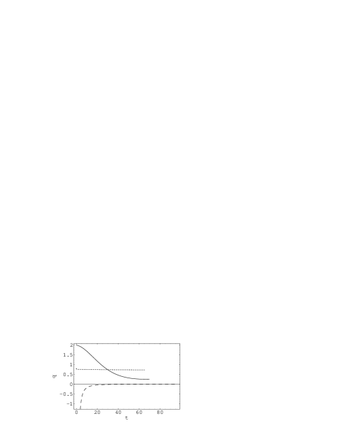
FIG. 3.: Dynamics of the four-dimensional ($D=4$) deceleration parameter $q(t)$ of the dilaton field filled Bianchi type I Universe with exponential potential, in the Einstein frame, for different values of the parameters $\alpha,\beta$ and $\gamma$: (i). Class A Model (full curve) $\alpha=-\frac{1}{3},\beta=1,\gamma=1$, (ii). Class B Model (dotted curve) $u_{0}=1$ and (iii). Class C Model (dashed curve) $\alpha=-\frac{1}{3},\beta=1,\gamma=-1$. Depending on the values of the parameters the Bianchi type Universe has both inflationary and non-inflationary evolutions.

FIG. 4.: Variation in the Einstein frame of the four-dimensional ($D=4$) dilaton field $\phi(t)$ for different values of the parameters $\alpha,\beta$ and $\gamma$: (i). Class A Model (full curve) $\alpha=-\frac{1}{3},\beta=1,\gamma=1$, (ii). Class B Model (dotted curve) $u_{0}=1$ and (iii). Class C Model (dashed curve) $\alpha=-\frac{1}{3},\beta=1,\gamma=-1$.

In Figs. 1-4 we have represented the variations in the Einstein frame of the volume scale factor, mean anisotropy, deceleration parameter and dilaton field for a four-dimensional ($D=4$) Bianchi type I space-time. The anisotropic Universe will always end in an isotropic state, but its dynamics can be either inflationary or non-inflationary. Generally the dilaton field $\phi$ is a decreasing function of time.

We shall consider now the effects of the dilaton field and potential on the dynamics and evolution of a Bianchi type I space-time in the string frame. In the case in which there is no dilaton field potential, $\hat{U}(\phi)\equiv 0$, the general solution of the gravitational field equations and of the dilaton equation can be obtained again by the conformal transformation (2) from (89-93). Hence in this case we obtain first the relation connecting the time coordinate in the string and Einstein frames in the form

$$t=\left(\frac{\hat{t}}{\hat{n}}\right)^{\hat{n}},$$ (98)

where

$$\hat{n}=\frac{D-2}{D-2+2\phi_{0}},$$ (99)

In the string frame the general solution of the potential free dilaton field filled anisotropic Universe is given by

$$\hat{V} = \hat{V}_{0}\hat{t}^{\hat{h}},$$ (100)

$$\hat{H} = \frac{\hat{h}}{(D-1)\hat{t}},$$ (101)

$$\hat{a}_{i} = \hat{a}_{i0}\hat{t}^{\hat{p}_{i}},\quad i=1,...,D-1,$$ (102)

and

$$\hat{A} := \frac{1}{D-1}\sum_{i=1}^{D-1}\left(\frac{\Delta\hat{H}_{i}}{\hat{H}}\right)^{2}$$ (103)

$$= \frac{1}{D-1}\sum_{i=1}^{D-1}\left[1-\frac{(D-1)\hat{p}_{i}}{\hat{h}}\right]^{2},$$ (104)

$$\hat{q} = \frac{D-1}{\hat{h}}-1,$$ (105)

where $\hat{V}_{0}$ and $\hat{a}_{i0}$ are arbitrary constants of integration. Here we also denoted

$$\hat{h} = \frac{D-2+2(D-1)\phi_{0}}{D-2+2\phi_{0}},$$ (106)

$$\hat{p}_{i} = \hat{n}\left(p_{i}+\frac{2\phi_{0}}{D-2}\right),\quad i=1,...,D-1,$$ (107)

and the coefficients $\hat{p}_{i}$ satisfy the relations

$$\sum_{i=1}^{D-1}\hat{p}_{i} = \hat{n}\left[1+\frac{2(D-1)}{D-2}\phi_{0}\right],$$ (108)

$$\sum_{i=1}^{D-1}\hat{p}_{i}^{2} = \hat{n}^{2}\left[\frac{1}{D\!-\!1}+\frac{K^{2}}{V_{0}^{2}}+\frac{4\phi_{0}}{D\!-\!2}\left(1+\frac{D\!-\!1}{D-2}\phi_{0}\right)\right].$$ (109)

In the string frame the general physical behavior of the potential free dilatonic Bianchi type I Universe is quite similar to that in the Einstein frame. The geometry is of the Kasner type, with a power-law type time dependence of the scale factors. The mean anisotropy of the space-time is constant and the Universe will never isotropize. On the other hand if the condition $\hat{h}>D-1$ is fulfilled, the Universe experiences an eternal power law type inflationary anisotropic phase. Hence in the string frame a dilaton field filled Bianchi type I Universe provides an example of an inflating but never isotropizing cosmological type evolution.

In the string frame and in the presence of an exponential potential $\hat{U}(\phi)=\hat{U}_{0}\exp\left(\hat{\lambda}\phi\right)$, with $\hat{\lambda}=\lambda-\frac{4}{D-2}$ and $\lambda$ an arbitrary constant, the Bianchi type I Universe shows a very large variety of behaviors. In Figs.5-8 we represented the dynamics of the volume scale factor, anisotropy parameter, deceleration parameter and potential for different values of $\lambda$ (different exponential potential functions) but for fixed $\alpha,\beta$ and $\gamma$. These solutions generically begin from a singular state, followed by an expansionary phase, with the volume scale factor and scale factors reaching a local maximum. Then the Universe re-collapse into a new singular phase. This type of evolution is associated with an initial rapid isotropization of the space-time, with the mean anisotropy parameter $\hat{A}$ rapidly decreasing. Near the second singular state the evolution of the Universe is generally inflationary, with the string frame deceleration parameter $\hat{q}$ smaller than zero, $\hat{q}<0$. After this phase the effect of the dilaton becomes irrelevant to the dynamics of space-time.

FIG. 5.: String frame evolution of the volume scale factor $\hat{V}$ of the dilatonic Bianchi type I Universe in the presence of an exponential potential $\hat{U}=U_{0}\exp\left[\left(\lambda-\frac{4}{D-2}\right)\phi\right]$ as a function of time $\hat{t}$ for $\alpha=-1/3$, $\beta=1$, $\gamma=1$ and for different values of $\lambda$: $\lambda=3$ (full curve), $\lambda=2$ (this case corresponds to the presence of a central charge deficit or cosmological constant) (dotted curve) and $\lambda=1$ (dashed curve). We have used the normalization $\frac{D-2}{(D-1)U_{0}}=1$.

FIG. 6.: Time variation of the anisotropy parameter $\hat{A}$ in the string frame for $\alpha=-1/3$, $\beta=1$, $\gamma=1$ and for different values of $\lambda$: $\lambda=3$ (full curve), $\lambda=2$ (this case corresponds to the presence of a central charge deficit or cosmological constant) (dotted curve) and $\lambda=1$ (dashed curve). We have used the normalization $\frac{D-2}{(D-1)U_{0}}=1$.

FIG. 7.: Dynamics of the deceleration parameter $\hat{q}$ in the string frame in the presence of the exponential potential $\hat{U}=U_{0}\exp\left[\left(\lambda-\frac{4}{D-2}\right)\phi\right]$, $\alpha=-1/3$, $\beta=1$, $\gamma=1$ and $\lambda=3$ (full curve), $\lambda=2$ (this case corresponds to the presence of a central charge deficit or cosmological constant) (dotted curve) and $\lambda=1$ (dashed curve). We have used the normalization $\frac{D-2}{(D-1)U_{0}}=1$.

FIG. 8.: Time evolution in the string frame of the exponential potential $\hat{U}=U_{0}\exp\left[\left(\lambda-\frac{4}{D-2}\right)\phi\right]$ for $\alpha=-1/3$, $\beta=1$, $\gamma=1$ and $\lambda=3$ (full curve), $\lambda=2$ (this case corresponds to a constant potential $\hat{U}=const.$) (dotted curve) and $\lambda=1$ (dashed curve). We have used the normalization $\frac{D-2}{(D-1)U_{0}}=1$.

In the limit of large values of the parameter $u$, the term $-\alpha u^{2}$ dominates, $-\alpha u^{2}>>\beta u-\gamma$. Hence in the limit of large $u$ (and large time, $\hat{t}\to\infty$, too), from equation (35) we obtain $V\simeq V_{0}u^{-\frac{1}{\alpha}}$. Therefore from Eq.(75) it follows that $\hat{t}\simeq u^{(1+1/\alpha)(4/(D-2)\lambda-1)}\simeq u^{1/\hat{l}}$, and, consequently,

$$\hat{V} \simeq \hat{t}^{(D-1)\hat{l}^{\prime}},$$ (110)

$$\hat{H} \simeq \hat{t}^{-1},$$ (111)

$$\hat{a}_{i} \simeq \hat{t}^{\hat{l}^{\prime}}\exp\left(\frac{V_{0}K_{i}}{\alpha}\hat{t}^{-\hat{l}}\right),\quad i=1,...,D-1,$$ (112)

$$\hat{A} \simeq \hat{t}^{-2\hat{l}},$$ (113)

$$\hat{q} \simeq (D-2)+\frac{(D-1)\alpha\kappa^{2}}{V_{0}(\kappa-\lambda)^{2}},$$ (114)

$$\hat{U} \simeq \hat{t}^{-2},$$ (115)

where we denoted

$$\hat{l} = \frac{1}{\left(1+\frac{1}{\alpha}\right)\left[\frac{4}{(D-2)\lambda}-1\right]},$$ (116)

$$\hat{l}^{\prime} = 1+\hat{l}\left[1+\frac{D-2}{(D-1)\alpha}\right].$$ (117)

In the long-time limit the behavior of the exponential potential dilaton field filled Universe is quite different to the behavior of the potential free dilatonic anisotropic Universe. The dependence of the coefficients $\hat{l},\hat{l}^{\prime}$ on the two constants $\alpha$ and $\lambda$ leads to a larger spectrum of admissible final states, with isotropic inflationary or non-inflationary evolution or re-collapse into a singular state. For $|\alpha|<1$ generally $\hat{l}<0$, and, if $\hat{l}<-\left(1+\frac{D-2}{(D-1)\alpha}\right)^{-1}$, then the volume scale factor tends to zero in the string frame, $\hat{V}\to 0$.

It is well known that the action (1) with vanishing antisymmetric field strength $H_{[3]}$ is invariant with respect to scale factor duality transformations of the form $G\to\bar{G}=G^{-1}$ and $\phi\to\bar{\phi}-\ln(\det G)$, where $G$ is a matrix build from the metric tensor components of the FRW, anisotropic or inhomogeneous metric [9]. The inclusion of the potential breaks this duality, but leads, on the other hand, to the possibility of obtaining more general models allowing a better physical description of the very early evolution of our Universe.

REFERENCES

[1]
M. Gasperini and G. Veneziano,
Pre-Big Bang in String Cosmology,
Astropart. Phys. 1 (1993) 317-339;
hep-th/9211021.
[2]
C.G. Callan, E.J. Martinec, M.J. Perry and D.Friedan,
Strings in Background Fields,
Nucl. Phys. B262 (1985) 593-609.
[3]
C. Lovelace,
Stability of String Vacua. 1. A New Picture of the
Renormalization Group,
Nucl. Phys. B273 (1986) 413-467.
[4]
L.J. Romans,
Massive Supergravity in Ten-Dimensions,
Phys. Lett. B169 (1986) 374-380.
[5]
M. Gasperini and R. Ricci,
Homogeneous Conformal String Backgrounds,
Class. Quant. Grav. 12 (1995) 677-688;
hep-th/9501055.
[6]
R. Brandenberger, R. Easther and J. Maia,
Non-singular Dilaton Cosmology,
JHEP 9809 (1998) 007;
gr-qc/9806111.
[7]
A.L. Maroto and I.L. Shapiro,
On the Inflationary Solutions in Higher Derivative Gravity
with Dilaton Field,
Phys. Lett. B414 (1997) 34-44;
hep-th/9706179.
[8]
R. Easther, K. Maeda and D. Wands,
Tree Level String Cosmology,
Phys. Rev. D53 (1996) 4247-4256;
hep-th/9509074.
[9]
E. Di Pietro and J. Demaret,
Scale Factor Duality in String Bianchi Cosmologies,
Int. J. Mod. Phys. D8 (1999) 349-361;
gr-qc/9903063.
[10]
A. Lukas, B.A. Ovrut and D. Waldram,
The Cosmology of M-Theory and Type II Superstrings,
hep-th/9802041.
[11]
M. Gasperini,
Elementary Introduction to Pre-Big Bang Cosmology and to the
Relic Graviton Background,
hep-th/9907067.
[12]
E.J. Copeland, A. Lahiri and D. Wands,
Low Energy Effective String Cosmology,
Phys. Rev. D57 (1994) 4868-4880;
hep-th/9406216.
[13]
G.F.R. Ellis, D.C. Roberts, D. Solomons and P.K.S. Dunsby,
Using the Dilaton Potential to Obtain String Cosmology Solutions,
gr-qc/9912005.
[14]
L.C. Garcia de Andrade,
On Dilaton Solutions of de Sitter Inflation and Primordial
Spin Torsion Density Fluctuations,
gr-qc/9906085.
[15]
G. Veneziano,
A Simple/Short Introduction to Pre-Big Bang Physics/Cosmology,
hep-th/9802057.
[16]
J.D. Barrow,
Cosmic No Hair Theorems and Inflation,
Phys. Lett. B187 (1987) 12-16.
[17]
J.M. Aguirregabiria, A. Feinstein, and J. Ibanez,
Exponential Potential Scalar Field Universes.
1. The Bianchi Type I Models,
Phys. Rev. D48 (1993) 4662-4668;
gr-qc/9309013.
[18]
J.M. Aguirregabiria, A. Feinstein, and J. Ibanez,
Exponential Potential Scalar Field Universes.
2. The Inhomogeneous Models,
Phys. Rev. D48 (1993) 4669-4675;
gr-qc/9309014.
[19]
A. Feinstein, J. Ibanez and P. Labraga,
Scalar Field Inhomogeneous Cosmologies,
J. Math. Phys. 36 (1995) 4962-4974;
gr-qc/9511066.
[20]
L.P. Chimento and A.S. Jakubi,
Scalar Field Cosmologies with Perfect Fluid
in Robertson-Walker Metric,
Int. J. Mod. Phys. D5 (1996) 71-84;
gr-qc/9506015.
[21]
J. Ibanez and I. Olasagasti,
Asymptotic Behavior of a Class of Inhomogeneous Scalar Field
Cosmologies,
J. Math. Phys. 37 (1996) 6283-6292;
gr-qc/9607062.
[22]
A.A. Coley, J. Ibanez and R.J. van den Hoogen,
Homogeneous Scalar Field Cosmologies with
an Exponential Potential,
J. Math. Phys. 38 (1997) 5256-5271.
[23]
E.J. Copeland, A.R. Liddle and D. Wands,
Exponential Potentials and Cosmological Scaling Solutions,
Phys. Rev. D57 (1998) 4686-4690;
gr-qc/9711068.
[24]
A.P. Billyard, A.A. Coley and R.J. van den Hoogen,
The Stability of Cosmological Scaling Solutions,
Phys. Rev. D58 (1998) 123501;
gr-qc/9805085.
[25]
K.M. Mubarak and M. Oezer,
Singular Scalar Field Cosmologies with Energy Density
Decaying ,
Class. Quant. Grav. 15 (1998) 75-88.
[26]
M. Susperregi and A. Mazumdar,
Extended Inflation with an Exponential Potential,
Phys. Rev. D58 (1998) 083512;
gr-qc/9804081.
[27]
J. Ibanez and I. Olasagasti,
On the Evolution of a Large Class of Inhomogeneous Scalar
Field Cosmologies,
Class. Quant. Grav. 15 (1998) 1937-1950;
gr-qc/9803078.
[28]
S. Byland and D. Scialom,
Evolution of the Bianchi I, the Bianchi III and
the Kantowski-Sachs Universe: Isotropization and Inflation,
Phys. Rev. D57 (1998) 6065-6074;
gr-qc/9802043.