KEK-TH-683

KUNS-1655

April 2000

String Scale in Noncommutative Yang-Mills

Nobuyuki Ishibashi¹⁾, Satoshi Iso¹⁾, Hikaru Kawai²⁾and Yoshihisa Kitazawa¹⁾

¹⁾ Laboratory for Particle and Nuclear Physics,
High Energy Accelerator Research Organization (KEK),
Tsukuba, Ibaraki 305-0801, Japan

²⁾ Department of Physics, Kyoto University, Kyoto 606-8502, Japan

We identify the effective string scale of noncommutative Yang-Mills theory (NCYM) with the noncommutativity scale through its dual supergravity description. We argue that Newton’s force law may be obtained with 4 dimensional NCYM with maximal SUSY. It provides a nonperturbative compactification mechanism of IIB matrix model. We can associate NCYM with the von Neumann lattice by the bi-local representation. We argue that it is superstring theory on the von Neumann lattice. We show that our identification of its effective string scale is consistent with exact T-duality (Morita equivalence) of NCYM.

1 Introduction

In recent studies of nonperturbative aspects of superstring theory, type IIB superstring is found to provide the simplest setting[1][2]. However it is difficult to obtain a realistic unified theory in IIB superstring at least perturbatively. Therefore we may expect that an entirely new type of nonperturbative compactification mechanism of IIB superstring exits[3][4]. On the other hand, a new compactification mechanism which involves branes has been proposed[5]. Since branes naturally appear in superstring theory[6], such a mechanism is expected to apply for IIB superstring theory.

Noncommutative Yang-Mills theory (NCYM) has been obtained by compactifying IIB matrix model on noncommutative tori[7]. We can simply obtain $\tilde{d}$ dimensional NCYM by expanding IIB matrix model around $\tilde{d}$ dimensional noncommuting backgrounds[8]. In IIB matrix model, the dynamical variables are the Hermitian matrices which are interpreted as the space-time coordinates. A $\tilde{d}$ dimensional noncommuting background corresponds to a $\tilde{d}$ dimensional noncommutative space-time. The simplest idea for compactification in IIB matrix model is to postulate that the compactification down to $\tilde{d}$ dimensions is realized by expanding the model around $\tilde{d}$ dimensional backgrounds.

In this paper we point out that Newton’s force law may be obtained with four dimensional NCYM with maximal SUSY ($NCYM_{4}$). Our argument is based on its dual supergravity description[9][10]. We argue that there exists a massless bound state in the effective Hamiltonian of supergravity which gives rise to Newton’s force law a la Randall and Sundrum. Therefore $NCYM_{4}$ may be regarded as a four dimensional compactification of IIB superstring. The remarkable feature is that it compactifies ten dimensional superstring straight down to four dimensions. The compactification of matrix models has been the outstanding problem[11][12]. We argue that we can obtain four dimensional gauge theory and gravitation with four dimensional noncommutative backgrounds in IIB matrix model. In this sense, we have identified the most satisfactory compactification mechanism of matrix models. It is also possible to obtain $d+1$ dimensional NCYM theories by expanding BFSS matrix model around $d$ dimensional noncommutative backgrounds in an analogous way. It may be interesting to investigate such theories through supergravity approach. However it is beyond the scope of this paper.

In the large $N$ expansion of gauge theory, Feynman diagrams can be classified with their world sheet topology. This is a generic feature of matrix valued field theory. On the other hand, string theory is perturbatively defined in terms of field theory on the world sheet. String theory may be nonperturbatively formulated in the large $N$ limit of matrix models in view of these remarkable correspondences. IIB matrix model is such a proposal which is a large $N$ reduced model of maximally supersymmetric gauge theory[1]:

$$S=-{1\over g^{2}}Tr({1\over 4}[A_{\mu},A_{\nu}][A^{\mu},A^{\nu}]+{1\over 2}\bar{\psi}\Gamma^{\mu}[A_{\mu},\psi]).$$ (1.1)

Here $\psi$ is a ten dimensional Majorana-Weyl spinor field, and $A_{\mu}$ and $\psi$ are $N\times N$ Hermitian matrices.

With vanishing fermionic backgrounds, the equations of motion are:

$$[A_{\mu},[A_{\mu},A_{\nu}]]=0.$$ (1.2)

The following solutions correspond to BPS-saturated backgrounds:

$$[A_{\mu},A_{\nu}]=c-number\equiv C_{\mu\nu}.$$ (1.3)

Since we interpret $A_{\mu}$ as space-time coordinates due to $\cal{N}$=2 SUSY, we expect to obtain $\tilde{d}$ dimensional space-time with $\tilde{d}$ dimensional solutions of this type. We further expect to obtain $\tilde{d}$ dimensional gauge theory. Since matrices form noncommutative but associative algebra, we expect a deep connection to noncommutative geometry [13]. In fact we have obtained NCYM of 16 supercharges with these backgrounds[8]. Ordinary gauge theory appears as the low energy effective theory. Since short open strings correspond to gauge particles, we indeed find another evidence that IIB matrix model can describe infinite numbers of fundamental strings. We have further pointed out that NCYM contains nonlocal degrees of freedom which may be interpreted as long open strings[14][15]. We have indeed shown that they give rise to gravitational interactions at the one loop level as it is expected in superstring theory[8][15].

Since NCYM seems to contain the both gauge theory and gravitation, it is very likely that it is equivalent to superstring theory in a particular background. The major issue here is the renormalizability of NCYM [30][31]. We have shown that the high energy behavior of NCYM is equivalent to large $N$ gauge theory by using the bi-local field representation[15]. Although it also exhibits long range interactions which we interpret as gravitation, it is very likely that NCYM exits at least for $\tilde{d}\leq 4$.

NCYM is often argued to be the low energy limit of string theory with constant $b_{\mu\nu}$ field [16][17][18] [19][20] . However long range interactions are found due to the presence of long ‘open strings’ which might signal the presence of ‘closed strings’ [8][15][31][32][33][34]. These issues are currently under active investigations [40][41][42][43][44]. In this paper we propose that NCYM is superstring theory on the von Neumann lattice whose effective string scale $\alpha^{\prime}_{eff}$ is set by $C_{\mu\nu}$.

The organization of this paper is as follows. In section 2, we argue that Newton’s force law is obtained with $NCYM_{4}$. Since it is a nonperturbative problem, we study its dual supergravity description. In section 3, we briefly summarize our formulation of NCYM as twisted reduced models. In section 4, we estimate the string tension of NCYM using the formalism of section 3. We find that our estimate is consistent with string theoretic expectations in section 2. In section 5, we investigate the graviton exchange process by the one loop perturbation theory. We conclude in section 6 with discussions.

2 $NCYM_{4}$ as a unified theory

In this section, we argue that $NCYM_{4}$ contains four dimensional gauge theory and gravitation. It is clear that NCYM contains ordinary gauge theory since the noncommutative phases become ineffective at tree level in the low energy limit. The remarkable possibility is that it may also contain gravitation. We first observe the long range interaction at the one loop level which is specific in NCYM. It can be interpreted as gravitational interaction in IIB superstring as it is explained in section 5. In string theory, closed string exchanges should be visible at open string one loop level. Therefore this phenomenon is another stringy feature of NCYM. Although we can see the glimpse of closed strings at the one loop level, we need to understand the quantum effects to all orders to investigate the gravitational sector of $NCYM_{4}$.

In order to study such a problem, we recall the supergravity solution of $m$ coincident D3-branes with the constant NS B field strength $b$[10]:

$$e^{\phi} = g_{\infty}{(1+{g_{\infty}m\alpha^{\prime 2}(1+\alpha^{\prime 2}b^{2})\over r^{4}})\over(1+{g_{\infty}m\alpha^{\prime 2}\over r^{4}})},$$

$${1\over\alpha^{\prime}}ds^{2} = {1\over\alpha^{\prime}}(1+{g_{\infty}m\alpha^{\prime 2}(1+\alpha^{\prime 2}b^{2})\over r^{4}})^{1\over 2}({d\vec{x}^{2}\over 1+{g_{\infty}m\alpha^{\prime 2}\over r^{4}}}+dr^{2}+r^{2}d\Omega_{5}^{2}),$$

$$B_{2} = {b\over(1+{g_{\infty}m\alpha^{\prime 2}\over r^{4}})}dx\wedge dy+{b\over(1+{g_{\infty}m\alpha^{\prime 2}\over r^{4}})}dz\wedge d\tau,$$

$$C_{2} = i{1\over g_{\infty}(1+\alpha^{\prime 2}b^{2})}B_{2},$$

$$C_{0} = -i{b^{2}\over g_{\infty}(1+\alpha^{\prime 2}b^{2})}{1\over(1+{g_{\infty}m(1+\alpha^{\prime 2}b^{2})\over r^{4}})},$$

$$F_{0123r} = -4i{1\over(1+{g_{\infty}m\alpha^{\prime 2}\over r^{4}})^{2}}{{m\over r^{5}}}.$$ (2.1)

Here $g_{\infty}$ is the dilaton expectation value at $r={\infty}$. $\vec{x}$ denotes four dimensional space-time coordinates in this section.

These background fields appear in the Euclidean IIB supergravity action:

$$S_{IIB} = S_{NS}+S_{R}+S_{CS},$$

$$S_{NS} = -{1\over 2}\int d^{10}x\sqrt{g}e^{-2\phi}(R+4\partial_{\mu}\phi\partial^{\mu}\phi-{1\over 2}{H_{3}}^{2}),$$

$$S_{R} = {1\over 4}\int d^{10}x\sqrt{g}({F_{1}}^{2}+{\tilde{F}_{3}}^{2}+{1\over 2}{\tilde{F}_{5}}^{2}),$$

$$S_{CS} = {1\over 4}\int C_{4}\wedge H_{3}\wedge F_{3},$$ (2.2)

where

$$\tilde{F}_{3} = F_{3}-C_{0}\wedge H_{3},$$

$$\tilde{F}_{5} = F_{5}-{1\over 2}C_{2}\wedge H_{3}+{1\over 2}B_{2}\wedge F_{3}.$$ (2.3)

We identify the $r$ dependent metric $g_{\alpha\beta}$ in eq.(2.1) as the four dimensional metric for fundamental strings:

$$g_{\alpha\beta}=(1+{g_{\infty}m\alpha^{\prime 2}(1+\alpha^{\prime 2}b^{2})\over r^{4}})^{1\over 2}({1\over 1+{g_{\infty}m\alpha^{\prime 2}\over r^{4}}})\delta_{\alpha\beta}.$$ (2.4)

We postulate that D3-branes are located at the maximum of $g_{\alpha\beta}$ , namely at the ‘boundary’ $r=(g_{\infty}m\alpha^{\prime 2})^{1/4}$. Since open strings live on the D3-branes, we identify the open string metric $G_{\alpha\beta}$ with $g_{\alpha\beta}$ at the ‘boundary’ as

$$G_{\alpha\beta}\sim(1+\alpha^{\prime 2}b^{2})^{1\over 2}\delta_{\alpha\beta}.$$ (2.5)

Eq.(2.1) indicates that fundamental string metric grows at smaller $r$. This phenomenon may be interpreted that closed strings become dynamical due to the quantum effects in NCYM. The graviton exchanges we find at the one loop level in section 5 support such an interpretation. We consider the case that the noncommutativity scale $l_{NC}$ is much smaller than the string scale $l_{s}$. Let us focus on the physics at the noncommutativity scale by letting $\alpha^{\prime}\rightarrow\infty$ but keeping $b,r\sim O(1)$. Although it might appear to be a strange limit, it is equivalent to consider the standard $\alpha^{\prime}\sim\epsilon^{1/2},x_{\mu}\sim\epsilon^{1/2}\tilde{x}_{\mu},b\sim\epsilon^{-1}$ limit. The remarkable point is that open string metric is given by eq.(2.5) as $\alpha^{\prime}b$ in this limit.

The Polyakov action for fundamental strings becomes in such a limit as

$${1\over\alpha^{\prime}}\int d^{2}zG_{\alpha\beta}\partial x^{\alpha}\bar{\partial}x^{\beta}+\int d^{2}zb_{\alpha\beta}\partial_{0}x^{\alpha}\partial_{1}x^{\beta}+\cdots$$ (2.6)

$$\sim {b}\int d^{2}z(\partial_{0}x_{\alpha}\partial_{0}x^{\alpha}-\partial_{1}x_{\alpha}\partial_{1}x^{\alpha})+\int d^{2}zb_{\alpha\beta}\partial_{0}x^{\alpha}\partial_{1}x^{\beta}+\cdots.$$

So the Hamiltonian for open strings behaves like

$$cp^{2}+\sum_{k\neq 0}kn_{k},$$ (2.7)

where $c=1/b$ and $n_{k}$ denote the number operators of the oscillator modes. Here we find that the noncommutativity scale now acts as the effective string scale!

Supergravity description of $U(m)$ $NCYM_{4}$ may be obtained by considering large $\alpha^{\prime}$ and small $g_{\infty}$ limit while keeping $\lambda=g_{\infty}\alpha^{\prime 2}b^{2}$ fixed[10]:

$$e^{\phi} = ({m\lambda^{2}\over r^{4}}){1\over(1+{m\lambda\over r^{4}})},$$

$${1\over\alpha^{\prime}}ds^{2} = ({m\lambda\over r^{4}})^{1\over 2}({d\vec{x}^{2}\over 1+{m\lambda\over r^{4}}}+dr^{2}+r^{2}d\Omega_{5}^{2}),$$

$$B_{2} = {1\over(1+{m\lambda\over r^{4}})}dx\wedge dy+{1\over(1+{m\lambda\over r^{4}})}dz\wedge d\tau,$$

$$C_{2} = i{1\over\lambda}B_{2},$$

$$C_{0} = -i{r^{4}\over m\lambda^{2}},$$

$$F_{0123r} = -4i{1\over(1+{m\lambda\over r^{4}})^{2}}{m\over r^{5}}.$$ (2.8)

Here we have also put $b=1$ which implies that the noncommutativity scale $l_{NC}$ is $O(1)$. Since we are looking at the vicinity of the D3-branes in this limit, we expect to find massless open strings. However we also find oscillator modes since the effective string scale is set by $l_{NC}$ as in eq.(2.7).

We recall that there is a crossover at the noncommutativity scale $l_{NC}$ in NCYM. When we consider the Wilson loops, we find that the planar diagrams dominate at larger momentum scale than $1/l_{NC}$ and the diagrams of all topology contribute in the opposite limit[24]. It may be interpreted that the string coupling (dilaton expectation value) is scale dependent. It is because in our IIB matrix model conjecture, the tree level string theory is considered to be obtained by summing planar diagrams and string perturbation theory is identified with the topological expansion of the matrix model. With this interpretation, the string coupling grows as the relevant momentum scale is decreased while it vanishes in the opposite limit. In the $D$ brane interpretation, the small momentum region corresponds to the vicinity of the brane, while the large momentum region corresponds to the region far from the brane since the Higgs expectation value plays the same role with the momentum scale. In this sense $e^{\phi}$ in eq.(2.8) behaves just like the $NCYM_{4}$ [14][31].

The small $r$ behavior of eq.(2.8) is identical with ordinary $AdS$/CFT correspondence if we identify $\lambda$ as the coupling of ordinary Yang-Mills theory[2]. This result is reasonable since the low energy limit of $NCYM_{4}$ contains ordinary gauge theory with precisely the same relation between the coupling constants. It is because in string theory the coupling of $NCYM_{4}$ is given by $\lambda=g_{\infty}\alpha^{\prime}b^{2}$ when $\alpha^{\prime}$ is large.

We may now resort to the standard argument to justify the supergravity description as follows. Since $m\lambda$ sets the radius of ‘$AdS_{5}$’ and $S_{5}$, supergravity description is valid in the strong ’t Hooft coupling limit of $NCYM_{4}$. The mass scale for the Kaluza-Klein modes can be estimated to be of order $1/(m\lambda)^{1/4}l_{NC}$. We need to consider large $m$ limit also in order to keep the dilaton expectation value to be small. As we have argued, the mass scale of the oscillator modes is set by the effective string scale as $1/l_{NC}$.

In order to investigate the gravitational interaction, we introduce external energy momentum tensor $T_{\mu\nu}$. As an explicit example, we may consider the photon-photon scattering on the ‘brane’ as in section 5. Having such a case in mind, we assume that the indices of the nonvanishing components of $T_{\alpha\beta}$ run over four dimensional space-time coordinates. We also assume that it is traceless in the four dimensional subspace. There is an ambiguity concerning its dilaton dependence. It may be natural to assume that it contains the factor $e^{-\phi}$ from string theory point of view. However such an ambiguity does not change the main conclusions in this section.

We may adopt the coordinate system where the five dimensional subspace $(\vec{x},\rho)$ is conformally flat

$${1\over\alpha^{\prime}}ds^{2}=(m\lambda)^{1\over 2}(A(\rho)(d\vec{x}^{2}+d\rho^{2})+d\Omega_{5}^{2}).$$ (2.9)

Since

$$\rho=\int dr\sqrt{1+{m\lambda\over r^{4}}},$$ (2.10)

we find that

$$A(\rho)\sim 1/\rho^{2},~{}~{}\rho\rightarrow\pm\infty.$$ (2.11)

It has the unique maximum at $\rho=0$ ($r=(m\lambda)^{1/4}$). It is illustrated in Figure 1.

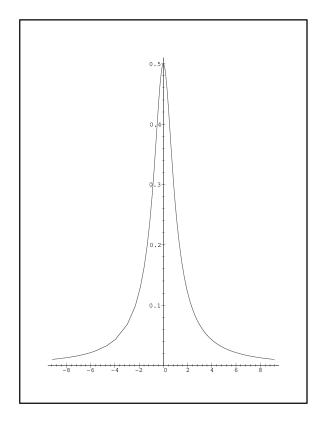
Figure 1: Conformal factor $A(\rho)$ is plotted as a function of $\rho$. $m\lambda$ is set to 1.

Our strategy is to expand the metric and equations of motion around the classical solution to the first order of the fluctuation. In the following investigation, we use the formalism developed in [21]. We parametrize the metric as $g_{\mu\rho}{(e^{h})^{\rho}}_{\nu}$ where $g_{\mu\nu}$ is the background metric and ${h^{\rho}}_{\rho}=0$ (traceless). The tensor indices are raised and lowered by the background metric. This formalism explicitly separates ${h^{\mu}}_{\nu}$ from the conformal mode of the metric.

The equation of the motion with respect to ${h^{\mu}}_{\nu}$ is

$${R^{\mu}}_{\nu}+2\nabla^{\mu}\nabla_{\nu}\phi-{1\over 2}{H_{3}^{\mu}}{H_{3\nu}}+\cdots=\kappa^{2}{T^{\mu}}_{\nu},$$ (2.12)

where $\kappa=e^{\phi}$. We have suppressed the contributions from the R-R sector. The advantage to consider the four dimensional traceless energy momentum tensor ${T^{\mu}}_{\nu}$ is that all other equations of motion are satisfied to the first order of ${h^{\mu}}_{\nu}$. In this sense it minimally excites gravitons.

Eq. (2.12) is expanded to the first order of ${h^{\mu}}_{\nu}$ as

$${1\over 2}\nabla^{\rho}\nabla_{\rho}{h^{\mu}}_{\nu}-{1\over 2}h^{\mu\rho},_{\rho\nu}-{1\over 2}h_{\nu\rho},^{\rho\mu}$$ (2.13)

$$-{h^{\mu}}_{\nu},^{\rho}\partial_{\rho}\phi-{1\over 2}{H^{\mu}}_{\rho\tau}{H_{\nu}}^{\sigma\tau}{h^{\rho}}_{\sigma}-{1\over 4}{H^{\rho}}_{\sigma\tau}{H_{\nu}}^{\sigma\tau}{h^{\mu}}_{\rho}+\cdots$$

$$= -\kappa^{2}{T^{\mu}}_{\nu}.$$

In the coordinate system of eq.(2.9), it is consistent to assume that the tensor indices of the nonvanishing ${h^{\alpha}}_{\beta}$ resides in the four dimensional space-time since the tensor indices of ${T^{\alpha}}_{\beta}$ are also four dimensional. It is also consistent to assume that ${h^{\alpha}}_{\alpha}=0$ since ${T^{\alpha}}_{\alpha}=0$. We also adopt the $h^{\alpha\gamma},_{\gamma}=0$ gauge.

Our strategy is to first study the following free equation of motion for ${{h}^{\alpha}}_{\beta}$ in the ten dimensional curved space-time:

$${1\over 2}\nabla^{\mu}\nabla_{\mu}{{h}^{\alpha}}_{\beta}=-\kappa^{2}{T^{\alpha}}_{\beta}.$$ (2.14)

Eq.(2.14) can be rewritten as:

$${H}{{h}^{\alpha}}_{\beta} = 2A\kappa^{2}{T^{\alpha}}_{\beta},$$

$${H} = -{A\over\sqrt{g}}\partial_{\mu}\sqrt{g}g^{\mu\nu}\partial_{\nu}.$$ (2.15)

The Hamiltonian is

$$H=-{1\over(m\lambda)^{1\over 2}}(\vec{\nabla}^{2}+{\partial^{2}\over\partial\rho^{2}}+{3\over 2}{A^{\prime}\over A}{\partial\over\partial\rho}+A\hat{L}^{2}),$$ (2.16)

where $A^{\prime}={\partial A/\partial\rho}$. The symbols $\vec{\nabla}^{2}$ and $\hat{L}^{2}$ denote the Laplacians on $R^{4}$ and $S^{5}$ respectively. We can further simplify eq. (2.15) by the similarity transformation as

$$\tilde{H}A^{{3\over 4}}h_{\alpha\beta} = 2\kappa^{2}A^{7\over 4}T_{\alpha\beta},$$

$$\tilde{H} = A^{3/4}HA^{-3/4}$$ (2.17)

$$= -{1\over(m\lambda)^{1\over 2}}(\vec{\nabla}^{2}+{\partial^{2}\over\partial\rho^{2}}-{3\over 4}{A^{\prime\prime}\over A}+{3\over 16}{A^{\prime 2}\over A^{2}}+A\hat{L}^{2}).$$

We concentrate on the $S$ wave on $S^{5}$ in what follows. The eigenfunction of $\tilde{H}$ is found to be $exp(i\vec{k}\cdot\vec{x})\tilde{\phi}_{l}$ with the eigenvalue ${(m\lambda)^{-1\over 2}}(\vec{k}^{2}+E_{l})$. Note that $E_{l}$ acts as the four dimensional mass of the various modes. It can be obtained by solving the following quantum mechanics problem

$$(-{\partial^{2}\over\partial\rho^{2}}+{3\over 4}{A^{\prime\prime}\over A}-{3\over 16}{A^{\prime 2}\over A^{2}})\tilde{\phi}=E\tilde{\phi}.$$ (2.18)

Let us introduce a super-charge

$$Q={\partial\over i\partial\rho}\sigma_{1}+{3\over 4}{A^{\prime}\over A}\sigma_{2}.$$ (2.19)

Since the relevant Hamiltonian can be embedded in $Q^{2}$, we only need to solve $Q\tilde{\phi}=0$ to find the zeromodes. The solution is

$$\tilde{\phi}=e^{{3\over 4}\int d\rho({A^{\prime}\over A})}.$$ (2.20)

We conclude that there is a single zero energy bound state with the conformal factor $A$ of our type as follows

$$\tilde{\phi}_{0}=A^{3\over 4}.$$ (2.21)

Such a zero mode corresponds to a massless field in four dimensions.

The propagator in this basis is

$$G(x,y)=\sum_{n}<x|n>{1\over E_{n}}<n|y>,$$ (2.22)

where $|n>$ is the eigenstate of $\tilde{H}$ with the eigenvalue $E_{n}$. We may adopt the vacuum saturation type approximation by only considering $<x|n>=exp(i\vec{k}\cdot\vec{x})\tilde{\phi}_{0}$ as the intermediate states. In this way we obtain the propagator of massless fields in four dimensions:

$$G(x,y) \sim \int d^{4}kexp(i\vec{k}\cdot(\vec{x}-\vec{y})){1\over{k}^{2}}\tilde{\phi}_{0}(\rho)\tilde{\phi}_{0}(\rho^{\prime})$$ (2.23)

$$\sim {1\over(\vec{x}-\vec{y})^{2}}\tilde{\phi}_{0}(\rho)\tilde{\phi}_{0}(\rho^{\prime}).$$

As the final result of these investigations, we find the following gravitational interaction:

$$-{1\over 2}\int d^{10}xA^{5\over 2}(\rho){T_{\mu}}^{\nu}(\vec{x},\rho){h^{\mu}}_{\nu}(\vec{x},\rho)$$ (2.24)

$$= -\int d^{10}x\int d^{10}yA^{7\over 4}(\rho){T_{\alpha}}^{\beta}(\vec{x},\rho)\tilde{\phi}_{0}(\rho){1\over(\vec{x}-\vec{y})^{2}}\tilde{\phi}_{0}(\rho^{\prime})\kappa^{2}(\rho^{\prime}){T^{\alpha}}_{\beta}(\vec{y},\rho^{\prime})A^{7\over 4}(\rho^{\prime})$$

$$\sim -\bar{\kappa}^{2}\int d^{4}x\int d^{4}y{\tilde{T}_{\alpha}}^{\beta}(\vec{x}){\tilde{T}^{\alpha}}_{\beta}(\vec{y}){1\over(\vec{x}-\vec{y})^{2}}.$$

We have introduced the four dimensional energy momentum tensor

$${\tilde{T}^{\alpha}}_{\beta}(\vec{x})=\int d\rho d\Omega_{5}{T^{\alpha}}_{\beta}(\vec{x},\rho)A^{5\over 2}(\rho).$$ (2.25)

The interaction between them is of the four dimensional graviton exchange type with the gravitational coupling $\tilde{\kappa}=\kappa(0)$.

Here we remark on the Hermiticity of the Hamiltonians in eqs. (2.16) and (2.18). The latter is Hermitian with respect to the trivial norm since

$$\int d\rho\tilde{\phi}({\partial\over i\partial\rho}-i{3\over 4}{A^{\prime}\over A})({\partial\over i\partial\rho}+i{3\over 4}{A^{\prime}\over A})\tilde{\phi}$$ (2.26)

$$= \int d\rho(-{\partial\over i\partial\rho}-i{3\over 4}{A^{\prime}\over A})\tilde{\phi}\ ({\partial\over i\partial\rho}+i{3\over 4}{A^{\prime}\over A})\tilde{\phi}.$$

It is translated into the Hermiticity condition on the former after the similarity transformation as

$$\int d\rho A^{3\over 2}(-{\partial\over i\partial\rho})\phi({\partial\over i\partial\rho})\phi\\ \sim\int d\rho\sqrt{g}g^{\rho\rho}{\partial\over\partial\rho}\phi{\partial\over\partial\rho}\phi,$$

where $\phi=A^{-3/4}\tilde{\phi}$. Therefore our Hamiltonian is positive definite with respect to the natural norm defined by the string frame metric $g_{\mu\nu}$. In this sense our important physical input is our identification of the physical metric with string frame metric $g_{\mu\nu}$. We have checked that our zero mode remains the exact zero mode after taking account of other terms in eq.(2.13).

Therefore we argue that we can obtain four dimensional gravity with $NCYM_{4}$ a la Randall-Sundrum[5]. Since not only the metric but also the dilaton expectation value (string coupling) rapidly decay in the large $r$ region, we expect that there is essentially nothing outside the noncommutativity scale transverse to the ‘brane’. In fact we have postulated this kind of ‘compactification’ mechanism in the matrix models [3][4][45]. We have expected that four dimensional gravitation is obtained if the eigenvalue distribution of the matrices are four dimensional. It is because the matrices represent space-time coordinates in our proposal. In our interpretation, there is simply nothing outside the support of the eigenvalue distributions, not even space-time.

We observe that this Euclidean solution can be analytically continued into Minkowski space-time only in the small $r$ region. One possible interpretation of such a solution is to maintain that Minkowski space-time appears from $NCYM_{4}$ as its low energy approximation. We may identify the noncommutativity scale with Planck scale if we apply this model to our space-time. Although the Lorentz invariance is broken at the noncommutativity scale in this model, such a possibility is not excluded by the experiments. Therefore $NCYM_{4}$ is a candidate of the unified theory of interactions. We explain in the subsequent sections that IIB matrix model naturally provides us with such a theory. We still need to solve many problems such as breaking SUSY and finding chiral fermions to construct a realistic unified theory. We hope that these problems can be solved by further investigations in IIB matrix model.

3 Noncommutative field theories as twisted reduced models

In this section we briefly recapitulate our formulation of NCYM through large $N$ reduced models. We have pointed out that well-known twisted reduced models[23][24] are equivalent to NCYM. This connection is further studied in[28][29][38]. We consider $d$ dimensional $U(n)$ gauge theory coupled to adjoint matter as an example:

$$S=-\int d^{d}x{1\over g^{2}}Tr({1\over 4}[D_{\mu},D_{\nu}][D_{\mu},D_{\nu}]+{1\over 2}\bar{\psi}\Gamma_{\mu}[D_{\mu},\psi]),$$ (3.1)

where $\psi$ is a Majorana spinor field. The corresponding reduced model is

$$S=-{1\over g^{2}}Tr({1\over 4}[A_{\mu},A_{\nu}][A_{\mu},A_{\nu}]+{1\over 2}\bar{\psi}\Gamma_{\mu}[A_{\mu},\psi]).$$ (3.2)

Now $A_{\mu}$ and $\psi$ are $n\times n$ Hermitian matrices and each component of $\psi$ is $d$-dimensional Majorana-spinor.

We expand $A_{\mu}=\hat{p}_{\mu}+\hat{a}_{\mu}$ around the following classical solution

$$[\hat{p}_{\mu},\hat{p}_{\nu}]=iB_{\mu\nu},$$ (3.3)

where $B_{\mu\nu}$ are $c$-numbers. We assume the rank of $B_{\mu\nu}$ to be $\tilde{d}$ and define its inverse $C^{\mu\nu}$ in $\tilde{d}$ dimensional subspace. The directions orthogonal to the subspace is called the transverse directions. $\hat{p}_{\mu}$ satisfy the canonical commutation relations and they span the $\tilde{d}$ dimensional phase space. The semiclassical correspondence shows that the volume of the phase space is $V_{p}=n(2\pi)^{\tilde{d}/2}\sqrt{detB}$.

We Fourier decompose $\hat{a}_{\mu}$ and $\hat{\psi}$ fields as

$$\hat{a} = \sum_{k}\tilde{a}(k)exp(iC^{\mu\nu}k_{\mu}\hat{p}_{\nu}),$$

$$\hat{\psi} = \sum_{k}\tilde{\psi}(k)exp(iC^{\mu\nu}k_{\mu}\hat{p}_{\nu}),$$ (3.4)

where $exp(iC^{\mu\nu}k_{\mu}\hat{p}_{\nu})$ is the eigenstate of adjoint $P_{\mu}=[\hat{p}_{\mu},~{}]$ with the eigenvalue $k_{\mu}$. The Hermiticity requires that $\tilde{a}^{*}(k)=\tilde{a}(-k)$ and $\tilde{\psi}^{*}(k)=\tilde{\psi}(-k)$.

We can construct a map from a matrix to a function as

$$\hat{a}\rightarrow a(x)=\sum_{k}\tilde{a}(k)exp(ik\cdot x),$$ (3.5)

where $k\cdot x=k_{\mu}x^{\mu}$. By this construction, we obtain the $\star$ product

$$\hat{a}\hat{b} \rightarrow a(x)\star b(x),$$

$$a(x)\star b(x) \equiv exp({C^{\mu\nu}\over 2i}{\partial^{2}\over\partial\xi^{\mu}\partial\eta^{\nu}})a(x+\xi)b(x+\eta)|_{\xi=\eta=0}.$$ (3.6)

The operation $Tr$ over matrices can be exactly mapped onto the integration over functions as

$$Tr[\hat{a}]=\sqrt{detB}({1\over 2\pi})^{\tilde{d}\over 2}\int d^{\tilde{d}}xa(x).$$ (3.7)

The twisted reduced model can be shown to be equivalent to NCYM by the the following map from matrices onto functions

$$\hat{a} \rightarrow a(x),$$

$$\hat{a}\hat{b} \rightarrow a(x)\star b(x),$$

$$Tr \rightarrow \sqrt{detB}({1\over 2\pi})^{\tilde{d}\over 2}\int d^{\tilde{d}}x.$$ (3.8)

The following commutator is mapped to the covariant derivative:

$$[\hat{p}_{\mu}+\hat{a}_{\mu},\hat{o}]\rightarrow{1\over i}\partial_{\mu}o(x)+a_{\mu}(x)\star o(x)-o(x)\star a_{\mu}(x)\equiv[D_{\mu},o(x)],$$ (3.9)

We may interpret the newly emerged coordinate space as the semiclassical limit of $\hat{x}^{\mu}=C^{\mu\nu}\hat{p}_{\nu}$. Therefore we can interpret $A_{\mu}$ as momenta as well in IIB matrix model with noncommutative backgrounds since $\hat{x}$ and $\hat{p}$ are linearly related. It is the reflection of the remarkable T-duality property of the theory. The space-time translation is realized by the following unitary operator:

$$exp(i\hat{p}\cdot d)\hat{x}^{\mu}exp(-i\hat{p}\cdot d)\\ =\hat{x}^{\mu}+d^{\mu}.$$

Applying the rule eq.(3.8), the bosonic action becomes

$$-{1\over 4g^{2}}Tr[A_{\mu},A_{\nu}][A_{\mu},A_{\nu}]$$ (3.10)

$$= {\tilde{d}nB^{2}\over 4g^{2}}-\sqrt{detB}({1\over 2\pi})^{\tilde{d}\over 2}\int d^{\tilde{d}}x{1\over g^{2}}({1\over 4}[D_{\alpha},D_{\beta}][D_{\alpha},D_{\beta}]$$

$$+{1\over 2}[D_{\alpha},\varphi_{\nu}][D_{\alpha},\varphi_{\nu}]+{1\over 4}[\varphi_{\nu},\varphi_{\rho}][\varphi_{\nu},\varphi_{\rho}])_{\star}.$$

In this expression, the indices $\alpha,\beta$ run over $\tilde{d}$ dimensional world volume directions and $\nu,\rho$ over the transverse directions. We have replaced $a_{\nu}\rightarrow\varphi_{\nu}$ in the transverse directions. Inside $(~{}~{})_{\star}$, the products should be understood as $\star$ products and hence commutators do not vanish. The fermionic action becomes

$${1\over g^{2}}Tr\bar{\psi}{\Gamma}_{\mu}[A_{\mu},\psi]$$ (3.11)

$$= \sqrt{detB}({1\over 2\pi})^{\tilde{d}\over 2}\int d^{\tilde{d}}x{1\over g^{2}}(\bar{\psi}{\Gamma}_{\alpha}[D_{\alpha},\psi]+\bar{\psi}\Gamma_{\nu}[\varphi_{\nu},\psi])_{\star}.$$

We therefore find noncommutative U(1) gauge theory. In order to obtain NCYM with $U(m)$ gauge group, we need to consider new classical solutions which are obtained by replacing each element of $\hat{p}_{\mu}$ by the $m\times m$ unit matrix:

$$\hat{p}_{\mu}\rightarrow\hat{p}_{\mu}\otimes{\mathbf{1}}_{m}.$$ (3.12)

The Hermitian models are invariant under the unitary transformation: $A_{\mu}\rightarrow UA_{\mu}U^{\dagger},\psi\rightarrow U\psi U^{\dagger}$. As we shall see, the gauge symmetry can be embedded in the $U(N)$ symmetry. We expand $U=exp(i\hat{\lambda})$ and parameterize

$$\hat{\lambda}=\sum_{k}\tilde{\lambda}(k)exp(i{k}\cdot\hat{x}).$$ (3.13)

Under the infinitesimal gauge transformation, we find the fluctuations around the fixed background transform as

$$\hat{a}_{\mu} \rightarrow \hat{a}_{\mu}+i[\hat{p}_{\mu},\hat{\lambda}]-i[\hat{a}_{\mu},\hat{\lambda}],$$

$$\hat{\psi} \rightarrow \hat{\psi}-i[\hat{\psi},\hat{\lambda}].$$ (3.14)

We can map these transformations onto the gauge transformation in NCYM by our rule eq.(3.8):

$$a_{\alpha}(x)\rightarrow a_{\alpha}(x)+{\partial\over\partial x^{\alpha}}\lambda(x)-ia_{\alpha}(x)\star\lambda(x)+i\lambda(x)\star a_{\alpha}(x),$$

$$\varphi_{\nu}(x)\rightarrow\varphi_{\nu}(x)-i\varphi_{\nu}(x)\star\lambda(x)+i\lambda(x)\star\varphi_{\nu}(x),$$

$$\psi(x)\rightarrow\psi(x)-i\psi(x)\star\lambda(x)+i\lambda(x)\star\psi(x).$$ (3.15)

We have introduced another representation of matrices[15]. For simplicity we consider the two dimensional case first:

$$[\hat{x},\hat{y}]=-iC.$$ (3.16)

This commutation relation is realized by the guiding center coordinates of the two dimensional system of electrons in magnetic field. We recall that we have $n$ quanta with $n$ dimensional matrices. Each quantum occupies the space-time volume of $2\pi C$. We may consider a square von Neumann lattice with the lattice spacing $l_{NC}$ where $l_{NC}^{2}=2\pi C$. This spacing $l_{NC}$ gives the noncommutative scale. Let us denote the most localized state centered at the origin by $|0\rangle$. It is annihilated by the operator $\hat{x}^{-}=\hat{x}-i\hat{y}$. We construct states localized around each lattice site by utilizing translation operators $|x_{i}\rangle=exp(-ix_{i}\cdot\hat{p})|0\rangle$. They are the coherent states on a von Neumann lattice ${\bf x}_{i}=l_{NC}(n_{i}{\bf e}^{x}+m_{i}{\bf e}^{y})$ where $n,m\in{\bf Z}.$ The generalizations to arbitrary even $\tilde{d}$ dimensions are straightforward.

We evaluate the following matrix elements

$$\rho_{ij}\equiv\langle x_{i}|x_{j}\rangle=exp({i\over 2}B_{\mu\nu}x_{i}^{\mu}x_{j}^{\nu})exp(-{(x_{i}-x_{j})^{2}\over 4C}).$$ (3.17)

Although $|x_{i}\rangle$ are non-orthogonal, $\langle x_{i}|x_{j}\rangle$ exponentially vanishes when $(x_{i}-x_{j})^{2}$ gets large. We also find

$$\langle x_{i}|exp(ik\cdot\hat{x})|x_{j}\rangle=exp(ik\cdot{(x_{i}+x_{j})\over 2}+{i\over 2}B_{\mu\nu}x_{i}^{\mu}x_{j}^{\nu})exp(-{(x_{i}-x_{j}-d)^{2}\over 4C}),$$ (3.18)

where $d^{\mu}=C^{\mu\nu}k_{\nu}$. This matrix element sharply peaks at $x_{i}-x_{j}=d$. It supports our interpretation that the eigenstate $exp(ik\cdot\hat{x})$ with $|k_{\mu}|>2\pi/l_{NC}$ can be interpreted as string like extended objects whose length is $|C^{\mu\nu}k_{\nu}|$. When $|k_{\mu}|<2\pi/l_{NC}$, on the other hand, this matrix becomes close to diagonal whose matrix elements go like

$$\langle x_{i}|exp(ik\cdot\hat{x})|x_{j}\rangle\sim exp(ik\cdot x_{i})\langle x_{i}|x_{j}\rangle.$$ (3.19)

It again supports our interpretation that $exp(ik\cdot\hat{x})$ correspond to the ordinary plane waves when $|k_{\mu}|<2\pi/l_{NC}$. They are represented by the matrices which are close to diagonal.

Figure 2: Noncommutative fields are represented as bi-local fields on the von Neumann lattice with the lattice spacing $l_{NC}$. Small momentum modes ($|k|<2\pi/l_{NC}$) represent ordinary (commutative) fields. Large momentum modes ($|k|>2\pi/l_{NC}$) represent bi-local ‘open strings’ which are highly nonlocal. Only a fraction of the full momentum ($|k^{c}|<2\pi/l_{NC}$) can be interpreted as the momentum associated with the center of mass motion of an ‘open string’ on the von Neumann lattice. In the figure, $\delta d^{\mu}=C^{\mu\nu}k^{c}_{\nu}$.

We may expand matrices $\hat{\phi}$ in the twisted reduced model by the following bi-local basis as follows:

$$\hat{\phi}=\sum_{i,j}\phi(x_{i},x_{j})|x_{i}\rangle\langle x_{j}|,$$ (3.20)

where the Hermiticity of $\hat{\phi}$ implies $\phi^{*}(x_{j},x_{i})=\phi(x_{i},x_{j})$. The matrices $\hat{\phi}$ represent $\hat{a_{\mu}}$ or $\hat{\psi}$ in the super Yang-Mills case but the setting here is more generally applied to an arbitrary noncommutative field theory. The bi-local basis spans the whole $n^{2}$ degrees of freedom of matrices.

Here we work out the translation rule between the momentum eigenstate representation $\hat{\phi}=\sum_{k}\tilde{\phi}(k)exp(ik\cdot\hat{x})$ and the bi-local field representation of eq.(3.20):

$$\tilde{\phi}(k) = {1\over n}Tr(exp(-ik\cdot\hat{x})\hat{\phi})={1\over n}\sum_{i,j}\langle x_{i}|exp(-ik\cdot\hat{x})|x_{j}\rangle\ \phi(x_{j},x_{i})$$

$$= {1\over n}\sum_{x_{c}}\phi(x_{c},d)exp(-ik\cdot x_{c}),$$

$$\phi(x_{c},d) = \sum_{x_{r}}exp({i\over 2}B_{\mu\nu}x_{r}^{\mu}x_{c}^{\nu})exp(-{(x_{r}-d)^{2}\over 4C})\phi(x_{j},x_{i}),$$ (3.21)

where $x_{c}=(x_{i}+x_{j})/2$ and $x_{r}=x_{i}-x_{j}$. From eq.(3.21), we observe that the slowly varying field with the momentum smaller than $2\pi/l_{NC}$ consists of the almost diagonal components. Hence close to diagonal components of the bi-local field are identified with the ordinary slowly varying field $\phi(x_{c})$. On the other hand, rapidly oscillating fields are mapped to the off-diagonal open string states. A large momentum in the $\nu$-th direction $|k_{\nu}|>2\pi/l_{NC}$ corresponds to a large distance in the $\mu$-th direction $|d^{\mu}|=|C^{\mu\nu}k_{\nu}|>l_{NC}$.

We can decompose $d$ as $d=d_{0}+\delta d$ where $d_{0}$ is a vector which connects two points on the von Neumann lattice and $|\delta d^{\mu}|<l_{NC}$. This decomposition is illustrated in Figure 2. Then the summation over $x_{r}$ in (3.21) is dominated at $x_{r}=d_{0}$. In this way the large momentum degrees of freedom are more naturally interpreted as extended open string-like fields. They are denoted by ‘open strings’ in this paper. In this representation, we make contact with the quenched reduced models [23] in the large momentum region.

Here we remark the important property concerning the infra-red and ultra-violet cut-offs of NCYM constructed with $n$ dimensional matrices. Since the unit lattice size of the von Neumann lattice is $l_{NC}$, the total lattice size is $l_{NC}n^{1/\tilde{d}}$. It implies that the maximum momentum is $2\pi n^{1/\tilde{d}}/l_{NC}$ by using the relation $\hat{p}_{\mu}=B_{\mu\nu}\hat{x}^{\nu}$. It in turn implies that the minimum momentum of the system is $2\pi/n^{1/\tilde{d}}l_{NC}$ since we have $n^{2}$ momentum modes. The matrix model construction of NCYM implies very natural infra-red and ultra-violet cut-offs which disappear in the large $n$ limit.

4 Estimations of the string scale

In this section, we estimate the string scale $\alpha^{\prime}_{eff}$ in IIB matrix model with noncommutative backgrounds. We have explained that the von Neumann lattice naturally appears in the preceding section. We argue that NCYM is superstring theory on the von Neumann lattice. We first give the arguments based on the tree level propagators. We then explain that our claim is supported by T-duality arguments. We give another evidence for it by investigating graviton exchange processes in the next section.

As we have shown in the preceding section, the momentum which can be associated with the center of mass motion of an ‘open string’ is not full $k_{\mu}$ but rather $k^{c}_{\mu}=B_{\mu\nu}\delta d^{\nu}$. There we have decomposed $d^{\mu}=C^{\mu\nu}k_{\nu}$ as $d=d_{0}+\delta d$ where $d_{0}$ is a vector which connects two points on the von Neumann lattice and $|\delta d^{\mu}|<l_{NC}$. We can indeed represent $\tilde{\phi}(k)$ of eq.(3.21) as follows:

$$\tilde{\phi}(k^{c},d)={1\over n}\sum_{x_{c}}\phi(x_{c},d)exp(-ik^{c}\cdot x_{c}).$$ (4.1)

It is because

$$exp(-iB_{\mu\nu}d_{0}^{\nu}x_{c}^{\mu})=1.$$ (4.2)

We interpret $\tilde{\phi}(k^{c},d)$ as the creation-annihilation operator for the open string with momentum $k^{c}$ and length $d$.

We consider the following tree level propagator:

$$\sum_{k_{0}}<\tilde{\phi}(-k)\tilde{\phi}(k)>exp(ik_{0}\tau)\sim exp(-m\tau)$$ (4.3)

where $k_{0}$ and $\vec{k}$ denote time-like and spatial momenta respectively in this section. The mass term is conventionally identified with the zero spacial momentum limit of the correlator eq.(4.3). In order to relate it to the mass of an ‘open string’, we consider a state with $k_{1}<2\pi/l_{NC}<k_{2},k_{3}$. Such a state is extended in $(x^{2},x^{3})$ plane with the length $l=C\sqrt{k_{2}^{2}+k_{3}^{2}}$. As we have argued, the momentum which can be associated with the center of mass motion of an ‘open string’ is not full $\vec{k}$ but rather $\vec{k}^{c}$. We find $m\sim Bl$ from the zero momentum limit ($\vec{k}^{c}\rightarrow 0$) of the correlator eq.(4.3). From these considerations, we propose to identify the mass of the state with the length $l>>l_{NC}$ as $Bl$. We recall that an open string with the length $l$ has the mass of $l/2\pi\alpha^{\prime}$. Therefore we find $2\pi\alpha^{\prime}_{eff}=C$ with such an identification.

We remark that our estimate is consistent with the string theory arguments. From eq.(2.7), we have indeed found that the $\alpha^{\prime}_{eff}\sim c$ in section 2. A hint for such an identification has been found in a finite temperature investigation in [33]. Our estimate is also consistent with the space-time uncertainty principle of Yoneya[35].

It is certainly true that we obtain NCYM in the low energy limit of string theory with $b_{\mu\nu}$ backgrounds. In such a limit, we retain only those degrees of freedom whose masses are smaller than the string scale. However in IIB matrix model with noncommutative backgrounds, we also find very high energy modes which may be interpreted as long ‘open strings’ due to the relation $\hat{x}^{\mu}=C^{\mu\nu}\hat{p}_{\nu}$. As can be seen in eq.(2.7) they are as massive as oscillator modes if their lengths exceed $l_{NC}$. We therefore emphasize here that our formulation is not a low energy limit of string theory. The graviton exchanges are observed only because we have very long ‘open strings’ in the matrix model. To put it differently, infrared singular behaviors are observed in noncommutative field theory only if we consider the ultra-violet cut-off which is much larger than the noncommutativity scale. It is the reason why closed strings do not decouple in such a formulation.

In our picture, we interpret the bi-local fields as the zero modes of open strings. We classify the zero modes as ‘momentum modes’ and ‘winding modes’ as follows. We recall the von Neumann lattice $|x_{i}>$ which is constructed by the generators of the translation operators $U_{\mu}=exp(-il_{NC}e_{\mu}\cdot\hat{p})$. We can ‘compactify’ the theory by imposing the following conditions for fluctuations

$$\hat{\phi}=U_{\mu}\hat{\phi}U^{\dagger}_{\mu}.$$ (4.4)

In this T-dual picture, the von Neumann lattice can be identified with the lattice spanned by the winding modes. We thus classify those modes as ‘winding modes’. We have explained that $k^{c}_{\mu}$ can be interpreted as momentum modes which can be associated with the center of mass motion of ‘open strings’ on the von Neumann lattice. We thus classify them as ‘momentum modes’.

In string theory, the introduction of constant $b_{\mu\nu}$ background is known to interpolate the Neumann and Dirichlet boundary conditions. In the large and small $b_{\mu\nu}$ limit, we find Dirichlet and Neumann boundary conditions respectively. We find only ‘winding’ and ‘momentum’ modes in these limits. If we expand IIB matrix model around the commutative backgrounds, we only find ‘winding’ modes. In string theory we also find only ‘winding’ modes if we consider strings which connect D instantons. The advantage of noncommutative backgrounds is that we find the both ‘momentum’ and ‘winding’ modes.

Since we have found the both ‘momentum’ and ‘winding’ modes, it is no surprise that the theory possesses T duality. The remarkable property of NCYM is the existence of Morita equivalent pairs [36][20][37]. We propose that two Morita equivalent theories can be related by the exchange of the ‘momentum’ and ‘winding’ modes.

We have argued that the ‘winding’ modes of NCYM span the von Neumann lattice whose lattice unit size is $l_{NC}$. The total lattice size is $l_{NC}n^{1/\tilde{d}}$. We may reinterpret it as the maximum momentum $2\pi n^{1/\tilde{d}}/l_{NC}$ of the dual lattice. The dual lattice possesses the unit lattice size of $l_{NC}/n^{1/\tilde{d}}$. We consider a twisted large $N$ reduced model on such a lattice. In this way we find a pair of theories with the compactification radii $R=l_{NC}n^{1/\tilde{d}}/2\pi$ and $R^{\prime}=l_{NC}/n^{1/\tilde{d}}2\pi$. They are related by the duality transformation $R^{\prime}=\alpha^{\prime}_{eff}/R$ with $2\pi\alpha^{\prime}_{eff}=C$. Next we recall that the ‘momentum’ modes of NCYM are quantized in the unit of $l_{NC}/n^{1/\tilde{d}}C$. We can naturally reinterpret them as the ‘winding’ modes of the dual lattice. These winding modes can be obtained by introducing the unit magnetic flux in $U(n)$ gauge theory by imposing twisted boundary conditions. In this sense NCYM and twisted reduced models are Morita equivalent [38].

We remark that the T-duality transformation we have discussed is expressed by the following open string metric transformation in string theory[20]

$$G_{\mu\nu}\rightarrow\Theta^{\mu\rho}G_{\rho\sigma}(\Theta^{T})^{\sigma\nu}$$ (4.5)

where $\Theta^{\mu\nu}=C^{\mu\nu}/(2\pi R^{2})\sim 1/n^{2/\tilde{d}}$. Our interpretation is that the two metrics which are related by the T-duality transformation in eq.(4.5) describe two tori we have just constructed. We conclude that our estimate of the inverse string tension $2\pi\alpha^{\prime}_{eff}=C$ is also supported by the T-duality arguments. We argue that this is the exact result since it is obtained from the exact T duality property of the theory.

5 Graviton exchange processes

In this section, we study gravitational interactions in IIB matrix model with noncommutative backgrounds. To be specific, we consider photon-photon scattering via exchange of a graviton. This process can be studied by considering block-block interactions. Namely we consider the backgrounds of the following type:

$$A_{\mu} = \left(\begin{array}[]{cc}p_{\mu}+a_{\mu}&0\\ 0&p_{\mu}+a^{\prime}_{\mu}\end{array}\right),$$ (5.3)

where $a_{\mu}$ and $a^{\prime}_{\mu}$ denote the backgrounds which represent two colliding photons.

The one-loop effective action of IIB matrix model is

$$ReW=\frac{1}{2}{\cal T}r\log(P_{\lambda}^{2}\delta_{\mu\nu}-2iF_{\mu\nu})-\frac{1}{4}{\cal T}r\log((P_{\lambda}^{2}+\frac{i}{2}F_{\mu\nu}\Gamma^{\mu\nu})(\frac{1+\Gamma_{11}}{2}))-{\cal T}r\log(P_{\lambda}^{2}).$$ (5.4)

Here $P_{\mu}$ and $F_{\mu\nu}$ are operators acting on the space of matrices as

$$P_{\mu}X = [p_{\mu},X],$$

$$F_{\mu\nu}X = \left[f_{\mu\nu},X\right],$$ (5.5)

where $f_{\mu\nu}=i[p_{\mu},p_{\nu}]$. Now we expand the general expression of the one-loop effective action (5.4) with respect to the inverse powers of the relative distance between the two blocks. We quote the general expression in what follows[1]:

$$W = -{\cal T}r\left(\frac{1}{P^{2}}F_{\mu\nu}\frac{1}{P^{2}}F_{\nu\lambda}\frac{1}{P^{2}}F_{\lambda\rho}\frac{1}{P^{2}}F_{\rho\mu}\right)$$ (5.6)

$$-2{\cal T}r\left(\frac{1}{P^{2}}F_{\mu\nu}\frac{1}{P^{2}}F_{\lambda\rho}\frac{1}{P^{2}}F_{\mu\rho}\frac{1}{P^{2}}F_{\lambda\nu}\right)$$

$$+\frac{1}{2}{\cal T}r\left(\frac{1}{P^{2}}F_{\mu\nu}\frac{1}{P^{2}}F_{\mu\nu}\frac{1}{P^{2}}F_{\lambda\rho}\frac{1}{P^{2}}F_{\lambda\rho}\right)$$

$$+\frac{1}{4}{\cal T}r\left(\frac{1}{P^{2}}F_{\mu\nu}\frac{1}{P^{2}}F_{\lambda\rho}\frac{1}{P^{2}}F_{\mu\nu}\frac{1}{P^{2}}F_{\lambda\rho}\right)+O((F_{\mu\nu})^{5}).$$

Since $P_{\mu}$ and $F_{\mu\nu}$ act on the $(i,j)$ blocks independently, the one-loop effective action $W$ is expressed as the sum of contributions of the $(i,j)$ blocks $W^{(i,j)}$. Therefore we may consider $W^{(i,j)}$ as the interaction between the $i$-th and $j$-th blocks.

Using (5.6) we can easily evaluate $W^{(i,j)}$ to the leading order of $1/\sqrt{(d^{(i)}-d^{(j)})^{2}}$ as

$$W^{(i,j)} = {1\over r^{8}}(-{\cal T}r^{(i,j)}(F_{\mu\nu}F_{\nu\lambda}F_{\lambda\rho}F_{\rho\mu})-2{\cal T}r^{(i,j)}(F_{\mu\nu}F_{\lambda\rho}F_{\mu\rho}F_{\lambda\nu})$$ (5.7)

$$+{1\over 2}{\cal T}r^{(i,j)}(F_{\mu\nu}F_{\mu\nu}F_{\lambda\rho}F_{\lambda\rho})+{1\over 4}{\cal T}r^{(i,j)}(F_{\mu\nu}F_{\lambda\rho}F_{\mu\nu}F_{\lambda\rho})$$

$$= {3\over 2r^{8}}(-n_{j}\tilde{b}_{8}(f^{(i)})-n_{i}\tilde{b}_{8}(f^{(j)})$$

$$-8Tr(f_{\mu\nu}^{(i)}f_{\nu\sigma}^{(i)})Tr(f_{\mu\rho}^{(j)}f_{\rho\sigma}^{(j)})+Tr(f_{\mu\nu}^{(i)}f_{\mu\nu}^{(i)})Tr(f_{\rho\sigma}^{(j)}f_{\rho\sigma}^{(j)})),$$

where

$$\tilde{b}_{8}(f)={2\over 3}(Tr(f_{\mu\nu}f_{\nu\lambda}f_{\lambda\rho}f_{\rho\mu})+2Tr(f_{\mu\nu}f_{\lambda\rho}f_{\mu\rho}f_{\lambda\nu})-{1\over 2}Tr(f_{\mu\nu}f_{\mu\nu}f_{\lambda\rho}f_{\lambda\rho})-{1\over 4}Tr(f_{\mu\nu}f_{\lambda\rho}f_{\mu\nu}f_{\lambda\rho})).$$ (5.8)

So the photon-photon scattering amplitude which corresponds to nonplanar diagrams in noncommutative gauge theory is

$${3\over 2r^{8}}(-8Tr(f_{\mu\nu}^{(i)}f_{\nu\sigma}^{(i)})Tr(f_{\mu\rho}^{(j)}f_{\rho\sigma}^{(j)})+Tr(f_{\mu\nu}^{(i)}f_{\mu\nu}^{(i)})Tr(f_{\rho\sigma}^{(j)}f_{\rho\sigma}^{(j)}))$$ (5.9)

$$= {3\over 2}({1\over 2\pi})^{\tilde{d}}B^{\tilde{d}-8}\int d^{\tilde{d}}x\int d^{\tilde{d}}y{1\over(x-y)^{8}}$$

$$\{-8tr(f_{\mu\nu}(x)f_{\nu\sigma}(x))tr(f_{\mu\rho}(y)f_{\rho\sigma}(y))+tr(f_{\mu\nu}(x)f^{\mu\nu}(x))tr(f_{\rho\sigma}(y)f^{\rho\sigma}(y))\},$$

where we have used our mapping rule eq. (3.8).

We consider the scattering of two incident photons with the wave functions

$$e(p)_{\mu}exp(ip\cdot x),~{}~{}e(q)_{\mu}exp(iq\cdot x),$$ (5.10)

where $p^{2}=q^{2}=0$ and $p\cdot e(p)=q\cdot e(q)=0$. In this case

$$f_{\mu\nu}(p) = p_{\mu}e(p)_{\nu}-p_{\nu}e(p)_{\mu},$$

$$f_{\mu\rho}(p)f^{\rho\nu}(-q) = -p_{\mu}q\cdot e(p)e(-q)_{\nu}-q_{\nu}p\cdot e(-q)e(p)_{\mu}$$ (5.11)

$$+p_{\mu}q_{\nu}e(p)\cdot e(-q)+e(p)_{\mu}e(-q)_{\nu}p\cdot q.$$

If we consider the forward scattering limit $k=p-q\rightarrow 0$:

$$f_{\mu\rho}(p)f^{\rho\nu}(-q)\rightarrow p_{\mu}p_{\nu},$$ (5.12)

we find only graviton exchange in this limit.

$$-{12}({1\over 2\pi})^{\tilde{d}}B^{\tilde{d}-8}\int d^{\tilde{d}}x\int d^{\tilde{d}}y{1\over(x-y)^{8}}tr(f_{\mu\rho}(x)f^{\rho\nu}(x))tr(f_{\mu\sigma}(y)f^{\sigma\nu}(y)).$$ (5.13)

This expression reminds us the one photon exchange amplitude between two conserved currents $j$ and $\tilde{j}$ in $QED_{4}$:

$$\int{d^{4}k\over(2\pi)^{4}}j_{\mu}(-k){1\over k^{2}+i\epsilon}\tilde{j}^{\mu}(k)$$ (5.14)

$$= {i\over 4\pi}\int d^{4}x\int d^{4}yj_{\mu}(x){1\over(x-y)^{2}-i\epsilon}\tilde{j}^{\mu}(y).$$

We decompose currents into positive and negative frequency parts

$$j_{\mu}(x) = j^{+}_{\mu}(x)+j^{-}_{\mu}(x),$$

$$j^{+}_{\mu}(x) = \int_{0}^{\infty}d\omega exp(-i\omega x^{0})j^{+}_{\mu}(\omega,\vec{x}),$$

$$j^{-}_{\mu}(x) = \int_{0}^{\infty}d\omega exp(i\omega x^{0})j^{-}_{\mu}(\omega,\vec{x}).$$ (5.15)

We rewrite eq.(5.14) as follows

$${1\over 4}\int d^{4}x\int d\vec{y}j^{-}_{\mu}(x^{0},\vec{x}){1\over|\vec{x}-\vec{y}|}\tilde{j}^{+\mu}(x^{0}-|\vec{x}-\vec{y}|,\vec{y})$$

$$+{1\over 4}\int d^{4}y\int d\vec{x}j^{+}_{\mu}(y^{0}-|\vec{x}-\vec{y}|,\vec{x}){1\over|\vec{x}-\vec{y}|}\tilde{j}^{-\mu}(y^{0},\vec{y}).$$ (5.16)

In this way we find retarded Lienard-Wiechert type interactions. The point we would like to make here is that covariance implies causality. Since ten dimensional covariance is manifest in IIB matrix model, it naturally leads to ten dimensional causality in Minkowski space-time. On the other hand, ensuring ten dimensional causality is highly nontrivial in $AdS$/CFT correspondence[39].

We recall the relevant part of the NCYM action as follows

$$B^{{\tilde{d}\over 2}-4}({1\over 2\pi})^{\tilde{d}\over 2}{1\over 4g^{2}}\int d^{\tilde{d}}xtr(f_{\alpha\beta}f^{\alpha\beta})_{\star}.$$ (5.17)

The energy momentum tensor can be read off from it in the low energy limit as

$$B^{{\tilde{d}\over 2}-4}({1\over 2\pi})^{\tilde{d}\over 2}{1\over g^{2}}(f_{\mu\rho}f^{\rho\nu}-{1\over 4}\delta_{\mu}^{\nu}f_{\rho\sigma}f^{\sigma\rho}).$$ (5.18)

So we can rewrite the gravitational interaction eq.(5.13) as follows

$$-{12}g^{4}\int d^{\tilde{d}}x\int d^{\tilde{d}}y{1\over(x-y)^{8}}T_{\mu\nu}(x)T^{\mu\nu}(y).$$ (5.19)

We recall the $\tilde{d}$ dimensional propagators

$$\int{d^{\tilde{d}}p\over(2\pi)^{\tilde{d}}}{1\over p^{2}}exp(ip\cdot x)={\Gamma({d-2\over 2})\over 4\pi^{\tilde{d}\over 2}}{1\over x^{\tilde{d}-2}}.$$ (5.20)

For $\tilde{d}=10$, we obtain

$$G_{10}(x)={3\over 2\pi^{5}}{1\over x^{8}}.$$ (5.21)

The gravitational coupling $\kappa$ is found to be

$$\kappa^{2}=16\pi^{5}g^{4}.$$ (5.22)

We also read off the $\tilde{d}$ dimensional Yang-Mills coupling from eq.(5.17) as

$$g^{2}_{YM}=C^{(\tilde{d}-8)/2}g^{2}(2\pi)^{\tilde{d}/2}.$$ (5.23)

Here we quote string theory predictions:

$$\kappa^{2}={1\over 2}(2\pi)^{7}g_{s}^{2}\alpha^{\prime 4},~{}~{}g^{2}_{YM}=(2\pi)^{\tilde{d}-3}g_{s}\alpha^{\prime(\tilde{d}-4)/2}.$$ (5.24)

Eq.(5.24) agrees with eq.(5.22) and eq.(5.23) with our identification $2\pi\alpha^{\prime}_{eff}=C$. We also find that the IIB matrix model coupling can be expressed by $\alpha^{\prime}_{eff}$ and $g_{s}$ as

$$g^{2}=(2\pi)g_{s}{\alpha^{\prime}_{eff}}^{2}.$$ (5.25)

which is consistent with our previous estimate through D-strings[1]. What these investigations indicate is that NCYM is superstring theory with the above identified string scale and string coupling. We have argued that it is superstring theory on the von Neumann lattice. Since the lattice spacing $l_{NC}$ is not visible in the low energy limit, it may be expected that it behaves like ordinary superstring theory in the low energy limit.

We find that the gravitational interaction eq.(5.19) exhibits the identical power law behavior $1/(x-y)^{8}$ irrespective of the dimensionality of the backgrounds $\tilde{d}$. It appears as if these background represent D-branes in flat ten dimensional space-time. However we argue that such an interpretation is premature since we have only considered the one loop effect here. We argue that a more reliable picture is obtained through supergravity approach which allows us to investigate nonperturbative effects.

As it is explained in section 2, we find Newton’s force law with these backgrounds. This is due to the existence of a massless bound state a la Randall and Sundrum. Such an effect is not visible in the perturbative calculations in this section. Therefore the supurgravity description of $NCYM_{4}$ suggests a nonperturbative compactification mechanism in IIB superstring and matrix model.

In the matrix model construction, the longitudinal size of the system is bounded by $l_{NC}n^{1/4}$. It also implies that the transversal size $r$ is bounded by $l_{NC}n^{1/4}$ since it is identified with the maximum energy scale of the system (multiplied by $l_{NC}^{2}$). In eq.(2.8), the dilaton expectation value is $O(1)$ at the noncommutativity scale $r^{2}\sim 1$. We then find $g_{\infty}$ is $O(1/n)$ since the dilaton decays like $1/r^{4}$ beyond the noncommutativity scale. We have fixed $\lambda=g_{\infty}\alpha^{\prime 2}b^{2}$ to be $O(1)$ which implies that $\alpha^{\prime}b\sim\sqrt{n}$. We conclude that $l_{NC}\sim l_{s}/n^{1/4}$ and $r$ never exceeds $O(l_{s})$ where $l_{s}$ is the string scale. Therefore there is simply no region with $r>l_{s}$ in the matrix model. We have taken the noncommutativity scale to be $O(1)$ and the cuff-off scale of $r$ becomes $O(n^{1/4})$. The cut-off can be removed in the large $n$ limit of the matrix model construction. In this way we can realize the entire space-time which is described by eq.(2.8).

6 Conclusions and Discussions

In this paper we have argued that we can obtain Newton’s force law with $NCYM_{4}$. Since it contains four dimensional gauge theory and gravitation, it is a candidate of the unified theory. It can be regarded as a compactification of ten dimensional IIB superstring straight down to four dimensions. It is naturally obtained in IIB matrix model with noncommutative backgrounds. Therefore it provides a nonperturbative compactification mechanism of matrix models.

We have identified the bi-local fields as the zero modes of open strings. They can be interpreted as the ‘momemtum’ and ‘winding’ modes on the von Neumann lattice. Our identification of the effective string scale with the noncommutativity scale is consistent with the exact T-duality which interchanges the ‘momentum’ and ‘winding’ modes. Although we have identified the zero modes of open strings, we have not constructed oscillator modes. We expect to find them in higher order diagrams. Let us consider a propagator (ribbon diagram). We associate it with a bi-local field since the double lines of the ribbon are mapped to two distinct space-time points. We need to draw many loops inside the ribbon at higher orders in perturbation theory. We can assign a space-time point to each loop. Our conjecture is that such an object can be interpreted as the propagator of oscillation modes. These arguments are illustrated in Figures 3 and 4.

It is important to recall here that we identify the string coupling with the topological expansion parameter of the Feynman diagrams of NCYM. It is not equal to the NCYM coupling although the both are related in the low energy limit as suggested by supergravity solutions. The tree level string propagator is obtained by summing all planar diagrams. Our proposal that NCYM with maximal SUSY may be interpreted as superstring theory on the von Neumann lattice should be understood in this context.

Figure 3: Propagators of bi-local fields. The two end-points are mapped onto space-time coordinates.

Figure 4: Higher order corrections to propagators of bi-local fields may render the bi-local fields stringy.

As we have pointed out, NCYM is obtained with a particular classical background in IIB matrix model. IIB matrix model is postulated as a nonperturbative formulation of superstring theory. In our proposal, the matrices $A_{\mu}$ are to be interpreted as space-time coordinates. If so, $\tilde{d}$ dimensional distributions of eigenvalues of matrices represent $\tilde{d}$ dimensional space-time. It is then expected that we find $\tilde{d}$ dimensional gauge theory and gravitation with such a background. In this paper we have argued that it is indeed the case with maximally supersymmetric backgrounds. From the findings in this paper, we draw the conclusion that NCYM provides a strong support for our basic premises of our IIB matrix model conjecture.

Acknowledgments

This work is supported in part by the Grant-in-Aid for Scientific Research from the Ministry of Education, Science and Culture of Japan.

References

- [1] N. Ishibashi, H. Kawai, Y. Kitazawa and A. Tsuchiya, A Large-N Reduced Model as Superstring, Nucl. Phys. B498 (1997) 467; hep-th/9612115.
-
[2]
J. Maldacena,
Adv. Theo. Math. Phys. 2 (1998), 231;hep-th/9711200
S.S. Gubser, I.R. Klebanov and A.M. Polyakov, Phys.Lett. B428 (1998), 105;hep-th/9802109.
E. Witten, Adv. Math. Phys. 2 (1998),253;hep-th/9802150. - [3] H. Aoki, S. Iso, H. Kawai, Y. Kitazawa and T. Tada, Space-Time Structures from IIB Matrix Model, Prog.Theor.Phys. 99 (1998)713; hep-th/9802085
- [4] H. Aoki, S. Iso, H. Kawai, Y. Kitazawa, A. Tsuchiya and T. Tada, IIB Matrix Model Prog. Theor. Phys. Suppl. 134 (1999) 47; hep-th/9908038.
- [5] L. Randall and R. Sundrum, An Alternative to Compactification; hep-th/9906064.
- [6] J. Polchinski, Phys. Rev. Lett. 75 (1995) 4724.
- [7] A. Connes, M. Douglas and A. Schwarz, JHEP 9802: 003.1998; hep-th/9711162.
- [8] H. Aoki, N. Ishibashi, S. Iso, H. Kawai, Y. Kitazawa and T. Tada, Noncommutative Yang-Mills in IIB matrix model, Nucl. Phys. 565 (2000) 176; hep-th/9908141.
- [9] A. Hashimoto and N. Itzhaki, Noncommutative Yang-Mills and the /CFT correspondence; hep-th/9907166.
- [10] J. Maldacena and J. G. Russo, Large N limit of noncommutative gauge theory; hep-th/9908134.
- [11] T. Banks, W. Fischler, S.H. Shenker and L. Susskind, Phys. Rev. D55 (1997) 5112; hep-th/9610043.
- [12] W. Taylor, Phys.Lett. B394 (1997) 283, hepth/9611042.
- [13] A. Connes, Comm. Math. Phys. 182 (1996) 155; hep-th/9603053.
- [14] N. Ishibashi, S. Iso, H. Kawai and Y. Kitazawa, Wilson loops in noncommutative Yang-Mills; hep-th/9910004, to appear in NPB.
- [15] S. Iso, H. Kawai and Y. Kitazawa, Bi-local Fields in Noncommutative Field Theory; hep-th/0001027, to appear in NPB.
- [16] Y. E. Cheung and M. Krogh, “Noncommutative geometry from 0-branes in a background B-field,” Nucl. Phys. B528 (1998) 185; hep-th/9803031.
- [17] F. Ardalan, H. Arfaei and M. M. Sheikh-Jabbari, “Noncommutative geometry from strings and branes,” JHEP 9902 (1999) 016; hep-th/9810072.
- [18] C. Chu and P. Ho, “Noncommutative open string and D-brane,” Nucl. Phys. B550 (1999) 151 [hep-th/9812219]; “Constrained quantization of open string in background B field and noncommutative D-brane,” Nucl. Phys. B568 (2000) 447 [hep-th/9906192].
- [19] V. Schomerus, JHEP 9906 (1999) 030; hep-th/9903205.
- [20] N. Seiberg and E. Witten, String theory and noncommutative geometry; hep-th/9908142.
- [21] H. Kawai, Y. Kitazawa and M. Ninomiya, Nucl PHys. B393 (1993) 280.
- [22] G. ’t Hooft and M. Veltman, Ann. Inst. Henri Poincare 20 (1974) 69.
-
[23]
T. Eguchi and H. Kawai, Phys. Rev. Lett. 48 (1982) 1063.
G. Parisi, Phys. Lett. 112B (1982) 463.
D. Gross and Y. Kitazawa, Nucl. Phys. B206 (1982) 440.
G. Bhanot, U. Heller and H. Neuberger, Phys. Lett. 113B (1982) 47.
S. Das and S. Wadia, Phys. Lett. 117B (1982) 228. - [24] A. Gonzalez-Arroyo and M. Okawa, Phys. Lett. B120 (1983) 174, Phys. Rev D27 (1983) 2397, see also [25].
-
[25]
T. Eguchi and R. Nakayama, Phys.Lett. B126 (1983) 89
T. Filk, Phys. Lett. B376 (1996) 53 - [26] D.B. Fairlie, P. Fletcher and C.Z. Zachos, J. Math. Phys. 31 (1990) 1088.
- [27] I. Bars, Phys. Lett. 245B(1990)35.
- [28] J. Ambjorn, Y.M. Makeenko, J. Nishimura and R.J. Szabo, Finite matrix models of noncommutative gauge theory; hep-th/9911041.
- [29] I. Bars and D. Minic, Noncommutative geometry on discrete periodic lattice and gauge theory; hep-th/9910091
- [30] I. Chepelev and R. Roiban Renormalization of quantum field theories on noncommutative , I. Scalars; hep-th/9911098
- [31] S. Minwalla, M.V. Raamsdonk and N. Seiberg, Noncommutative Perturbative Dynamics; hep-th/9912072
- [32] M. Hayakawa, Perturbative analysis on infrared aspects of noncommutative QED on ; hep-th/9912094, Perturbative analysis on infrared and ultraviolet aspects of noncommutative QED on ; hep-th/9912167
- [33] W. Fischler, E. Gorbatov, A. Kashani-Poor, S. Paban, P. Pouliot and J. Gomis, Evidence for winding states in noncommutative quantum field theory; hep-th/0002067.
- [34] M.V. Raamsdonk and N. Seiberg, Comments on Noncommutative Perturbative Dynamics; hep-th/0002186
- [35] T. Yoneya, Prog. Theor. Phys. 97 (1997) , 949; hep-th/9703078.
- [36] B. Pioline and A. Schwarz, Morita equivalence and T duality; hep-th/9908019.
- [37] A. Hashimoto and N. Itzhaki, On the hierarchy between non-commutative and ordinary supersymmetric Yang-Mills, hep-th/9911057.
- [38] J. Ambjorn, Y.M. Makeenko, J. Nishimura and R.J. Szabo, Nonperturbative Dynamics of Noncommutative Gauge Theory; hep-th/0002158.
- [39] D. Bak and S.J. Rey, Holographic View of Causality and Locality via Branes in /CFT Correspondence; hep-th/9902101.
- [40] O. Andreev and H. Dorn, Diagrams of noncommutative phi-three theory from string theory; hep-th/0003113
- [41] Y. Kiem and S. Lee, UV/IR mixing in noncommutative field theory via open string loops; hep-th/0003145
- [42] A. Bilal, C.S. Chu and R. Russo, String theory and noncommutative field theores at one loop; hep-th/0003180
- [43] J. Gomis, M. Kleban, T. Mehen, M.Rangamani and S. Shenker, Noncommutative gauge dynamics from string worldsheet; hep-th/0003215
- [44] H. Liu and J. Michelson, Stretched strings in noncummutative field theory; hep-th/0004013
- [45] J. Nishimura and G. Vernizzi, Spontaneous breakdown of Lorentz invariance in IIB matrix model; hep-th/0003223
- [46] A. Dhar, G. Mandal and S. Wadia, Mod. Phys. Lett. A7(1992)3129; hep-th/9207011.
- [47] S. Iso, D. Karabali and B. Sakita, Phys. Lett. B296 (1992) 143; hep-th/9209003.