Intersecting branes with an arbitrary excess angle

Abstract

We find all possible static embeddings of a 4-brane in any dimension-6 spacetime with 4-dimensional Poincaré symmetry and a negative cosmological constant, subject to orbifolding across the brane. Our new solutions allow intersecting branes at an angle determined by a new dynamical parameter. A collection of branes intersecting in one 3-brane allows an arbitrary excess angle that can be related to a vacuum density along the intersection. The 3-brane must be stabilized by additional fine-tuned interactions. We also note that localization of gravity is tied to the approximate fine tuning of the brane tensions.

I Introduction

In the seminal paper [1] gravity lives in five-dimensional anti de-Sitter ($AdS_{5}$) spacetime, infinite but strongly curved. Due to the presence of one graviton bound state, related to the finite proper size of “bulk” spacetime, gravity is effectively localized to a 4-dimensional “brane”. This mechanism however works only on codimension 1 branes but could be indirectly generalized [2] by placing $D-4$ codimension 1 branes intersecting in one 3-brane (our world). The brane tension of each of these 4-branes localizes gravity in the respective dimension. Models have been built and their cosmological consequences analyzed in [3].

This geometric setup has also been used to address the cosmological constant. Static embeddings of 3-branes in $AdS_{5}$ spacetimes were found [4] where the induced metric is dS, Minkowski or AdS; the curvature of the brane could be made much smaller than the brane tension. The same solution, now for a 4-brane in 6 dimensions, was rediscovered in conformally flat form in [5]. It was observed in this paper that it is possible to embed a static 4-brane, plane in conformal coordinates, at any angle $\phi$ determined by the brane tension, $\sin\phi=\sigma/\sigma_{c}$, where $\sigma_{c}$ is a critical value for the brane tension. A vanishing observed cosmological constant (i.e. flat induced metric) is produced when $\sigma=\sigma_{c}$. Cutting out wedges of the bulk $AdS_{5}$ with some angle $\phi$ and pasting together $n$ copies can accommodate an excess angle $n\phi-2\pi$. This must match the 3-brane vacuum energy in the intersection. The wedges are stabilized by imposing orbifold boundary conditions on each 4-brane. Whereas in the original Randall-Sundrum models [1, 6] the 3-brane tension is fine tuned to the bulk cosmological constant, here it must be fine tuned to match the excess angle, a function of the 4-brane tensions.

A similar setup with different bulk cosmological constants in each wedge is considered in [7], although without the introduction of an excess angle and correspondingly, without a 3-brane tension. It has been speculated in this reference that an additional parameter of the solution could resolve the one remaining fine tuning. What we need is a flat direction; then a new dynamical mechanism could stabilize the cosmological constant at zero value. Any additional vacuum energy would result in the readjustment of the brane angles and the additional parameter.

In this paper we find such an additional parameter. Using Gaussian normal coordinates (GNC) of a 4-brane, we write down all vacuum solutions in the bulk (with a negative cosmological constant), satisfying the Ansatz with signature $+++++-$

$$ds^{2}=dw^{2}+B(w,y)dy^{2}+A(w,y)\eta_{\mu\nu}dx^{\mu}dx^{\nu}.$$ (1)

The 4-brane is located at $w=0$. The stability of the brane with orbifold boundary conditions (i.e. $w\leftrightarrow-w$ identified while $y,x^{\mu}$ are fixed) comes down to the Israel conditions [8] on the extrinsic curvature, $K_{ab}=-\frac{\sigma}{2}h_{ab}$, where $\sigma$ is the 4-brane tension in appropriate units ($h_{ab}$ is the extrinsic curvature of the brane).

There is considerable freedom in transforming the coordinates, still within the Ansatz of Eq. (1). In addition, the same bulk metric is found starting with brane with different tensions, embedded at various angles. After eliminating all these ambiguities we are left with four different solutions (in each case the $y$ coordinate is chosen to render the induced metric conformally flat):

• A solution $A$ in which only a supercritical tension brane can be embedded, $\sigma>\sigma_{c}$, where the induced metric has two curvature singularities at finite $y\rightarrow\pm y_{*}$ (these are also at finite proper distance)

and three solutions where only $\sigma<\sigma_{c}$ branes can be embedded, namely

• A solution $B$ where the induced metric has a curvature singularity at finite proper and coordinate) distance $y\rightarrow-y_{*}$ and an $AdS$ horizon at $y\rightarrow y_{+}$.

• A solution $C$ with $AdS$ horizon at both $y\rightarrow\pm y_{+}$. The $w\rightarrow\infty$ limit is also asymptotically AdS.

• A solution $D$ where both the bulk and the induced metric are AdS. This is the solution found previously [4, 5, 7].

(We do not consider the fine tuned case, $\sigma=\sigma_{c}$.)

All these solutions are vacuum solutions with a negative cosmological constant in the bulk, i.e. solutions with constant scalar curvature. With the exception of $D$, however, they are not maximally symmetric. The induced metric is not even a vacuum solution. It is worth noting that the corresponding embedding of 3-branes in 5 dimensional spacetimes can be similarly found, but the new solutions have little value because the induced 3-brane metric does not resemble our world at all.

All our solutions have four-dimensional Poincaré invariance and can be trivially generalized to any maximally symmetric 4-dimensional metric replacing $\eta_{\mu\nu}$ in Eq. (1). Eventually the function $A(w,y)$ is the same in that case, only $B(w,y)$ is changed. The solutions have a complicated mathematical form and are expressed in an implicit form as solutions of algebraic equations involving special functions.

The usual picture of localization of gravity to a codimension one brane acquires some peculiar features when the brane tension differs from the fine tuned value. The warp factor that effectively compactifies the bulk decreases up to a distance ${\cal O}\left(\frac{\sigma}{\sigma_{c}-\sigma}\,l_{AdS}\right)$ in the extra dimension, but further away from the brane it starts to grow exponentially. The resulting “tail” of the graviton wave function eventually delocalizes brane gravity. This effect is absent for exact fine tuning and is also relevant for 3-branes embedded in a 5 dimensional bulk, e.g. for the models in [4, 5, 7]. Models in which the brane tensions are far from their critical value do not seem to have brane gravity at all. We discuss in what extent this can be considered a coordinate artifact in Sec. II B.

At any point along the brane, another brane can be inserted at an angle determined by its tension. In coordinates where the first brane has a conformally flat induced metric, the second brane is curved. The (covariant) angle between the branes is $\phi=\pi\pm 2\arcsin(\sigma/V)$. The quantity $V$ is independent of the tension of the second brane but changes as the intersection point is moved along the first brane ($\pm$ corresponds to two solutions and tells if $A$ increases or decreases as one moves away from the intersection along the brane). For example, close to the curvature singularity $V\rightarrow\infty$. Consequently, when several such wedges are sewn together in the same point, all branes will have the same parameter $V$. Now the induced metric on each brane is determined only by this $V$ (and the choice of the $\pm$ sign), so that the first and last branes can always be identified in order to build a manifold around the intersection. The orbifolding condition only requires, for global consistency, that every second brane around the intersection has the same tension (and $\pm$ sign).

The new parameter $V$ tells what part of the full 6-dimensional spacetime is cut away. Its emergence is due to the fact that the solution is not maximally symmetric. In the case of and $AdS_{6}$ solution, when the intersection point is shifted, the change in the metric can be compensated by a coordinate transformation, i.e. all points are physically equivalent. In our spacetime this is not so and $V$ parameterizes this difference. Because the angle of the wedges depends on $V$, so does the total excess angle. The topological requirement that a vacuum density produces an excess angle can be satisfied without fine tuning: the gravitational equations simply set the brane angles and the parameter $V$ to the consistent value.

When a brane tension is put on the 3-brane, another condition arises [9, 10] which has not been discussed in [5, 7]. A positive 3-brane tension tries to minimize the 4-volume, which corresponds to minimizing the value of $A(w,y)$ at the intersection. There is such a minimum only in case $C$. Now at the minimum the value of $V$ is zero, so we loose the additional freedom we had when we only needed to stabilize the 4-branes. For purposes of illustration we consider the following unusual but consistent geometry. We take two branes (to be identified), of finite length. At each end the two are joined and the covariant intersection angle is taken to be more than $2\pi$. Upon identifying the two branes we find an asymptotically $AdS_{6}$ spacetime which satisfies the gravitational equations except the minimizing of $A(w,y)$. Introducing some additional repulsive interaction between the two 3-branes, one can keep them several (6-dimensional) Plank lengths apart to ensure the cancellation of the 4-dimensional cosmological constant. This requires a fine tuning of the new coupling constants.

The paper is organized as follows. In Sec. II we describe all possible embeddings of a 4-brane with 4-dimensional Poincaré invariance and detail our observations on the localization of gravity to the brane. Sec. III shows how intersecting branes can be embedded and explains the emerging additional parameter. In Sec. IV we show that these joining branes can be sewn together in a global manifold and illustrate on a simple model why the additional interaction strengths need to be fine tuned.

II Static 4-branes in 6 dimensions

As explained in the introduction, we are looking for solutions to the six-dimensional Einstein equations:

$$\overline{G}_{ab}\equiv R_{ab}-\frac{R}{2}g_{ab}-g_{ab}=0.$$ (2)

These equations follow from the action with a number of branes included,

$$S[g]=\int_{bulk}(\Lambda_{6}-2M_{6}^{4}R[g])+\int_{4-brane(s)}\Lambda_{5},$$ (3)

while the units are so chosen that the bulk cosmological constant is set to $-1$:

$$\frac{\Lambda_{6}}{4M_{6}^{4}}\rightarrow-1.$$ (4)

We are looking at metrics that satisfy the Ansatz of Eq. (1) and the Israel conditions [8] at $w=0$,

$$K_{ab}=-\frac{\sigma}{2}h_{ab}.\mbox{\ \ \ \ with\ \ \ \ }\sigma=\frac{\Lambda_{5}}{8M_{6}^{3}}$$ (5)

These conditions ensure that keeping the $w\geq 0$ half plane and pasting back on another copy with $w\leftrightarrow-w$ identified can accommodate a 4-brane with tension $\sigma$. Note that the critical (“fine tuned”) value of the 4-brane tension is at $\sigma_{c}=\sqrt{\frac{2}{5}}$ in our notation.

A direct calculation shows that the Einstein equations in the bulk become

$$0 = \left(4\frac{A_{yy}}{A}+\frac{A_{y}^{2}}{A^{2}}-2\frac{A_{y}}{A}\frac{B_{y}}{B}\right)+\left(3\frac{A_{w}^{2}}{A^{2}}+2\frac{A_{w}}{A}\frac{B_{w}}{B}-2\right)B$$ (6)

$$0 = \left(6\frac{A_{yy}}{A}-3\frac{A_{y}}{A}\frac{B_{y}}{B}\right)+\left(6\frac{A_{ww}}{A}+3\frac{A_{w}}{A}\frac{B_{w}}{B}+2\frac{B_{ww}}{B}-\frac{B_{w}^{2}}{B^{2}}-4\right)B$$ (7)

$$0 = 3\frac{A_{y}^{2}}{A^{2}}-\left(2-\frac{A_{w}^{2}}{A^{2}}-4\frac{A_{ww}}{A}\right)B$$ (8)

$$0 = \frac{A_{y}A_{w}}{A^{2}}-2\frac{A_{yw}}{A}+\frac{A_{w}}{A}\frac{B_{w}}{B}$$ (9)

while the Israel conditions are satisfied at $w=0$,

$$\frac{A_{w}}{A}=-\sigma\mbox{\ \ \ \ and\ \ \ \ }\frac{B_{w}}{B}=-\sigma.$$ (10)

In the following we use the notation $A(w,y)=e^{a(w,y)}$. Observe from Eq. (8) that we either have $a_{y}=0$ and $2-5a_{w}^{2}-4a_{ww}=0$ simultaneously, or $a_{y}\neq 0$ and $2-5a_{w}^{2}-4a_{ww}>0$. By calculating the curvature tensor element of ${R_{wtt}}^{w}$ we observe that a necessary condition to have a maximally symmetric bulk solution is $2-5a_{w}^{2}-10a_{ww}\equiv 0$.

In order to solve these equations in the $a_{y}\neq 0$ case we first express $B$ from Eq. (8),

$$B=\frac{3a_{y}^{2}}{2-5a_{w}^{2}-4a_{ww}},$$ (11)

and substitute this back into Eq. (9). The result contains only $w$-derivatives and can be solved as an ordinary differential equation for $a_{w}$ along the $y=const$ lines, which by construction are the brane orthogonal geodesics with affine parameter $w$:

$$\partial_{w}\frac{\left(2-5a_{w}^{2}-10a_{ww}\right)^{2}}{\left(2-5a_{w}^{2}-4a_{ww}\right)^{5}}=0.$$ (12)

This is a first order differential equation on $a_{w}$ with boundary condition $a_{w}(w=0)=-\sigma$, so that once the $w$-independent function $c_{1}(y)={\left(2-5a_{w}^{2}-10a_{ww}\right)^{2}}/{\left(2-5a_{w}^{2}-4a_{ww}\right)^{5}}$ is specified it has one unique solution. It is not hard to see that Eq. (7) is a consequence of Eqs. (8,12). The boundary condition on $B_{w}$ trivially follows from Eq. (9). Now Eq. (6) relates the function $c_{1}(y)$ to $a_{0}(y)\equiv a(0,y)$. Substituting $B$ from Eq. (8) into Eq. (6) we find

$$0=\partial_{y}\left(A\sqrt[5]{2-5a_{w}^{2}-10a_{ww}}\right)\equiv\partial_{y}\left(\left[A\left(2-5a_{w}^{2}-4a_{ww}\right)\right]^{5}c_{1}(y)\right).$$ (13)

The term in the last parenthesis, $e^{5c_{0}}\equiv\left[A\left(2-5a_{w}^{2}-4a_{ww}\right)\right]^{5}c_{1}(y)$, is independent of $w$, as can be checked by showing that its $w$-derivative is proportional to Eq. (12). Then Eq. (6) is equivalent to $c_{0}=const$. We can calculate, with $\eta=sign\left(2-5a_{w}^{2}-10a_{ww}\right)=\pm 1$,

$$c_{1}(y)=\frac{\exp 5[c_{0}-a_{0}(y)]}{\left\{\frac{3}{5}(2-5\sigma^{2})+\frac{2}{5}\eta\exp\frac{5}{2}[c_{0}-a_{0}(y)]\right\}^{5}}.$$ (14)

We have found all stable embeddings of a 4-brane with tension $\sigma$ satisfying the Ansatz in terms of the arbitrary constant $c_{0}$, the sign $\eta$ and an arbitrary function $a_{0}(y)$. The latter specifies the factor $A$ in the induced metric on the brane.

The unique solution of Eq. (12) can be written in an implicit form as follows. First introduce the quantity $v(y,w)=\frac{3}{5}\frac{2-5a_{w}^{2}}{2-5a_{w}^{2}-4a_{ww}}$, which can be found from solving the fifth order equation $(2-5\tau^{2})^{3}\overline{c}_{1}(y)=v^{3}(v-1)^{2}$ in terms of $\tau\equiv a_{w}$ and $\overline{c}_{1}(y)\equiv\frac{4\times 27}{5^{5}}c_{1}(y)$; this is actually a rewriting of the definition of $c_{1}(y)$. Multiple solutions of this equation will lead to the different solutions mentioned in the introduction. Using the result we calculate the integral

$$w=\int_{-\sigma}^{a_{w}(w,y)}\frac{d\tau}{r(\tau,y)}\mbox{\ \ \ \ with\ \ \ \ }r(\tau,y)\equiv a_{ww}=\frac{3}{20}(2-5\tau^{2})\left(\frac{5}{3}-\frac{1}{v}\right),$$ (15)

which determines $a_{w}$ as a function of $w,y$. Integrating it, $a(w,y)=a_{0}(y)+\int_{0}^{w}a_{w}(w,y)dw\,$, provides us with the function $A(w,y)\equiv\exp{a(w,y)}$. The function $B(w,y)$ is then found from Eq. (8).

The various solutions we are finding contain a great deal of redundancy that can be absorbed into coordinate transformations. A redefinition of the scale of the $x^{\mu}$ coordinates, $x^{\mu}\rightarrow\lambda x^{\mu}$ changes only $A\rightarrow\lambda^{2}A$, $a_{0}\rightarrow a_{0}+2\log{\lambda}$, $c_{0}\rightarrow c_{0}+2\log{\lambda}$. This freedom can be used to set $c_{0}=0$.

The remaining freedom in arbitrarily choosing the function $a_{0}(y)$ locally corresponds to a coordinate transformation $y\rightarrow\overline{y}(y)$. This can be seen from the fact that as long as $a_{0}^{\prime}(y)\neq 0$, the unique choice $\overline{y}(y)=A(0,y)$ provides $\overline{A}(0,\overline{y})=\overline{y}$ and the solution has no more continuous parameters left.

Instead of the above choice of the $\overline{y}$ coordinate, however, we find it more instructive to use coordinates in which the induced metric is conformally flat, i.e. $A(0,y)=B(0,y)$. Such coordinates always exist and can be found from any solution by the coordinate transformation to $\overline{y}=\int^{y}\sqrt{B/A}\,dy$. Now expressing $a_{y}$ from Eq. (11) and using the definition of $c_{0}$ together with Eq. (14) we find (for w=0)

$$A_{y}=\pm\sqrt{\frac{2-5\sigma^{2}}{5}A^{3}+\frac{2}{15}\eta\,e^{\frac{5}{2}c_{0}}\sqrt{A}}.$$ (16)

Using the variable $u(y)=u_{0}/\sqrt{A(0,y)}$ with $u_{0}=-\eta\frac{exp{\frac{c_{0}}{2}}}{\sqrt[5]{\frac{3}{2}(2-5\sigma^{2})}}$ we write this in the form

$$\left(\frac{du}{dy}\right)^{2}=\left(\frac{2-5\sigma^{2}}{20}u_{0}^{2}\right)\left(1-u^{5}\right).$$ (17)

Note that, only on the brane, the variables $u$ and $v$ are related by $1-\frac{1}{v}=u^{5}$.

A Classification of the solutions

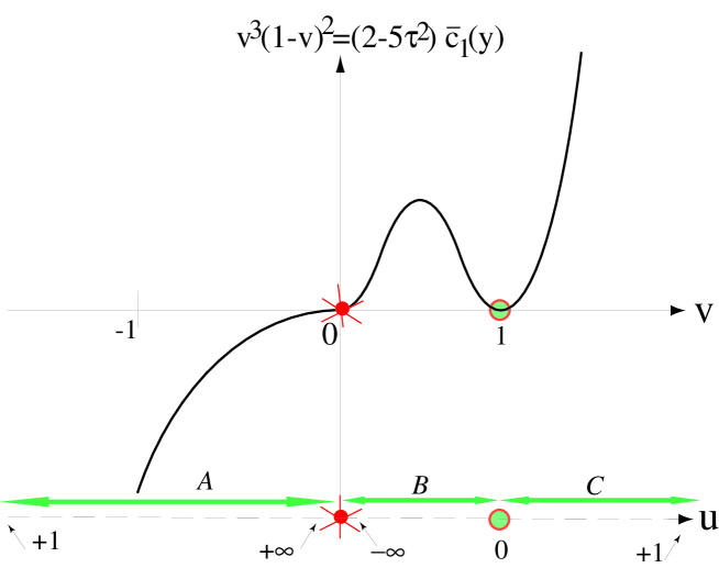
FIG. 1.: The algebraic equation whose solution determines the metric. The simultaneous change of the variable $u$, defined on the brane only, is shown, together with the various cases discussed in the text. $v=0$ is a curvature singularity and $v=1$ is an AdS horizon.

The various cases can be best understood by following the change of $v$ in Fig. 1 as we move along the brane. In the case $A$ when $\sigma^{2}>\frac{2}{5}$, only $u>1$, i.e. $v<0$ can satisfy Eq. (17). It has one solution, unique up to a translation of the $y$-coordinate,

$$u(y)=F_{s}\left[y\times u_{0}\sqrt{\frac{5\sigma^{2}-2}{20}}\right]\mbox{\ \ \ i.e.\ \ \ }A(0,y)=\frac{u_{0}^{2}}{F_{s}^{2}\left[y\times u_{0}\sqrt{\frac{5\sigma^{2}-2}{20}}\right]},$$ (18)

where the special function $F_{s}(\overline{y})$ is defined as the solution of $|\overline{y}|=\int_{0}^{F_{s}}\frac{du}{\sqrt{u^{5}-1}}$, see Fig. 2. The conformal factor of the induced metric, A(0,y) has a maximum at $y=0$ and vanishes at $y=\pm y_{*}=\pm\overline{y}_{*}u_{0}\sqrt{\frac{5\sigma^{2}-2}{20}}$. By direct calculation of the curvature of the induced metric one can establish the asymptotics, $R[g_{ab}^{(5)}]\propto\left(y_{*}\mp y\right)^{-\frac{10}{3}}$. The induced metric has curvature singularities at these points which are easily seen to be at finite proper distance.

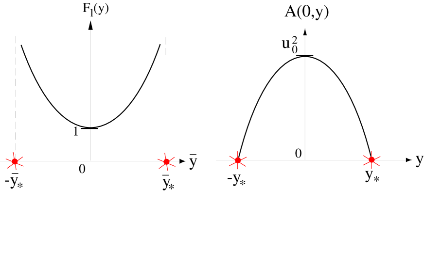
FIG. 2.: The special function $F_{s}(\overline{y})$ is defined for $-\overline{y}_{*}<\overline{y}<\overline{y}_{*}$, $\overline{y}_{*}\approx 0.911$. Also plotted is the conformal factor A(0,y) of the induced metric in case $A$, $ds^{2}=A(0,y)\left[dy^{2}+\eta_{\mu}\nu dx^{\mu}dx^{\nu}\right]$. The points $y=\pm y_{*}$ correspond to curvature singularities.

When $\sigma^{2}<\frac{2}{5}$ we must have $u<1$, i.e. $v>0$ to satisfy Eq. (17). Again, we the solution can be written in terms of a special function as

$$u(y)=F_{l}\left[y\times u_{0}\sqrt{\frac{2-5\sigma^{2}}{20}}\right]\mbox{\ \ \ i.e.\ \ \ }A(0,y)=\frac{u_{0}^{2}}{F_{l}^{2}\left[y\times u_{0}\sqrt{\frac{2-5\sigma^{2}}{20}}\right]},$$ (19)

where the special function $F_{l}(\overline{y})$ is now defined as the solution of $|\overline{y}|=\int_{F_{l}}^{1}\frac{du}{\sqrt{1-u^{5}}}$, plotted in Fig. 3. In the two equivalent regions where $F_{l}<0$, case $B$, $u$ is negative and $0<v<1$. The conformal factor of the induced metric $A(0,y)$ tends to zero at a curvature singularity at $y\rightarrow-y_{*}$, located at finite proper distance, and the scalar curvature diverges as $R[g_{ab}^{(5)}]\propto\left(y-y_{*}\right)^{-5}$. The function $A(0,y)$ increases with $y$ and at $y\rightarrow-y_{\odot}$ diverges. The asymptotics is $A(0,y)\approx\frac{20}{2-5\sigma^{2}}\frac{1}{(y+y_{\odot})^{2}}$, corresponding to an asymptotically $AdS_{5}$ induced metric. Consequently, the point $y=y_{\odot}$ is at infinite proper distance away, and the regions $B$ and $C$ should be understood as different solutions. In the region $-y_{\odot}<y<y_{\odot}$, case $C$, the conformal factor has a minimum and at the edges it diverges. The solution in this region sees $AdS$ horizons in both directions.

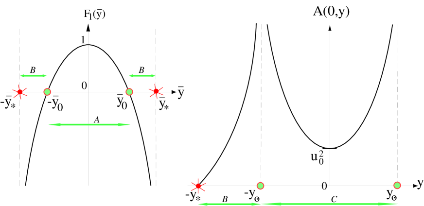
FIG. 3.: The special function $F_{l}(\overline{y})$ is defined for $-\overline{y}_{*}<\overline{y}<\overline{y}_{*}$, $\overline{y}_{*}\approx 2.804$. It is analytic at $\overline{y}=0$. Also plotted is the conformal factor of the induced metric in cases $B,C$. The points $y=\pm y_{*}$ correspond to curvature singularities, while $y=\pm y_{\odot}\,(\overline{y}_{\odot}\approx 1.254)$ are infinitely far away and represent $AdS$ horizons. The two regions with negative $F_{l}$ are related by a $y\rightarrow-y$ coordinate transformation.

The definition of $c_{0}$ according to Eq. (13) supposes that the solution is not maximally symmetric, $2-5a_{w}^{2}-10a_{ww}\neq 0$. If it is, corresponding to $c_{0}\rightarrow-\infty$, we have a fourth type of solution [4, 5]. This case $D$ corresponds to $v(w,y)\equiv 1$ as one can see from the relation $\frac{1}{v}-1=\frac{2}{3}\frac{2-5a_{w}^{2}-10a_{ww}}{2-5a_{w}^{2}}\rightarrow 0$. In terms of Fig. 1, the solution is “sitting” in the $AdS$ point. In our coordinates its form is

$$ds^{2}=dw^{2}+\frac{2-5\sigma^{2}}{2}\cosh^{2}\left[\frac{w}{\sqrt{10}}+\mbox{arctanh}\left(\sqrt{\frac{5}{2}}\sigma\right)\right]\times\left\{dy^{2}+\eta_{\mu\nu}dx^{\mu}dx^{\nu}e^{y\sqrt{\frac{2-5\sigma^{2}}{5}}}\right\}.$$ (20)

The induced metric on the brane is obviously $AdS_{5}$, as it should be.

The solutions we were finding for fixed values of $\sigma$ represent 6-dimensional spacetimes with an embedded 4-brane. They have no parameters (other than $\sigma$) that could not be absorbed into coordinate redefinitions. We will see in the next section, that different values of $\sigma$ actually correspond to embedding branes with different tensions in the same bulk metric and there are only three solutions altogether, corresponding to the cases $A,B,C$ above. No 4-branes can be embedded (within the confines of the metric Ansatz of Eq. (1)) in any other 6-dimensional spacetime.

In the exceptional case when $A(0,y)=const.$ along the brane it is not hard to see that there is no solution to our equations.

B A note on localization of gravity to the brane

In the brane GNC’s we are using, the large-$w$ asymptotic behavior of the functions $A$ and $B$ can be better understood in the form

$$A(w,y)\propto B(w,y)=\left(\frac{1-\sqrt{\frac{5}{2}}\sigma}{2}\right)^{2}e^{\sqrt{\frac{2}{5}}\,w}+\frac{1}{2}\left(1-\frac{5}{2}\sigma^{2}\right)+\left(\frac{1+\sqrt{\frac{5}{2}}\sigma}{2}\right)^{2}e^{-\sqrt{\frac{2}{5}}\,w}.$$ (21)

Far from the brane the first term dominates and evidently deconfines gravity. The form of the metric in the Randall-Sundrum model [1] is

$$ds^{2}=dw^{2}-\eta_{\mu\nu}dx^{\mu}dx^{\nu}e^{-2kw},$$ (22)

and the quick fall-off of the “warp factor” $e^{-2kw}$ is essential in localizing gravity to the brane (at least in the limit where the Kaluza-Klein excited modes can be neglected). What is happening?

The resolution of the paradox hinges on two points. First, observe that a change in $\sigma$ corresponds to a shift in $w$, in addition to rescaling $y$ and $x^{\mu}$, so that a brane with a different tension could be placed parallel to the original one in the same bulk. The RS brane corresponds to $\sigma^{2}\rightarrow\frac{2}{5}$, i.e. it is infinitely far away in $w$. The $\sigma\rightarrow\sigma_{c}$ limit is not smooth. Now consider a brane with tension just smaller than the fine tuned value, $\sigma_{c}-\sigma\ll\sigma_{c}$. The behavior of the functions $A,B$ for increasing $w$ is first governed by the second term, the warp factor falls off and there is brane-localized gravity. By the time the exponential compensates for the smallness of its coefficient and the first two terms start to dominate, the warp factor is already ${\cal O}\left(\frac{1-\sigma/\sigma_{c}}{2}\right)\ll 1$. It will grow again exponentially.

Second, the argument in [1] that leads to localization involves a Kaluza-Klein reduction, i.e. dropping the brane-orthogonal components of the metric (such as $g_{ww},g_{w\mu}$), in addition to the Kaluza-Klein expansion of the brane-tangential modes (i.e. $g_{\mu\nu}$). While close to the brane the separation of modes into brane-orthogonal and brane-tangential makes sense, far away it has no covariant meaning. The actual separation and large-$w$ behavior depends on the details of the model that explains the Kaluza-Klein reduction and cannot be expected to be faithfully represented by the general framework of [1]. One may conjecture by the same token that the increase in the warp factor is unphysical and should be thrown away.

In any case the conclusion remains that in any scenario where the brane tensions are not close to their fine tuned values does not automatically provide localized gravity. In order to make a coordinate invariant statement one needs to restrict to such coordinates in which the thrown-away modes ($g_{ww},g_{w\mu}$) are massive. It cannot be decided without the explicit identification of these modes whether the warp factor along the resulting $y=const$ lines shows the same behavior as Eq. (21). This is equally relevant for codimension one branes in five dimensions.

In this respect our most interesting solution, $C$, which has no curvature singularities, can be seen to have the asymptotic behavior

$$A(w,y)\approx function(y)\times e^{\sqrt{\frac{2}{5}}|w|}\left(1+2\frac{1+\sqrt{\frac{5}{2}}\sigma}{1-\sqrt{\frac{5}{2}}\sigma}e^{-\sqrt{\frac{2}{5}}|w|}+{\cal O}\left(e^{-\sqrt{\frac{2}{5}}|w|}\right)^{2}\right),$$ (23)

the same as the asymptotics of the known $AdS$ solutions.

III Intersecting branes

In the previous section we found all possible embeddings in GNC of the 4-brane. This still does not answer the question whether another brane can be inserted in the same bulk because for intersecting branes the two GNC’s certainly do not coïncide. In the CNC of one brane the other will not in general be straight. We were not able to solve the equations for the branes in closed form, but we could (almost) show their existence/unicity, and determine the relationship between the angle of intersection and the brane tensions.

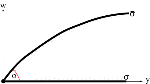
FIG. 4.: Cutting off a wedge with angle $\phi$. The vertical lines are the geodesics orthogonal to the $\sigma$ brane.

We start with one solutions which permits a 4-brane with tension $\sigma$ located at $w=0$, keeping the $W>0$ half brane. If effect we are considering a half-brane at $y\geq y_{0}$, and looking for another half-brane with tension $\tilde{\sigma}$, starting off at some angle $0<\phi<+\infty$, and keeping a wedge between them as shown in Fig. 4 (the wedge metric will of course be $2\pi$-periodic if $\phi>2\pi$.)

The condition for the stability of the $\tilde{\sigma}$ brane is again the Israel condition $K_{ab}=+\frac{\tilde{\sigma}}{2}h_{ab}$, where the opposite sign is due to the fact that this time we are keeping the bulk to the opposite side of the brane. We describe the brane with a pair of functions

$$\tilde{w}(\lambda),\tilde{y}(\lambda)\mbox{\ \ \ with\ \ \ }\tilde{w}(0)=0,\tilde{y}(0)=y_{0}\mbox{\ \ \ and\ \ \ }0\leq\lambda<\infty.$$ (24)

The Israel conditions become

$$2\left(\ddot{\tilde{y}}\dot{\tilde{w}}-\ddot{\tilde{w}}\dot{\tilde{y}}\right)+b_{y}\,\dot{\tilde{w}}\dot{\tilde{y}}^{2}+b_{w}\,\dot{\tilde{w}}\dot{\tilde{y}}\,\left(2\dot{\tilde{w}}+B\dot{\tilde{y}}\right) = \frac{\tilde{\sigma}}{\sqrt{B}}$$ (25)

$$\frac{a_{y}}{\sqrt{B}}\,\dot{\tilde{w}}-a_{w}\sqrt{B}\,\dot{\tilde{y}} = -\tilde{\sigma}$$ (26)

with $B=e^{b}$, where we fixed the $\lambda$ variable by requiring

$${\dot{\tilde{w}}}^{2}+B{\dot{\tilde{y}}}^{2}=1.$$ (27)

Now Eq. (26) can be viewed as a first order differential equation for the function $\tilde{w}(\tilde{y})$ with initial conditions set by $\tilde{w}(y_{0})=0$ and by Eq. (27). Up to a discreet ambiguity, this system has a unique solution. We could not show in complete generality that Eq. (25) is a consequence of Eq. (26), we expanded the solution of Eq. (26) in a power series around $\lambda=0$ keeping terms up to ${\cal O}(\lambda^{5})$ and saw that they did indeed satisfy Eq. (25), up to ${\cal O}(\lambda^{3})$. (The loss of two powers of $\lambda$ is due to the three derivatives figuring in Eq. (25).) We take this as an indication that Eq. (25) is indeed not an independent equation.

We can define the angle between the in a covariant way by requiring $\cos\phi=n_{a}g^{ab}\tilde{n}_{b}$, where $n_{a}$ and $\tilde{n}_{b}$ are the unit normals of the branes at the intersection. In our coordinates we find $\left(\sin\phi|\cos\phi\right)=\left(\dot{\tilde{w}}\left|\sqrt{B}\dot{\tilde{y}}\right.\right)_{\lambda=0}.$ Then, substituting this definition into Eq. (26) we see that the brane tension and the position of the junction (i.e. $y_{0}$) determines the angle:

$$\frac{a_{y}}{\sqrt{B}}\sin\phi+\sigma\cos\phi+\tilde{\sigma}=0.$$ (28)

A trivial check of this calculation is that $\phi=\pi$, $\tilde{\sigma}=\sigma$ is always a solution: the brane can always be continued across the point $y_{0}=0$. We also see that once Eq. (28) is satisfied, there is one unique solution to Eqs. (25-27).

Before discussing the solutions to Eq. 28 we look at the induced metric on the $\tilde{\sigma}$ brane. A simple substitution shows $d\tilde{s}^{2}=d\lambda^{2}+A\eta_{\mu\nu}dx^{\mu}dx^{\nu}$, which can be written in a conformally flat from by introducing the new variable $Y=\int_{0}^{\lambda}\frac{d\lambda}{\sqrt{A}}$ along the new brane: $d\tilde{s}^{2}=A\left(dY^{2}+\eta_{\mu\nu}dx^{\mu}dx^{\nu}\right)$. Note that the $x^{\mu}$ coordinates did not have to be rescaled, and the conformal factor A is the same at the junction in the two induced metrics. The bulk metric can now be written in GNC’s of the $\tilde{\sigma}$ brane in the form $ds^{2}=dW^{2}+\tilde{B}(W,Y)dY^{2}+\tilde{A}(W,Y)\eta_{\mu\nu}dx^{\mu}dx^{\nu}$; we know $\tilde{A}(0,Y)=\tilde{B}(0,Y)=A(\tilde{w},\tilde{y})$. But this must be one of our previously found solutions which comes with its $\tilde{v}(W,Y)$ function. A direct calculation of $\tilde{v}(0,0)$ gives, using Eq. (28), and observing $v=\frac{2-5\sigma^{2}}{5}\,\frac{\tilde{B}}{\tilde{a}_{Y}^{2}}$

$$\tilde{V}\equiv\tilde{\sigma}^{2}+\frac{2-5\tilde{\sigma}^{2}}{5\,\tilde{v}(0,0)}\ \ =\ \ V\equiv\sigma^{2}+\frac{2-5\sigma^{2}}{5\,v(0,0)}.$$ (29)

In other words, the quantity $V$ must be the same on the two sides of the wedge.

It will prove important to note now that once $\tilde{\sigma},\tilde{v}(0,0)$ and $\tilde{A}(0,0)$ are specified as they are, there are only two possible induced metrics on the new brane. The ambiguity results of the two ways to invert the functions $F_{l,r}$ and can be resolved by also specifying the sign $\tilde{\kappa}=\mbox{sign}\,{\tilde{a}_{Y}(0,0)}=\pm 1$. Then we will be able to argue that any two induced metrics with the same $\sigma,v(0,0),A(0,0)$ and $\kappa$ coïncide. This will be the situation when a number of wedges is pasted together around one 3-brane.

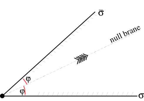
FIG. 5.: Cutting out a wedge between two branes with tensions $\sigma$ and $\tilde{\sigma}$. The double arrow shows the direction in A increases.

The solutions of Eq. (28) can be visualized by the following auxiliary device. It is always possible to find a unique solution $\phi=-\varphi$ to Eq. (28) with $\tilde{\sigma}=0$, also requiring $\tilde{\kappa}=+1.$ This corresponds to a “null brane” represented in Fig. 5. It is not hard to see that we could have started with the null brane and looked for the angles at which the two $\sigma,\tilde{\sigma}$ branes to cut out the wedge. The equations for their angles become

$$\frac{a_{y}}{\sqrt{B}}\sin\tilde{\varphi}+\tilde{\sigma}=0\mbox{\ \ \ and\ \ \ }\frac{a_{y}}{\sqrt{B}}\sin\varphi+\sigma=0,$$ (30)

where $\frac{a_{y}}{\sqrt{B}}=\sqrt{V}$ now refers to the null brane. The solutions that give the correct sign for the $a_{y}$’s are, with $-\frac{\pi}{2}\leq\arcsin\leq\frac{\pi}{2}$,

$$\varphi=\pi\frac{1-\kappa}{2}-\kappa\arcsin\frac{\sigma}{\sqrt{V}}+2\pi N\mbox{\ \ \ and\ \ \ }\tilde{\varphi}=\pi\frac{1-\tilde{\kappa}}{2}-\tilde{\kappa}\arcsin\frac{\tilde{\sigma}}{\sqrt{V}}+2\pi\tilde{N}.$$ (31)

Based on the “compatibility” of different branes, the possible setups can be classified as follows. It is not possible to move along any brane from one category to another.

• $0<V<\frac{2}{5}$, only branes with below critical tension, $\sigma^{2}<\frac{2}{5}$ can be used, all type $C$ (i.e. $v>1$) with no curvature singularity. The angles are determined by the tensions and the parameter $V$ which is fixed in any one junction but varies from junction to junction

• $V=\frac{2}{5}$, the spacetime is $AdS_{6}$, only type $D$ branes with below critical tension, $\sigma^{2}<\frac{2}{5}$ can be used. The angles are determined by the tensions and there is no additional parameter.

• $V>\frac{2}{5}$, one can accommodate both type $B$ branes with $0<\sigma^{2}<\frac{2}{5}$ and type $A$ branes with $\sigma^{2}>\frac{2}{5}$. There is again a parameter $V$ in the junctions. All induced metrics contain curvature singularities.

IV Sawing together the wedges

Any combination of intersecting branes with angles between them set according to Eq. (31) represents a stationary point of the action in Eq. (3). The $V$ are parameters of the solution, one at each intersection. We must make sure, however, that a globally defined metric exists when the pieces we have discussed are sewn together.

Each brane carries orbifold boundary conditions, which are easiest to state in GNC’s: we identify points with the sign of the corresponding coordinate $w$ flipped. This allows at most two different sets of 4-brane tensions ($\sigma$) in each intersection: every second one most be equal. The corresponding signs $\kappa$ should also be chosen equal. In we join an odd number of branes in one intersection, then all must have the same $\sigma$ and $\kappa$.

When $n=1,2,\dots$ branes intersect along one 3-brane, the $n+1^{th}$ one must be identified with the first one. There are two conditions that must be met for consistency. (i) The induced metric on the 3-brane must be the same for all wedges. This condition is always satisfied because the functions $A(0,0)$ are always the same and no rescaling of the $x^{\mu}$ coordinates was necessary. (ii) The induced metric on the $n+1^{th}$ brane must be identical with the induced metric on the $1^{st}$. This condition is again automatically satisfied because, as we saw, the equality of $V,A,\kappa$ and $\sigma$ is sufficient for that.

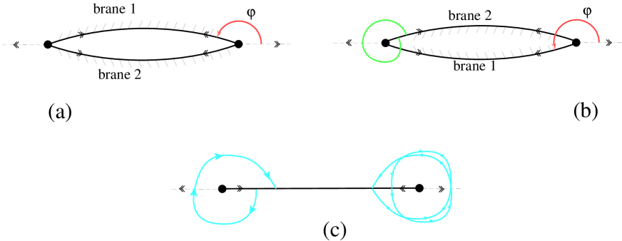
FIG. 6.: The illustrative geometry of the brane strip. In (a), the angles are distorted so that in actuality $\varphi>180^{0}$, while in (b) the angles are correct but the bulk is shown partially overlapping. The spirals show the part of the bulk that is retained. Finally, the two branes are identified as in (c). The double arrows show the direction in which $A$ increases. In (c) some of the brane orthogonal geodesics are shown (these represent the $y=const.$ lines in brane CNC).

In the following we consider a case with one positive tension 4-brane with two junctions around which the brane is identified with its own reverse side, shown in Fig. 6. We require, due to the effectively two dimensional gravity on the $w,y$ plane, an excess angle $0<\lambda<\pi$. This is possible only with $\kappa=-1$; and in order to have no curvature singularities, we will use type $C$ branes. Because then $a_{0}(y)$ must increase towards both “junctions”, it must have a minimum (at $y=0$) on the brane between then. Using the excess angles $\lambda_{1,2}$ as parameters, Eq. (31) tells the parameter (on each end separately) $V=\frac{\sigma^{2}}{\sin^{2}\frac{\lambda}{2}}$. Because for the $C$ type branes $V<\frac{2}{5}$, we can accommodate only an excess angle at least as large as $\sin\frac{\lambda}{2}>\sqrt{\frac{5}{2}}\sigma$. The 3-brane tension cannot be much smaller than the 4-brane tension. In brane GNC’s the conformal factor is $A(0,y)=F_{l}^{-2}\left[y\sqrt{\frac{2-5\sigma^{2}}{20}}\right]$, shown in Fig. 7. We calculated the position of the two ends of the brane, with the result

$$y_{j}=\frac{(-1)^{j}}{\sqrt{\frac{2-5\sigma^{2}}{20}}}\int_{u_{j}}^{1}\frac{du}{\sqrt{1-u^{5}}}\mbox{\ \ \ with\ \ \ }j=1,2.$$ (32)

The proper distance of the endpoints from the origin is

$$l_{j}=\frac{(-1)^{j}}{\sqrt{\frac{2-5\sigma^{2}}{20}}}\int_{u_{j}}^{1}\frac{du}{u\sqrt{1-u^{5}}}\mbox{\ \ \ with\ \ \ }u_{j}=\left[\frac{2\sin^{2}\frac{\lambda_{j}}{2}-5\sigma^{2}}{(2-5\sigma^{2})\sin^{2}\frac{\lambda_{j}}{2}}\right]^{\frac{1}{5}}.$$ (33)

Consistency requires that this distance should be $l\gg 1$ (otherwise the underlying field theory description of gravity is not justified). This requires that the 4-brane tension not be much smaller than $\lambda$ and also either $2-5\sigma^{2}\ll 1$ or $0<\sin\frac{\lambda}{2}-\sqrt{\frac{5}{2}}\sigma\ll 1$.

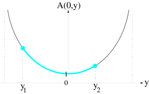
FIG. 7.: The conformal factor along the brane strip.

The presence of a vacuum energy density on the 3-brane requires the proper amount of excess angle. When this relationship is not satisfied, our Ansatz does not give a solution: the induced metric on the 3-brane is not flat any more. It is a trivial exercise to derive the equations of motion when a maximally symmetric but not flat 4-dimensional metric is allowed, i.e. $-dt^{2}+d{\bf x}^{2}$ is replaced by $-dt^{2}+d{\bf x}^{2}e^{2ht}$ in Eq. (1). We find that Eqs. (9,12) are not modified, so that the function $A(w,y)$ is not modified. The modification occurs because Eq. (11) gets replaced by

$$B=\frac{3a_{y}^{2}}{2-5a_{w}^{2}-4a_{ww}+12\frac{h^{2}}{A}},$$ (34)

so that $B(w,y)$ changes. This change also affects the intersection angles,

$$\frac{\tan^{2}\varphi_{h}}{\tan^{2}\varphi}=\frac{V}{V+4\frac{h^{2}}{A}}.$$ (35)

If the “mistuning” is little, $\delta\lambda=\lambda_{h}-\lambda=2(\phi_{h}-\phi)\ll 1$, the result is a small $h^{2}=-\frac{AV}{2\sin\lambda}\delta\lambda$. This translates to a small observable Hubble constant (the induced metric must be brought to the form $ds_{4}^{2}=-dt^{\prime 2}+d{\bf x}^{\prime 2}e^{2Ht^{\prime}}$, $H=h/\sqrt{A}$),

$$H^{2}=-\frac{\sigma^{2}}{\sin^{2}\frac{\lambda}{2}}\times\frac{\delta\lambda}{2\sin\lambda}.$$ (36)

Given that $\lambda$ cannot be made much smaller than $\sigma$, any sizable “mistuning” of $\lambda$ would result in a Hubble constant on the 6-dimensional Planck scale.

Up to this point however, we have not required any fine tuning. The 4-dimensional vacuum density, through the topologically required conical singularity of the metric enforces the adjustment of the parameter $V$ to its required value. However, when a 3-brane tension is added to the action,

$$S[g]=\int_{bulk}(\Lambda_{6}-2M_{6}^{4}R[g])+\int_{4-brane(s)}\Lambda_{5}+\int_{3-brane}\Lambda_{4},$$ (37)

the added term can be written as

$$\int_{3-brane}\Lambda_{4}=\Lambda_{4}\ A^{2}(0,0)\,\int_{3-brane}d^{4}x.$$ (38)

In order to avoid that the spacetime collapses onto the point where $A(0,0)$ is minimum, i.e. $y=0$, additional repulsive interactions have to be introduced. Their strength has to be fine tuned to ensure that the equilibrium length of the 4-brane is that of Eq. (33).

V Conclusions

The main result of this paper is that there exists embeddings of 4-branes in less than maximally symmetric 6-dimensional spacetimes that preserve 4-dimensional Poincaré invariance. Then different points on the 4-brane are not physically equivalent as they were in the $AdS$ case. The angle between intersecting branes, in any fixed intersection point, is always determined by the nondynamical parameters through the Israel conditions $K_{ab}=-\frac{\sigma}{2}h_{ab}$. We saw that there is no obstacle to building a global metric around the intersection and the additional parameter can be translated to an arbitrary excess angle. We also saw that there is no solution (without fine tuning the 4-brane tensions) with constant warp factor along the 4-brane. As a consequence, as we illustrated on a simple example, a 3-brane with tension tries to “move” to the mininum of that warp factor and additional interactions are needed to stabilize the 3-brane. We note that in all suggested solutions to the cosmological constant problem [10, 11, 12] in brane contexts some sort of tuning of the bulk interactions has been required.

VI Acknowledgments

The author thanks Bob Holdom for many useful discussions and stressing the importance of finding flat directions, as well as Hael Collins for discussions.

REFERENCES

- [1] L. Randall and R. Sundrum, “An alternative to compactification,” Phys. Rev. Lett. 83 (1999) 4690 [hep-th/9906064].
- [2] N. Arkani-Hamed, S. Dimopoulos, G. Dvali and N. Kaloper, “Infinitely large new dimensions,” Phys. Rev. Lett. 84, 586 (2000) [hep-th/9907209].
- [3] N. Arkani-Hamed, S. Dimopoulos, G. Dvali and N. Kaloper, “Manyfold universe,” hep-ph/9911386; S. Nam, “Mass gap in the Kaluza-Klein spectrum in a network of branewords,” [hep-th/9911237]; N. Kaloper, “Crystal manyfold universes in AdS space,” Phys. Lett. B474, 269 (2000) [hep-th/9912125]; J. Cline, C. Grojean and G. Servant, “Inflating intersecting branes and remarks on the hierarchy problem,” Phys. Lett. B472, 302 (2000) [hep-ph/9909496].
- [4] N. Kaloper, “Bent domain walls as braneworlds,” Phys. Rev. D60, 123506 (1999) [hep-th/9905210].
- [5] A. E. Nelson, “A new angle on intersecting branes in infinite extra dimensions,” hep-th/9909001.
- [6] L. Randall and R. Sundrum, “A large mass hierarchy from a small extra dimension,” Phys. Rev. Lett. 83, 3370 (1999) [hep-ph/9905221].
- [7] Cs. Csáki and Yu. Shirman, “Brane junctions in the Randall-Sundrum scenario,” Phys. Rev. D61, 024008 (2000) [hep-th/9908186].
- [8] W. Israel, “Singular Hypersurfaces And Thin Shells In General Relativity,” Nuovo Cim. B44 S10, 1 (1966).
- [9] A. Chodos and E. Poppitz, “Warp factors and extended sources in two transverse dimensions,” Phys. Lett. B471, 119 (1999) [hep-th/9909199].
- [10] J. Chen, M. A. Luty and E. Pontón, “A critical cosmological constant from millimeter extra dimensions,” hep-th/0003067.
- [11] N. Arkani-Hamed, S. Dimopoulos, N. Kaloper and R. Sundrum, “A small cosmological constant from a large extra dimension,” hep-th/0001197.
- [12] S. Kachru, M. Schulz and E. Silverstein, “Self-tuning flat domain walls in 5d gravity and string theory,” hep-th/0001206.