Abstract

We extend the recent computation of the tachyon potential by Berkovits, Sen and Zwiebach by including level two fields and keeping up to level four terms in the action. We find 90.5% of the expected result.

1 Introduction

During the last few years, it has been realized [1, 2, 3, 4] that Type IIA (IIB) string theory contains non-BPS D-branes of odd (even) spatial dimensions. An analysis of the open string states living on such a brane reveals the existence of a tachyon which comes from the NS sector. It has been argued by Sen [5, 6] that the tachyon potential has a minimum and that the minimum corresponds to the usual vacuum of closed string theory without any D-brane. This implies that the negative energy density contribution from the tachyon potential must exactly cancel the tension of the non-BPS D-brane.

To analyze the tachyon potential in order to test this conjecture, ordinary first quantized string theory cannot be used since the zero momentum tachyon state is not on-shell. We need an off-shell formalism of string theory. Such a formalism is given by string field theory. Recently it has been realized that calculating the tachyon potential in string field theory by including fields and terms in the string field action up to a certain level gives a good approximation to the tachyon potential. In [7, 8], the zeroth order and the first non-trivial correction to the tachyon potential on a non-BPS D-brane of Type II string theory was computed using open string field theory action formulated in [9, 10]. It was found that the potential has a minimum which cancels 60% of the D-brane tension at the zeroth level and 85% of the D-brane tension at the next non-trivial level (level 3/2). In this paper, we extend the work of [8] to include fields up to level 2. Similar computation was done in [13].

This paper is organized as follows: In section 2, we review the formalism of [7, 8] to set up the calculation. In section 3, we write down the expansion of the string field including fields up to level 2. We also give some details of the calculation — we give one simple example of calculation of a term in the action at each level. In the appendix, we list the conformal and BRST transformations of operators that we need in the calculation.

2 Superstring field theory on a Non-BPS D-brane

Superstring field theory on a non-BPS D-brane was described in detail in [8]. Here, we will just review the basic features to set up the calculation and establish notation. We will first review the essential features of string field theory on a BPS D-brane which only has a GSO(+) sector and then introduce Chan Paton matrices and GSO($-$) sector to discuss the non-BPS D-brane. We follow the notation and conventions of [8] throughout the paper.

BPS D-brane

In [9, 10, 7], a string field configuration in the GSO$(+)$ NS sector corresponds to a Grassmann even open string vertex operator $\Phi$ of ghost and picture number 0 [11] in the combined conformal field theory of a $c=15$ superconformal matter system, and the $b,c,\beta,\gamma$ ghost system with $c=-15$. Here, $b$, $c$ are the reparameterization ghosts and $\beta$, $\gamma$ are their superconformal partners. The $\beta$, $\gamma$ ghost system can be bosonized and can be replaced by ghost fields $\xi,\eta,\phi$, related to $\beta,\gamma$ through the relations

$$\beta=\partial\xi e^{-\phi},\qquad\gamma=\eta e^{\phi}.$$

The ghost number ($n_{g}$) and picture number ($n_{p}$) assignments and the conformal weights ($h$) are as follows [8]:

$$b:\quad n_{g}=-1,n_{p}=0,h=2\qquad c:\quad n_{g}=1,n_{p}=0,h=-1\,,$$

$$e^{q\phi}:\quad n_{g}=0,n_{p}=q,h=-(q+\frac{q^{2}}{2})\,,$$

$$\xi:\quad n_{g}=-1,n_{p}=1,h=0,\qquad\eta:\quad n_{g}=1,n_{p}=-1,h=1\,.$$

The SL(2,R) invariant vacuum has zero ghost and picture number.

We shall denote by $\langle\prod_{i}A_{i}\rangle$ the correlation function of a set of vertex operators in the combined matter-ghost conformal field theory on the unit disk with open string vertex operators inserted on the boundary of the disk, without including trace over CP factors. These correlation functions are to be computed with the normalization

$$\langle\xi(z)c\partial c\partial^{2}c(w)e^{-2\phi(y)}\rangle=2\,.$$ (1)

The BRST operator is given by

$$Q_{B}=Q_{0}+Q_{1}+Q_{2},$$

where

$$Q_{0} = =\oint dzc\bigl{(}T_{m}+T_{\xi\eta}+T_{\phi})+c\partial cb,$$

$$Q_{1} = \oint dz\eta\,e^{\phi}\,G_{m},\,\,\,\,\ Q_{2}=-\oint dz\eta\partial\eta e^{2\phi}b\,.$$ (2)

Here

$$T_{\xi\eta}=\partial\xi\,\eta,\quad T_{\phi}=-\textstyle\frac{1}{2}\partial\phi\partial\phi-\partial^{2}\phi\,,$$

$T_{m}$ is the matter stress tensor and $G_{m}$ is the matter superconformal generator. $G_{m}$ is a dimension $3/2$ primary field and satisfies:

$$G_{m}(z)G_{m}(w)\simeq{10\over(z-w)^{3}}+{2T_{m}\over(z-w)}\,.$$

The normalization of $\phi$, $\xi$, $\eta$, $b$ and $c$ are as follows:

$$\xi(z)\eta(w)\simeq{1\over z-w},\quad b(z)c(w)\simeq{1\over z-w},\quad\partial\phi(z)\partial\phi(w)\simeq-{1\over(z-w)^{2}}\,.$$

We denote by $\eta_{0}=\oint dz\eta(z)$ the zero mode of the field $\eta$ acting on the Hilbert space of matter ghost CFT.

The string field theory action is given by[7]

$$S={1\over 2g^{2}}\Bigl{\langle}\Bigl{\langle}(e^{-\Phi}Q_{B}e^{\Phi})(e^{-\Phi}\eta_{0}e^{\Phi})-\int_{0}^{1}dt(e^{-t\Phi}\partial_{t}e^{t\Phi})\{(e^{-t\Phi}Q_{B}e^{t\Phi}),(e^{-t\Phi}\eta_{0}e^{t\Phi})\}\Bigr{\rangle}\Bigr{\rangle}\,.$$ (3)

This action is defined by expanding all exponentials in a formal Taylor series. $\langle\langle A_{1},\ldots A_{n}\rangle\rangle$ is defined as:

$$\langle\langle A_{1}\ldots A_{n}\rangle\rangle=\Bigl{\langle}f^{(n)}_{1}\circ A_{1}(0)\cdots f^{(n)}_{n}\circ A_{n}(0)\Bigr{\rangle}\,.$$ (4)

Here, $f\circ A$ for any function $f(z)$, denotes the conformal transform of $A$ by $f$, and

$$f^{(n)}_{k}(z)=e^{2\pi i(k-1)\over n}\Big{(}{1+iz\over 1-iz}\Big{)}^{2/n}\,\quad\hbox{for}\quad n\geq 1.$$ (5)

In particular if $\varphi$ denotes a primary field of weight $h$, then

$$f\circ\varphi(0)=(f^{\prime}(0))^{h}\varphi(f(0))\,.$$

Since we have, in general, non-integer weight vertex operators, we should be more careful in defining $f\circ A$ for such vertex operators. Noting that

$$f^{(N)\prime}_{k}(0)={4i\over N}e^{2\pi i{k-1\over N}}\equiv{4\over N}e^{2\pi i({k-1\over N}+{1\over 4})}\,,$$

we adopt the following definition of $f^{(N)}_{k}\circ\varphi(0)$ for a primary vertex operator $\varphi(x)$ of conformal weight $h$:

$$f^{(N)}_{k}\circ\varphi(0)=\bigg{|}\Big{(}{4\over N}\Big{)}^{h}\bigg{|}e^{2\pi ih({k-1\over N}+{1\over 4})}\varphi(f^{(N)}_{k}(0))\,.$$ (6)

We also recall identities [8] which will be used in the calculation later:

$$\{Q_{B},\eta_{0}\}=0,\quad Q_{B}^{2}=\eta_{0}^{2}=0,$$

$$Q_{B}(\Phi_{1}\Phi_{2})=(Q_{B}\Phi_{1})\Phi_{2}+\Phi_{1}(Q_{B}\Phi_{2}),\quad\eta_{0}(\Phi_{1}\Phi_{2})=(\eta_{0}\Phi_{1})\Phi_{2}+\Phi_{1}(\eta_{0}\Phi_{2}),$$ (7)

$$\langle\langle Q_{B}(...)\rangle\rangle=\langle\langle\eta_{0}(...)\rangle\rangle=0.$$

Note that in the identities of the second line there are no minus signs necessary as $Q_{B}$ or $\eta_{0}$ go through the string field because the string field is Grassmann even (since we are in the GSO($+$) sector only).

Non-BPS D-brane

The algebraic structure described in the previous section works for the GSO($+$) (Grassman even) sector living on a BPS D-brane. However, on a non-BPS D-brane, the open string states live in both the GSO($-$) and GSO($+$) sector. The GSO($-$) states are Grassman odd and to incorporate them in the algebraic structure of the previous section, internal $2\times 2$ Chan Paton matrices were introduced in [8]. These are added both to the vertex operators and $Q_{B}$ and $\eta_{0}$ as described in detail below.

The $2\times 2$ identity matrix $I$ is attached on the usual GSO$(+)$ sector and the Pauli matrix $\sigma_{1}$ to the GSO$(-)$ sector. The complete string field is thus written as

$${\widehat{\Phi}}=\Phi_{+}\otimes I+\Phi_{-}\otimes\sigma_{1}\,,$$

where the subscripts denote the $(-)^{F}$ eigenvalue of the vertex operator. In addition, $Q_{B}$ and $\eta_{0}$ are tensored with $\sigma_{3}$:

$$\widehat{Q}_{B}=Q_{B}\otimes\sigma_{3},\qquad\widehat{\eta}_{0}=\eta_{0}\otimes\sigma_{3}\,.$$

We define

$$\langle\langle\widehat{A}_{1}\ldots\widehat{A}_{n}\rangle\rangle={\rm Tr\ }\Bigl{\langle}f^{(n)}_{1}\circ{\widehat{A}}_{1}(0)\cdots f^{(n)}_{n}\circ{\widehat{A}}_{n}(0)\Bigr{\rangle}\,,$$ (8)

where the trace is over the internal Chan Paton matrices. As in [8], fields or operators with internal CP matrices included are denoted by symbols with a hat on them, and fields or operators without internal CP matrices included are denoted by symbols without a hat.

In addition, we have the analogs of (7) holding:

$$\{{\widehat{Q}_{B}},{\widehat{\eta}_{0}}\}=0,\quad{\widehat{Q}_{B}}^{2}={\widehat{\eta}_{0}}^{2}=0,$$

$${\widehat{Q}_{B}}(\widehat{\Phi}_{1}\widehat{\Phi}_{2})=({\widehat{Q}_{B}}\widehat{\Phi}_{1})\widehat{\Phi}_{2}+\widehat{\Phi}_{1}({\widehat{Q}_{B}}\widehat{\Phi}_{2}),\quad{\widehat{\eta}_{0}}(\widehat{\Phi}_{1}\widehat{\Phi}_{2})=({\widehat{\eta}_{0}}\widehat{\Phi}_{1})\widehat{\Phi}_{2}+\widehat{\Phi}_{1}({\widehat{\eta}_{0}}\widehat{\Phi}_{2}),$$ (9)

$$\langle\langle{\widehat{Q}_{B}}(...)\rangle\rangle=\langle\langle{\widehat{\eta}_{0}}(...)\rangle\rangle=0.$$

The reason no extra signs appear in the middle equation is that when the string field is Grassmann odd the sign arising by moving $Q_{B}$ across the vertex operator is canceled by having to move $\sigma_{3}$ across $\sigma_{1}$.

Given that the relations satisfied by the hatted objects are the same as those of the unhatted ones, the string field action for the non-BPS D-brane takes the same structural form as that in (3) and is given by [7]:

$$S={1\over 4g^{2}}\Bigl{\langle}\Bigl{\langle}(e^{-{\widehat{\Phi}}}{\widehat{Q}_{B}}e^{{\widehat{\Phi}}})(e^{-{\widehat{\Phi}}}{\widehat{\eta}_{0}}e^{\widehat{\Phi}})-\int_{0}^{1}dt(e^{-t{\widehat{\Phi}}}\partial_{t}e^{t{\widehat{\Phi}}})\{(e^{-t{\widehat{\Phi}}}{\widehat{Q}_{B}}e^{t{\widehat{\Phi}}}),(e^{-t{\widehat{\Phi}}}{\widehat{\eta}_{0}}e^{t{\widehat{\Phi}}})\}\Bigr{\rangle}\Bigr{\rangle}\,,$$ (10)

Here the overall normalization is divided by a factor of two in order to compensate for the trace operation on the internal matrices.

3 Tachyon Potential and Level Approximation

To study the phenomenon of tachyon condensation on the non-BPS D-brane, we will restrict our string field to be in ${\cal H}_{1}$ [8, 12], the subset of vertex operators of ghost and picture number zero, created from the matter stress tensor ($T_{m}(z)$), its superconformal partner ($G_{m}(z)$) and the ghost fields $b,c,\xi,\eta,\phi$. The level of a string field component multiplying a vertex operator of conformal weight $h$ is defined to be $(h+\textstyle\frac{1}{2})$, so that the tachyon field multiplying the vertex operator $\xi ce^{-\phi}\otimes\sigma_{1}$, has level zero. The level of a given term in the string field action is defined to be the sum of the levels of the individual fields appearing in that term, and define a level $2n$ approximation to the action to be the one obtained by including fields up to level $n$ and terms in the action up to level $2n$. Thus for example, a level 4 approximation to the action will involve string field components up to level 2. This is the approximation we shall be using to compute the action.

The string field action has a gauge invariance which can be used to choose a gauge in which

$$b_{0}{\widehat{\Phi}}=0,\qquad\xi_{0}{\widehat{\Phi}}=0\,,$$ (11)

which is valid at least at the linearized level. All relevant states in the “small” Hilbert space can be obtained by acting with ghost number zero combinations of oscillators $\{b,c,\beta,\gamma,L^{m},G^{m}\}$ on $|\widetilde{\Omega}\rangle$. The $b_{0}{\widehat{\Phi}}=0$ gauge condition allows us to ignore states with a $c_{0}$ oscillator in them. The states one finds up to $L_{0}$ eigenvalue $\frac{3}{2}$ are given in Table 1. For ease of notation we have not included the CP factor. The string field $\Phi$ which uses the “large” Hilbert space, is obtained by acting the states of the table with $\xi_{0}=\oint dz\frac{\xi(z)}{z}$.

As shown in [8], the string field theory action, restricted to ${\cal H}_{1}$ has a $Z_{2}$ twist symmetry under which string field components associated with a vertex operator of dimension $h$ carry charge $(-1)^{h+1}$ for even $2h$, and $(-1)^{h+{1\over 2}}$ for odd $2h$. Thus it is possible to consistently restrict the string field $\widehat{\Phi}$ to be twist even.

States and Vertex Operators

The states that appear in the string field up to level two are

$$|\tilde{\Omega}\rangle\,,\,\{c_{-1}\beta_{-\frac{1}{2}}\,,\,b_{-1}\gamma_{-\frac{1}{2}}\,,\,G_{-\frac{3}{2}}\}|\tilde{\Omega}\rangle\,,\,\{b_{-1}c_{-1}\,,\,\beta_{-\frac{1}{2}}\gamma_{-\frac{3}{2}}\,,\,\beta_{-\frac{3}{2}}\gamma_{-\frac{1}{2}}\,,\,(\beta_{-\frac{1}{2}}\gamma_{-\frac{1}{2}})^{2}\,,\,L_{-2}\}|\tilde{\Omega}\rangle\,,$$

where $|\tilde{\Omega}\rangle$ is the tachyon state. The contribution to the tachyon potential of the tachyon and the three level $\textstyle\frac{3}{2}$ states was calculated in [8]. We are interested in the contribution of level two states to the tachyon potential. The vertex operators corresponding to these level two states are linear combination of the following five vertex operators

$$\partial^{2}c\,e^{-\phi}\,,T_{m}\,c\,e^{-\phi}\,,T_{\xi\eta}\,c\,e^{-\phi}\,,T_{\phi}\,c\,e^{-\phi}\,,\partial^{2}\phi\,c\,e^{-\phi}\,.$$

We can pass to the string field $\widehat{\Phi}$ by acting the above vertex operators with $\xi_{0}$. Denoting the tachyon vertex operator by $\widehat{T}$, the three vertex operators at level ${3\over 2}$ by $\widehat{A}$, $\widehat{E}$ and $\widehat{F}$ and the five vertex operators at level 2 by $\widehat{V}_{\alpha}$ ($\alpha=1\dots 5$)

$$\widehat{T} = \xi\,c\,e^{-\phi}\otimes\sigma_{1}\,\,,\,\,\widehat{A}=\xi\partial\xi\,c\,\partial^{2}c\,e^{-2\phi}\otimes I\,\,,\,\,\widehat{E}=\xi\,\eta\otimes I\,\,,\,\,\widehat{F}=\xi\,G_{m}\,c\,e^{-\phi}\otimes I$$

$$\widehat{V}_{1} = \xi\,T_{m}\,c\,e^{-\phi}\otimes\sigma_{1}\,,\,\widehat{V}_{2}=\xi\,\partial^{2}c\,e^{-\phi}\otimes\sigma_{1}\,,\,\widehat{V}_{3}=\xi\,T_{\xi\eta}\,c\,e^{-\phi}\otimes\sigma_{1}\,,\,$$

$$\widehat{V}_{4} = \xi\,T_{\phi}\,c\,e^{-\phi}\otimes\sigma_{1}\,,\,\widehat{V}_{5}=\xi\,\partial^{2}\phi\,c\,e^{-\phi}\otimes\sigma_{1}\,.$$

$$\begin{array}[]{|c|c|c|c|}\hline\cr\rule{0.0pt}{14.22636pt}L_{0}&\mbox{Level}&GSO(+)&GSO(-)\\ \hline\cr\rule{0.0pt}{14.22636pt}-\frac{1}{2}&0&&|\tilde{\Omega}\rangle\\ \hline\cr\rule{0.0pt}{14.22636pt}~{}~{}0&\frac{1}{2}&c_{0}\beta_{-\frac{1}{2}}|\tilde{\Omega}\rangle&\\ \hline\cr\rule{0.0pt}{14.22636pt}~{}~{}\frac{1}{2}&1&&\beta_{-\frac{1}{2}}\gamma_{-\frac{1}{2}}|\tilde{\Omega}\rangle\\ \hline\cr\rule{0.0pt}{14.22636pt}~{}~{}1&\frac{3}{2}&\{c_{-1}\beta_{-\frac{1}{2}}\,,\,b_{-1}\gamma_{-\frac{1}{2}}\,,\,G_{-\frac{3}{2}}\}|\tilde{\Omega}\rangle&\\ \hline\cr\rule{0.0pt}{14.22636pt}~{}~{}\frac{3}{2}&2&&\{b_{-1}c_{-1}\,,\,\beta_{-\frac{1}{2}}\gamma_{-\frac{3}{2}}\,,\,\beta_{-\frac{3}{2}}\gamma_{-\frac{1}{2}}\,,\\ &&&(\beta_{-\frac{1}{2}})^{2}(\gamma_{-\frac{1}{2}})^{2}\,,L_{-2}\}|\tilde{\Omega}\rangle\\ \hline\cr\end{array}$$

Therefore, the general twist even string field up to level $\textstyle\frac{3}{2}$, satisfying the gauge condition (11), has the following form:

$${\widehat{\Phi}}=t\,\widehat{T}+a\,\widehat{A}+e\,\widehat{E}+f\,\widehat{F}+v_{1}\widehat{V}_{1}\,+v_{2}\widehat{V}_{2}\,+v_{3}\widehat{V}_{3}\,++v_{4}\widehat{V}_{4}\,+v_{5}\widehat{V}_{5}\,.$$ (13)

Expansion of the String Field Action

We shall now substitute (13) into the action (10) and keep terms to all orders in $t$, but only up to quadratic order in $a$, $e$, $f$ and $v_{\alpha}$. Although the string field action contains vertices up to arbitrarily high order, at a given level, the action has a finite number of terms (as shown in [8]). The string field action, for $\widehat{\Phi}$ restricted to ${\cal H}_{1}$ and twist even fields is given by [8]

$$S\hskip-5.0pt \hskip-10.0pt={1\over 2g^{2}}\Bigl{\langle}\Bigl{\langle}\,\,{1\over 2}\,({\widehat{Q}_{B}}{\widehat{\Phi}})\,\,({\widehat{\eta}_{0}}{\widehat{\Phi}})\,+{1\over 3}\,({\widehat{Q}_{B}}{\widehat{\Phi}})\,{\widehat{\Phi}}\,({\widehat{\eta}_{0}}{\widehat{\Phi}})+{1\over 12}\,({\widehat{Q}_{B}}{\widehat{\Phi}})\,\Bigl{(}{\widehat{\Phi}}^{2}\,({\widehat{\eta}_{0}}{\widehat{\Phi}})-{\widehat{\Phi}}\,({\widehat{\eta}_{0}}{\widehat{\Phi}})\,{\widehat{\Phi}}\,\Bigr{)}$$ (16)

$$\qquad+{1\over 60}\,({\widehat{Q}_{B}}{\widehat{\Phi}})\,\Bigl{(}{\widehat{\Phi}}^{3}\,({\widehat{\eta}_{0}}{\widehat{\Phi}})-3{\widehat{\Phi}}^{2}\,({\widehat{\eta}_{0}}{\widehat{\Phi}})\,{\widehat{\Phi}}\Bigr{)}$$

$$\qquad+{1\over 360}\,({\widehat{Q}_{B}}{\widehat{\Phi}})\,\Bigl{(}{\widehat{\Phi}}^{4}\,({\widehat{\eta}_{0}}{\widehat{\Phi}})-4{\widehat{\Phi}}^{3}\,({\widehat{\eta}_{0}}{\widehat{\Phi}})\,{\widehat{\Phi}}+3{\widehat{\Phi}}^{2}\,({\widehat{\eta}_{0}}{\widehat{\Phi}})\,{\widehat{\Phi}}^{2}\Bigr{)}\Bigr{\rangle}\Bigr{\rangle}\,.$$

Calculation of the Tachyon Potential

The calculation of the tachyon potential is simple but tedious. Using the expansion of ${\widehat{\Phi}}$ to level 4 fields (13) in the string field action (16), we collect various terms in the fields $t,\,a,\,e,\,f$ and $v_{\alpha}$. The coefficient of each term is a sum of “big” correlators $\langle\langle\dots\rangle\rangle$. We can then use the definition of $\langle\langle\dots\rangle\rangle$ in (4), and trace over the $\sigma$ matrices to express each “big” correlator in terms of ordinary correlators in the matter ghost CFT. These can then be calculated using the normalization in (1). We will give a simple example at each level of the action to illustrate the procedure and give some useful tricks which simplify the calculation.

Level 2 terms

The only non zero level 2 terms in the action involving $v_{\alpha}$’s are of the form $t^{3}v_{\alpha}$ . The relevant term in the string field action which gives rise to this term is

$$S_{quartic}=\textstyle\frac{1}{2g^{2}}\langle\langle\textstyle\frac{1}{12}\,({\widehat{Q}_{B}}{\widehat{\Phi}})\,\Bigl{(}{\widehat{\Phi}}^{2}\,({\widehat{\eta}_{0}}{\widehat{\Phi}})-{\widehat{\Phi}}\,({\widehat{\eta}_{0}}{\widehat{\Phi}})\,{\widehat{\Phi}}\,\Bigr{)}\rangle\rangle\,.$$

We can write ${\widehat{\Phi}}=\Phi_{+}\otimes I+\Phi_{-}\otimes\sigma_{1}$, ${\widehat{Q}_{B}}=Q_{B}\otimes\sigma_{3}$ and $\eta_{0}=\eta_{0}\otimes\sigma_{3}$. Tracing over the $\sigma$ matrices, we obtain

$$-12g^{2}S_{quartic} = \langle\langle(Q_{B}\Phi_{-})\Phi_{-}^{2}(\eta_{0}\Phi_{-})\rangle\rangle+\langle\langle(Q_{B}\Phi_{-})\Phi_{-}(\eta_{0}\Phi_{-})\Phi_{-}\rangle\rangle+\dots$$ (17)

where $\dots$ represents other terms in $S_{quartic}$ which are irrelevant for the calculation of the coefficient of $t^{3}v_{\alpha}$ (they are also irrelevant for $t^{2}v_{\alpha}v_{\beta}$ which are level 4 terms). Here

$$\Phi_{-}=t{T}+v_{1}{V}_{1}+v_{2}{V}_{2}+v_{3}{V}_{3}+v_{4}{V}_{4}+v_{5}{V}_{5}\,.$$ (18)

Substituting (18) in (17) and collecting the $t^{3}v_{\alpha}$ terms together, we find

$$-12g^{2}S=\cdots + t^{3}v_{\alpha}\Bigl{(}\,\langle\langle\,(Q_{B}T)\,T\,T(\eta_{0}V_{\alpha})\,\rangle\rangle\,+\,\langle\langle\,(Q_{B}T)\,T\,V_{\alpha}(\eta_{0}T)\,\rangle\rangle\,+\,\langle\langle\,(Q_{B}T)\,V_{\alpha}\,T(\eta_{0}T)\,\rangle\rangle\,$$ (19)

$$+ \,\langle\langle\,(Q_{B}V_{\alpha})\,T\,T(\eta_{0}T)\,\rangle\rangle\,+\,\langle\langle\,(Q_{B}T)\,T\,(\eta_{0}V_{\alpha})T\,\rangle\rangle\,+\,\langle\langle\,(Q_{B}T)\,T\,(\eta_{0}T)V_{\alpha}\,\rangle\rangle\,$$

$$+ \,\langle\langle\,(Q_{B}T)\,V_{\alpha}\,(\eta_{0}T)T\,\rangle\rangle\,+\,\langle\langle\,(Q_{B}V_{\alpha})\,T\,(\eta_{0}T)T\,\rangle\rangle\,\Bigr{)}\cdots$$

To calculate the $t^{3}v_{\alpha}$ term, we only need to calculate one correlator at general points: $\,\langle\langle(Q_{2}T)\,T\,V_{\alpha}\,(\eta_{0}T)\,\rangle\rangle$. All other correlators which appear in (19) can be related to this one by using $\langle\langle Q_{B}(\dots)\rangle\rangle=0$ and $\langle\langle\eta_{0}(\dots)\rangle\rangle=0$ as we now show. We define

$$X(I,J,K,L) \equiv \langle\langle\bigl{(}Q_{2}T(w_{I})\bigr{)}\,T(w_{J})\,V_{\alpha}(w_{K})\,\bigl{(}\eta_{0}T(w_{L})\bigr{)}\rangle\rangle$$ (20)

$$\equiv \frac{(f^{\prime}_{K})^{\frac{3}{2}}}{(f^{\prime}_{I}f^{\prime}_{J}f^{\prime}_{L})^{\frac{1}{2}}}\langle\bigl{(}Q_{2}T(w_{I})\bigr{)}\,T(w_{J})\,\Bigl{(}V_{\alpha}(w_{K})+{\cal P}_{V_{\alpha}}^{K}U_{\alpha}(w_{K})+{\cal R}_{V_{\alpha}}^{K}T(w_{K})\Bigr{)}\bigl{(}\eta_{0}T(w_{L})\bigr{)}\rangle,$$

where ${\cal P}_{V_{\alpha}}^{K}$ and ${\cal R}_{V_{\alpha}}^{K}$ are defined in the appendix, $U_{\alpha}$ is the operator multiplying ${\cal P}_{V_{\alpha}}^{K}$ in the conformal transformation of $V_{\alpha}$ ($U_{1}=0,\,U_{2}=\xi\partial ce^{-\phi},\,U_{3}=\partial\xi ce^{-\phi},\,U_{4}=U_{5}=\xi\partial\phi ce^{-\phi}$). Notice that $X(1,2,3,4)=\langle\langle(Q_{B}T)\,T\,V_{\alpha}(\eta_{0}T)\rangle\rangle$ where we have defined $w_{1}=1,\,w_{2}=i,\,w_{3}=-1,\,w_{4}=-i,$ and $i=\sqrt{-1}$. Using $\langle\langle\eta_{0}((Q_{B}T)\,T\,V_{\alpha}\,T)\rangle\rangle=0$ we obtain

$$\langle\langle\bigl{(}Q_{2}T(w_{I})\bigr{)}\,T(w_{J})\,\bigl{(}\eta_{0}V(w_{K})\bigr{)}\,T(w_{L})\rangle\rangle = \langle\langle\bigl{(}Q_{2}T(w_{I})\bigr{)}\bigl{(}\eta_{0}T(w_{J})\bigr{)}V_{\alpha}(w_{K})T(w_{L})\rangle\rangle$$

$$\hskip 79.49744pt+\langle\langle\bigl{(}Q_{2}T(w_{I})\bigr{)}T(w_{J})V_{\alpha}(w_{K})\bigl{(}\eta_{0}T(w_{L})\bigr{)}\rangle\rangle,$$

$$= -X(I,L,K,J)+X(I,J,K,L).$$

Similarly, using $\langle\langle\,Q_{2}\bigl{(}V_{\alpha}\,TT(\eta_{0}T)\bigr{)}\,\rangle\rangle=0$ we obtain

$$\langle\langle\bigl{(}Q_{2}V_{\alpha}(w_{I})\bigr{)}T(w_{J})T(w_{K})\bigl{(}\eta_{0}T(w_{L})\bigr{)}\rangle\rangle=X(K,J,I,L)-X(J,K,I,L).$$

Hence we can write (19) in terms of $X(I,J,K,L)$ :

$$-12g^{2}S_{t^{3}v_{\alpha}} = X(1,2,3,4)-X(1,3,4,2)+X(1,2,4,3)+X(1,2,3,4)-X(1,3,2,4)-X(1,4,3,2)$$ (21)

$$-X(1,4,2,3)+X(1,2,4,3)+X(3,2,1,4)-X(2,3,1,4)+X(4,2,1,3)$$

$$\,\,-X(2,4,1,3).$$

We will give some explicit results to calculate $X(I,J,K,L)$ for the case $t^{3}v_{2}$. The various CFT correlators appearing in (20) for $\alpha=2$ are:

$$\langle\bigl{(}Q_{2}T(w_{I})\bigr{)}T(w_{J})V_{2}(w_{K})\bigl{(}\eta_{0}T(w_{L})\bigr{)}\,\rangle = -2\frac{w_{IL}}{w_{KL}},$$

$$\langle\bigl{(}Q_{2}T(w_{I})\bigr{)}T(w_{J})\xi\partial ce^{-\phi}(w_{K})\bigl{(}\eta_{0}T(w_{L})\bigr{)}\,\rangle = \frac{w_{IL}}{w_{KL}}(w_{JK}-w_{KL}),$$

$$\langle\bigl{(}Q_{2}T(w_{I})\bigr{)}T(w_{J})T(w_{K})\bigl{(}\eta_{0}T(w_{L})\bigr{)}\,\rangle = w_{JK}w_{IL}.$$

Here $w_{IJ}=w_{I}-w_{J}$ etc. Using these expressions in (20) and substituting in (21), we find

$$g^{2}S=\cdots\,\,\,-\textstyle\frac{17}{6}\,t^{3}v_{2}\,\,\,\cdots$$

Level 4

At level 4, the non-zero terms are of the form $v_{\alpha}v_{\beta}$ and $t^{2}v_{\alpha}v_{\beta}$. As an example, we will discuss the $v_{4}v_{5}$ term.

$$2g^{2}S_{v_{\alpha}v_{\beta}} = \textstyle\frac{1}{2}\Bigl{(}\,\langle\langle({\widehat{Q}_{B}}\widehat{V}_{\alpha})\,({\widehat{\eta}_{0}}\widehat{V}_{\beta})\rangle\rangle+\langle\langle({\widehat{Q}_{B}}\widehat{V}_{\beta})\,({\widehat{\eta}_{0}}\widehat{V}_{\alpha})\rangle\rangle\,\Bigr{)},$$ (22)

$$= \textstyle\frac{1}{2}{\rm Tr\ }(\sigma_{3}\sigma_{1}\sigma_{3}\sigma_{1})\Bigl{(}\,\langle\langle(Q_{B}V_{\alpha})\,(\eta_{0}V_{\beta})\rangle\rangle+\langle\langle(Q_{B}V_{\beta})\,(\eta_{0}V_{\alpha})\rangle\rangle\,\Bigr{)},$$

$$= -\Bigl{(}\,\langle\langle(Q_{B}V_{\alpha})\,(\eta_{0}V_{\beta})\rangle\rangle+\langle\langle(Q_{B}V_{\beta})\,(\eta_{0}V_{\alpha})\rangle\rangle\,\Bigr{)}.$$

$\langle\langle\,(Q_{B}V_{\beta})\,(\eta_{0}V_{\alpha})\,\rangle\rangle$ can be related to $\langle\langle\,(Q_{B}V_{\alpha})\,(\eta_{0}V_{\beta})\,\rangle\rangle$ as follows

$$0=\langle\langle Q_{B}\bigl{(}V_{\beta}\,(\eta_{0}V_{\alpha})\bigr{)}\rangle\rangle=\langle\langle\,(Q_{B}V_{\beta})\,(\eta_{0}V_{\alpha})\,\rangle\rangle-\langle\langle V_{\beta}\,(Q_{B}\eta_{0}V_{\alpha})\,\rangle\rangle=\langle\langle\,(Q_{B}V_{\beta})\,(\eta_{0}V_{\alpha})\,\rangle\rangle+\langle\langle V_{\beta}\,(\eta_{0}Q_{B}V_{\alpha})\,\rangle\rangle,$$

$$0=\langle\langle\,\eta_{0}\bigl{(}V_{\beta}\,(Q_{B}V_{\alpha})\bigr{)}\,\rangle\rangle=\langle\langle(\eta_{0}V_{\beta})\,(Q_{B}V_{\alpha})\rangle\rangle-\langle\langle V_{\beta}\,(\eta_{0}Q_{B}V_{\alpha})\,\rangle\rangle,$$

which implies

$$-2g^{2}S_{v_{\alpha}v_{\beta}} = \langle\langle\,(Q_{B}V_{\alpha})\,(\eta_{0}V_{\beta})\,\rangle\rangle-\langle\langle\,(\eta_{0}V_{\beta})\,(Q_{B}V_{\alpha})\,\rangle\rangle,$$

$$= Y(1,2)-Y(2,1).$$

$$Y(I,J) \equiv \langle\langle\,\bigl{(}Q_{B}V_{\alpha}(w_{I})\bigr{)}\,\bigl{(}\eta_{0}V_{\beta}(w_{J})\bigr{)}\rangle\rangle,$$ (23)

$$\equiv (f_{i}^{{}^{\prime}})^{3/2}(f_{j}^{{}^{\prime}})^{3/2}\langle\,Q_{0}\bigl{(}V_{\alpha}(w_{I})+{\cal P}_{V_{\alpha}}^{I}U_{\alpha}(w_{I})+{\cal R}_{V_{\alpha}^{I}}T(w_{I})\bigr{)}$$

$$\hskip 108.405pt\eta_{0}\bigl{(}V_{\beta}(w_{J})+{\cal P}_{V_{\beta}}^{J}U_{\beta}(w_{J})+{\cal R}_{V_{\alpha}^{J}}T(w_{J})\bigr{)}\rangle.$$

${\cal P}_{V_{\alpha}}^{I}$ and ${\cal R}_{V_{\alpha}}^{I}$ are defined in the appendix . Here, we have used $\phi$ momentum conservation to replace $Q_{B}$ by $Q_{0}$ since this is the only part of $Q_{B}$ which contributes in the correlators.

$\langle\,\bigl{(}Q_{0}V_{4}(w_{I})\bigr{)}\bigl{(}\eta_{0}V_{5}(w_{J})\bigr{)}\,\rangle=\frac{15}{4}\frac{1}{(w_{I}-w_{I})^{3}},$	$\langle\,\bigl{(}Q_{0}\xi c\partial\phi e^{-\phi}(w_{I})\bigr{)}\,\bigl{(}\eta_{0}V_{5}(w_{J})\bigr{)}\,\rangle=\frac{1}{2}\frac{1}{(w_{I}-w_{J})^{2}},$
$\langle\,\bigl{(}Q_{0}T(w_{I})\bigr{)}\,\bigl{(}\eta_{0}V_{5}(w_{J})\bigr{)}\rangle=-\frac{1}{2}\frac{1}{w_{I}-w_{J}},$	$\langle\,\bigl{(}Q_{0}V_{4}(w_{I})\bigr{)}\,\bigl{(}\eta_{0}\xi c\partial\phi e^{-\phi}(w_{J})\bigr{)}\,\rangle=\frac{1}{4}\frac{1}{(w_{I}-w_{J})^{2}},$
$\langle\,\bigl{(}Q_{0}V_{4}(w_{I})\bigr{)}\,\bigl{(}\eta_{0}T(w_{J})\bigr{)}\,\rangle=\frac{1}{4}\frac{1}{w_{I}-w_{J}},$	$\langle\,\bigl{(}Q_{0}\xi c\partial\phi e^{-\phi}(w_{I})\bigr{)}\,\bigl{(}\eta_{0}\xi c\partial\phi e^{-\phi}(w_{J})\bigr{)}\,\rangle=0,$
$\langle\,\bigl{(}Q_{0}\xi c\partial\phi e^{-\phi}(w_{I})\bigr{)}\,\bigl{(}\eta_{0}T(w_{J})\bigr{)}\,\rangle=\frac{1}{2},$	$\langle\,\bigl{(}Q_{0}T(w_{I})\bigr{)}\,\bigl{(}\eta_{0}\xi c\partial\phi e^{-\phi}(w_{J})\bigr{)}\,\rangle=-\frac{1}{2},$
$\langle\,\bigl{(}Q_{0}T(w_{I})\bigr{)}\,\bigl{(}\eta_{0}T(w_{J})\bigr{)}\,\rangle=-\frac{1}{2}(w_{I}-w_{J}).$

Setting $w_{1}=1$ and $w_{2}=-1$, we find

$$-2g^{2}S_{v_{4}v_{5}}=Y(1,2)-Y(2,1)=3+3=6.$$

Level $\textstyle\frac{7}{2}$

At this level we have terms of the form $tav_{\alpha}$, $tev_{\alpha}$, $tfv_{\alpha}$ and $t^{3}\,e\,v_{\alpha}$. The coefficients of the terms of the form $t^{3}\,a\,v_{\alpha}$ and $t^{3}\,f\,v_{\alpha}$ vanish because of $\phi$ momentum conservation. Here we will explain the calculation of the coefficient of the cubic term $tav_{1}$. The relevant term in the string field action which gives rise to cubic terms is

$$S_{cubic}=\textstyle\frac{1}{2g^{2}}\langle\langle\,\textstyle\frac{1}{3}(\widehat{Q}_{B}\widehat{\Phi})\widehat{\Phi}(\widehat{\eta}_{0}\widehat{\Phi})\,\rangle\rangle.$$

In terms of GSO(+) ($\Phi_{+}$) and GSO($-$) ($\Phi_{-}$) terms in the string field action, the cubic part of the action after tracing over the $\sigma$ matrices becomes

$$S_{cubic}=-\textstyle\frac{1}{3g^{2}}\Bigl{\{}(Q_{B}\Phi_{+})\Phi_{-}(\eta_{0}\Phi_{-})+(Q_{B}\Phi_{-})\Phi_{+}(\eta_{0}\Phi_{-})\Bigr{\}}+\cdots$$ (24)

where $(\cdots)$ represent terms which are not relevant for the calculation of the coefficient of $tav_{1}$. The expansion of $\Phi_{+}$ and $\Phi_{-}$ relevant here is

$$\Phi_{+}=a\,A\,,\,\,\,\Phi_{-}=t\,T+v_{1}\,V_{1}\,.$$

Substituting the above expansion in (24) we obtain,

$$S|_{tav_{1}}=-\textstyle\frac{1}{3g^{2}}\{\langle\langle\,(Q_{B}T)\,A\,(\eta_{0}V_{1})\,\rangle\rangle+\langle\langle\,(Q_{B}A)\,T\,(\eta_{0}V_{1})\,\rangle\rangle-\langle\langle\,(Q_{B}V_{1})\,T\,(\eta_{0}A)\,\rangle\rangle$$

$$-\langle\langle\,(Q_{B}T)\,V_{1}\,(\eta_{0}A)\,\rangle\rangle+\langle\langle\,(Q_{B}A)\,V_{1}\,(\eta_{0}T)\,\rangle\rangle+\langle\langle\,(Q_{B}V_{1})\,A\,(\eta_{0}T)\,\rangle\rangle\}$$

To calculate the coefficient of $tav_{1}$ term we actually only need to calculate one correlator. This is partly due to the fact that in the correlators given above involving $V_{1}$ we can replace $V_{1}$ by a multiple of $T$.

$$\langle\langle\,\bigl{(}Q_{B}V_{1}(w_{I})\bigr{)}A(w_{J})\bigl{(}\eta_{0}T(w_{K})\bigr{)}\,\rangle\rangle = (f_{I}^{\prime})^{\textstyle\frac{3}{2}}(f_{J}^{\prime})(f_{K}^{\prime})^{-\textstyle\frac{1}{2}}\langle\,Q_{B}(V_{1}(w_{I})+{\cal R}^{I}_{V_{1}}T(w_{I}))$$

$$\hskip 108.405pt(A(w_{J})+{\cal P}^{J}_{A}\,U_{A}(w_{J}))\eta_{0}(T(w_{K}))\,\rangle,$$

$$= (f_{I}^{\prime})^{2}\,{\cal R}^{I}\langle\langle\,\bigl{(}Q_{B}T(w_{I})\bigr{)}\,A(w_{J})\,\bigl{(}\eta_{0}T(w_{K})\bigr{)}\,\rangle\rangle,$$

$$\equiv (f_{I}^{\prime})^{2}\,{\cal R}^{I}\,C(I,J,K),$$

where in the second line we have used the fact that since neither $A$ nor $T$ have fields from the matter sector therefore the term with $V_{1}$ in the correlator vanishes. Similarly

$$\langle\langle\,\bigl{(}Q_{B}T(w_{I})\bigr{)}\,A(w_{J})\,\bigl{(}\eta_{0}V_{1}(w_{K})\bigr{)}\,\rangle\rangle = (f_{K}^{\prime})^{2}{\cal R}^{K}\,C(I,J,K),$$

where the factor ${\cal R}^{K}$ comes from the conformal transformation of $V_{1}$ and $(f^{\prime}_{K})^{2}$ is needed to compensate for the difference in the conformal dimensions of $T$ and $V_{1}$. Using the fact that $Q_{2}\eta_{0}(T)=Q_{2}\eta_{0}(V_{1})=0$ and $Q_{B}$ acts like a derivation it follows that,

$$\langle\langle\,\bigl{(}Q_{B}A(w_{I})\bigr{)}\,V_{1}(w_{J})\,\bigl{(}\eta_{0}T(w_{K})\bigr{)}\,\rangle\rangle = -\langle\langle\,\bigl{(}Q_{B}V_{1}(w_{J}\bigr{)}\,A(w_{I})\,\bigl{(}\eta_{0}T(w_{K})\bigr{)}\,\rangle\rangle,$$

$$\langle\langle\,\bigl{(}Q_{B}T(w_{I})\bigr{)}\,V_{1}(w_{J})\,\bigl{(}\eta_{0}A(w_{K})\bigr{)}\,\rangle\rangle = \langle\langle\,\bigl{(}Q_{B}T(w_{I})\bigr{)}\,A(w_{K})\,\bigl{(}\eta_{0}V_{1}(w_{J})\bigr{)}\,\rangle\rangle,$$

$$\langle\langle\,\bigl{(}Q_{B}A(w_{I})\bigr{)}\,T(w_{J})\,\bigl{(}\eta_{0}V_{1}(w_{K})\bigr{)}\,\rangle\rangle = -\langle\langle\,\bigl{(}Q_{B}T(w_{J})\bigr{)}\,A(w_{I})\,\bigl{(}\eta_{0}V_{1}(w_{K})\bigr{)}\,\rangle\rangle.$$

Thus using the properties of $Q_{B}$ and $\eta_{0}$ we have reduced the calculation to one correlator

$$g^{2}S|_{tav_{1}}= - \textstyle\frac{1}{3}\{(f_{3}^{\prime})^{2}\,{\cal R}^{3}\,C(1,2,3)-(f_{3}^{\prime})^{2}\,{\cal R}^{3}\,C(2,1,3)-(f^{\prime}_{1})^{2}{\cal R}^{1}C(1,3,2)$$

$$- (f^{\prime}_{2})^{2}{\cal R}^{2}C(1,3,2)-(f^{\prime}_{2})^{2}{\cal R}^{2}C(2,1,3)+(f^{\prime}_{1})^{2}{\cal R}^{1}C(1,2,3)\}.$$

$$C(I,J,K) = \langle\langle\,\bigl{(}Q_{B}T(w_{I})\bigr{)}\,A(w_{J})\,\bigl{(}\eta_{0}T(w_{K})\bigr{)}\,\rangle\rangle$$

, $$= (f^{\prime}_{I})^{-\frac{1}{2}}(f^{\prime}_{J})(f^{\prime}_{K})^{-\frac{1}{2}}\langle\,\bigl{(}Q_{B}T(w_{I})\bigr{)}[A(w_{J})+{\cal P}_{A}^{J}\xi\partial\xi c\partial ce^{-2\phi}(w_{J})]\,\bigl{(}\eta_{0}T(w_{K})\bigr{)}\rangle,$$

$$= (f^{\prime}_{I})^{-\frac{1}{2}}(f^{\prime}_{J})(f^{\prime}_{K})^{-\frac{1}{2}}(-2\frac{w_{IK}}{w_{JK}}-{\cal P}^{J}_{A}w_{IK}).$$

$$g^{2}S|_{tav_{1}}=-\textstyle\frac{50}{18}.$$

Tachyon Potential

We now give the result of our calculation .

                                                                                                         

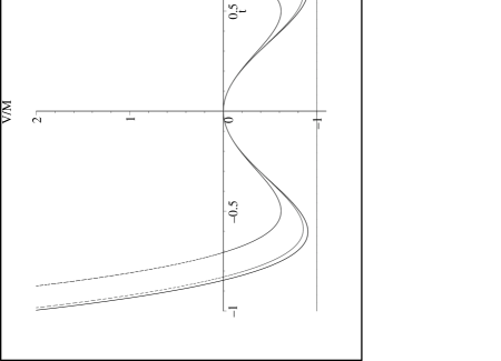
Figure 1: The effective tachyon potential in the three approximations.

$$g^{2}S_{0} = \textstyle\frac{1}{4}\,t^{2}-\textstyle\frac{1}{2}\,t^{4},$$

$$g^{2}S_{\textstyle\frac{3}{2}} = -a\,t^{2}-\textstyle\frac{1}{4}\,e\,t^{2}-\textstyle\frac{5}{96}\sqrt{50+22\sqrt{5}}e\,t^{4},$$

$$g^{2}S_{2} = {\displaystyle\textstyle\frac{15}{4}}\,{t^{3}v_{1}}-{\displaystyle\textstyle\frac{17}{6}}\,{t^{3}v_{2}}-{\displaystyle\textstyle\frac{1}{4}}\,{t^{3}v_{3}}+{\displaystyle\textstyle\frac{35}{12}}\,{t^{3}v_{4}}-{\displaystyle\textstyle\frac{11}{6}}\,{t^{3}v_{5}},$$

$$g^{2}S_{3} = 2\,a\,e+5\,f^{2}-\Bigl{(}\,\textstyle\frac{1}{\sqrt{2}}-\textstyle\frac{1}{24}\,\Bigr{)}\,e^{2}\,t^{2}+\textstyle\frac{5}{18}\,e^{2}\,t^{4}+\,\textstyle\frac{5}{4}(4\sqrt{2}\,-1)\,f^{2}\,t^{2}$$

$$+ \textstyle\frac{1}{12}\,(\,3+40\sqrt{2}\,)\,ae\,t^{2}-\textstyle\frac{5}{12}\,(\,10\sqrt{2}-1\,)ef\,t^{2}\,,$$

$$g^{2}S_{\textstyle\frac{7}{2}} = \mbox{}-{\displaystyle\textstyle\frac{25}{9}}\,{t\,a\,v_{1}}+{\displaystyle\textstyle\frac{44}{27}}\,{t\,a\,v_{2}}+{\displaystyle\textstyle\frac{44}{27}}\,{t\,a\,v_{3}}-{\displaystyle\textstyle\frac{329}{27}}\,{t\,a\,v_{4}}+{\displaystyle\textstyle\frac{64}{9}}\,{t\,a\,v_{5}}$$

$$- \mbox{}{\displaystyle\textstyle\frac{25}{36}}\,{t\,e\,v_{1}}+{\displaystyle\textstyle\frac{35}{27}}\,{t\,e\,v_{2}}-{\displaystyle\textstyle\frac{17}{18}}\,{t\,e\,v_{3}}-{\displaystyle\textstyle\frac{41}{108}}\,{t\,e\,v_{4}}+{\displaystyle\textstyle\frac{8}{27}}\,{t\,e\,v_{5}}$$

$$- \mbox{}{\displaystyle\textstyle\frac{80}{9}}\,{t\,f\,v_{1}}-{\displaystyle\textstyle\frac{80}{27}}\,{t\,f\,v_{3}}+{\displaystyle\textstyle\frac{160}{9}}\,{t\,f\,v_{4}}-{\displaystyle\textstyle\frac{320}{27}}\,{t\,f\,v_{5}}$$

$$+ 4.35732\,{t^{3}\,e\,v_{1}}-4.77364\,{t^{3}\,e\,v_{2}}+.605194\,{t^{3}\,e\,v_{3}}+4.351715\,{t^{3}\,e\,v_{4}}$$

$$- 1.94348\,{t^{3}\,e\,v_{5}},$$

$$g^{2}S_{4} = -\textstyle\frac{45}{8}\,{v_{1}}^{2}+3\,{v_{2}}^{2}+\textstyle\frac{3}{4}\,{v_{3}}^{2}-\textstyle\frac{15}{8}\,{v_{4}}^{2}-\textstyle\frac{3}{2}\,{v_{5}}^{2}+3\,{v_{4}}\,{v_{5}}$$

$$- {\displaystyle\textstyle\frac{945}{64}}\,t^{2}{v_{1}}^{2}-{\displaystyle\textstyle\frac{35}{6}}\,t^{2}{v_{2}}^{2}+{\displaystyle\textstyle\frac{5}{4}}\,t^{2}{v_{3}}^{2}\mbox{}-{\displaystyle\textstyle\frac{3511}{192}}t^{2}\,{v_{4}}^{2}-{\displaystyle\textstyle\frac{161}{24}}\,t^{2}{v_{5}}^{2}$$

$$+ {\displaystyle\textstyle\frac{255}{16}}\,t^{2}{v_{1}}\,{v_{2}}+{\displaystyle\textstyle\frac{45}{32}}\,t^{2}{v_{1}}\,{v_{3}}-{\displaystyle\textstyle\frac{525}{32}}\,t^{2}{v_{1}}\,{v_{4}}+{\displaystyle\textstyle\frac{165}{16}}\,t^{2}{v_{1}}\,{v_{5}}+{\displaystyle\textstyle\frac{19}{48}}\,t^{2}{v_{2}}\,{v_{3}}$$

$$+ \mbox{}{\displaystyle\textstyle\frac{991}{48}}t^{2}\,{v_{2}}\,{v_{4}}-{\displaystyle\textstyle\frac{143}{12}}\,t^{2}{v_{2}}\,{v_{5}}-{\displaystyle\textstyle\frac{65}{32}}\,t^{2}{v_{3}}\,{v_{4}}+{\displaystyle\textstyle\frac{7}{8}}\,t^{2}{v_{3}}\,{v_{5}}+{\displaystyle\textstyle\frac{985}{48}}\,t^{2}{v_{4}}\,{v_{5}}.$$

The potential is given by

$$V(t,a,e,f,v_{i})=-S(t,a,e,f,v_{i})=-2\pi^{2}M\,g^{2}S(t,a,e,f,v_{i})\,,$$

where $M=\frac{1}{2\pi^{2}g^{2}}$. The potential has a minimum for the following values of $t,a,e,f,v_{i}$.

$$t=\pm 0.603455,\,\,\,a=0.059291,\,\,\,e=0.030980,f=0.015746,\,\,\,v_{1}=\pm 0.035688,\,\,\,$$

$$v_{2}=\pm 0.0571190,\,\,\,v_{3}=\pm 0.0153737,\,\,\,v_{4}=\pm 0.031538,\,\,\,v_{5}=\mp 0.006012.$$

The value of the potential at the minimum is

$$V=-0.90454\,M\,.$$

The expected answer for the value of the potential at the minimum is $-M$. Thus we see that the level four approximation produces $90.5\%$ of the expected value. We can integrate out the fields $a,\,e,\,f,\,$ and $v_{\alpha}$ to obtain an effective potential for the tachyon which is given by

$$V_{effective}=-2\pi^{2}M\frac{P(t)}{Q(t)},$$

where

$$P(t) = 0.8168083768\,10^{-5}\,t^{2}+0.0002047077013\,t^{4}+0.002821258794\,t^{6}$$

$$+ 0.02594499700\,t^{8}+0.1738511409\,t^{10}+0.8795191385\,t^{12}$$

$$+ 3.409051376\,t^{14}+10.11847495\,t^{16}+22.58030878\,t^{18}$$

$$+ 35.88635644\,t^{20}+33.50595320\,t^{22}-4.683061411\,t^{24}$$

$$- 77.91238815\,t^{26}-149.1412411\,t^{28}-168.7145393\,t^{30}$$

$$- 125.0599362\,t^{32}-57.59279282\,t^{34}-12.56479811\,t^{36},$$

and

$$Q(t)=0.00003267233507+0.0008678393076\,t^{2}+0.01254363691\,t^{4}$$

$$+ 0.1215742201\,t^{6}+0.8648433845\,t^{8}+4.706706334\,t^{10}$$

$$+ 20.03806794\,t^{12}+67.54526560\,t^{14}+181.3752555\,t^{16}$$

$$+ 388.8655996\,t^{18}+664.8883542\,t^{20}+902.1103038\,t^{22}$$

$$+ 959.2815429\,t^{24}+778.5205080\,t^{26}+459.3896684\,t^{28}$$

$$+ 177.3949239\,t^{30}+33.42209885\,t^{32}.$$

4 Appendix

Conformal Transformations:

$$f\cdot T(0) = (f^{\prime}(0))^{-\frac{1}{2}}\,T(w)$$

$$f\cdot A(0) = f^{\prime}(0)\,\{A(w)-\textstyle\frac{f^{\prime\prime}(0)}{(f^{\prime}(0))^{2}}\,c\partial c\,\xi\,\partial\xi e^{-2\phi}(w)\,\}$$

$$f\cdot E(0) = f^{\prime}(0)\,\{E(w)-\textstyle\frac{f^{\prime\prime}(0)}{2(f^{\prime}(0))^{2}}\,\}$$

$$f\cdot F(0) = f^{\prime}(0)\,F(w)\,$$

$$f\cdot V_{1}(0) = (f^{\prime}(0))^{\frac{3}{2}}\,\{V_{1}(w)-\textstyle\frac{15}{12}\{z,f\}\xi\,c\,e^{-\phi}(w)\}$$

$$f\cdot V_{2}(0) = (f^{\prime}(0))^{\frac{3}{2}}\,\{V_{2}(w)-\textstyle\frac{f^{\prime\prime}(0)}{(f^{\prime}(0))^{2}}\xi\partial c\,e^{-\phi}(w)+(2\frac{{(f^{\prime\prime}(0))^{2}}}{{(f^{\prime}(0))^{4}}}-\frac{{f^{\prime\prime\prime}(0)}}{{(f^{\prime}(0))^{3}}})\xi ce^{-\phi}(w)\,\}$$

$$f\cdot V_{3}(0) = (f^{\prime}(0))^{\frac{3}{2}}\,\{V_{3}(w)+\textstyle\frac{1}{6}\,\{z,f\}\,\xi\,c\,e^{-\phi}(w)+\frac{f^{\prime\prime}(0)}{2(f^{\prime}(0))^{2}}\partial\xi ce^{-\phi}\,\}$$ (25)

$$f\cdot V_{4}(0) = (f^{\prime}(0))^{\frac{3}{2}}\,\{V_{4}(w)-\textstyle\frac{1}{2}\textstyle\frac{f^{\prime\prime}(0)}{(f^{\prime}(0))^{2}}\xi c\partial\phi e^{-\phi}+(\textstyle\frac{1}{12}\textstyle\frac{f^{\prime\prime\prime}(0)}{(f^{\prime}(0))^{3}}-\textstyle\frac{2}{3}\{z,f\})\,\xi\,c\,e^{-\phi}(w)\,\}$$

$$f\cdot V_{5}(0) = (f^{\prime}(0))^{\frac{3}{2}}\,\{V_{5}(w)+\textstyle\frac{f^{\prime\prime}(0)}{(f^{\prime}(0))^{2}}\xi c\partial\phi e^{-\phi}+(\textstyle\frac{1}{2}\{z,f\}-\textstyle\frac{1}{6}\textstyle\frac{f^{\prime\prime\prime}(0)}{(f^{\prime}(0))^{3}})\xi ce^{-\phi}\}$$

$${\cal P}^{I}_{A} = -\textstyle\frac{f^{\prime\prime}_{I}(0)}{(f^{\prime}_{I}(0))^{2}}\,,\,{\cal P}_{E}^{I}=-\textstyle\frac{f^{\prime\prime}_{I}(0)}{2(f^{\prime}_{I}(0))^{2}}\,,\,{\cal P}_{F}^{I}=0$$ (26)

$${\cal P}^{I}_{V_{1}} = 0\,,\,{\cal P}^{I}_{V_{2}}=-\textstyle\frac{f^{\prime\prime}_{I}(0)}{(f^{\prime}_{I}(0))^{2}}\,,\,{\cal P}^{I}_{V_{3}}=\textstyle\frac{f^{\prime\prime}_{I}(0)}{2(f^{\prime}_{I}(0))^{2}}\,,\,{\cal P}^{I}_{V_{4}}=-\textstyle\frac{f^{\prime\prime}_{I}(0)}{2(f^{\prime}_{I}(0))^{2}}\,,\,{\cal P}^{I}_{V_{5}}=\textstyle\frac{f^{\prime\prime}_{I}(0)}{(f^{\prime}_{I}(0))^{2}}\,,\,$$ (27)

$${\cal R}^{I}_{V_{1}} = -\textstyle\frac{15}{12}\{z,f\}\,,\,{\cal R}^{I}_{V_{2}}=2\frac{{(f^{\prime\prime}(0))^{2}}}{{(f^{\prime}(0))^{4}}}-\frac{{f^{\prime\prime\prime}(0)}}{{(f^{\prime}(0))^{3}}}\,,\,{\cal R}^{I}_{V_{3}}=\textstyle\frac{1}{6}\{z,f\}\,,$$ (28)

$${\cal R}^{I}_{V_{4}} = \textstyle\frac{1}{12}\textstyle\frac{f^{\prime\prime\prime}(0)}{(f^{\prime}(0))^{3}}-\textstyle\frac{2}{3}\{z,f\}\,,\,{\cal R}^{I}_{V_{5}}=-\textstyle\frac{1}{6}\textstyle\frac{f^{\prime\prime\prime}(0)}{(f^{\prime}(0))^{3}}+\textstyle\frac{1}{2}\{z,f\}\,,\,$$ (29)

BRST transformations:

$$Q_{B}=\oint dzj_{B}(z)=\oint dz\Bigl{\{}c\bigl{(}T_{m}+T_{\xi\eta}+T_{\phi})+c\partial cb+\eta\,e^{\phi}\,G_{m}-\eta\partial\eta e^{2\phi}b\Bigr{\}}\,,$$

$$Q_{0} \equiv \oint dz\Bigl{\{}c\bigl{(}T_{m}+T_{\xi\eta}+T_{\phi})+c\partial cb,$$

$$Q_{1} \equiv \oint dz\,\eta e^{\phi}G_{m}\,\,\,,\,\,\,Q_{2}\equiv-\oint dz\,\eta\partial\eta e^{2\phi}b.$$

$$U_{2}=\xi\partial ce^{-\phi},\,\,\,U_{3}=\partial\xi ce^{-\phi},\,\,\,U_{4}=U_{5}=\xi c\partial\phi e^{-\phi}.$$

$Q_{0}$:

$$Q_{0}(T) = -\textstyle\frac{1}{2}\xi c\partial ce^{-\phi},$$

$$Q_{0}(A) = -2c\partial c\partial^{2}c\xi\partial\xi e^{-2\phi},$$

$$Q_{B}(E) = c\partial\xi\eta-\partial c\eta\xi-c\partial\eta\xi-\textstyle\frac{1}{2}\partial^{2}c+\eta e^{\phi}G_{m}+2\partial\eta\eta e^{2\phi}b,$$

$$Q_{B}(F) = \partial c\xi cG_{m}e^{-\phi},$$

$$Q_{0}(V_{1}) = \textstyle\frac{c_{m}}{2}\textstyle\frac{1}{3!}\partial^{3}c\xi ce^{-\phi}+\textstyle\frac{3}{2}\partial c\xi cT_{m}e^{-\phi}\,,$$

$$Q_{0}(V_{2}) = -\partial\xi c\partial^{2}ce^{-\phi}-\textstyle\frac{3}{2}\xi\partial c\partial^{2}ce^{-\phi}-\xi c\partial^{3}ce^{-\phi}+c\xi\partial^{2}c\partial e^{-\phi},$$

$$Q_{0}(V_{3}) = \textstyle\frac{c_{\xi\eta}}{2}\textstyle\frac{1}{3!}\partial^{3}c\xi ce^{-\phi}+\textstyle\frac{3}{2}c\partial c\xi T_{\xi\eta}e^{-\phi}+\textstyle\frac{1}{2}c\partial^{2}c\partial\xi e^{-\phi}\,,$$

$$Q_{0}(V_{4}) = \textstyle\frac{9}{12}\partial^{3}c\xi ce^{-\phi}+\textstyle\frac{3}{2}\partial c\xi T_{\phi}ce^{-\phi}+\textstyle\frac{1}{2}\xi\partial^{2}cc\partial\phi e^{-\phi}\,,$$

$$Q_{0}(V_{5}) = -\textstyle\frac{2}{3}\partial^{3}c\xi c+\xi c\partial^{2}c\partial\phi e^{-\phi}+\textstyle\frac{3}{2}\xi c\partial c\partial^{2}\phi e^{-\phi},$$

$$Q_{0}(U_{A}) = 0\,,$$

$$Q_{0}(U_{2}) = \partial(c\xi\partial ce^{-\phi}),$$

$$Q_{0}(U_{3}) = \textstyle\frac{1}{2}\partial\xi c\partial ce^{-\phi},$$

$$Q_{0}(U_{4}) = \textstyle\frac{1}{2}c\partial c\xi\partial\phi e^{-\phi}-\frac{1}{2}c\partial^{2}c\xi e^{-\phi}.$$

$$c_{m}=15,\,\,\,\,\,\,\,\,\,\,\,\,\,\,\,\,\,\,\,\,\,\,\,c_{\xi\eta}=-2.$$

$Q_{1}$:

$$Q_{1}(F) = -10\partial\eta\,\xi c-10\eta\xi c(\partial\phi)-2T_{m}c\partial\phi-5(\partial^{2}\phi+(\partial\phi)^{2})c,$$

$$Q_{1}(V_{1}) = \textstyle\frac{3}{2}\xi\eta cG_{m}-\textstyle\frac{3}{2}cG_{m}\partial\phi-\textstyle\frac{1}{2}c\partial G_{m}\,,$$

$$Q_{1}(V_{2}) = 0,$$

$$Q_{1}(V_{3}) = \xi\eta cG_{m},$$

$$Q_{1}(V_{4}) = -\textstyle\frac{3}{2}G_{m}\eta\xi c-\textstyle\frac{5}{2}G_{m}\partial\phi c-\textstyle\frac{3}{2}\partial G_{m}c,$$

$$Q_{1}(V_{5}) = G_{m}\eta\xi c+\partial G_{m}c+G_{m}\partial\phi c,$$

$$Q_{1}(U_{2}) = 0,$$

$$Q_{1}(U_{3}) = G_{m}c,$$

$$Q_{1}(U_{4}) = G_{m}c.$$

$Q_{2}$:

$$Q_{2}(T) = -\eta e^{\phi},$$

$$Q_{2}(V_{1}) = -\eta e^{\phi}T_{m},$$

$$Q_{2}(V_{2}) = 2\eta\partial\eta\xi e^{\phi}-3\partial^{2}\eta e^{\phi}-8\partial\eta\partial\phi e^{\phi}-2\eta\partial^{2}\phi e^{\phi}-4\eta(\partial\phi)^{2}e^{\phi},$$

$$Q_{2}(V_{3}) = \eta\partial bce^{\phi}+2\eta bc(\partial\phi)e^{\phi}+3\partial\eta\xi\eta e^{\phi}+\eta\partial^{2}\phi e^{\phi}+2\eta(\partial\phi)^{2}e^{\phi},$$

$$Q_{2}(V_{4}) = -4\eta\partial\eta\xi e^{\phi}+8\partial\eta bce^{\phi}+4\eta\partial bce^{\phi}+10\eta bc\partial\phi e^{\phi},$$

$$+ 6\partial^{2}\eta e^{\phi}+20\partial\eta\partial\phi e^{\phi}+5\eta\partial^{2}\phi e^{\phi}+\textstyle\frac{25}{2}\eta(\partial\phi)^{2}e^{\phi},$$

$$Q_{2}(V_{5}) = 2\eta\partial\eta\xi e^{\phi}-4\partial\eta bce^{\phi}-2\eta\partial bce^{\phi}-4\eta bc\partial\phi e^{\phi}-3\partial^{2}\eta e^{\phi}-8\partial\eta\partial\phi e^{\phi},$$

$$- 3\eta\partial^{2}\phi e^{\phi}-4\eta(\partial\phi)^{2}e^{\phi},$$

$$Q_{2}(U_{3}) = -2\eta bce^{\phi}-3\partial\eta e^{\phi}-4\eta\partial\phi e^{\phi},$$

$$Q_{2}(U_{2}) = -2\partial(\eta e^{\phi}),$$

$$Q_{2}(U_{4}) = -2\eta bce^{\phi}-5\eta\partial\phi e^{\phi}-4\partial\eta e^{\phi}.$$

References

• [1] O. Bergman and M. R. Gaberdiel, “Stable non-BPS D-particles,” Phys. Lett.  B441, 133 (1998), hep-th/9806155.
• [2] A. Sen, “SO(32) spinors of type I and other solitons on brane-antibrane pair,” JHEP 9809, 023 (1998), hep-th/9808141.
• [3] A. Sen, “Type I D-particle and its interactions,” JHEP 9810, 021 (1998), hep-th/9809111.
• [4] A. Sen, “BPS D-branes on non-supersymmetric cycles,” JHEP 9812, 021 (1998) [hep-th/9812031].
• [5] A. Sen, “Stable non-BPS bound states of BPS D-branes,” JHEP 9808, 010 (1998), hep-th/980519.
• [6] A. Sen, “Tachyon condensation on the brane antibrane system,” JHEP 9808, 012 (1998), hep-th/9805170.
• [7] N. Berkovits, “The Tachyon Potential in Open Neveu-Schwarz String Field Theory”, hep-th/0001084.
• [8] N. Berkovits, A. Sen and B. Zwiebach, “Tachyon condensation in superstring field theory,” hep-th/0002211.
• [9] N. Berkovits, “Super-Poincare Invariant Superstring Field Theory,” Nucl. Phys. B450 (1995) 90, hep-th/9503099.
• [10] N. Berkovits, “A New Approach to Superstring Field Theory,” proceedings to the $32^{nd}$ International Symposium Ahrenshoop on the Theory of Elementary Particles, Fortschritte der Physik (Progress of Physics) 48 (2000) 31, hep-th/9912121.
• [11] D. Friedan, E. Martinec, and S. Shenker, “Conformal Invariance, Supersymmetry, and String Theory,” Nucl. Phys. B271 (1986) 93.
• [12] A. Sen, “Universality of Tachyon Potential”, JHEP 9912, 027 (1999) hep-th/9911116.
• [13] P. De Smet, J. Raemaekers, “Level Four Approximation to the Tachyon Potential in Superstring field Theory”, hep-th/0003320.