Stretched Strings in Noncommutative Field Theory

Abstract:

Motivated by recent discussions of IR/UV mixing in noncommutative field theories, we perform a detailed analysis of the non-planar amplitudes of the bosonic open string in the presence of an external $B$-field at the one-loop level. We carefully isolate, at the string theory level, the contribution which is responsible for the IR/UV behavior in the field theory limit. We show that it is a pure open string effect by deriving it from the factorization of the one-loop amplitude into the disk amplitudes of intermediate open string insertions. We suggest that it is natural to understand IR/UV mixing as the creation of intermediate “stretched strings”.

1 Introduction

Noncommutative field theory has recently received a lot of attention from string theorists. The appearance of noncommutative geometry in string theory was first made clear in [1, 2] (for earlier work see [3]). Subsequently, it was shown in [4] that noncommutative gauge theories will generically arise from open string theory in the presence of a constant Neveu-Schwarz $B$-field. More recently, it has been shown [5] that perturbative noncommutative field theories [6] exhibit an intriguing IR/UV mixing.

The mixing of IR and UV degrees of freedom may be seen in many different ways. By thinking of field theory quanta as pairs of dipoles moving in a magnetic field [4, 7, 8, 9, 10], one understands that the relative position of the dipole is proportional to the center of mass momentum. Alternatively, the mixing follows simply from the nature of the star product [5]; e.g.

$$\delta(x)\ast\delta(x)=\text{const}.$$ (1)

The UV/IR mixing also allows for interesting soliton solutions that would otherwise be prohibited by Derrick’s theorem [11].

Perhaps one of the most interesting manifestations of the IR/UV mixing is the behaviour, first uncovered at one loop level in [5], of non-planar loop integrals in scalar field theories, which has since been generalized to higher loops [12] and to many other theories [13, 14, 15, 16, 17, 18, 10, 19, 20, 21]. One of the key elements in all these theories is the emergence of a factor

$$\exp[-{p\circ p\over t}]; \qquad p\circ p\equiv-p_{\mu}\left(\Theta^{2}\right)^{\mu\nu}p_{\nu},$$ (2)

in the integral over the Schwinger parameter $t$, after the loop momentum integration. With non-zero external non-planar momentum $p$, this factor regularizes otherwise divergent integrals. For this reason, it has been suspected that non-planar diagrams (not including planar sub-diagrams which can be renormalized) are finite; then the whole theory would be renormalizable. However, in [5] it was found that there are actually infrared singularities, associated with the factor (2) at $p=0$, in the diagrams that were UV divergent for $\Theta=0$. This is easily understood by thinking of $p\circ p$ as a short distance cutoff of the theory; taking $p=0$ corresponds to removing the cutoff. If we introduce a UV cutoff $\Lambda$ in the theory, then the $p\rightarrow 0$ and $\Lambda\rightarrow\infty$ limits do not commute and the theory does not appear to have a consistent Wilsonian description.

It has been suggested in [5, 12] that the IR singularity may be associated with missing new light degrees of freedom in the theory. There it was shown that by adding new fields to the action with appropriate form, the IR singularities in the 1-loop effective action of certain scalar field theories can indeed be reproduced and might result in a consistent Wilsonian action. It was further suggested, with the observation that $-\Theta^{2}$ looks like the closed string metric in the decoupling limit, that this procedure is an analog of the open string theory factorization into closed string particles.

The purpose of this paper is two-fold. Since noncommutative field theory can generally be reduced from string theory on a D-brane with a background $B$-field [2, 22, 23, 24, 25, 4] we try to identify the string theory origin of the IR/UV behavior. In particular, we examine whether the above-mentioned effect can be attributed to closed string modes, or the non-decoupling of other massive open string modes. Our other motivation is that we would like to provide another intriguing example of IR/UV mixing at the string theory level. We point out that in the presence of a $B$-field the open string generically has a finite winding mode proportional to its momentum. We argue that this effect persists at the field theory level, and offers a simple explanation of the IR singularities of the non-planar diagrams.

More explicitly, by examining the one-loop string amplitude and its reduction to field theory, we will show that the occurrence of (2) and its associated IR singularities is an open string phenomenon, and does not involve closed strings. In particular we will see that the $-\Theta^{2}$ appearing in (2) does not originate from the closed string metric at the string theory level. Rather, if we write $x^{\mu}=\Theta^{\mu\nu}p_{\nu}$, then $p\circ p=x^{\mu}G_{\mu\nu}x^{\nu}$, where $G_{\mu\nu}$ is the open string metric. We will argue in section 3 that it is natural to interpret $x^{\mu}$ as a spacetime distance of a stretched string and that therefore the factor (2) is just $e^{-x^{2}/t}$, corresponding to a specific type of short-distance regularization of the field theory.

This paper is organized as follows. In section 2, we introduce our notation, and write down the one-loop amplitude for scattering of open string tachyons in a background $B$-field. To further illustrate the structure of the amplitude, in section 2.1, we discuss the open string factorization in the short cylinder limit. In section 2.2, we discuss the closed string factorization in the long cylinder limit. Having understood the structure of the amplitude, we are then able to able to derive our understanding of the IR/UV mixing of [5], in section 3. Section 4 contains our discussion and conclusions.

2 The One-Loop Amplitude

In this section we compute the one-loop scattering amplitudes for $M$ tachyons in the presence of a background $B$-field in the open bosonic string theory. We focus on the tachyons without Chan-Paton factors for simplicity; however, since our arguments and results can be traced to general properties of the Green function and conformal field theory, we expect our conclusions to hold more generally. We will mostly focus on the non-planar amplitudes, although the planar amplitudes can also be read from our results. It is also easy to insert Chan-Paton factors.

The open string action is (in conformal gauge)

$$S=\frac{1}{4\pi\alpha^{\prime}}\int d^{2}z\left\{g_{\mu\nu}\partial_{a}X^{\mu}\partial^{a}X^{\nu}-i\varepsilon^{ab}B_{\mu\nu}\partial_{a}X^{\mu}\partial_{b}X^{\nu}\right\}+\frac{i}{2\pi\alpha^{\prime}}\oint d\tau A_{\mu}\partial_{\tau}X^{\mu}.$$ (3)

We effectively set $F=dA$ to zero, by absorbing $F$ into $B$—this can be considered either a notational convenience or the result of a gauge transformation. The action (3) is exact in $\alpha^{\prime}$, because we consider only constant background fields. This action leads to the boundary condition

$$\left.{g_{\mu\nu}\partial_{n}X^{\nu}-iB_{\mu\nu}\partial_{\tau}X^{\nu}}\right|_{\text{bdy}}=0,$$ (4)

where $\partial_{n}$ and $\partial_{\tau}$ are respectively normal and tangential derivatives.

The Green function for the bosonic open string on the annulus, in the presence of a $B$-field, was originally given in [34, 35, 36]. In the coordinate system in which the world-sheet is a flat annulus with inner radius $a$ and unit outer radius (figure 1), it can be written as

$${\mathcal{G}}^{\mu\nu}(z,z^{\prime})={\left\langle{X^{\mu}(z)X^{\nu}(z^{\prime})}\right\rangle}=-\frac{\alpha^{\prime}}{2}\Bigl{[}g^{\mu\nu}\ln\left\lvert{Z}\right\rvert^{2}+\Bigl{(}\frac{g-B}{g+B}\Bigr{)}^{\mu\nu}\ln Y+\Bigl{(}\frac{g+B}{g-B}\Bigr{)}^{\mu\nu}\ln\bar{Y}\Bigr{]}$$ (5)

where

Figure 1: The annulus.

$$Z =\frac{ia^{\frac{1}{6}}}{\eta(\tau)}\sqrt{zz^{\prime}}\vartheta_{11}(\nu,\tau), Y =\frac{ia^{\frac{1}{6}}}{\eta(\tau)}\sqrt{z\bar{z}^{\prime}}\vartheta_{11}(\mu,\tau),$$ (6a)

with

$$a^{2} =e^{2\pi i\tau}, e^{2\pi i\nu} =\frac{z^{\prime}}{z}, e^{2\pi i\mu} =z\bar{z}^{\prime}.$$ (6b)

Note in (5) the indices are raised and lowered by $g_{\mu\nu}$. We closely follow the conventions of [37] for the definitions of the Jacobi-$\vartheta$ and Dedekind-$\eta$ functions.

Figure 2: The conformally equivalent description of the annulus as a cylinder.

The Green function satisfies

$$\partial\bar{\partial}{\mathcal{G}}_{\mu\nu}(z,z^{\prime})=-\pi\alpha^{\prime}g_{\mu\nu}\delta^{(2)}(z-z^{\prime}),$$ (7a)

and

$$\left[\partial_{n}{\mathcal{G}}_{\mu\nu}(z,z^{\prime})-iB_{\mu}{{}^{\lambda}}\partial_{\tau}{\mathcal{G}}_{\lambda\nu}(z,z^{\prime})\right]_{\left\lvert{z}\right\rvert=a,1}=\begin{cases}0,&\left\lvert{z}\right\rvert=a\\ -\alpha^{\prime}g_{\mu\nu},&\left\lvert{z}\right\rvert=1\end{cases}.$$ (7b)

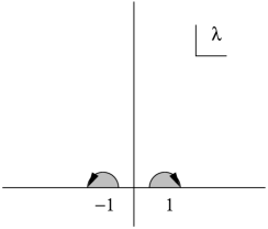
Figure 3: The annulus as an upper half-plane, minus two regions with identified boundaries.

Equation (7b) is almost a consequence of equation (4); it differs from it on one boundary as a result of Gauss’ law, for otherwise equation (7a) would be incompatible with equation (7b). We could follow [37] and subtract a background charge from the Green function instead of modifying the boundary condition; however, this will not affect amplitudes. Indeed, we will often in the following, drop, with neither warning nor explanation, terms in the Green function of the form $f_{\mu\nu}(z,\bar{z})+h_{\mu\nu}(z^{\prime},\bar{z}^{\prime})$, as momentum conservation prevents such terms from contributing to on-shell amplitudes.

It will often be more convenient to use other coordinate systems. The cylindrical coordinate (figure 2) is

$$\begin{aligned} w&=\sigma+i\tau\end{aligned};\qquad\begin{aligned} \sigma&\in[0,\pi]\\ \tau&\in[0,2\pi t)\end{aligned};\qquad\begin{aligned} w\sim w+2\pi it,\end{aligned}$$ (8)

where ${\mathbb{{R}}}\ni t>0$ is the modulus. The relation between the cylinder and the annulus is

$$z =e^{-{w\over t}}, a =e^{-\frac{\pi}{t}}.$$ (9)

The coordinate on the upper half-plane is

$$\lambda=i\tan\frac{w-i\pi t}{2}.$$ (10)

$\lambda$ maps the cylinder to the upper half plane with two identified semi-circles removed, each being bounded by a segment of the real axis—see figure 3. As $t\rightarrow\infty$, the semi-circles become infinitely small, and centred at $\lambda=\pm 1$.

When restricting to the boundary of the cylinder, the propagator becomes (in cylindrical coordinates),

$${\mathcal{G}}^{\mu\nu}(i\tau_{1},i\tau_{2})=-\alpha^{\prime}G^{\mu\nu}\ln\left\lvert{\vartheta_{11}\bigl{(}\frac{\tau_{12}}{2\pi t},\frac{i}{t}\bigr{)}}\right\rvert^{2}+\frac{i}{2}\Theta^{\mu\nu}\bigl{[}\frac{\tau_{12}}{\pi t}-\epsilon(\tau_{12})\bigr{]},$$ (11a)

$${\mathcal{G}}^{\mu\nu}(\pi+i\tau_{1},\pi+i\tau_{2})=\alpha^{\prime}g^{\mu\nu}{\pi\over t}-\alpha^{\prime}G^{\mu\nu}\ln\left\lvert{\vartheta_{11}\bigl{(}\frac{\tau_{12}}{2\pi t},\frac{i}{t}\bigr{)}}\right\rvert^{2}-\frac{i}{2}\Theta^{\mu\nu}\bigl{[}\frac{\tau_{12}}{\pi t}-\epsilon(\tau_{12})\bigr{]},$$ (11b)

$${\mathcal{G}}^{\mu\nu}(\pi+i\tau_{1},i\tau_{2})=-\alpha^{\prime}G^{\mu\nu}\ln\left\lvert{e^{-\frac{\pi}{4t}}\vartheta_{01}\bigl{(}\frac{\tau_{1}-\tau_{2}}{2\pi t},\frac{i}{t}\bigl{)}}\right\rvert^{2},$$ (11c)

where $\tau_{12}=\tau_{1}-\tau_{2}$ and we have defined, following [4],

$$G^{\mu\nu} =\big{(}{1\over g+B}g{1\over g-B}\big{)}^{\mu\nu}=\big{(}{1\over g+B}\big{)}_{S}^{\mu\nu},$$ (12a)

$$G_{\mu\nu} =g_{\mu\nu}-(Bg^{-1}B)_{\mu\nu},$$ (12b)

$$\Theta^{\mu\nu} =-(2\pi\alpha^{\prime})\big{(}{1\over g+B}B{1\over g-B}\big{)}^{\mu\nu}=2\pi\alpha^{\prime}\big{(}{1\over g+B}\big{)}_{A}^{\mu\nu},$$ (12c)

where the subscript $S$ ($A$) denotes the (anti)symmetric part of the matrix. Also, $\epsilon(\tau)=\tau/\left\lvert{\tau}\right\rvert$ is the sign of $\tau$, and we recall from e.g. [4] that $g_{\mu\nu}$ is the closed string metric and $G_{\mu\nu}$ is the open string metric (with inverse $G^{\mu\nu}$). $\Theta^{\mu\nu}$ is an open string noncommutativity parameter. Conversely, the closed string parameters $g,B$ may be expressed in terms of the open string parameters $G,\Theta$ as

$$g+B=\left(\frac{1}{G^{-1}+\frac{1}{2\pi\alpha^{\prime}}\Theta}\right)_{\mu\nu}.$$ (13)

In particular,

$$g^{\mu\nu}=G^{\mu\nu}-\left(\frac{1}{2\pi\alpha^{\prime}}\right)^{2}(\Theta G\Theta)^{\mu\nu}.$$ (14)

We notice that the boundary Green functions on the cylinder have some interesting new features compared to those of the disk [35, 36] and those in the well-known case of $B=0$. In (11b) the dependence on the closed string metric does not drop out completely. We shall see later that this is essential for the non-planar amplitudes to factorize into the closed string channel in the long cylinder limit ($t\rightarrow 0$). There is an additional dependence on $\Theta$ proportional to the distance between the two points. These linear terms will drop out in the planar amplitudes due to momentum conservation but will be important in non-planar amplitudes. It is easy to see that planar amplitudes will mimic those of $B=0$ except for additional phase factors associated with external momenta.

Using the boundary Green functions (11a)–(11c), we now write down the non-planar amplitude for $M$ tachyons with $N$ attached to the $\sigma=0$ boundary and $M-N$ to the $\sigma=\pi$ boundary. The vertex operators on the $\sigma=0$ boundary will be labeled by $i,j,\dots=1,\dots,N$ and those on the $\sigma=\pi$ boundary by $r,s,\dots=N+1,\dots,M$. $p,q$ go from $1$ to $M$. The normalized open string tachyon vertex operator is ${\cal V}_{i}=g_{o}e^{ik_{i\mu}X^{\mu}}$, where $g_{o}$ is the open string coupling. We also define

$$k_{i}\cdot k_{j} =k_{i\mu}G^{\mu\nu}k_{j\nu}, k_{i}\times k_{j} =k_{i\mu}\Theta^{\mu\nu}k_{j\nu}.$$ (15)

The non-planar momentum—i.e. the momentum that flows between the two boundaries—is

$$k=\sum_{i=1}^{N}k_{i}=-\sum_{r=N+1}^{M}k_{r}.$$ (16)

In terms of the open string modular parameter $t$, the amplitude is

$$\begin{split}&S_{C^{2}}(1,\cdots,N;N+1,\cdots,M)=\int_{0}^{\infty}{dt\over 2t}{\left\langle{b(0)c(0)\prod_{i=1}^{N}\oint{\cal V}_{i}(i\tau_{i})\prod_{r=N+1}^{M}\oint{\cal V}_{r}(\pi+i\tau_{r})}\right\rangle}_{C^{2}}\\ &\quad=i\sqrt{\det G}\,g_{o}^{M}\,(2\pi)^{d}\,\delta^{(d)}\Bigl{(}\text{\small$\sum_{p=1}^{M}$}k_{p}\Bigr{)}\int_{0}^{\infty}\frac{dt}{2t}\,(8\pi^{2}\alpha^{\prime}t)^{-\frac{d}{2}}\,\eta(it)^{-24}\,\left[\prod_{p=1}^{M}\int_{0}^{2\pi t}d\tau_{p}\right]\Psi_{1}\Psi_{2}\Psi_{12}\\ &\quad\quad\times\exp\left[-\frac{\pi}{2t}\alpha^{\prime}k_{\mu}(g^{-1}-G^{-1})^{\mu\nu}k_{\nu}\right]e^{-\frac{i}{2}\sum_{i<j}(k_{i}\times k_{j})[\frac{\tau_{ij}}{\pi t}-\epsilon(\tau_{ij})]+{i\over 2}\sum_{r<s}(k_{r}\times k_{s})[\frac{\tau_{rs}}{\pi t}-\epsilon(\tau_{rs})]},\end{split}$$ (17)

where we consider $d=26$, but equation (LABEL:ampop) would hold on a D$(p{=}d{-}1)$-brane with no transverse momentum, for general $d$, corresponding to a $d$-dimensional field theory,

$$\begin{aligned} \Psi_{1}&=\prod_{i<j}\left\lvert{\psi_{ij}}\right\rvert^{2\alpha^{\prime}k_{i}\cdot k_{j}},&\Psi_{2}&=\prod_{r<s}\left\lvert{\psi_{rs}}\right\rvert^{2\alpha^{\prime}k_{r}\cdot k_{s}},&\Psi_{12}&=\prod_{i,r}(\psi^{T}_{ir})^{2\alpha^{\prime}k_{r}\cdot k_{i}},\end{aligned}$$ (18a)

$$\begin{aligned} \psi_{ij}&=-2\pi i\exp\left(-\frac{\tau_{ij}^{2}}{4\pi t}\right)\frac{\vartheta_{11}(i\frac{\tau_{ij}}{2\pi},it)}{\vartheta_{11}^{\prime}(0,it)},&\psi_{ir}^{T}&=2\pi\exp\left(-\frac{\tau_{ir}^{2}}{4\pi t}\right)\,\frac{\vartheta_{10}(i\frac{\tau_{ir}}{2\pi},it)}{\vartheta_{11}^{\prime}(0,it)}.\end{aligned}$$ (18b)

By a modular transformation of the $\vartheta$-functions we can also express the above amplitude in terms of the closed string modular parameter $s={\pi\over t}$. This gives

$$\begin{split}&S_{C^{2}}(1,\cdots,N;N+1,\cdots,M)=i\sqrt{\det G}\,g_{o}^{M}\,(8\pi^{2}\alpha^{\prime})^{-\frac{d}{2}}\,(2\pi)^{d}\,\delta^{(d)}\Bigl{(}\text{\small$\sum_{p=1}^{M}$}k_{p}\Bigr{)}\\ &\quad\times\int_{0}^{\infty}\frac{ds}{2}\,\Bigl{(}\frac{\pi}{s}\Bigr{)}^{13-\frac{d}{2}}\eta(\frac{is}{\pi})^{-24}\,\exp\big{[}-\frac{\alpha^{\prime}}{2}sk_{\mu}g^{\mu\nu}k_{\nu}\big{]}\left[\prod_{p=1}^{M}\int_{0}^{1}d\nu_{p}\right]\tilde{\Psi}_{1}\tilde{\Psi}_{2}\tilde{\Psi}_{12}\\ &\quad\times\exp\left[-\frac{i}{2}\sum_{i<j}(k_{i}\times k_{j})[2\nu_{ij}-\epsilon(\nu_{ij})]+\frac{i}{2}\sum_{r<s}(k_{r}\times k_{s})[2\nu_{rs}-\epsilon(\nu_{rs})]\right],\end{split}$$ (19)

with

$$\begin{aligned} \tilde{\Psi}_{1}&=\prod_{i<j}\left\lvert{\tilde{\psi}_{ij}}\right\rvert^{2\alpha^{\prime}k_{i}\cdot k_{j}},&\tilde{\Psi}_{2}&=\prod_{r<s}\left\lvert{\tilde{\psi}_{rs}}\right\rvert^{2\alpha^{\prime}k_{r}\cdot k_{s}},&\tilde{\Psi}_{12}&=\prod_{i,r}(\tilde{\psi}^{T}_{ir})^{2\alpha^{\prime}k_{r}\cdot k_{i}},\end{aligned}$$ (20a)

$$\begin{aligned} \tilde{\psi}_{ij}&=\frac{\vartheta_{11}(\nu_{ij},\frac{is}{\pi})}{\vartheta^{\prime}_{11}(0,\frac{is}{\pi})},&\tilde{\psi}_{ir}^{T}&=e^{-\frac{s}{4}}\frac{\vartheta_{01}(\nu_{ir},\frac{is}{\pi})}{\vartheta^{\prime}_{11}(0,\frac{is}{\pi})},\end{aligned}$$ (20b)

where for convenience we have defined $\nu_{i}=\frac{\tau_{i}}{2\pi t}$.

We make several remarks:

1. $\psi$ and $\tilde{\psi}$ have been defined to not contain any factors of $\exp\bigl{(}\frac{\pi}{t}\bigr{)}$. They do include $\vartheta$-functions, which encode the contributions of intermediate oscillation modes running in the loop, and do not depend on the $B$-field.

2. The $k_{i}\times k_{j}$ contribution to the amplitude comes directly from the $\Theta$ term in the propagators.

3. The structural differences of both (LABEL:ampop) and (19) with those in the $B=0$ case indicate that the introduction of non-zero $B$ affects only the zero (i.e. non-oscillator) modes of the intermediate state running in the loop. This can also be deduced from the fact that in the mode expansion of $X^{\mu}$ on the disk, $B$ does not affect commutators involving the oscillation modes.

4. In equation (LABEL:ampop) there is an exponential factor

   $$\exp\left[-\frac{\pi}{2t}\alpha^{\prime}k_{\mu}\bigl{(}g^{-1}-G^{-1}\bigr{)}^{\mu\nu}k_{\nu}\right]=\exp\left[\frac{1}{8\pi\alpha^{\prime}t}k_{\mu}(\Theta G\Theta)^{\mu\nu}k_{\nu}\right],$$ (21)

   using equation (14). The field theory limit of equation (LABEL:ampop) is obtained by taking

   $$\alpha^{\prime} \rightarrow 0, t \rightarrow\infty, \alpha^{\prime}t =\text{finite}, \alpha^{\prime}\tau_{p} =\text{finite}.$$ (22)

   In this limit the contributions from oscillators in (LABEL:ampop) drop out. The open string modulus $\alpha^{\prime}t$ and vertex coordinates $\alpha^{\prime}\tau_{p}$ become the Schwinger parameters of the corresponding $\Phi^{3}$ field theory with coupling constant $\frac{g_{o}}{\alpha^{\prime}}$. The factor (21) does not arise in the $B=0$ case. But precisely this factor carries over to noncommutative field theory, where it regularizes otherwise divergent diagrams while introducing IR/UV mixing. We emphasize that this is a very general phenomenon, not restricted to the $\Phi^{3}$ amplitudes explicitly considered here. For example, precisely the same factor appears if we replace the external legs by vector vertex operators relevant to gauge theory amplitudes, or if we reduce (LABEL:ampop) to $\Phi^{4}$ amplitudes using a slightly different scaling [32]. The tensor with which the non-planar momenta are contracted,

   $$\tilde{g}^{\mu\nu}=-(\Theta G\Theta)^{\mu\nu},$$ (23)

   was generally interpreted in noncommutative field theory discussions as the closed string metric in the $\alpha^{\prime}\rightarrow 0$ limit. However, we see here that at the string theory level (finite $\alpha^{\prime}$) this is not the closed string metric, and it arises from open string modes. In section 3 we shall give an explanation of its origin.

5. In terms of the closed string modulus, we have an exponential factor

   $$\exp\left[-\frac{\alpha^{\prime}}{2}s\,k_{\mu}g^{\mu\nu}k_{\nu}\right],$$ (24)

   in equation (19), which indeed uses the closed string metric, in contradistinction to the open string modulus expression (21). This is essential for the factorization into disk amplitudes with a closed string insertion, in the $s\rightarrow\infty$ limit.

To have a precise understanding of the structure of the amplitudes (LABEL:ampop) and (19) versus those in $B=0$ case, we now look at in detail $t\rightarrow\infty$ and $s\rightarrow\infty$ limits. We shall see that the $\Theta$-dependent parts of (LABEL:ampop) and (19) are completely determined by the factorization into open strings and closed strings respectively.

2.1 Open String Factorization

We shall expand equation (LABEL:ampop) about $t=\infty$, and verify that it can be rewritten in terms of a sum of disk amplitudes with two (additional) intermediate open string insertions. Historically, the one-loop amplitudes were constructed in this way to ensure unitarity (see e.g. [40]). Since, as we argued in remarks 1 and 3, $\Theta$-dependent terms arise solely from the zero mode part of the intermediate operators, it is enough to verify factorization to leading order, i.e. for tachyon insertions.

We start by rewriting the amplitude (LABEL:ampop) in terms of coordinates on the upper half-plane [equation (10) and fig. 3], for which the coordinate dependent part of (LABEL:ampop) becomes

$$\begin{split}&(1-\lambda_{1}^{2})\left(\prod_{i=2}^{N}\int_{-\lambda_{0}}^{\lambda_{0}}d\lambda_{i}\right)\left(\prod_{r=N+1}^{M}\int_{\frac{1}{\lambda_{0}}}^{-\frac{1}{\lambda_{0}}}d\lambda_{r}\right)\,\prod_{p<q=1}^{M}\left\lvert{(\lambda_{p}-\lambda_{q})}\right\rvert^{2\alpha^{\prime}k_{p}\cdot k_{q}}\\ &\times\exp\Biggl{[}\frac{\alpha^{\prime}}{2\pi t}\Bigl{(}\text{\small$\sum_{p=1}^{M}$}k_{p}\tau_{p}\Bigr{)}^{2}\Biggr{]}\exp\Bigr{[}\frac{i}{2}\text{\small$\sum_{r<s}$}(k_{r}\times k_{s})[\frac{\tau_{rs}}{\pi t}-\epsilon(\tau_{rs})]-\frac{i}{2}\text{\small$\sum_{i<j}$}(k_{i}\times k_{j})[\frac{\tau_{ij}}{\pi t}-\epsilon(\tau_{ij})]\Bigl{]}\end{split}$$ (25)

where $\tau_{p}=-\ln\left\lvert{\frac{\lambda_{p}+1}{\lambda_{p}-1}}\right\rvert+\pi t$ and $\lambda_{0}=\tanh\frac{\pi t}{2}$. We have kept only the lowest order terms in the $t=\infty$ limit. Note that in this form, aside from the $\Theta$-dependent terms, the amplitude is symmetric with respect to the external states on the two boundaries.

The factorization formula can be obtained by inserting the full set of open string operators (including ghosts) at $\lambda=-1$ and $1$ of the complex $\lambda$-plane (see fig. 4); to lowest order (i.e. for a tachyon insertion) it is given by [41, 37] ($q=e^{-2\pi t}$)

$$\begin{split}S&={1\over K_{o}}\,g_{o}^{M}\int_{0}^{1}\frac{dq}{q}\int\frac{d^{d}k}{(2\pi)^{d}}\,q^{\alpha^{\prime}(k^{2}+m^{2})}\left[\prod_{p=2}^{M}\int d\lambda_{p}\right]\\ &\times{\left\langle{c^{1}e^{ik\cdot X}(-1)c^{1}e^{ik_{1}\cdot X}(\lambda_{1})\,\,\left[\prod_{i=2}^{N}e^{ik_{i}\cdot X}(\lambda_{i})\right]b_{0}c^{1}e^{-ik\cdot X}(1)\left[\prod_{r=N+1}^{M}e^{ik_{r}\cdot X}(\lambda_{r})\right]}\right\rangle}_{D_{2}}\end{split}$$ (26)

where $K_{o}=1/(g_{o}^{2}\alpha^{\prime})$ normalizes the tachyon two-point function on the disk, and the measure of $q$ integration comes from the sewing of the two half circles in figure 4.

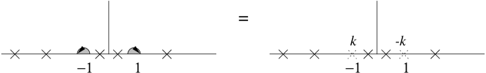
Figure 4: As $t\rightarrow\infty$, the annulus diagram can be approximated by the upper half-plane with momentum conserving tachyon insertions at $\lambda=\pm 1$. The leading-order disk amplitude is obtained by contracting the two tachyon insertions only with each other; contractions between external vertex operators and the insertions give rise to the first-order corrections.

Recall that the disk Green function on the upper half-plane is given by [4]

$${\mathcal{G}}^{\mu\nu}(\lambda_{i},\lambda_{j})=-\alpha^{\prime}G^{\mu\nu}\ln\left\lvert{\lambda_{i}-\lambda_{j}}\right\rvert^{2}+\frac{i}{2}\Theta^{\mu\nu}\epsilon(\lambda_{i}-\lambda_{j});$$ (27)

then the result of (26) can be easily written down. To keep our formula from becoming too long we will omit the modulus and coordinate integrations and unimportant prefactors, and write

$$S=(1-\lambda_{1}^{2})\left[\prod_{p<q=1}^{M}\left\lvert{\lambda_{p}-\lambda_{q}}\right\rvert^{2\alpha^{\prime}k_{p}\cdot k_{q}}\right]\,e^{\frac{i}{2}\sum_{i<j=1}^{N}(k_{i}\times k_{j})\epsilon(\tau_{ij})-{i\over 2}\sum_{r<s=N+1}^{M}(k_{r}\times k_{s})\epsilon(\tau_{rs})}\times I$$ (28)

with

$$\begin{split}I&=\int\frac{d^{d}k}{(2\pi)^{d}}e^{-2\pi t\alpha^{\prime}k^{2}}\exp\Bigl{[}-\text{\small$\sum_{p=1}^{M}$}2\alpha^{\prime}k\cdot(k_{p}\tau_{p})+i\text{\small$\sum_{i=1}^{N}$}k_{\mu}\Theta^{\mu\nu}k_{i\nu}\Bigr{]}\\ &=\sqrt{\det G}(8\pi^{2}\alpha^{\prime}t)^{-\frac{d}{2}}\exp\left[\frac{1}{8\pi\alpha^{\prime}t}\Bigl{(}\sum_{i=1}^{N}k_{i\mu}\Bigr{)}(\Theta G\Theta)^{\mu\nu}\Bigl{(}\sum_{j=1}^{N}k_{j\nu}\Bigr{)}\right]\\ &\quad\times\exp\left[\frac{\alpha^{\prime}}{2\pi t}\Bigl{(}\sum_{p=1}^{M}k_{p}\tau_{p}\Bigr{)}^{2}\right]e^{-\frac{i}{2\pi t}\sum_{i<j=1}^{N}(k_{i}\times k_{j})\tau_{ij}+\frac{i}{2\pi t}\sum_{r<s=N+1}^{M}(k_{r}\times k_{s})\tau_{rs}}\end{split}$$ (29)

It is can be checked that by combining equations (29) and (28) and restoring the prefactors in (28) we precisely recover (25). Since the oscillator parts of higher order operators always involve derivatives of the $X$, their contraction with external states will not result in any additional dependence on $\Theta$. So the contributions from oscillator modes follow exactly as in the $B=0$ case, while the new factors, (21) and the last exponential in (29), come from the open string zero modes.

2.2 Closed String Factorization

We examine the amplitude (19) in the closed string limit $t\rightarrow 0$, or $s\rightarrow\infty$. It is easy to see that (19) factorizes to closed string insertions on the disk in precisely the same manner as in the $B=0$ case. This follows since the $\Theta$-dependent factors are already factorized with respect to the two boundaries. Thanks to the factor (24), the closed string poles are indeed located according to the mass-shell condition in terms of the closed string metric. Here we shall demonstrate that the $\Theta$-dependent factors in the third line of (19) arise from the zero mode part of the closed string insertion. For this purpose it is again enough to look at the (closed string) tachyon insertion. The disk Green function on the unit circle in figure 1 is given by,

$${\cal G}^{\mu\nu}(\theta_{i},\theta_{j})=-\alpha^{\prime}G^{\mu\nu}\ln\left\lvert{2\sin\Bigl{(}\frac{\theta_{ij}}{2}\Bigr{)}}\right\rvert^{2}+\frac{i}{2}\Theta^{\mu\nu}\Bigl{[}\frac{\theta_{ij}}{\pi}-\epsilon(\theta_{ij})\Bigr{]}.$$ (30)

For pure open string amplitudes, the terms linear in $\theta_{ij}\equiv\theta_{i}-\theta_{j}$ in (30) cancel by momentum conservation. However when there is a closed string insertion the momentum conservation no longer causes it to vanish, but gives a contribution precisely as in the third line of (19).

Closed string factorization also gives an alternative derivation of the relation between closed and open string couplings. The relation was first derived in [4] by arguing the equivalence of the Born-Infeld actions expressed in terms of closed and open string parameters. Since numerical factors follow precisely as in $B=0$ case, here we shall only focus on the metric dependence. For tachyon insertion the factorization takes the form, (for convenience we take $d=26$)

$$S_{\text{annulus}}=\frac{1}{K_{c}}\,S_{D_{2}}(1,\dots,N,k)\,\frac{1}{k_{\mu}g^{\mu\nu}k_{\nu}-4}\,S_{D_{2}}(N+1,\dots,M,-k),$$ (31)

Figure 5: The closed string factorization of the annulus into two disks.

where $S_{D_{2}}$ is the disk amplitude with an extra tachyon insertion, and $K_{c}$ is the normalization of the tachyon two-point function on the sphere. Since

$$S_{\text{annulus}} \sim\sqrt{\det G}, S_{\text{disk}} \sim{1\over g_{o}^{2}}\sqrt{\det G}, K_{c} \sim\frac{1}{g_{c}^{2}}\sqrt{\det g},$$ (32)

from (31) and (32) we find that

$$g_{c}=2^{-18}\pi^{-25/2}{\alpha^{\prime}}^{-6}\,g_{o}^{2}\left(\frac{\det g}{\det G}\right)^{\frac{1}{4}}=2^{-18}\pi^{-25/2}{\alpha^{\prime}}^{-6}\,g_{o}^{2}\left(\frac{\det g}{\det(g+B)}\right)^{\frac{1}{2}}.$$ (33)

where the numerical factors are the same as in the $B=0$ case [37].

3 IR/UV and Stretched Strings

In the above we have shown that at the one-loop string theory level, the IR/UV factor (21) is a pure open string effect. It has a very different origin from the seemingly similar factor (24) in the closed string channel, which arises only after summing over an infinite number of open string oscillation modes. As we emphasized above, equation (21) is due solely to the zero modes. Thus we conclude, at least in bosonic open string theory, that the IR/UV factor (21) is not related to the appearance of the closed string modes of the string theory in which the noncommutative field theory is embedded.

Since we observed (21) occurring at the perturbative string theory level in precisely the same manner as it does in noncommutative field theories we might imagine that there is a simple explanation of (21) from string theory. After all, constant $B$ is a rather mild background from the string theory point of view, and we are supposed to know it very well. Indeed in the following we will present a very simple explanation.

If we denote

$$(\Delta x)^{\mu}=\Theta^{\mu\nu}p_{\nu}$$ (34)

and interpret it as a distance, then

$$(\Delta x)^{2}=-p_{\mu}(\Theta G\Theta)^{\mu\nu}p_{\nu}=G_{\mu\nu}(\Delta x)^{\mu}(\Delta x)^{\nu}$$ (35)

has the interpretation of a proper distance in terms of the open string metric, which indicates that there might be a stretched string interpretation of (21). This is supported by the fact that in the background $B$ field, $X$ has the following mode expansion:

$$X^{\mu}(\tau,\sigma)=x_{0}^{\mu}+2i\alpha^{\prime}p^{\mu}\tau+{1\over\pi}\Theta^{\mu\nu}p_{\nu}\,\sigma+(\alpha^{\prime})^{1\over 2}(\text{oscillators}).$$ (36)

Notice that with non-zero momentum there is an additional winding term proportional to $\Theta^{\mu\nu}p_{\nu}$. This has the consequence that, in addition to the standard oscillator piece the open string now has a finite constant stretched length,

$$X^{\mu}(\tau,\sigma=\pi)-X^{\mu}(\tau,\sigma=0)=\Theta^{\mu\nu}p_{\nu}+(\alpha^{\prime})^{1\over 2}({\rm oscillators})\ .$$ (37)

(a)
(b)

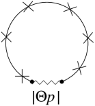
Figure 6: First quantized picture of a one loop graph in field theory for (a) $B=0$ and (b) $B\neq 0$.

Equation (37) is a beautiful manifestation of the UV/IR behavior of the system. When there is non-zero momentum flow between the two boundaries of the string, as is the case for non-planar diagrams, there is an induced stretched string. As an example, if we increase momentum in the $x^{1}$ direction by $\delta p_{1}$, the string grows longer in the $x^{2}$ direction by an amount $\left\lvert{\Theta^{21}\delta p_{1}}\right\rvert$. As we increase the momentum further the string stretches longer and longer. Since the first term in (37) has no $\alpha^{\prime}$ dependence, the stretched length $\Theta^{\mu\nu}p_{\nu}$ persists in the field theory limit. It will act as an effective short-distance cutoff. As $p\rightarrow 0$, the stretched string length decreases to zero and we start seeing the standard short-distance divergence again.

To understand the above picture more precisely, let us carefully go over the procedure of taking the $\alpha^{\prime}\rightarrow 0$ limit. Figure 2 represents a string world sheet with a coordinate width $\pi$ (and a space-time width in (37)) propagating through a proper time $2\pi t$. When $B=0$, as we take the field theory limit (22), the oscillation modes decouple and non-local effects caused by them in (37) also disappear and the worldsheet reduces to a circle of radius $\alpha^{\prime}t$—see figure 6a. The circle is the worldline of a finite number of loop particles in the first quantized picture. The $\alpha^{\prime}t\rightarrow 0$ limit amounts to shrinking the circle further to a point and is the usual short distance limit in field theory. In the second quantized picture $2\pi\alpha^{\prime}t$ may be identified as the Schwinger parameter $\tau$—

$${1\over k^{2}+m^{2}}=\int_{0}^{\infty}d\tau\,e^{-\tau(k^{2}+m^{2})}$$ (38)

—and $\tau\rightarrow 0$ corresponds to the limit of high momentum. Now turn on the $B$-field and allow a non-zero momentum to flow through the worldsheet as for non-planar scattering. Due to the presence of the first term in (37), the limit (22) no longer shrinks the world sheet to a circle, but instead to an arc of width $\left\lvert{\Theta^{\mu\nu}p_{\nu}}\right\rvert$—see figure 6b. After taking $\alpha^{\prime}t\rightarrow 0$, we are still left with a finite short-distance cutoff of $\left\lvert{\Theta^{\mu\nu}p_{\nu}}\right\rvert$. Note that the above interpretation fits very well with the way that (21) enters into the scattering amplitude (LABEL:ampop) ($\tau=2\pi\alpha^{\prime}t)$,

$$S=\int d\tau\,\tau^{-\frac{d}{2}-1}\,e^{-{\Delta x^{2}\over 4\tau}}\times(\cdots)\sim\int dt\,t^{-{d\over 2}-1}\,\exp\big{[}{1\over 8\pi\alpha^{\prime}t}p_{\mu}(\Theta G\Theta)^{\mu\nu}p_{\nu}\big{]}\times(\cdots)$$ (39)

The structure in equation (39) is the usual structure for a one-loop amplitude like figure 6b in the first-quantized approach to field theory; see e.g. ref. [42].

In the above discussion, the stretched strings appear to be rigid and non-dynamical; they merely cut open an otherwise closed particle loop. It is natural to ask whether this is due to our looking only at the one-loop level, for, after all, equation (36) is a tree-level expansion. The situation might change at higher genus; in particular, at the two-loop level, we will have vertices that are contracted only with internal lines. It is an interesting question whether the stretched string here is related to the “noncommutative QCD string” discussed in [43, 44, 5]. In [5] it was observed that the behaviour of higher genus diagrams suggests a string coupling of $g_{s}\sim 1/(E^{2}\Theta)$ which seems to be consistent with supergravity solutions [43, 44]. Similarly, we observe that equation (34) is reminiscent of the high energy proportionality between $x$ and $p$ [45] and thus suggests $\alpha^{\prime}_{\text{eff}}\sim\left\lvert{\Theta}\right\rvert$ (see also [46]).

4 Discussion and Conclusions

In this paper we have examined in detail the one-loop non-planar string amplitude for $M$ tachyons in bosonic open string theory with a $B$-field. We showed that the IR/UV mixing behavior of [5] can be understood as a pure open string effect in terms of the stretched strings. The mechanism is rather simple and general; in particular it simultaneously explains the various singularities (quadratic, logarithmic, etc.) of all operators (two-point, four-point, etc.).

In our approach, the IR singularities observed in [5] are not attributed to missing light degrees of freedom in the theory. They are rather a disguised reflection of the UV behaviour of the theory. The non-locality of the theory introduces a dynamical short-distance cutoff which is proportional to the external non-planar momentum $p$. The $p\rightarrow 0$ limit simply removes this cutoff and recovers the UV divergences.

This raises the question as to whether (bosonic) noncommutative theories are consistent. As already pointed out in [5], if we impose a cutoff $\Lambda=1/\epsilon$ into the theory then for $(\Delta x\equiv\Theta p)<\epsilon$ the limit of taking $\Lambda\rightarrow\infty$ is not well-defined since there is a crossover between $\Delta x$ and $\epsilon$. For example, if we consider a noncommutative scalar $\Phi^{3}$ theory in six dimensions, or any other theory that is renormalizable for $\Theta=0$, embedded in a string theory, then the natural cutoff of the theory is $\epsilon=(\alpha^{\prime})^{1/2}$. Let us first assume $\Theta>\alpha^{\prime}$, where here and in the following, by $\Theta$ we mean, roughly, the magnitude of a typical eigenvalue. There are now two ways of “detecting” the effects of the massive string modes. One is obvious; they are excited at high energies of order $(\alpha^{\prime})^{-1/2}$. The other is to go to very low energies of order $(\alpha^{\prime})^{1/2}/\Theta$. More explicitly, inside the energy region

$$(\alpha^{\prime})^{1/2}/\Theta<p<(\alpha^{\prime})^{-1/2},$$ (region I)

the one-loop effective action has the heuristic form

$$\Gamma(k)=\Gamma_{\text{planar}}(k,(\alpha^{\prime})^{1/2})+\Gamma_{\text{non-planar}}(k,\Theta p)$$ (40)

where $k$ denotes generic external momenta, $p$ non-planar momenta, and the second variable denotes the cutoff. The non-planar amplitudes are finite; planar diagrams can be renormalized in the usual sense; and the $\alpha^{\prime}\rightarrow 0$ limit can be consistently defined. However as we reach the region of small momenta,

$$p<(\alpha^{\prime})^{1/2}/\Theta,$$ (region II)

the effective action becomes

$$\Gamma(k)=\Gamma_{\text{planar}}(k,(\alpha^{\prime})^{1/2})+\Gamma_{\text{non-planar}}(k,(\alpha^{\prime})^{1/2})$$ (41)

i.e. $\alpha^{\prime}$ effects will take over below energy scales of order $(\alpha^{\prime})^{1/2}/\Theta$. This crossover can be seen explicitly in equation (36); below this scale the oscillator terms become important compared to the $\Theta^{\mu\nu}p_{\nu}\sigma$ term. Now, unlike for ordinary field theories, it is no longer consistent to take the $\alpha^{\prime}\rightarrow 0$ limit since the behaviour of the full theory, when $(\alpha^{\prime})^{1/2}$ becomes smaller than $\Theta p$, is such that the effective theory of equation (41) is no longer valid, but rather we go over to the region I behaviour (40). We should caution that this discussion is only at the one-loop level. At the two-loop level the loop integration over $p$ will result in divergent diagrams, a reflection of the one-loop IR singularities.

Thus it appears that although naïvely—as we have seen in section 2—the massive modes seem to decouple in the amplitude in the limit (22), in fact the oscillators are quite important. What is surprising is that they preclude a proper Wilsonian description at low non-planar momentum! Only if we keep $\Theta<\alpha^{\prime}$ as $\alpha^{\prime}\rightarrow 0$ do we recover Wilsonian field theory, but it is then a commutative field theory. Thus, for a noncommutative theory, we see here an intricate interplay between two scales $\Theta$ and $\alpha^{\prime}$.

This is not to suggest that we cannot add new fields, along the lines of [5, 12], to reinterprete the IR singularities. Rather, we point out that this interpretation of the singularities is not one that arises naturally out of bosonic string theory.

- [1] A. Connes, M. R. Douglas and A. Schwarz, Noncommutative geometry and matrix theory: Compactification on tori, J. High Energy Phys. 02 (1998) 003; [hep-th/9711162].
- [2] M. R. Douglas and C. Hull, D-branes and the Noncommutative Torus, J. High Energy Phys. 02 (1998) 008; [hep-th/9711165].
- [3] M. Li, Strings from IIB Matrices, Phys. Lett. B 499 (1997) 149–158; [hep-th/9612222].
- [4] N. Seiberg and E. Witten, String theory and noncommutative geometry, J. High Energy Phys. 09 (1999) 032; [hep-th/9908142].
- [5] S. Minwalla, M. Van Raamsdonk and N. Seiberg, Noncommutative Perturbative Dynamics, PUPT-1905, IASSNS-HEP-99-112, hep-th/9912072.
- [6] T. Filk, Divergences in a Field Theory on Quantum Space, Phys. Lett. B 376 (1996) 53.
- [7] M. M. Sheikh-Jabbari, Open Strings in a B-field Background as Electric Dipoles, Phys. Lett. B 455 (1999) 129–134; [hep-th/9901080].
- [8] D. Bigatti and L. Susskind, Magnetic Fields, Branes and Noncommutative Geometry, SU-ITP 99/39, KUL-TF 99/30, hep-th/9908056.
- [9] Z. Yin, A Note on Space Noncommutativity, Phys. Lett. B 466 (1999) 234–238; [hep-th/9908152].
- [10] A. Matusis, L. Susskind and N. Toumbas, The IR/UV Connection in the Non-Commutative Gauge Theories, SU-ITP 00-07, hep-th/0002075.
- [11] R. Gopakumar, S. Minwalla and A. Strominger, Noncommutative Solitons, hep-th/0003160.
- [12] M. Van Raamsdonk and N. Seiberg, Comments on Noncommutative Perturbative Dynamics, IASSNS-HEP-00/13, PUPT-1920, hep-th/0002186.
- [13] M.Hayakawa, Perturbative Analysis on Infrared Aspects of Noncommutative QED on , hep-th/9912094; Perturbative Analysis on Infrared and Ultraviolet Aspects of Noncommutative QED on , hep-th/9912167.
- [14] H. Grosse, T. Krajewski and R. Wulkenhaar, Renormalization of Noncommutative Yang-Mills Theories: A Simple Example, UWThPh-2000-9, SISSA/6/2000/FM, hep-th/0001182.
- [15] I. Y. Aref’eva, D. M. Belov and A. S. Koshelev, A Note on UV/IR for Noncommutative Complex Scalar Field, SMI-5-00, hep-th/0001215.
- [16] I. Ya. Aref’eva, D. M. Belov, A. S. Koshelev and O. A. Rytchkov, UV/IR Mixing for Noncommutative Complex Scalar Field Theory, II (Interaction with Gauge Fields), SMI-6-00, hep-th/0003176.
- [17] W. Fischler, E. Gorbatov, A. Kashani-Poor, S. Paban, P. Pouliot and J. Gomis, Evidence for Winding States in Noncommutative Quantum Field Theory, UTTG-03-00, hep-th/0002067.
- [18] W. Fischler, E. Gorbatov, A. Kashani-Poor, R. McNees, S. Paban and P. Pouliot, The Interplay Between and T, UTTG-05-00, hep-th/0003216.
- [19] C-S. Chu, Induced Chern Simons and WZW Action in Noncommutative Spacetime, NEIP-00-004, hep-th/0003007.
- [20] B.A. Campbell and K. Kaminsky, Noncommutative Field Theory and Spontaneous Symmetry Breaking, Alberta Thy 03-00, hep-th/0003137.
- [21] A. Rajaraman and M. Rozali, Noncommutative Gauge Theory, Divergences and Closed Strings, RUNHETC-2000-10, hep-th/0003227.
- [22] Y.-K. E. Cheung and M. Krogh, Noncommutative Geometry From 0-Branes in a Background B Field, Nucl. Phys. B 528 (1998) 185–196; [hep-th/9803031].
- [23] F. Ardalan, H. Arfaei and M.M. Sheikh-Jabbari, Noncommutative Geometry from Strings and Branes, J. High Energy Phys. 02 (1999) 016; [hep-th/9810072].
- [24] C.-S. Chu and P.-M. Ho, Noncommutative Open String And D-Brane, Nucl. Phys. B 550 (1999) 151–168, [hep-th/9812219]; Constrained Quantization of Open String in Background B Field and Noncommutative D-brane, NEIP-99-011, hep-th/9906192.
- [25] V. Schomerus, D-Branes and Deformation Quantization, J. High Energy Phys. 06 (1999) 030; [hep-th/9903205].
- [26] H. Aoki, N. Ishibashi, S. Iso, H. Kawai, Y. Kitazawa, T. Tada, Noncommutative Yang-Mills in IIB Matrix Model, KEK-TH-637, KUNS-1595, hep-th/9908141; N. Ishibashi, S. Iso, H. Kawai, Y. Kitazawa, Wilson Loops in Noncommutative Yang Mills, KEK-TH-649, KUNS-1608, hep-th/9910004.
- [27] S. Iso, H. Kawai and Y. Kitazawa, Bi-local Fields in Noncommutative Field Theory, KEK-TH-669, KUNS-1628, hep-th/0001027.
- [28] J. Ambjorn, Y.M. Makeenko, J. Nishimura and R.J. Szabo, Finite N Matrix Models of Noncommutative Gauge Theory, J. High Energy Phys. 11 (1999) 029; [hep-th/9911041].
- [29] J. Ambjorn, Y.M. Makeenko, J. Nishimura and R.J. Szabo, Nonperturbative Dynamics of Noncommutative Gauge Theory, NBI-HE-00-08, ITEP-TH-10/00, hep-th/0002158.
- [30] O. Andreev and H. Dorn, Diagrams of Noncommutative Phi-Three Theory from String Theory, HU Berlin-EP-00/19, hep-th/0003113
- [31] Y. Kiem and S. Lee, UV/IR Mixing in Noncommutative Field Theory via Open String Loops, KIAS-P00013, hep-th/0003145.
- [32] A. Bilal, C.-S. Chu and R. Russo, String Theory and Noncommutative Field Theories at One Loop, NEIP-00-008, hep-th/0003180.
- [33] J. Gomis, M. Kleban, T. Mehen, M. Rangamani and S. Shenker, Noncommutative Gauge Dynamics From The String Worldsheet, CALT-68-2267, CITUSC/00-016, SU-ITP-00-11, hep-th/0003215.
- [34] E.S. Fradkin and A.A. Tseytlin, Nonlinear Electrodynamics from Quantized Strings, Phys. Lett. B 163 (1985) 123–130.
- [35] A. Abouelsaood, C.G. Callan, C.R. Nappi and S.A. Yost, Open Strings in Background Gauge Fields, Nucl. Phys. B 280 [FS 18] (1987) 599–624.
- [36] C.G. Callan, C. Lovelace, C.R. Nappi and S.A. Yost, String Loop Corrections to Beta Functions, Nucl. Phys. B 288 (1987) 525–550.
- [37] J. Polchinski, String Theory: Volume I, An Introduction to the Bosonic String, Cambridge University Press, Cambridge, 1998.
- [38] P. Di Vecchia, L. Magnea, A. Lerda, R. Russo and R. Marotta, String Techniques for the Calculation of Renormalization Constants in Field Theory, Nucl. Phys. B 469 (1996) 235–286; [hep-th/9601143].
- [39] R.R. Metsaev and A.A. Tseytlin, On Loop Corrections to String Theory Effective Actions, Nucl. Phys. B 298 (1988) 109–132.
- [40] M.B. Green, J.H. Schwarz and E. Witten, Superstring Theory, Cambridge University Press, Cambridge, 1987, Chapter 8.
- [41] J. Polchinski, Factorization of Bosonic String Amplitudes, Nucl. Phys. B 307 (1988) 61–92.
- [42] A. Polyakov, Gauge Fields and Strings, Harwood Academic Publishers, London, 1987, Chapter 9.
- [43] A. Hashimoto and N. Itzhaki, Non-Commutative Yang-Mills and the AdS/CFT Correspondence, Phys. Lett. B 465 (1999) 142–147; [hep-th/9907166].
- [44] J.M. Maldacena and J.G. Russo, Large N Limit of Non-Commutative Gauge Theories, J. High Energy Phys. 09 (1999) 025; [hep-th/9908134].
- [45] D. J. Gross and P. F. Mende, The High-Energy Behavior Of String Scattering Amplitudes, Phys. Lett. B 197 (1987) 129–134; String Theory Beyond The Planck Scale, Nucl. Phys. B 303 (1988) 407–454.
- [46] N. Ishibashi, S. Iso, H. Kawai and Y. Kitazawa, String Scale in Noncommutative Yang-Mills, KEK-TH-683, KUNS-1655, hep-th/0004038.