OUTP-00-06P, UPR-880T, HUB-EP-00/10
hep-th/0003256
Heterotic M–Theory Cosmology in Four and Five Dimensions

We study rolling radii solutions in the context of the four– and five–dimensional effective actions of heterotic M–theory. For the standard four–dimensional solutions with varying dilaton and T–modulus, we find approximate five–dimensional counterparts. These are new, generically non–separating solutions corresponding to a pair of five–dimensional domain walls evolving in time. Loop corrections in the four–dimensional theory are described by certain excitations of fields in the fifth dimension. We point out that the two exact separable solutions previously discovered are precisely the special cases for which the loop corrections are time–independent. Generically, loop corrections vary with time. Moreover, for a subset of solutions they increase in time, evolving into complicated, non-separating solutions. In this paper we compute these solutions to leading, non-trivial order. Using the equations for the induced brane metric, we present a general argument showing that the accelerating backgrounds of this type cannot evolve smoothly into decelerating backgrounds.

1 Introduction

Among the simplest cosmological solutions of string theory are the so called rolling radii solutions [1]. They are characterized by a kinetic–energy driven evolution of the universe. These fundamental solutions of string cosmology provide superinflating cosmological backgrounds as well as subluminally expanding backgrounds of Friedmann–Robertson–Walker type [2, 3, 4].

In the present paper, we will analyze and discuss rolling radii solutions from the perspective of the string theory/M–theory relation. In particular, we will discuss how a superinflating phase in string cosmology is embedded into an M–theory context. This will be done within the framework of the four–dimensional $N=1$ effective action of the $E_{8}\times E_{8}$ heterotic string theory and the underlying five–dimensional effective action of heterotic M–theory [5, 6, 7], obtained from 11–dimensional Hořava–Witten theory [8, 9, 10, 11] by reduction on a Calabi–Yau three–fold with non–vanishing G–flux. This five–dimensional action constitutes an M–theory realization of a “brane–world”. In precisely this context, we will analyze rolling radii solutions and the role the fifth dimension plays in the cosmological evolution they describe. In particular, we will present a new class of non–separating five–dimensional solutions that represents the direct generalization of the well–known four–dimensional rolling radii solutions to heterotic M–theory.

Cosmological rolling radii solutions of M–theory related to branes have first been obtained in ref. [12, 13, 14, 15]. The first cosmological solutions of five–dimensional heterotic M–theory have been found in ref. [16]. These latter solutions are generalized rolling radii solutions with an inhomogeneous fifth dimension. Subsequently, further examples of cosmological solutions to five–dimensional heterotic M–theory have been presented [17]–[21]. One purpose of this paper is to clarify the role of the solutions given in ref. [16] in the present context. Potential–driven inflation and its relation to five–dimensional heterotic M–theory has been first analyzed in ref. [22]. The present paper is somewhat complementary to this work in that it addresses similar questions, however for the case of kinetic–energy driven inflation. Recently, there is also considerable activity, see for example [18]–[30], exploring other cosmological aspects of five–dimensional brane–world theories. M–theory rolling radii cosmology based on vacua with a large number of supersymmetries has been investigated in ref. [31]. In the present paper, we consider a related situation but focus on vacua with the “phenomenological” value of $N=1$ supersymmetry in four dimensions. While this situation is of course physically favorable, we have much less control over quantum effects than in the cases analyzed in ref. [31]. In this paper, we focus on the effect of string loop corrections in four dimensions while, for simplicity, we work at lowest order in $\alpha^{\prime}$. Also, we will not attempt to include non–perturbative effects such as brane instantons. Clearly, it would be interesting to extend the analysis presented in this paper to include some of these effects.

Let us outline the paper and summarize its main results. To set the stage, we first review the relation between the four– and five–dimensional effective actions of heterotic M–theory as presented in ref. [5, 22]. In particular, we show how the relevant four–dimensional fields, that is, the four–dimensional metric $g_{4}$, the dilaton $S_{R}$ and the T–modulus $T_{R}$ arise as moduli of the five–dimensional three–brane vacuum solution. We also review the correspondence between excitations of the bulk fields in the fifth dimension and string loop corrections to the four–dimensional effective action. Correspondingly, the strong coupling expansion parameter $\epsilon\sim T_{R}/S_{R}$ can be interpreted as measuring the strength of those bulk excitations as well as the size of the loop corrections. Then, we start with the standard class of four–dimensional rolling radii solutions where we allow the scale factor of the three–dimensional universe, the dilaton and the T–modulus to vary in time. Discarding trivial integration constants, those solutions form a one–parameter set. We then show, using the correspondence between the four– and five–dimensional effective theories, how this complete set can be “lifted up” to approximate solutions of the five–dimensional effective action. Due to the potentials present in the five–dimensional theory, these solutions depend on the fifth coordinate as well as on time and are generically non–separating. They constitute new, non–trivial solution of the five–dimensional effective action of heterotic M–theory that generalize the familiar four–dimensional rolling radii solutions. More specifically, they correspond to a pair of domain wall three–branes with rolling radii. In addition to the overall scaling that is familiar from four–dimensional rolling radii solutions, there is another non–trivial feature of those solutions not visible from a four–dimensional viewpoint. The size of the domain wall bulk excitations (and hence the parameter $\epsilon$) is generically varying in time. It is this time variation of the internal domain wall structure that makes the solutions non–separating and, hence, non–trivial.

We can classify the solutions according to the time–behavior of $\epsilon$. It turns out that there are exactly two solutions (out of the one–parameter set) for which $\epsilon=$ const. In those two cases, one can find exact separable solutions which are precisely the ones that have been given in ref. [16]. For all other cases, $\epsilon$ varies in time and the corresponding exact solution must be non–separating. As a result, the separable solutions are exactly the ones for which loop corrections (or equivalently five–dimensional bulk excitations) are independent of time and are, hence, under control at all stages of the evolution. The remaining solutions with non–constant $\epsilon$ split into two (one–parameter) subsets, one with increasing $\epsilon$ and the other with decreasing $\epsilon$ in the negative–time branch. Particularly, the former case of increasing $\epsilon$ is interesting. In this case, an effectively four–dimensional solution is subject to increasing loop corrections that can be described by bulk excitations in the five–dimensional theory. When $\epsilon$ is of order one, the approximate five–dimensional solution is no longer valid and the subsequent evolution is described by a more complicated non–separating background. In particular, then, the time evolution and the dependence of the fields on the additional dimension are entangled in a complicated way. An interesting question is whether this might help to avoid the curvature singularity at the end of the negative–time branch. Unfortunately, no exact analytic solution is known to us in this non–separating case. However, we present an argument, based on the evolution equations for the induced fields on the boundaries, that a branch change does not occur, even at large values of $\epsilon$.

2 Heterotic M-theory in four and five dimensions

A popular starting point for string cosmology is the lowest–order four–dimensional effective action

$$S_{4}=-\frac{1}{16\pi G_{N}}\int_{M_{4}}\sqrt{-g_{4}}e^{-\phi_{4}}\left[R_{4}-\partial_{\mu}\phi_{4}\partial^{\mu}\phi_{4}+\frac{3}{2}\partial_{\mu}\beta_{4}\partial^{\mu}\beta_{4}+\mbox{(matter field terms)}\right]$$ (2.1)

written in the string frame. This action can be viewed as a universal effective action for $N=1$ compactifications (on Calabi–Yau three–folds) of weakly coupled $E_{8}\times E_{8}$ heterotic string theory. In fact, the field content has been truncated to the fields essential for a discussion of string cosmology, that is, gravity and the two universal moduli $\phi_{4}$ and $\beta_{4}$. In terms of the dilaton $S$ and the conventional T–modulus $T$, we can express those fields as

$$S_{R}=e^{\phi_{4}}\;,\qquad T_{R}=e^{\beta_{4}}\;.$$ (2.2)

Here $S_{R}$ and $T_{R}$ denote the real parts of the bosonic component in the respective $N=1$ superfields.

Given the origin of the above action, it should be possible to relate it to the strong coupling limit of the $E_{8}\times E_{8}$ string theory [8, 9, 10, 11] in its effective formulation via heterotic M–theory, that is, M–theory on the orbifold $S^{1}/Z_{2}$. In fact, the simplest and perhaps conceptually most interesting connection is the one to five–dimensional heterotic M–theory [5, 7]. Let us, therefore, discuss the simplest version of this five–dimensional theory briefly. For more details, we refer the reader to ref. [5, 7, 22].

This theory is obtained from its 11–dimensional counterpart by a reduction on a Calabi–Yau three–fold with a non–vanishing G–flux. Then the five–dimensional space–time has the structure $M_{5}=S^{1}/Z_{2}\times M_{4}$ where $M_{4}$ is a smooth $3+1$ dimensional space–time. We will use coordinates $x^{\alpha}$ with indices $\alpha,\beta,\gamma,\cdots=0,1,2,3,5$ for the full five–dimensional space–time and coordinates $x^{\mu}$ with $\mu,\nu,\rho,\cdots=0,1,2,3$ for $M_{4}$. Furthermore, the $S^{1}$ coordinate $y\equiv x^{5}$ is restricted to the range $y\in[-\pi\rho,\pi\rho]$ where $\rho$ is the radius of the orbicircle. In these coordinates, the action of the $Z_{2}$ symmetry on $S^{1}$ is defined as $y\rightarrow-y$. This leads to two four–dimensional fixed planes $M_{4}^{1}$ and $M_{4}^{2}$ at $y=0$ and $y=\pi\rho$, respectively. The theory on this space–time constitutes a five–dimensional $N=1$ gauged supergravity theory in the bulk coupled to two four–dimensional $N=1$ theories on $M_{4}^{1}$ and $M_{4}^{2}$. A simple version [22] of this theory is given by

$$S_{5}=-\frac{1}{2\kappa_{5}^{2}}\left\{\int_{M_{5}}\sqrt{-g}\left[R+\frac{1}{2}\partial_{\alpha}\phi\partial^{\alpha}\phi+\frac{1}{3}v^{2}e^{-2\phi}\right]\right.\\ +\left.\sum_{n=1}^{2}\int_{M_{4}^{n}}\sqrt{-g}\left[\mp 2\sqrt{2}ve^{-\phi}+\mbox{(matter field terms)}\right]\right\}\;.$$ (2.3)

Here $\kappa_{5}$ is the five–dimensional Newton constant, $v$ is a constant that depends on internal instanton numbers and $\phi$ is the five–dimensional dilaton field. Its geometrical interpretation is to measure the size of the internal Calabi–Yau space such that its volume is proportional to $\exp(\phi)$. In the same spirit as for the four–dimensional action above, we have confined ourselves to the field content that is essential for our cosmological discussion. The above action constitutes an explicit realization of a five–dimensional brane–world in the context of M–theory, as was first realized in ref. [5].

How precisely are the effective actions (2.1) and (2.3) related? This has been worked out in ref. [5, 7] and we would like to briefly review some of the results. Note that for $v\neq 0$, the action (2.3) does not admit flat five–dimensional space–time as a solution. Instead, its “vacuum” is a pair of domain walls or three–branes specified by the exact solution [5]

$$ds_{5}^{2}=a_{0}^{2}Hdx^{\mu}dx^{\nu}\eta_{\mu\nu}+b_{0}^{2}H^{4}dy^{2}\;,\qquad e^{\phi}=b_{0}H^{3}$$ (2.4)

with harmonic function $H=H(y)$ given by

$$H=c_{0}+\frac{1}{3}\epsilon_{0}h(y)\;,\qquad h(y)=\frac{|y|}{\pi\rho}-\frac{1}{2}$$ (2.5)

where $\epsilon_{0}=\sqrt{2}\pi\rho v$ and $a_{0}$, $b_{0}$ and $c_{0}$ are arbitrary constants. This solution preserves $3+1$–dimensional Poincaré invariance and represents a BPS solution of the five–dimensional supergravity theory described by action (2.3). Hence, a reduction of the five–dimensional theory on this three–brane solution to four dimensions leads to a generally covariant $N=1$ supersymmetric theory. This theory is, of course, the four–dimensional effective action of the $E_{8}\times E_{8}$ string whose universal part has been given in eq. (2.1) above. Phrased in a different way, the four–dimensional theory provides an effective description for the moduli of the domain wall solution. To make this explicit, define constants $\beta_{4}$ and $\phi_{4}$ by

$$b_{0}=e^{3\beta_{4}-2\phi_{4}}\;,\qquad c_{0}=e^{\phi_{4}-\beta_{4}}$$ (2.6)

as well as a four–dimensional metric $g_{4\mu\nu}$ by

$$g_{4\mu\nu}=a_{0}^{2}e^{2\phi_{4}}\eta_{\mu\nu}\;.$$ (2.7)

Note that we can perform a general linear transformation on the coordinates $x^{\mu}$ in the solution (2.4). This converts $\eta_{\mu\nu}$ and, hence, $g_{4\mu\nu}$ into an arbitrary four–dimensional metric. It follows that, to leading order in $\epsilon_{0}$ the solution takes the form

$$ds_{5}^{2}=\left(1+\frac{1}{3}\epsilon h\right)e^{-\beta_{4}-\phi_{4}}dx^{\mu}dx^{\nu}g_{4\mu\nu}+\left(1+\frac{4}{3}\epsilon h\right)e^{2\beta_{4}}dy^{2}\;,\qquad\phi=\phi_{4}+\epsilon h$$ (2.8)

where

$$\epsilon=\epsilon_{0}e^{\beta_{4}-\phi_{4}}\;.$$ (2.9)

and $h=h(y)$ is as defined above. The metric $g_{4\mu\nu}$ can be interpreted as the four–dimensional string–frame metric. The moduli $\phi_{4}$ and $\beta_{4}$ measure the internal Calabi–Yau volume $V$ and the orbifold size $R$, averaged over the orbifold coordinate . The metric and these moduli can now be promoted to four–dimensional fields depending on $x^{\mu}$. As discussed in ref. [5, 7], the low–energy dynamics of these fields can be obtained by reducing the five–dimensional action (2.3) using the ansatz (2.8). The resulting dynamics is precisely described by action (2.1). Note that this action depends on all three moduli $a_{0}$, $b_{0}$ and $c_{0}$ of the exact three–brane solution. Modulus $a_{0}$ is related to the scale factor in the four–dimensional metric $g_{4\mu\nu}$, whereas $b_{0}$ and $c_{0}$ enter the effective four–dimensional action through

$$S_{R}=b_{0}c_{0}^{3}\;,\qquad T_{R}=b_{0}c_{0}^{2}\;,$$ (2.10)

where we have used (2.2) and (2.6). This establishes a direct relationship between five–dimensional solutions based on the three–brane (2.8) and solutions of the four–dimensional effective action (2.1) for the moduli. Hence, via eq. (2.8), any cosmological solution of the four–dimensional theory immediately implies a (approximate) cosmological solution in five–dimensions, and vice versa.

As is apparent from the four–dimensional action (2.1), we are working to lowest order in $\alpha^{\prime}$. Correspondingly, we have neglected higher derivative terms in the five–dimensional action (2.3) as well. For example, to lowest order we expect $R^{2}$ and $R^{4}$ terms in the bulk originating from the $R^{4}$ term in M–theory [32] as well as $R^{2}$ terms on the boundary [33]. Although it would be interesting to include those corrections, particularly from a five–dimensional viewpoint, for the purpose of this paper we will focus on situations where higher–derivative corrections are still small.

There is another requirement for the four–dimensional effective description to be valid. We have used a linearized approximation in

$$\epsilon=\epsilon_{0}e^{\beta_{4}-\phi_{4}}\sim\frac{R}{V}\sim\frac{T_{R}}{S_{R}}$$ (2.11)

and, hence, $\epsilon$ should be smaller than one for the action (2.1) to be sensible. What is the meaning of this last condition? Eq. (2.11) leads us to three different interpretations of the so–called strong coupling expansion parameter $\epsilon$. First, $\epsilon$ measures the excitation of bulk gravity in the domain wall solution (2.4) due to the bulk and boundary potentials in the five–dimensional action. That is, $\epsilon$ measures the variation of the metric (and the dilaton) as one moves across the orbifold. Second, it measures the relative size $R/V$ of the orbifold and the internal Calabi–Yau space. And third, it measures the relative size of string–loop corrections to the four–dimensional effective action which is indeed proportional to $T_{R}/S_{R}$. The relation between loop corrections and bulk gravity is not accidental. One can verify that the one loop corrections to the four–dimensional effective action are in fact generated by the non–trivial structure of the domain wall solution [7]. Hence, the linear approximation in $\epsilon$ implies that we are considering a four–dimensional one–loop effective action or, equivalently, five–dimensional bulk excitations that are well approximated by linearized gravity. In the following, we will use the term “bulk excitations” to mean this non–trivial orbifold dependence induced by the potentials in the five–dimensional theory and related to loop corrections. Note that, due to the $R^{2}$ corrections on the boundaries mentioned above, higher–derivative corrections will also induce a non–trivial orbifold dependence whenever those corrections become relevant. It would be interesting to include those higher derivative terms, specifically the boundary $R^{2}$ terms, in the analysis. A related four–dimensional analysis with $R^{2}$ terms has been performed in ref. [34]. Higher curvature terms in five dimensions have been considered in ref. [35], however the boundary $R^{2}$ terms were not included in the analysis of this paper. As stated above, in this paper, we confine ourselves to the lowest order in $\alpha^{\prime}$.

Does the five–dimensional action (2.3) and, correspondingly, its exact domain–wall solution (2.4) encode higher loop–effects as well? Certainly it contains information beyond the one–loop level, since the bulk potential in eq. (2.3) which is uniquely fixed by five–dimensional supersymmetry is of the order $v^{2}\sim\epsilon^{2}$. However, higher–order corrections to the five–dimensional action cannot be excluded. Therefore, while one expects higher loop corrections to be described by bulk gravity effects and an action of the type above, there might be modifications of the concrete form (2.3) at higher order.

3 Cosmological solutions

Based on the above correspondence between the four– and five–dimensional theories we would now like to discuss the simplest type of cosmological solutions, namely rolling radii solutions. These solutions are characterized by an evolution of the universe driven by kinetic energy and they provide superinflating as well as subluminally expanding cosmological string backgrounds [2]. First, we would like to review those solutions in the four–dimensional context. Then we present new five–dimensional solutions that constitute the generalization of rolling radii solutions to heterotic M–theory. Furthermore, we discuss their relation to the known four–dimensional solutions.

Let us first recall the conventional picture that arises in four dimensions. We choose a four–dimensional metric of Friedmann–Robertson–Walker type with flat spatial sections and scale factor $\alpha_{4}=\alpha_{4}(t_{4})$, that is,

$$ds_{4}^{2}=g_{4\mu\nu}dx^{\mu}dx^{\nu}=-dt_{4}^{2}+e^{2\alpha_{4}}d{\bf x}^{2}\;.$$ (3.1)

Accordingly, the other two fields are taken to be functions of time only, that is, $\beta_{4}=\beta_{4}(t_{4})$ and $\phi_{4}=\phi_{4}(t_{4})$. Then the general solution of the four–dimensional action (2.1) is of the form

$$\alpha_{4}=p_{4\alpha}\ln|t_{4}|+\bar{\alpha}_{4}\;,\qquad\beta_{4}=p_{4\beta}\ln|t_{4}|+\bar{\beta}_{4}\;,\qquad\phi_{4}=p_{4\phi}\ln|t_{4}|+\bar{\phi}_{4}\;,$$ (3.2)

where $\bar{\alpha}_{4}$, $\bar{\phi}_{4}$ and $\bar{\beta}_{4}$ are arbitrary constants. The expansion powers ${\bf p}_{4}\equiv(p_{4\alpha},p_{4\beta},p_{4\phi})$ are subject to the two constraints

$$3p_{4\alpha}-p_{4\phi}=1\;,\qquad 9p_{4\beta}^{2}+4p_{4\phi}+2p_{4\phi}^{2}=4\;.$$ (3.3)

Apart from trivial integration constants such as $\bar{\alpha}_{4}$, $\bar{\beta}_{4}$ and $\bar{\phi}_{4}$, we therefore have a one–parameter family of solutions specified by the solutions to eq. (3.3). Generically, the scale factor of the universe as well as both moduli fields evolve in time. As usual, for each set of allowed expansion coefficients, we have a solution in the negative–time branch, that is, for $t_{4}<0$ and a solution in the positive–time branch, that is for $t_{4}>0$. As stands, the former evolves into a future curvature singularity while the latter arises from a past curvature singularity. Frequently, for the discussion of superinflating cosmology, specific solutions are chosen from the set specified by (3.3). These specific solutions are characterized by a constant T–modulus and, hence, by the expansion coefficients

$${\bf p}_{4}^{(T)}=\left(\pm\frac{1}{\sqrt{3}},0,\pm\sqrt{3}-1\right)\;.$$ (3.4)

As discussed in the previous section, the quantity $\epsilon$, defined in eq. (2.11), is of particular importance in our context as it measures the size of the four–dimensional loop corrections as well as the five–dimensional gravitational bulk excitations. Going back to the general class of solutions, we have from eq. (2.11) and (3.2) that

$$\epsilon\sim|t_{4}|^{p_{4\beta}-p_{4\phi}}\;.$$ (3.5)

Generally, therefore, $\epsilon$ will be time–dependent. However, we can ask if there are special solutions in the above set for which $p_{4\beta}=p_{4\phi}$ and, hence, $\epsilon$ is constant. Such solutions indeed exist and are characterized by the expansion powers

$${\bf p}_{4}^{(\epsilon)}=\left(\frac{3}{11}\left(1\pm\frac{4}{3\sqrt{3}}\right),\frac{2}{11}\left(-1\pm 2\sqrt{3}\right),\frac{2}{11}\left(-1\pm 2\sqrt{3}\right)\right)\;.$$ (3.6)

While, in the following, we will work with the general set of solutions, we will comment on these special cases where appropriate. After this review of the four–dimensional solutions, let us now move on to the five–dimensional case.

Our goal is to specify the five–dimensional origin of the above rolling radii solutions. That is, we would like to find the solutions of the five–dimensional theory (2.3) that, in the small–momentum limit, reduce to the four–dimensional rolling radii solutions. From the action (2.3), it is clear that those solutions, in addition to time, must depend on the orbifold coordinate $y$, as long as the constant $v$ is non–zero. In fact, while models with $v=0$ exist [36], generically $v$ is non–vanishing. As a consequence, exact cosmological solutions of the action (2.3) are not easy to find. The first example has been given in ref. [16] using separation of variables and we will come back to this example later on. Some generalizations, also based on separation of variables, including those with curved three–dimensional spatial section have been presented subsequently [17]. Exact, non–separating solutions have been found for a related action set up to describe the somewhat different physical situation of potential–driven inflation within M–theory [22]. However, exact non–separating solutions for the action (2.3) are hard to find and not a single example is known to date. In this paper, we will, therefore, content ourselves with giving approximate non–separable solutions. Such solutions can be obtained by “lifting up” the four–dimensional rolling radii solutions to five dimensions using the correspondence (2.8) between the four– and five–dimensional theories. Concretely, by inserting (3.1) and (3.2) into eq. (2.8), we obtain as the approximate solution of the five–dimensional action (2.3)

$$ds_{5}^{2}=(1+\epsilon h/3)\left(-dt_{5}^{2}+e^{2\alpha_{5}}d{\bf x}^{2}\right)+(1+4\epsilon h/3)e^{2\beta_{5}}dy^{2}\;,\qquad e^{\phi}=e^{\phi_{5}}(1+\epsilon h)$$ (3.7)

where we have introduced the five–dimensional “comoving” time $t_{5}$ by

$$dt_{5}^{2}=e^{-\beta_{5}-\phi_{5}}dt_{4}^{2}\;.$$ (3.8)

The five–dimensional scale factors $\alpha_{5}$, $\beta_{5}$ and $\phi_{5}$ show a power–law behavior

$$\alpha_{5}=p_{5\alpha}\ln|t_{5}|+\bar{\alpha}_{5}\;,\qquad\beta_{5}=p_{5\beta}\ln|t_{5}|+\bar{\beta}_{5}\;,\qquad\phi_{5}=p_{5\phi}\ln|t_{5}|+\bar{\phi}_{5}\;,$$ (3.9)

similar to the one in four dimensions. The expansion coefficients ${\bf p}_{5}=(p_{5\alpha},p_{5\beta},p_{5\phi})$ are subject to the constraints

$$3p_{5\alpha}+p_{5\beta}=1\;,\qquad 8p_{5\beta}^{2}-4p_{5\beta}+3p_{5\phi}^{2}=4$$ (3.10)

and can be obtained from their four–dimensional counterparts using the relations

$$p_{5\alpha} = \frac{2p_{4\alpha}-p_{4\beta}-p_{4\phi}}{2-p_{4\beta}-p_{4\phi}}$$

$$p_{5\beta} = \frac{2p_{4\beta}}{2-p_{4\beta}-p_{4\phi}}$$ (3.11)

$$p_{5\phi} = \frac{2p_{4\phi}}{2-p_{4\beta}-p_{4\phi}}\;.$$

We recall that the function $h=h(y)$ is defined by

$$h(y)=\frac{|y|}{\pi\rho}-\frac{1}{2}\;.$$ (3.12)

The all–important strong coupling expansion parameter $\epsilon$, defined in eq. (2.11), is expressed in terms of five–dimensional quantities as

$$\epsilon=\epsilon_{0}e^{\beta_{5}-\phi_{5}}\sim|t_{5}|^{p_{5\beta}-p_{5\phi}}\;.$$ (3.13)

We have now found new approximate solutions of the five–dimensional theory that, via the relations (3.11) between the expansion coefficients, are in one–to–one correspondence with the four–dimensional rolling radii solutions given in (3.1), (3.2). Hence, as is the case for their four–dimensional counterparts, these five–dimensional solutions constitute a one–parameter set specified by the solutions to the constraints (3.10). While the lifting procedure from four dimensions makes it rather easy to obtain those solutions, they are quite non–trivial from a five–dimensional viewpoint. In particular, they are generically non–separating, that is, the time– and orbifold–dependence do not generically factorize. This can, for example, be seen from the function $e^{2\alpha_{5}}(1+\epsilon h/3)$ that multiplies the three–dimensional spatial part of the metric (3.7). Here, the time–dependence resides in $\alpha_{5}$ and $\epsilon$ while the orbifold–dependence is encoded in $h$. Hence, as long as $\epsilon$ does depend on time (which it generically does), the variables do not separate. From the discussion of the previous section, the approximation that led us to those solutions is valid as long as higher–derivative terms are negligible and, hence, the momenta $\dot{\alpha_{5}}$, $\dot{\beta_{5}}$ and $\dot{\phi_{5}}$ have to be sufficiently small. Furthermore, the expansion parameter $\epsilon$ has to be less than one. The above solutions are direct generalizations of the rolling radii solutions to five dimensions. Apart from $\alpha_{5}$, $\beta_{5}$ and $\phi_{5}$ that describe the overall scaling of the domain–wall configuration, there is also a less trivial dependence on time through the expansion parameter $\epsilon$. This dependence implies that the size of transverse gravity excitations (the linear slope in $y$) varies with time as well.

Can the above approximate five–dimensional solutions be promoted to exact solutions of the action (2.3)? The simplest approach to finding such exact solutions is clearly separation of variables. In fact, in ref. [16] it was shown that the only separable solutions (assuming a flat three–dimensional spatial universe) for the action (2.3) are precisely of the form

$$ds_{5}^{2}=\left(1+\frac{1}{3}\epsilon h\right)\left(-dt_{5}^{2}+e^{2\alpha_{5}}d{\bf x}^{2}\right)+\left(1+\frac{1}{3}\epsilon h\right)^{4}e^{2\beta_{5}}dy^{2}\;,\qquad e^{\phi}=\left(1+\frac{1}{3}\epsilon h\right)^{3}e^{\phi_{5}}$$ (3.14)

where the scale factors $\alpha_{5}$, $\beta_{5}$ and $\phi_{5}$ evolve according to the general power law (3.9). However, for the above to be an exact solution the particular values

$${\bf p}_{5}^{(\epsilon)}=\left(\frac{3}{11}\left(1\mp\frac{4}{3\sqrt{3}}\right),\frac{2}{11}(1\pm 2\sqrt{3}),\frac{2}{11}(1\pm 2\sqrt{3})\right)\;.$$ (3.15)

for the expansion coefficients must be chosen. These particular coefficients satisfy the constraints (3.10). Therefore, upon linearizing the exact solutions (3.14) in $\epsilon$ we recover particular cases of our approximate solution (3.7). This implies that, from our one–parameter set of approximate solutions, exactly two can be promoted to exact separating solutions while all other exact solutions have to be non–separating. There is another way to characterize the two separating solutions. It can be verified, using the map (3.11) and (3.6), (3.15), that the separating solutions correspond to those four–dimensional solutions with constant strong–coupling expansion parameter. This can also be directly seen in five dimension using eq. (3.13) and the fact that $p_{5\beta}=p_{5\phi}$ for the coefficients (3.15). Hence, we have found that the exact separable solutions to our five–dimensional action are precisely those for which the strong–coupling expansion parameter is constant in time, that is

$$\epsilon=\mbox{const}\;.$$ (3.16)

Recalling the interpretation of $\epsilon$ from the previous section, those exact separable solutions can, therefore, be characterized as precisely the ones for which the ratio of Calabi–Yau and orbifold volumes is constant. Equivalently, they are precisely the ones for which string loop corrections or excitations of bulk gravity are constant in time. If, on the other hand, these quantities vary in time, the corresponding exact solution is non–separable. For this case, no exact explicit solution has been found yet and it may well be that this can only be achieved using numerical methods.

4 Role of the fifth dimension

We would now like to discuss the results obtained so far, particularly in view of a kinetic–energy driven phase of inflation and the role of the fifth dimension in such a context.

A solution of the usual problems of standard cosmology requires the scale factor $a=e^{\alpha}$ of the three–dimensional space to accelerate for some period in the early universe. Such a superluminal evolution is realized precisely if [2, 37]

$$\mbox{sign}(\ddot{a})=\mbox{sign}(\dot{a})\;.$$ (4.1)

where the dot denotes the derivative with respect to comoving time. The condition (4.1) is frame–independent, as it should be. In particular, it can be used either in the four–dimensional string frame or the five–dimensional Einstein frame. Consequently, we have omitted the subscripts specifying the frame. In general, one expects inflating ($\dot{a}>0$) as well as deflating ($\dot{a}<0$) solutions of eq. (4.1), both of which are suited to solve the problems of standard cosmology [37]. In fact, the sign of $\dot{a}$, and hence the notion of expansion and contraction, is not frame–independent. If eq. (4.1) is not satisfied the evolution is decelerated or subluminal. As before there are two cases, namely decelerated expansion ($\dot{a}>0$) and decelerated contraction ($\dot{a}<0$).

For the solutions given in the previous section, it is easy to verify that the condition (4.1) is satisfied as long as one chooses the time to be negative. In other words, the complete one–parameter set of solutions leads to accelerated evolution in the negative–time branch. In the positive time branch, on the other hand, the condition (4.1) is never satisfied. The evolution is, therefore, always decelerated. Let us assume in the following discussion that $t_{4}<0$. A convenient way to represent the set of solutions is to plot their expansion powers. This has been done in Fig. 1 using the coefficients $p_{4\phi}$ and $p_{4\beta}$ for the dilaton and the T–modulus in the four–dimensional string frame, subject to the second condition in (3.3).

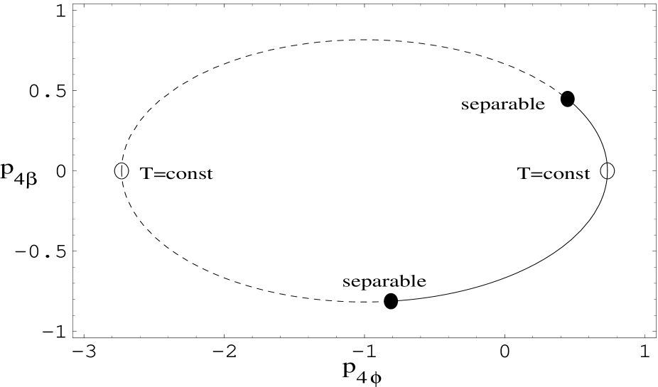
Figure 1: The dilaton and T–modulus expansion coefficients in the four–dimensional string frame for the solutions given in the text. The solid dots correspond to the separable solutions, the circles to the solutions with constant T–modulus. The solid line represents solutions with $p_{4\beta}-p_{4\phi}<0$, the dashed line represents those with $p_{4\beta}-p_{4\phi}>0$.

Let us now discuss the time evolution for the solutions represented in Fig. 1 in the negative–time branch. We start at $t_{4}\rightarrow-\infty$, assuming an effective four–dimensional description at this time. All solutions will, of course, eventually develop large higher–derivative ($\alpha^{\prime}$) corrections as $t_{4}\rightarrow 0$. For example, the product of the “momenta” $\dot{\alpha_{4}}$, $\dot{\beta_{4}}$ and $\dot{\phi_{4}}$ times the orbifold size is proportional to $|t_{4}|^{p_{4\beta}-1}$. This increases as $t_{4}\rightarrow 0$ since $|p_{4\beta}|<1$ always. The precise time when the lowest order $\alpha^{\prime}$ approximation is invalidated depends, of course, on initial conditions.

In section 2 we have discussed another sense in which the fifth dimension may become relevant. Namely, the parameter $\epsilon$ and, hence, the excitation of fields in the fifth dimension may become large. At the same time, this implies large loop corrections. As we have seen, $\epsilon\sim|t_{4}|^{p_{4\beta}-p_{4\phi}}$ and, therefore, its qualitative behavior depends on the sign of $p_{4\beta}-p_{4\phi}$. Consequently, unlike the higher–derivative ($\alpha^{\prime}$) corrections discussed above, $\epsilon$ does not always increase in time. Instead, we should distinguish the three cases (for the negative–time branch)

• $p_{4\beta}-p_{4\phi}>0$ : Then $\epsilon$ decreases in time, indicating decreasing bulk excitations/loop corrections. The Calabi–Yau space expands faster than the orbifold. Solutions with this property are represented by the dashed line in Fig. 1.

• $p_{4\beta}-p_{4\phi}=0$ : Then $\epsilon=$ const, corresponding to constant bulk excitations/loop corrections. The Calabi–Yau space expands at the same rate as the orbifold. As discussed this case corresponds precisely to the two exact separable solutions that can be found. These solutions are indicated by the dots in Fig. 1.

• $p_{4\beta}-p_{4\phi}<0$ : Then $\epsilon$ increases in time indicating increasing bulk excitations/loop corrections. The orbifold expands faster than the Calabi–Yau space. The corresponding solutions are represented by the solid line in Fig. 1.

We see that bulk excitations in the fifth dimension are irrelevant in the first two cases, even as we approach the singularity at $t_{4}\rightarrow 0$. Of course, the system will still run into a large curvature regime close to the singularity. We note that the “standard” solution with a constant T–modulus and inflation in the $D=4$ string frame corresponds to the left circle in Fig. 1. Hence, this solution falls into this category. The right circle, on the other hand, corresponds to a deflating solution in the $D=4$ string frame and it falls into the third category.

In general, in this third case, bulk excitations become relevant close to the singularity. Whether that happens before or after the systems enters the large curvature regime depends on initial condition. Let us assume that we first enter a large $\epsilon$ regime while higher derivative corrections are still small. Then, while $\epsilon$ grows, our approximate five–dimensional solution (3.7) quickly becomes invalid. We know that the exact solutions that govern the further evolution have to be non–separating. Consequently, the time evolution and the excitation of bulk modes will be entangled in a complicated way. As we have discussed, we expect this to be described by a five–dimensional action of the type (2.3) possibly with additional higher order corrections. It would, therefore, be interesting to study exact non–separating cosmological solutions of the action (2.3) in the region of large $\epsilon$. Unfortunately, analytic expressions for those solutions are not available and numerical methods might be required.

However, we may try to extract some information about the behavior at large $\epsilon$ by looking at the four–dimensional metrics that, for a given five–dimensional cosmological solution, are induced on the two boundaries. For example, it would be of interest to know whether or not a solution which is accelerated for small $\epsilon$ can, when $\epsilon$ is large, smoothly become decelerated. The answer, unfortunately, is negative, as we now demonstrate. Following ref. [22], let us write a five–dimensional solution in the general form

$$ds_{5}^{2}=-e^{2\nu}dt_{5}^{2}+e^{2\alpha}d{\bf x}^{2}+e^{2\beta}dy^{2}\;,$$ (4.2)

were $\nu$, $\alpha$ and $\beta$ are functions of $t_{5}$ and $y$. Furthermore, we take the dilaton $\phi$ to be a function of $t_{5}$ and $y$. The equations of motion for such an ansatz, following from the action (2.3), have been presented in ref. [22]. Particularly useful for the present purpose is the $55$ component of the Einstein equation which reads explicitly

$$3e^{-2\nu}(\ddot{\alpha}-\dot{\nu}\dot{\alpha}^{2})-3e^{-2\beta}({\alpha^{\prime}}^{2}+\nu^{\prime}\alpha^{\prime})=-\frac{1}{4}e^{-2\nu}\dot{\phi}^{2}-\frac{1}{4}e^{-2\beta}{\phi^{\prime}}^{2}+\frac{1}{6}v^{2}e^{-2\phi}\;.$$ (4.3)

Here the dot (prime) denotes the derivative with respect to $t_{5}$ ($y$). Furthermore, working in the boundary picture, the functions in the above ansatz have to satisfy the following conditions [22]

$$e^{\phi-\beta}\nu^{\prime}\left.\right|_{y=y_{i}}=e^{\phi-\beta}\alpha^{\prime}\left.\right|_{y=y_{i}}=\frac{\sqrt{2}}{6}v\;,\qquad e^{\phi-\beta}\nu^{\prime}\left.\right|_{y=y_{i}}=\sqrt{2}v\;,$$ (4.4)

at the first (second) boundary at $y_{1}=0$ ($y_{2}=\pi\rho$). These conditions arise as a consequence of the $Z_{2}$ orbifolding and the boundary potentials in the five–dimensional action (2.3), as usual. Restricting eq. (4.3) to either one of the boundaries, and using the conditions (4.4), it is easy to show that

$$\ddot{\alpha}_{i}-\dot{\nu}_{i}\dot{\alpha}_{i}+2\dot{\alpha}_{i}^{2}=-\frac{1}{12}\dot{\phi}_{i}^{2}\;.$$ (4.5)

Here the subscript $i$ denotes the value of the respective field at the boundary $i$, that is, for example $\alpha_{i}(t_{5})=\alpha(t_{5},y_{i})$. We note that the various potential terms occurring in the Einstein equation and the boundary conditions (4.4) cancel in this relation. As a consequence, we have no unusual, linear relationship between the Hubble parameter and the boundary stress energy in eq. (4.4). The possibility of such unconventional relations has been first observed in ref. [22]. As a check, we can now verify that the relation (4.5) is satisfied by our approximate five–dimensional solutions. Putting eq. (3.7) in the form (4.2) and restricting to the boundaries, we can read off the following expressions

$$\alpha_{i}=p_{5\alpha}\ln|t_{5}|\mp\frac{1}{12}\epsilon\;,\qquad\phi_{i}=p_{5\phi}\ln|t_{5}|\mp\frac{1}{2}\epsilon\;,\qquad\nu_{i}=\mp\frac{1}{12}\epsilon$$ (4.6)

where the upper (lower) sign refers to the boundary $i=1$ ($i=2$). Here the expansion coefficient $p_{5\alpha}$, $p_{5\beta}$ and $p_{5\phi}$ satisfy the relations (3.10). Inserting these expressions and using (3.10), we can indeed verify that eq. (4.5) is satisfied to linear order in $\epsilon$, as it should be. We can now go further and use the relations (4.5) to deduce properties of the solutions at arbitrary $\epsilon$. In doing so we have to be careful, of course, since presumably not every set of fields $(\alpha_{i},\nu_{i},\phi_{i})$ satisfying (4.5) can be extended to a full five–dimensional solution. However, conversely, every five–dimensional solution gives rise to induced fields on the boundaries that do satisfy eq. (4.5). It is this latter connection that we are going to use. We introducing the boundary Hubble parameters $H_{i}=\dot{\alpha}_{i}$ and choose the five–dimensional time coordinate $t_{5}$ such that is becomes comoving time upon restriction to the boundaries. This implies $\nu_{i}=0$ and, hence, eq. (4.5) can be written in the form

$$\dot{H}_{i}=-\left(2H_{i}^{2}+\frac{1}{12}\dot{\phi_{i}}^{2}\right)\;.$$ (4.7)

We conclude that $\dot{H}_{i}$ is always negative. Furthermore, the criterion (4.1) for accelerated evolution can be brought into the form $\mbox{sign}(\dot{H}_{i}+H_{i}^{2})=\mbox{sign}(H_{i})$. From eq. (4.7) we conclude that $\dot{H}_{i}+H_{i}^{2}<0$, always. Therefore, the evolution is accelerated exactly if $H_{i}<0$. In this case, the boundaries deflate. On the other hand, for expanding boundaries, $H_{i}>0$, the evolution must be decelerated. Hence, a five–dimensional solution which changes from acceleration to deceleration implies a transition from $H_{i}<0$ to $H_{i}>0$ for the boundary Hubble rates. This, however, cannot happen in a continuous manner since $\dot{H}_{i}<0$. We conclude that a transition from acceleration to deceleration does not take place, even for large values of $\epsilon$. We note, however, that the physically less interesting transition from deceleration to acceleration is not excluded from the above argument. In conclusion, we have shown that the solutions of our five–dimensional theory do not evolve from acceleration to deceleration. This results holds for arbitrarily large $\epsilon$ corrections but only to lowest order in $\alpha^{\prime}$. It is quite conceivable that the inclusion of higher order $\alpha^{\prime}$ corrections can change this situation similarly to what happens in four dimensions [34, 38]. Some of those $\alpha^{\prime}$ correction arise on the boundaries of the five–dimensional theory and, hence, lead to further bulk inhomogeneities. It would be interesting to generalize the present work by including those corrections.

Acknowledgments A. L. is supported by the European Community under contract No. FMRXCT 960090. B. A. O. is supported in part by DOE under contract No. DE-AC02-76-ER-03071 and by a Senior Alexander von Humboldt Award.

References

- [1] M. Mueller, Nucl. Phys. B337 (1990) 37.
- [2] M. Gasperini and G. Veneziano, Astropart. Phys. 1 (1993) 317; R. Brustein and G. Veneziano, Phys. Lett. B329 (1994) 429.
- [3] For a more recent account see : G. Veneziano, “Inflating, Warming Up, and Probing the Pre–Bangian Universe”, CERN-TH-99-22, hep-th/9902097 and references therein.
- [4] For a recent review see : J. E. Lidsey, D. Wands and E. J.Copeland, Superstring Cosmology, PU-RCG-99-9, hep-th/9909061.
- [5] A. Lukas, B. A. Ovrut, K.S. Stelle and D. Waldram, hep-th/9803235, Phys. Rev. D59 (1999) 086001.
- [6] J. Ellis, Z. Lalak, S. Pokorski and W. Pokorski, hep-ph/9805377, Nucl. Phys. B540 (1999) 149.
- [7] A. Lukas, B. A. Ovrut, K. S. Stelle and D. Waldram, hep-th/9806051, Nucl. Phys. B552 (1999) 246.
- [8] P. Hořava and E. Witten, hep-th/9510209, Nucl. Phys. B460 (1996) 506.
- [9] P. Hořava and E. Witten, hep-th/9603142, Nucl. Phys. B475 (1996) 94.
- [10] E. Witten, hep-th/9512219, Nucl. Phys. B463 (1996) 383.
- [11] P. Hořava, hep-th/9608019, Phys. Rev. D54 (1996) 7561.
- [12] A. Lukas, B. A. Ovrut and D. Waldram, hep-th/9608195, Phys. Lett. B393 (1997) 65.
- [13] N. Kaloper, hep-th/9609087, Phys. Rev. D55 (1997) 3394.
- [14] H. Lü, S. Mukherji, C. N. Pope and K. W. Xu, hep-th/9610107, Phys. Rev. D55 (1997) 7926.
- [15] A. Lukas, B. A. Ovrut and D. Waldram, hep-th/9610238, Nucl. Phys. B495 (1997) 365.
- [16] A. Lukas, B.A. Ovrut and Daniel Waldram, hep-th/9806022, Phys. Rev. D60 (1999) 086001.
- [17] H. S. Reall, hep-th/9809195, Phys. Rev. D59 (1999) 103506.
- [18] H. A. Chamblin and H. S. Real, hep-th/9903225 , Nucl. Phys. B562 (1999) 133.
- [19] J. E. Lidsey, gr-qc/9911066, Class. Quant. Grav. 17 (2000) L39.
- [20] M. P. Dabrowski, Kasner Asymptotics of Mixmaster Hořava–Witten Cosmology, hep-th/9911217.
- [21] U. Ellwanger, Cosmological Evolution in Compactified Hořava–Witten Theory by Matter on the Branes, LPT-ORSAY-00-02, hep-th/0001126.
- [22] A. Lukas, B.A. Ovrut and Daniel Waldram, hep-th/9902071, Phys. Rev. D61 (2000) 023506.
- [23] P. Binetruy, C. Deffayet and D. Langlois, Nonconventional Cosmology from a Brane Universe, LPT-ORSAY-99-25, hep-th/9905012.
- [24] T. Nihei, hep-ph/9905487, Phys. Lett. B465 (1999) 81.
- [25] N. Kaloper, hep-th/9905210, Phys. Rev. D60 (1999) 123506.
- [26] P. Kanti, I. I. Kogan, K. A. Olive and M. Pospelov, hep-ph/9909481, Phys. Lett. B468 (1999) 31.
- [27] T. Shiromizu, K. Maeda and M. Sasaki, The Einstein Equation on the 3–Brane World, DAMTP-1999-150, gr-qc/9910076.
- [28] P. Binetruy, C. Deffayet, U. Ellwanger and D. Langlois, Brane Cosmological Evolution in a Bulk with Cosmological Constant, LPT-ORSAY-99-87, hep-th/9910219.
- [29] C. Csaki, M. Graesser, L. Randall and J. Terning, Cosmology of Brane Models with Radion Stabilization, SCIPP-99-49, hep-ph/9911406.
- [30] P. Kanti, I. I. Kogan, K. A. Olive and M. Pospelov, Single Brane Cosmological Solutions with a Stable Compact Extra Dimension, UMN-TH-1829-99, hep-ph/9912266.
- [31] T. Banks, W. Fischler and L. Motl, hep-th/9811194, J. High Energy Phys. 01 (1999) 019.
- [32] M. B. Green, M. Gutperle, Nucl. Phys. B498 (1997) 195; M. B. Green, M. Gutperle and P. Vanhove, Phys. Lett. B409 (1997) 177.
- [33] A. Lukas, B.A. Ovrut and Daniel Waldram, hep-th/9710208, Nucl. Phys. B532 (1998) 43.
- [34] I. Antoniadis, J. Rizos and K. Tamvakis, hep-th/9305025, Nucl. Phys. B415 (1994) 497.
- [35] J. Ellis, N. Kaloper, K. A. Olive and J. Yokoyama, hep-ph/9807482, Phys. Rev. D59 (1999) 103503.
- [36] A. Lukas and B.A. Ovrut, Symmetric Vacua in Heterotic M–Theory, OUTP-99-37-P, hep-th/9908100.
- [37] M. Gasperini and G. Veneziano, hep-th/9309023, Mod. Phys. Lett A8 (1993) 3701.
- [38] C. Cartier, E.J. Copeland and R. Madden, hep-th/9910169 J. High Energy Phys. 01 (2000) 035.