On the Supersymmetry and Gauge Structure of Matrix Theory

Y. Kazama and T. Muramatsu

Institute of Physics, University of Tokyo,
Komaba, Meguro-ku, Tokyo 153-8902 Japan

Abstract

Supersymmetric Ward identity for the low energy effective action in the standard background gauge is derived for arbitrary trajectories of supergravitons in Matrix Theory. In our formalism, the quantum-corrected supersymmetry transformation laws of the supergravitons are directly identified in closed form, which exhibit an intricate interplay between supersymmetry and gauge (BRST) symmetry. As an application, we explicitly compute the transformation laws for the source-probe configuration at 1-loop and confirm that supersymmetry fixes the form of the action completely, including the normalization, to the lowest order in the derivative expansion.

1 Introduction

By now a considerable amount of evidence has been accumulated for the Matrix theory for M-theory, originally proposed by Banks, Fischler, Shenker and Susskind[1] and later re-interpreted by Susskind[2] in the framework of discrete light-cone quantization. In particular, just to mention only the direct comparison with eleven dimensional supergravity, complete agreement for the multi-graviton scattering (including the recoil effects) at 2-loop[3, 4] and that for the two-body potential between arbitrary fermionic as well as bosonic objects at 1-loop [5] can be cited as highly non-trivial and remarkable.

Despite such impressive pieces of evidence as well as general supportive arguments [6, 7], the deep reason and the mechanism of the agreement are yet to be fully understood. Evidently, one of the keys should be the understanding of the structure and the role of the symmetries. The well-known symmetries present both in the Matrix theory and in the supergravity theory are the global $Spin(9)$ invariance, the CPT invariance and the invariance under 16 supersymmetries. Perhaps less familiar is the generalized conformal invariance[8, 9, 10], the generalization of the conformal symmetry that plays the major role in the AdS/CFT correspondence of Maldacena[11]. Besides these symmetries, the supergravity possesses the general coordinate invariance while the Matrix theory has the Yang-Mills type gauge symmetry, which must be deeply connected. Finally, although not yet clearly identified, the agreement of the multi-body scattering amplitudes strongly suggests that the eleven dimensional Lorentz invariance is present in a highly non-trivial manner in the Matrix theory.

Except for the eleven dimensional Lorentz invariance, the above-mentioned symmetries of the Matrix theory are easily recognized in the original action. However, since the supergravity interactions between various objects arise only after introducing the corresponding backgrounds and integrating out the quantum fluctuations around them, the realizations of these symmetries are in general modified for the effective action of interest. Besides, being an off-shell quantity, the form of the effective action depends on the choice of the gauge as well as on the definition of the fields. Further, there is always a vast degree of ambiguities as one can add total derivatives. For these reasons, the study of how the symmetries govern the structure of the effective action becomes quite non-trivial.

In this article, we shall focus on the supersymmetry (SUSY), considered to be the most powerful among the ones listed above. In fact it has been claimed that a large degree of SUSY, ${\cal N}=16$, present in the theory imposes strong restrictions on the form of the effective action and leads to a number of “non-renormalization theorems”[12]–[17]. However, upon close examinations one finds that such assertions in the existing literature can still be challenged. This is essentially due to the lack of completely off-shell consideration. As we shall elaborate in some detail in Sec. 3, to understand precisely to what extent SUSY is responsible in determining the effective action, one must allow the background fields to have arbitrary time-dependence. This in turn inevitably leads to the necessity of examining the gauge (BRST) symmetry, another important ingredient of Matrix theory, as SUSY and gauge symmetry are known to be intimately intertwined off-shell. Such an analysis has not been performed in the past.

What makes the off-shell analysis difficult is that we do not as yet have the off-shell unconstrained superfield formulation in the case of ${\cal N}=16$ supersymmetry. This prompts us to resort to the conventional means, namely the Ward identity for the symmetries in question. In order to be able to check against the available explicit result for the effective action, one would like to obtain the Ward identity in so-called the “background gauge”, in which all the calculations have been performed. Although the derivation of such a Ward identity is expected to be a text-book matter, this was not to be: One must carefully disentangle the dependence on the background field of the effective action by making use of BRST Ward identities. The result is a somewhat complicated Ward identity, in which the supersymmetry and the BRST symmetry are intertwined. A notable feature of our Ward identity is that one can read off the effective quantum-corrected SUSY transformations in closed form and this should serve as a starting point of various truly off-shell investigations. As a simple application, we compute the transformation laws to the lowest order in the derivative expansion at 1-loop and analyze the restriction imposed by SUSY on the effective action for a background with arbitrary time-dependence, to the corresponding order. We find that at this order the effective action is indeed fully determined by the requirement of supersymmetry, which agrees with the explicit calculation[18] including the normalization.

The rest of the paper is organized as follows: In Sec. 2, we recall the symmetries of the original action of Matrix theory and the BRST symmetry associated with the background gauge fixing. Then in Sec. 3 we make some important remarks on the determination of the effective action and its symmetries, to emphasize the necessity of completely off-shell analysis. Having clarified the issue, we proceed in Sec. 4 to the derivation of the SUSY Ward identity for the effective action in the background gauge. By carefully separating the different origins of the dependence on the background field, we obtain the desired Ward identity together with the closed expressions for the effective SUSY transformation laws. This constitutes the main result of this work. As an application, we explicitly work out in Sec. 5 the SUSY transformation laws to the lowest order in the derivative expansion at 1-loop and show that the effective action to the corresponding order is completely determined by the Ward identity. Sec. 6 is devoted to a short summary and discussions of future problems.

2 Action and its Symmetries

Let us begin by recalling the action of the Matrix theory and its symmetries, which at the same time serves to set our notations.

The basic action of the Matrix theory can be written as

$$S_{0} = \mbox{Tr}\int\!dt\Biggl{\{}{1\over 2}\left[D_{t},X_{m}\right]^{2}+{g^{2}\over 4}\left[X_{m},X_{n}\right]^{2}$$ (2.1)

$$\qquad+{i\over 2}\Theta^{T}\left[D_{t},\Theta\right]+{g\over 2}\Theta^{T}\gamma^{m}\left[X_{m},\Theta\right]\Biggr{\}}\,,$$

$$D_{t} = \partial_{t}-igA\,,$$ (2.2)

where $N\times N$ hermitian matrices $X_{ij}^{m}(t)\,,A_{ij}(t)\,,\Theta_{\alpha,ij}(t)$ stand for the bosonic, the gauge, and the fermionic fields respectively. The middle Latin indices $m,n,\ldots$, running from $1$ to $9$, denote the spatial directions, while the Greek letters such as $\alpha\,,\beta=1\sim 16$ are used for the $SO(9)$ spinor indices. The $16\times 16$ $\gamma$-matrices $\gamma^{m}$ are real symmetric and satisfy $\left\{\gamma^{m},\gamma^{n}\right\}=\delta^{mn}$.

To facilitate the quantum computations, it is convenient to define the theory by going to the “Euclidean formulation”. Introduce the Euclidean time $\tau$, the gauge field $\widetilde{A}$, and the action $\widetilde{S}_{0}$ by

$$\tau \equiv it\,,\qquad\widetilde{A}\equiv-iA\,,\qquad\widetilde{S}_{0}\equiv-iS_{0}\,.$$ (2.3)

Then the action and the covariant derivative become

$$\widetilde{S}_{0} = \mbox{Tr}\int\!d\tau\Biggl{\{}{1\over 2}\left[D_{\tau},X_{m}\right]^{2}-{g^{2}\over 4}\left[X_{m},X_{n}\right]^{2}$$ (2.4)

$$\qquad+{1\over 2}\Theta^{T}\left[D_{\tau},\Theta\right]-{1\over 2}g\Theta^{T}\gamma^{m}\left[X_{m},\Theta\right]\Biggr{\}}\,,$$

$$D_{\tau} = \partial_{\tau}-ig\widetilde{A}\,.$$ (2.5)

Besides the obvious $Spin(9)$ symmetry, this action is invariant under the following transformations:

1. Gauge transformations with a gauge parameter matrix $\Lambda$:

   $$\delta_{\Lambda}\widetilde{A} = \left[D_{\tau},\Lambda\right]\,,\qquad\delta_{\Lambda}X_{m}=ig\left[\Lambda,X_{m}\right]\,,\qquad\delta_{\Lambda}\Theta=ig\left[\Lambda,\Theta\right]\,.$$ (2.6)

2. Supersymmetry transformations with a spinor parameter $\epsilon_{\alpha}$:

   $$\delta_{\epsilon}\widetilde{A} = \epsilon^{T}\Theta\,,\qquad\delta_{\epsilon}X^{m}=-i\epsilon^{T}\gamma^{m}\Theta\,,$$ (2.7)

   $$\delta_{\epsilon}\Theta = i\left(\left[D_{\tau},X_{m}\right]\gamma^{m}+{g\over 2}\left[X_{m},X_{n}\right]\gamma^{mn}\right)\epsilon$$ (2.8)

   where $\gamma^{mn}\equiv{1\over 2}\left[\gamma^{m},\gamma^{n}\right]$ is real anti-symmetric. When the system possesses symmetries other than the supersymmetry, the supersymmetry algebra may close not only on the space-time translation but also on the generators of such additional symmetries. In fact in the present case it is well-known that it involves the gauge symmetry with a field-dependent gauge function. For example on $\widetilde{A}$,

   $$\left[\delta_{\epsilon},\delta_{\lambda}\right]\widetilde{A} = -2i\epsilon^{T}\lambda\,\partial_{\tau}\widetilde{A}+\delta_{\Lambda}\widetilde{A}\,,$$ (2.9)

   $$\mbox{where}\qquad\Lambda = -2i(\epsilon^{T}\gamma^{m}\lambda X_{m}-\epsilon^{T}\lambda\widetilde{A})\,,$$ (2.10)

   and similarly for the other fields. Moreover, for a system with ${\cal N}=16$ supersymmetry, such as the Matrix theory, formulation in terms of unconstrained superfields is not known and hence the algebra closes only up to the equations of motion in general. Thus it is expected that the proper understanding of the supersymmetry of the Matrix theory must include the analysis of these non-trivial features.

3. Generalized conformal transformations: If we rescale the fields $X_{m}$ and $\widetilde{A}$ by a factor of $g$, such as $X_{m}\rightarrow X_{m}/g$, and allow $g$ to depend on $\tau$ to a linear order, $\widetilde{S}_{0}$ is invariant under a generalization of the conformal transformations[8] [10]. In particular, the invariance under the special conformal transformation defined by

   $$\delta_{K}\widetilde{A} = 2\epsilon\tau\widetilde{A}\,,\qquad\delta_{K}X_{m}=2\epsilon\tau X_{m}\,,\qquad\delta_{K}\Theta_{\alpha}=0$$

   $$\delta_{K}\tau = -\epsilon\tau^{2}\,,\qquad\delta_{K}g=3\epsilon\tau g\,,$$ (2.11)

   $$\epsilon = \mbox{an infinitesimal bosonic parameter}\,,$$

   imposes a useful restriction on the form of the effective action.

Besides these well-established symmetries, the remarkable agreement between the 11-dimensional supergravity calculations and the 2-loop Matrix theory calculations for multi-body scattering processes[3] strongly suggests that the Matrix theory actually possesses 11-dimensional Lorentz symmetry in a highly non-trivial manner.

In this article, we shall focus on how the first two of these symmetries, which are intimately intertwined, are implemented in the quantum effective action of the supergravitons. In the M-theory interpretation of the Matrix theory, the coordinates and the spin degrees of freedom of these supergravitons are represented by the diagonal backgrounds for $X^{m}$ and $\Theta_{\alpha}$ respectively. We shall denote them by $B_{m}$ and $\theta_{\alpha}$ respectively and separate them from the quantum parts $Y_{m}$ and $\Psi_{\alpha}$ as

$$X_{m} = {1\over g}B_{m}+Y_{m}\,,$$ (2.12)

$$\Theta_{\alpha} = {1\over g}\theta_{\alpha}+\Psi_{\alpha}\,.$$ (2.13)

As was already emphasized in the introduction and will be further elaborated in the next section, it is important to take $B_{m}(\tau)$ and $\theta_{\alpha}(\tau)$ as arbitrary backgrounds, not satisfying any equations of motion. Only in this way we can unambiguously determine how much restrictions are imposed by the supersymmetry on the effective action for these background fields.

To quantize the theory, we need to fix the gauge. Although our derivation of the Ward identity, to be presented in Sec. 4, can be readily adapted to any choice of gauge, the actual computations are extremely cumbersome except in the standard background gauge. It is specified by the gauge-fixing function of the form

$$G = -\partial_{\tau}\widetilde{A}+i\left[B^{m},X_{m}\right]\,.$$ (2.14)

In fact essentially all the existing explicit calculations have been performed in this gauge. However, as it will become clear, the naive use of this gauge leads to a subtle but important complication in deriving the correct Ward identity. To avoid this problem, we will tentatively use a different function $\widetilde{B}_{m}$ in place of $B_{m}$ and write the gauge-fixing function as

$$\widetilde{G} = -\partial_{\tau}\widetilde{A}+i\left[\widetilde{B}^{m},X_{m}\right]\,.$$ (2.15)

Later at an appropriate stage, we will set $\widetilde{B}_{m}=B_{m}$.

The corresponding ghost action can be readily obtained by the standard BRST method. The BRST transformations for the quantum part of the fields are given by

$$\delta_{B}\widetilde{A} = \left[D_{\tau},C\right]\,,\qquad\delta_{B}Y_{m}=-ig\left[X_{m},C\right]\,,$$

$$\delta_{B}\Psi = ig\left\{C,\Theta\right\}\,,$$ (2.16)

$$\delta_{B}C = igC^{2}\,,\qquad\delta_{B}\overline{C}=ib\,,\qquad\delta_{B}b=0\,.$$

$C$, $\overline{C}$ and $b$ are, respectively, the ghost, the anti-ghost and the Nakanishi-Lautrup auxiliary fields. The background fields are not transformed. Then the combined gauge-ghost action $\widetilde{S}_{gg}$ is generated by

$$\widetilde{S}_{gg} = \delta_{B}\mbox{Tr}\int\!d\tau\left[{1\over i}\overline{C}\left(\widetilde{G}-{\alpha\over 2}b\right)\right]\,.$$ (2.17)

We will henceforth set the gauge parameter $\alpha$ to be 1. This leads, after integrating over the $b$ field, to the familiar gauge-ghost action

$$\widetilde{S}_{gg} = \mbox{Tr}\int\!d\tau{1\over 2}\left(-\partial_{\tau}\widetilde{A}+i\left[\widetilde{B}^{m},X_{m}\right]\right)^{2}$$ (2.18)

$$\qquad-i\mbox{Tr}\int\!d\tau\left(\overline{C}\partial_{\tau}\left[D_{\tau},C\right]-g\overline{C}\left[\widetilde{B}^{m},\left[X_{m},C\right]\right]\right)\,.$$

3 Remarks on the Determination of Effective Action and its Symmetries

Before starting the derivation of the off-shell supersymmetry Ward identity, we wish to make some important remarks on the determination of the effective action and its symmetries, which point to the necessity of off-shell analysis. Although many of the remarks will apply for general backgrounds, for clarity of discussions we shall consider the so-called “source-probe configuration”. In the case of $U(N+1)$ gauge group, it is defined as the situation where a probe supergraviton interacts with $N$ supergravitons situated at the origin that act as a heavy source. The background fields representing this situation are

$$B_{m} = {\rm diag}\,(r_{m},0,0,\ldots,0)\,,\qquad\theta_{\alpha}={\rm diag}\,(\theta_{\alpha},0,0,\ldots,0)\,.$$ (3.19)

Here, $r_{m}$ represents the coordinate of the probe and $\theta_{\alpha}$ its spin content. As usual, the spin of the source is neglected.

As already emphasized in the introduction, the primary feature of Matrix theory is that it generates the supergravity interactions among various objects only after (i) introducing the corresponding backgrounds and (ii) integrating over the quantum fluctuations around them. Because of this, realizations of the symmetries of the effective theory are in general modified non-trivially. Besides, being an off-shell quantity, the form of the effective action is affected by (A) the gauge choice, (B) the (re)definition of the fields, and (C) the freedom of adding total derivatives. Of course the on-shell S-matrix elements do not depend on these factors. However, the determination of the full ( i.e. quantum-corrected) on-shell condition itself requires the knowledge of the off-shell effective action. Thus, in order to understand the symmetry structure of the effective theory fully, it is necessary to perform an off-shell analysis with (A) $\sim$ (C) properly taken into account.

Now since an exact analysis is practically impossible, one often needs to make some approximations. In doing so, one must make sure that they are logically consistent for one’s aim. For the present purpose, some of the often used approximations are not appropriate. For example, the eikonal approximation, where one tries to reconstruct the effective action from the eikonal phase shift, can be dangerous and misleading. In fact the answer depends on the form of the effective Lagrangian assumed. As a simple illustration, consider the 1-loop eikonal phase shift [19] for $v\ll 1$ given by

$$\widetilde{\Gamma}_{1}^{e} = -{v^{3}\over b^{6}}+0\times{v^{5}\over b^{10}}-{3\over 2}{v^{7}\over b^{14}}+{\cal O}(v^{9})$$

$$r_{m} = v_{m}\tau+b_{m}\,,\quad v\cdot b=0\,,\qquad b_{m}=\mbox{impact parameter}\,.$$

If one assumes the effective Lagrangian to be of the form ${\cal L}={\cal L}(v,r)$, then the effective action that reproduces this phase shift is uniquely determined to be

$$\widetilde{S}_{1} = \int\!d\tau\left(-{15\over 16}{v^{4}\over r^{7}}+0\times{v^{6}\over r^{11}}-{9009\over 4096}{v^{8}\over r^{15}}+{\cal O}(v^{10})\right)\,.$$

However, even restricting to ${\cal O}(v^{4})$, the most general form allowed for the effective action contains 6 independent structures, after eliminating total-derivative ambiguities:

$$\widetilde{S}_{1} = \int\!d\tau\left(A{v^{4}\over r^{7}}+B{v^{2}(v\cdot r)^{2}\over r^{9}}+C{(v\cdot r)^{4}\over r^{11}}\right.$$

$$\left.+D{v^{2}(a\cdot r)\over r^{7}}+E{(a\cdot r)^{2}\over r^{7}}+F{a^{2}\over r^{5}}\right)\,.$$

On the other hand, there is only one condition, $-(15/16)=A+(1/7)B+(1/21)C$, required for the correct phase shift, and hence 5 parameters remain undetermined. The situation at ${\cal O}(v^{6})$ is even more striking. Although the eikonal phase shift vanishes, the explicit computation reveals that there are 5 non-vanishing independent structures present in the effective action[20].

It should be clear from these illustrations that the only logically consistent procedure, not affected by the total-derivative ambiguities, is to use off-shell backgrounds with arbitrary $\tau$-dependence and to classify terms by derivative expansion according to the “order” defined by

order $$= \mbox{\# of $\partial_{\tau}$}+{1\over 2}\mbox{\# of fermions}\,.$$ (3.20)

If necessary, one may combine this with the usual loop expansion.

Having emphasized the importance of off-shell considerations, we now make some related comments on the general arguments on the restrictions imposed by supersymmetry, often referred to as SUSY non-renormalization theorems. They can be roughly classified into two categories.

The first type of argument, devised by Paban et al [12], relies on the closure property of SUSY transformations. For example, at ${\cal O}(v^{2})$ they first make a choice of the definition of the fields so that the action takes the form $\displaystyle\int\!d\tau f(r)v^{2}$ and take the ${\cal O}(v^{0})$ SUSY transformation laws in that basis to be the standard ones without any correction, $\delta_{\epsilon}r^{m}=-i\epsilon\gamma^{m}\theta\,,\delta_{\epsilon}\theta_{\alpha}=i(v\!\!\!/\epsilon)_{\alpha}$. Then demanding that the closure is canonical, namely $\left[\delta_{\epsilon},\delta_{\lambda}\right]=2\lambda^{T}\epsilon\partial_{\tau}$, they show that there cannot be a correction to the transformation laws at ${\cal O}(v^{2})$ and hence the ${\cal O}(v^{2})$ effective action is tree-exact. Although the argument is quite simple and plausible, it is unclear why the closure should be canonical off-shell and further it is not obvious if the ${\cal O}(v^{0})$ transformation laws must be of the standard form in a particular basis adopted. In general, field redefinitions affect the form of the SUSY transformations and hence they must be considered as a pair.

The other type of argument is known as the SUSY completion method, which makes use of the chain of relations produced among terms with different number of $\theta$’s by SUSY transformations. For example, at ${\cal O}(v^{4})$ one expects relations of the form

$$v^{4}\longleftarrow v^{3}\theta^{2}\longleftarrow v^{2}\theta^{4}\longleftarrow v\theta^{6}\longleftarrow\theta^{8}\,.$$ (3.21)

By showing that the top form, $\theta^{8}$ term in this case, is not renormalized beyond 1-loop, one wishes to infer the non-renormalization of all the other terms in the chain, in particular the $v^{4}$ term. This method appears efficient, but some care is needed in drawing firm conclusions. One problem is that sometimes the chain starting from the top form stops at an intermediate stage. Put differently, one may form a super-invariant not containing the top form. An example already occurs at ${\cal O}(v^{2})$, where the tree-level expression $\displaystyle\int\!d\tau\left((v^{2}/2g^{2})+(\theta\dot{\theta}/2g^{2})\right)$ is SUSY-complete without a $\theta^{4}$ term. More non-trivial example is seen at ${\cal O}(v^{6})$: Although $\theta^{12}$ term was shown to vanish[13] at 1-loop, the bosonic contribution at ${\cal O}(v^{6})$ nonetheless exists[20].

An attempt at filling this gap was made in [16]. In this work all the connections in the chain (3.21) were examined and it was concluded that SUSY is indeed powerful enough to fix the effective action at this order up to an overall constant. Again one must be cautious in accepting this conclusion: In this analysis $v$ and $\theta$ were taken to be $\tau$-independent and hence the assumed form of the effective Lagrangian was not the most general one allowed in the proper derivative expansion with arbitrary backgrounds. Later it was recognized[18], however, that the higher derivative terms neglected in this analysis can actually be absorbed into the tree-level Lagrangian by a suitable field re-definition, which appeared to resurrect the validity of the analysis made in [16]. Unfortunately, the problem still persists: By such a field re-definition the higher derivatives are simply shifted into the SUSY transformation laws and one must reanalyze the issue with such modifications.

Thus one sees that although the existing analyses are highly plausible they are not air-tight. In view of the importance of precise understanding of the role of supersymmetry and its connection with gauge symmetry, it is desirable to perform an unambiguous off-shell analysis with arbitrary backgrounds. This motivates us to the study of the Ward identity, to be described in the next two sections.

4 SUSY Ward Identity for the Effective Action in the Background Gauge

Having argued the importance of off-shell analysis for arbitrary trajectories, we shall now derive the SUSY Ward identity for the effective action $\widetilde{\Gamma}$ in the standard background gauge, (2.14), used exclusively in the actual computations.

To make use of the well-established method, let us further split the quantum fluctuations $Y_{m}$ and $\Psi_{\alpha}$ into two parts, the diagonal and the off-diagonal, in the manner

$$Y_{m,ij}={\widehat{y}_{m,i}\over g}\delta_{ij}+\widehat{Y}_{m,ij}\,,\qquad\Psi_{\alpha,ij}={\widehat{\psi}_{\alpha,i}\over g}\delta_{ij}+\hat{\Psi}_{\alpha,ij}\,,$$ (4.22)

and introduce the sources only for the diagonal fields:

$$\widetilde{S}_{s}=\int\!d\tau\left(J_{m,i}\widehat{y}_{m,i}+\eta_{\alpha,i}\widehat{\psi}_{\alpha,i}\right)\,.$$ (4.23)

The Euclidean generating functionals are defined by

$$\widetilde{Z}[J,\eta] = \int\!{\cal D}\mu\,\exp\left(-\widetilde{S}_{tot}\right)=\exp\left(-\widetilde{W}[J,\eta]\right)\,,$$ (4.24)

$$\widetilde{S}_{tot} \equiv \widetilde{S}_{0}+\widetilde{S}_{gg}+\widetilde{S}_{s}\,,\qquad{\cal D}\mu\equiv{\cal D}\!\widetilde{A}\,{\cal D}Y\,{\cal D}\Psi\,{\cal D}C\,{\cal D}\overline{C}\,,$$

where $\widetilde{W}[J,\eta]$ is the one for the connected functions. By making the change of integration variables corresponding to the supersymmetry transformations, one obtains the primitive form of the Ward identity

$$0=\langle\delta_{\epsilon}\widetilde{S}_{gg}\rangle+\langle\delta_{\epsilon}\widetilde{S}_{s}\rangle\,.$$ (4.25)

Here and in what follows, $\langle{\cal O}\rangle$ for an operator ${\cal O}$ means

$$\langle{\cal O}\rangle={\displaystyle\int\!{\cal D}\mu\,{\cal O}e^{-\widetilde{S}_{tot}}\over\displaystyle\int\!{\cal D}\mu\,e^{-\widetilde{S}_{tot}}}\,.$$ (4.26)

We now rewrite this identity (4.25) in terms of the generating functional $\widetilde{\Gamma}$, which is 1PI (1-particle-irreducible) with respect to the diagonal fields. Define as usual the classical fields and $\widetilde{\Gamma}$ by

$$y_{m,i(\tau)} \equiv {\delta\widetilde{W}\over\delta J_{m,i}(\tau)}\,,\qquad\psi_{\alpha,i}(\tau)\equiv{\delta\widetilde{W}\over\delta\eta_{\alpha,i}(\tau)}\,,$$ (4.27)

$$\widetilde{\Gamma}[y,\psi] \equiv W[J,\eta]-\int\!d\tau(J_{m,i}y_{m,i}+\eta_{\alpha,i}\psi_{\alpha,i})\,.$$ (4.28)

Then the sources are expressed in terms of $\widetilde{\Gamma}$ as

$$J_{m,i}(\tau)=-{\delta\widetilde{\Gamma}\over\delta y_{m,i}(\tau)}\,,\qquad\eta_{\alpha,i}(\tau)={\delta\widetilde{\Gamma}\over\delta\psi_{\alpha,i}(\tau)}\,.$$ (4.29)

Therefore, the contribution to the Ward identity from the variation of the source action can be written as

$$\langle\delta_{\epsilon}\widetilde{S}_{s}\rangle=\int\!d\tau\left(-{\delta\widetilde{\Gamma}\over\delta y_{m,i}(\tau)}\langle\delta_{\epsilon}\widehat{y}_{m,i}(\tau)\rangle+{\delta\widetilde{\Gamma}\over\delta\psi_{\alpha,i}(\tau)}\langle\delta_{\epsilon}\widehat{\psi}_{\alpha,i}(\tau)\rangle\right)\,.$$ (4.30)

As for the contribution $\langle\delta_{\epsilon}\widetilde{S}_{gg}\rangle$ from the gauge-ghost part, a direct calculation yields a rather complicated expression, which constitutes an inhomogeneous term in the Ward identity regarded as a functional integro-differential equation for $\widetilde{\Gamma}$. This is undesirable since what we wish to understand is how the supersymmetry acts on the effective action $\widetilde{\Gamma}$. Fortunately, it was noted long ago [22] in the context of four-dimensional super Yang-Mills theory that one can reexpress such a term in a form similar to (4.30). The first step is to note that the supersymmetry transformations (2.7) and (2.8) commute with the BRST transformation (2.16) on all the fields, as can be checked straightforwardly. Therefore, starting from (2.17), $\langle\delta_{\epsilon}\widetilde{S}_{gg}\rangle$ can be written as

$$\langle\delta_{\epsilon}\widetilde{S}_{gg}\rangle = \langle\delta_{\epsilon}\delta_{B}\mbox{Tr}\int\!d\tau\left[{1\over i}\overline{C}\left(\widetilde{G}-{1\over 2}b\right)\right]\rangle$$ (4.31)

$$= \langle\delta_{B}\delta_{\epsilon}\mbox{Tr}\int\!d\tau\left[{1\over i}\overline{C}\left(\widetilde{G}-{1\over 2}b\right)\right]\rangle=\langle\delta_{B}{\cal O}_{\epsilon}\rangle\,,$$

where

$${\cal O}_{\epsilon}\equiv{1\over i}\mbox{Tr}\int\!d\tau\overline{C}\delta_{\epsilon}\widetilde{G}$$ (4.32)

is a fermionic composite operator. This expression, being an expectation value of a BRST-exact form, vanishes in the ordinary vacuum. However, in the presence of external sources, it becomes proportional to the sources, and hence to the functional derivatives of $\widetilde{\Gamma}$. Let us collectively denote by $\phi$ and $J$ the basic fields and the corresponding sources respectively and consider the generating functional with a source $j$ for the operator ${\cal O}_{\epsilon}$:

$$Z[J,j]=\int\!{\cal D}\phi\,e^{-(S_{tot}+J\phi+j{\cal O}_{\epsilon})}\,.$$ (4.33)

Now make a change of variables corresponding to the BRST transformation. We get

$$0=\int\!{\cal D}\phi\,((-1)^{|\phi|}J\delta_{B}\phi-j\delta_{B}{\cal O}_{\epsilon})e^{-(S_{tot}+J\phi+j{\cal O}_{\epsilon})}\,,$$ (4.34)

where $|\phi|$ is 0 (1) if $\phi$ is bosonic (fermionic). By differentiating with respect to $j$ once, setting $j=0$, and then expressing the source $J$ in terms of $\widetilde{\Gamma}$, one easily obtains the following BRST Ward identity:

$$\langle\delta_{B}{\cal O}_{\epsilon}\rangle = -\int\!d\tau{\delta\widetilde{\Gamma}\over\delta\phi(\tau)}\langle\delta_{B}\phi(\tau){\cal O}_{\epsilon}\rangle\,.$$ (4.35)

In this way, we get

$$\langle\delta_{\epsilon}\widetilde{S}_{gg}\rangle=-\int\!d\tau\left({\delta\widetilde{\Gamma}\over\delta y_{m,i}(\tau)}\langle\delta_{B}\widehat{y}_{m,i}(\tau){\cal O}_{\epsilon}\rangle+{\delta\widetilde{\Gamma}\over\delta\psi_{\alpha,i}(\tau)}\langle\delta_{B}\widehat{\psi}_{\alpha,i}(\tau){\cal O}_{\epsilon}\rangle\right)\,.$$ (4.36)

Putting all together, we arrive at the following SUSY Ward identity expressed solely in terms of the derivatives of $\widetilde{\Gamma}$:

$$0 = \int\!d\tau\Biggl{(}{\delta\widetilde{\Gamma}\over\delta y_{m,i}(\tau)}(\langle\delta_{\epsilon}\widehat{y}_{m,i}(\tau)\rangle+\langle\delta_{B}\widehat{y}_{m,i}(\tau){\cal O}_{\epsilon}\rangle)$$ (4.37)

$$\qquad-{\delta\widetilde{\Gamma}\over\delta\psi_{\alpha,i}(\tau)}(\langle\delta_{\epsilon}\widehat{\psi}_{\alpha,i}(\tau)\rangle-\langle\delta_{B}\widehat{\psi}_{\alpha,i}(\tau){\cal O}_{\epsilon}\rangle)\Biggr{)}\,.$$

Normally it is now a simple matter to convert this into the desired Ward identity for the effective action as a functional of the backgrounds $B^{m}$ and $\theta_{\alpha}$: One would rewrite the derivatives with respect to $y_{m}$ and $\psi_{\alpha}$ into those with respect to $B^{m}$ and $\theta_{\alpha}$ and then set $y_{m}=\psi_{\alpha}=0$. This procedure is indeed valid for the fermions since $\widehat{\psi}_{\alpha}$ and $\theta_{\alpha}$ always appear in the combination $\widehat{\psi}_{\alpha}+\theta_{\alpha}$ in the original action and it is a simple matter to prove that this gets converted to $\psi_{\alpha}+\theta_{\alpha}$ in $\widetilde{\Gamma}$.

This is not so for the bosonic field. While most of the $B^{m}$ dependence comes from the splitting $X_{m}=(1/g)(B_{m}+\widehat{y}_{m})+\widehat{Y}_{m}$, where $B_{m}$ and $\widehat{y}_{m}$ appear together, $B^{m}$ in the gauge-ghost sector (in the standard background gauge) is not accompanied with $\widehat{y}_{m}$. From the point of view of the Ward identity above, it is an independent extra parameter field which should be distinguished from the bona fide background field. This is why we chose to start out with a different symbol $\widetilde{B}^{m}$ for this field.

Now the problem we face is the following. In order to be able to apply the Ward identity to the case of the standard background gauge, we need to express the dependence on $\widetilde{B}^{m}$ again in the form of the functional derivative of $\widetilde{\Gamma}$ with respect to $B^{m}$. In other words, we must disentangle the two different types of $B^{m}$ dependence buried in the standard background gauge formulation and construct the Ward identity which takes both types of dependence into account. Although this is a technical rather than a conceptual problem, it is again a manifestation of the gauge theory nature of the Matrix theory, which has often been neglected.

The problem can be solved as follows. Since $\widetilde{B}^{m}$ appears only in the gauge-ghost action and the variation with respect to it commutes with the BRST transformation, we get from (2.17)

$${\delta\widetilde{S}_{gg}\over\delta\widetilde{B}^{m,i}(\tau)}=\delta_{B}{\cal O}_{m,i}(\tau)\,,$$ (4.38)

where

$${\cal O}_{m,i}=\sum_{j}\left(\overline{C}_{ji}Y_{m,ij}-\overline{C}_{ij}Y_{m,ji}\right)\,,$$ (4.39)

and $\widetilde{B}^{m,i}$ stands for the diagonal elements $\widetilde{B}^{m}_{ii}$. The expectation value of the left-hand side can be expressed in terms of the generating functional $\widetilde{W}$ as $\delta\widetilde{W}/\delta\widetilde{B}_{m,i}$, which is equal to $\delta\widetilde{\Gamma}/\delta\widetilde{B}_{m,i}$ since it is a parameter field. On the other hand the expectation value of the right-hand side can be treated in exactly the same way as we treated $\delta_{B}{\cal O}_{\epsilon}$. In this way we get the identity

$${\delta\widetilde{\Gamma}\over\delta\widetilde{B}_{m,i}(\tau)} = -\int\!d\tau^{\prime}\Biggl{(}{\delta\widetilde{\Gamma}\over\delta y_{n,j}(\tau^{\prime})}\langle\delta_{B}\widehat{y}_{n,j}(\tau^{\prime}){\cal O}_{m,i}(\tau)\rangle$$ (4.40)

$$\qquad+{\delta\widetilde{\Gamma}\over\delta\psi_{\alpha,j}(\tau^{\prime})}\langle\delta_{B}\widehat{\psi}_{\alpha,j}(\tau^{\prime}){\cal O}_{m,i}(\tau)\rangle\Biggr{)}\,.$$

Now let us replace $y_{m}$ and $\psi_{\alpha}$ with $B_{m}$ and $\theta_{\alpha}$ respectively and then set $y_{m}=\psi_{\alpha}=0$ in the previous Ward identity (4.37) and in the relation (4.40) above. In the limit $\widetilde{B}_{m}\rightarrow B_{m}$, the total variation of $\widetilde{\Gamma}$ with respect to $B_{m}$, which we denote by $\Delta\widetilde{\Gamma}/\Delta B_{m}$ to avoid confusion, is

$${\Delta\widetilde{\Gamma}\over\Delta B_{m,i}(\tau)}=\left({\delta\widetilde{\Gamma}\over\delta B_{m,i}(\tau)}+{\delta\widetilde{\Gamma}\over\delta\widetilde{B}_{m,i}(\tau)}\right)_{\widetilde{B}=B}\,.$$ (4.41)

Substituting (4.40) we then get

$${\Delta\widetilde{\Gamma}\over\Delta B_{m,i}(\tau)} = \int\!d\tau^{\prime}{\delta\widetilde{\Gamma}\over\delta B_{n,j}(\tau^{\prime})}T_{nj;mi}(\tau,\tau^{\prime})$$ (4.42)

$$\qquad-\int\!d\tau^{\prime}{\delta\widetilde{\Gamma}\over\delta\theta_{\alpha,j}(\tau^{\prime})}\langle\delta_{B}\widehat{\psi}_{\alpha,j}(\tau^{\prime}){\cal O}_{m,i}(\tau)\rangle\,,$$

with

$$T_{nj;mi}(\tau,\tau^{\prime}) \equiv \delta_{mn}\delta_{ij}\delta(\tau-\tau^{\prime})-\langle\delta_{B}\widehat{y}_{n,j}(\tau^{\prime}){\cal O}_{m,i}(\tau)\rangle\,.$$ (4.43)

By inverting this relation, we can express the partial variation $\delta\widetilde{\Gamma}/\delta B_{m}$ in terms of the total variation $\Delta\widetilde{\Gamma}/\Delta B_{m}$:

$${\delta\widetilde{\Gamma}\over\delta B_{m,i}(\tau)} = \int\!d\tau^{\prime}T^{-1}_{mi,nj}(\tau,\tau^{\prime}){\Delta\widetilde{\Gamma}\over\Delta B_{n,j}(\tau^{\prime})}$$ (4.44)

$$\qquad+\int\!d\tau^{\prime}T^{-1}_{mi,nj}(\tau,\tau^{\prime})\int\!d\tau^{\prime\prime}{\delta\widetilde{\Gamma}\over\delta\theta_{\alpha,k}(\tau^{\prime\prime})}\langle\delta_{B}\psi_{\alpha,k}(\tau^{\prime\prime}){\cal O}_{n,j}(\tau^{\prime})\rangle\,,$$

where $T^{-1}$ is the inverse of $T$.

Finally, the correct Ward identity in the standard background gauge is obtained by substituting this expression into (4.37). Once the limit $\widetilde{B}_{m}\rightarrow B_{m}$ is taken, the total variation $\Delta\widetilde{\Gamma}/\Delta B_{m}$ can be identified with $\delta\widetilde{\Gamma}/\delta B_{m}$, which denotes the usual functional derivative of the effective action computed in the standard background gauge ( i.e. with $B_{m}$ in the gauge-fixing term.) With this understood, the result can be put in the desired form

$$0=\int\!d\tau\left(\Delta_{\epsilon}B_{m,i}(\tau){\delta\widetilde{\Gamma}\over\delta B_{n,j}(\tau)}+\Delta_{\epsilon}\theta_{\alpha,i}(\tau){\delta\widetilde{\Gamma}\over\delta\theta_{\alpha,i}(\tau)}\right)\,,$$ (4.45)

where the effective SUSY transformation laws are given by

$$\Delta_{\epsilon}B_{m,i}(\tau) = \int\!d\tau^{\prime}T^{-1}_{mi,nj}(\tau^{\prime},\tau)(\langle\delta_{\epsilon}\widehat{y}_{n,j}(\tau^{\prime})\rangle+\langle\delta_{B}\widehat{y}_{n,j}(\tau^{\prime}){\cal O}_{\epsilon}\rangle)\,,$$ (4.46)

$$\Delta_{\epsilon}\theta_{\alpha,i}(\tau) = \langle\delta_{\epsilon}\widehat{\psi}_{\alpha,i}(\tau)\rangle-\langle\delta_{B}\widehat{\psi}_{\alpha,i}(\tau){\cal O}_{\epsilon}\rangle$$

$$-\int\!d\tau^{\prime}d\tau^{\prime\prime}T^{-1}_{mk,nj}(\tau^{\prime\prime},\tau^{\prime})\langle\delta_{B}\widehat{\psi}_{\alpha,i}(\tau){\cal O}_{n,j}(\tau^{\prime})\rangle\langle\delta_{\epsilon}\widehat{y}_{m,k}(\tau^{\prime\prime})+\delta_{B}\widehat{y}_{m,k}(\tau^{\prime\prime}){\cal O}_{\epsilon}\rangle\,.$$

(As said before $y=\psi=0$ is understood.) This is the main result of this section.

Note the following features:

• We have succeeded in putting the Ward identity in the form where the supersymmetry transformation laws for the effective action are cleanly identified in closed forms.

• As expected, the supersymmetry and the gauge (BRST) symmetry are non-trivially intertwined. Naively, one might expect that the effective transformation laws are obtained as the expectation values of the original transformation laws (2.7) and (2.8). In our notation, they are represented by $\langle\delta_{\epsilon}\widehat{y}_{n,j}\rangle$ and $\langle\delta_{\epsilon}\widehat{\psi}_{\alpha,i}\rangle$ in $\Delta_{\epsilon}B_{m,i}$ and $\Delta_{\epsilon}\theta_{\alpha,i}$ respectively. The actual transformation laws, (4.46) and (LABEL:delth), are much more complicated. One can see, however, that the corrections to the naive laws all involve $\delta_{B}$, i.e. the BRST transformation. Since the quantization of the system inevitably requires a gauge fixing, this is a universal feature, not special to the standard background gauge adopted here.

• As has already been remarked, the transformation laws derived above are exact, albeit somewhat formal at this stage. In particular, there is no inherent distinction between the tree level contribution and the quantum corrections. Thus it is far from obvious that the anti-commutator of the effective transformations would close solely on the translation generator, as it does at the tree level: We have so far not been able to produce a proof.

In the next section, we will carefully examine the structure of this Ward identity at the 1-loop level and draw implications.

5 Explicit Calculations and Implications

We now compute the effective SUSY transformation laws explicitly and study the implications of the Ward identity.

5.1 Source-Probe Situation

Although the Ward identity derived in the previous section is valid for any background, we shall restrict ourselves to the source-probe situation, since the existing calculations of the effective action itself, to be compared later, are more complete for this configuration. The background fields representing this situation for the gauge group $U(N+1)$ were already described in (3.19), which we display again for convenience:

$$B_{m}={\rm diag}\,(r_{m},0,0,\ldots,0)\,,\qquad\theta_{\alpha}={\rm diag}\,(\theta_{\alpha},0,0,\ldots,0)\,.$$ (5.48)

$r_{m}$ represents the coordinate of the probe and $\theta_{\alpha}$ its spin content. We shall denote the time derivative of the coordinate by $v_{m}\equiv\partial_{\tau}r_{m}$.

To facilitate the computations, it is convenient to introduce the following notations: For any matrix $U$ we define $U_{I}\equiv U_{1I}\,,\ U^{\ast}_{I}\equiv U_{I1}$, where $I=2\sim N+1$. (The symbol ^∗ here does not stand for complex conjugation.) We shall call such index $I$ the off-diagonal matrix vector index. Then the “11” component of a product of two matrices becomes $(UV)_{11}=\sum_{I=2}^{N+1}U_{I}V^{\ast}_{I}$, which we abbreviate as $U\cdot V^{\ast}$.

With this convention, the basic quantities appearing in the Ward identity take the following forms:

$$\langle\delta_{\epsilon}\widehat{y}_{m}\rangle = -i\epsilon^{T}\gamma_{m}\theta\,,$$ (5.49)

$$\langle\delta_{\epsilon}\widehat{\psi}_{\alpha}\rangle = i\left(\!v\!\!\!/_{\alpha\beta}-ig^{2}\gamma^{m}_{\alpha\beta}\langle A\cdot Y^{\ast}_{m}-A^{\ast}\cdot Y_{m}\rangle+{g^{2}\over 2}\gamma^{mn}_{\alpha\beta}\langle Y_{m}\cdot Y^{\ast}_{n}-Y_{m}^{\ast}\cdot Y_{n}\rangle\!\right)\epsilon_{\beta}\,,$$ (5.50)

$$\delta_{B}\widehat{y}_{m} = -ig^{2}(Y_{m}\cdot C^{\ast}-Y_{m}^{\ast}\cdot C)\,,$$ (5.51)

$$\delta_{B}\widehat{\psi}_{\alpha} = ig^{2}(C\cdot\Psi^{\ast}_{\alpha}-C^{\ast}\cdot\Psi_{\alpha})\,,$$ (5.52)

$${\cal O}_{\epsilon} = -i\epsilon_{\alpha}\int\!d\tau\Biggl{(}{1\over g}\overline{C}_{11}(\dot{\theta}_{\alpha}+\dot{\widehat{\psi}\ }\mbox{}\!\!_{\alpha})+\overline{C}\cdot(\partial_{\tau}+r\!\!\!/)_{\alpha\beta}\Psi^{\ast}_{\beta}+\overline{C}^{\ast}\cdot(\partial_{\tau}-r\!\!\!/)_{\alpha\beta}\Psi_{\beta}$$ (5.53)

$$\hskip 113.81102pt+\overline{C}_{IJ}\dot{\Theta}_{JI}\Biggr{)}\,,$$

$${\cal O}_{m} = \overline{C}^{\ast}\cdot Y_{m}-\overline{C}\cdot Y_{m}^{\ast}\,.$$ (5.54)

5.2 One-Loop at Order Two

In this article, we shall perform the calculation of the simplest non-trivial contributions to the effective transformation laws, namely those which govern the order 2 part of the 1-loop effective action. Here the order is defined as in (3.20), i.e. the number of derivatives plus twice the number of fermions. Since the tree action is already of order 2, this means that we need to compute $\Delta_{\epsilon}r_{m}$ and $\Delta_{\epsilon}\theta_{\alpha}$ to order 0 at 1-loop, where the transformation parameters $\epsilon_{\alpha}$ are considered to be of order $-1/2$.

Such contributions are further classified according to the number of $\theta$’s involved. Because $r_{m}$ and $\theta_{\alpha}$ are of order 0 and $1/2$ respectively, we need to consider $\Delta_{\epsilon}r_{m}$ to linear order in $\theta$, while for $\Delta_{\epsilon}\theta_{\alpha}$ we need $\theta^{2}$ contributions as well. In what follows, it is more convenient to refer only to the number of additional $\theta$’s relative to the tree level contribution. For instance, “a correction to ${\cal O}(\theta^{0})$” for $\Delta_{\epsilon}r_{m}$ refers to a term of the form $\epsilon\theta f(r)$.

At 1-loop order, since the terms involving the BRST variation $\delta_{B}$ start only at 1-loop, the expressions (4.46) and (LABEL:delth) for $\Delta_{\epsilon}r_{m}$ and $\Delta_{\epsilon}\theta$ simplify to

$$\Delta_{\epsilon}r^{m}(\tau) = {1\over i}(\epsilon\gamma^{m}\theta)(\tau)+\int\!d\tau^{\prime}\langle\delta_{B}\widehat{y}_{m}(\tau){\cal O}_{n}(\tau^{\prime})\rangle{1\over i}(\epsilon\gamma^{n}\theta)(\tau^{\prime})+\langle\delta_{B}\widehat{y}_{m}(\tau){\cal O}_{\epsilon}\rangle\,,$$ (5.55)

$$\Delta_{\epsilon}\theta_{\alpha}(\tau) = \langle\delta_{\epsilon}\widehat{\psi}_{\alpha}(\tau)\rangle-\langle\delta_{B}\widehat{\psi}_{\alpha}(\tau){\cal O}_{\epsilon}\rangle-\int\!d\tau^{\prime}\langle\delta_{B}\widehat{\psi}_{\alpha}(\tau){\cal O}_{m}(\tau^{\prime})\rangle{1\over i}(\epsilon\gamma^{m}\theta)(\tau^{\prime})\,.$$ (5.56)

The expectation values of the composite operators themselves simplify considerably at this order. It is easy to check that at 1-loop only the 2-point functions contribute. Moreover, since there are no mixing between the fields with different off-diagonal matrix vector indices in such propagators, we always have the structure $\langle U_{I}(\tau)V^{\ast}_{J}(\tau^{\prime})\rangle=\delta_{IJ}\langle U(\tau)V^{\ast}(\tau^{\prime})\rangle$, where $U$ and $V^{\ast}$ can be regarded as single-component fields. $\delta_{IJ}$’s then contract to produce a factor of $N$, which goes with the coupling $g^{2}$. With these remarks, the relevant multi-body expectation values become

$$\langle\delta_{\epsilon}\widehat{\psi}_{\alpha}(\tau)\rangle = i(v\!\!\!/\epsilon)_{\alpha}(\tau)+g^{2}N\Biggl{(}\gamma^{m}_{\alpha\beta}\langle A(\tau)Y^{\ast}_{m}(\tau)-A^{\ast}(\tau)Y_{m}(\tau)\rangle$$

$$+{i\over 2}\gamma^{mn}_{\alpha\beta}\langle Y_{m}(\tau)Y^{\ast}_{n}(\tau)-Y_{m}^{\ast}(\tau)Y_{n}(\tau)\rangle\Biggr{)}\epsilon_{\beta}(\tau)\,,$$

$$\langle\delta_{B}\widehat{y}_{n}(\tau){\cal O}_{\epsilon}\rangle = \epsilon_{\alpha}g^{2}N\!\int\!d\tau^{\prime}\Biggl{(}\langle C^{\ast}(\tau)\overline{C}(\tau^{\prime})\rangle(\partial+r\!\!\!/)_{\alpha\beta}\langle\Psi^{\ast}_{\beta}(\tau^{\prime})Y_{m}(\tau)\rangle$$ (5.58)

$$-\langle C(\tau)\overline{C}^{\ast}(\tau^{\prime})\rangle(\partial-r\!\!\!/)_{\alpha\beta}\langle\Psi_{\beta}(\tau^{\prime})Y^{\ast}_{m}(\tau)\rangle\Biggr{)}\,,$$

$$\langle\delta_{B}\widehat{\psi}_{\beta}(\tau){\cal O}_{\epsilon}\rangle = \epsilon_{\alpha}g^{2}N\!\int\!d\tau^{\prime}\Biggl{(}\langle C^{\ast}(\tau)\overline{C}(\tau^{\prime})\rangle(\partial+r\!\!\!/)_{\alpha\gamma}\langle\Psi^{\ast}_{\gamma}(\tau^{\prime})\Psi_{\beta}(\tau)\rangle$$

$$-\langle C(\tau)\overline{C}^{\ast}(\tau^{\prime})\rangle(\partial-r\!\!\!/)_{\alpha\gamma}\langle\Psi_{\gamma}(\tau^{\prime})\Psi^{\ast}_{\beta}(\tau)\rangle\Biggr{)}$$

$$-g\epsilon_{\beta}\!\int\!d\tau^{\prime}\langle C\Psi^{\ast}(\tau)\overline{C}_{11}\dot{\widehat{\psi}\ }\mbox{}\!\!_{\beta}(\tau^{\prime})\rangle+g\epsilon_{\beta}\!\int\!d\tau^{\prime}\langle C^{\ast}\Psi(\tau)\overline{C}_{11}\dot{\widehat{\psi}\ }\mbox{}\!\!_{\beta}(\tau^{\prime})\rangle\,,$$

$$\langle\delta_{B}\widehat{y}_{n}(\tau^{\prime}){\cal O}_{m}(\tau)\rangle = -ig^{2}N\Biggl{(}\langle Y_{m}(\tau^{\prime})Y^{\ast}_{n}(\tau)\rangle\langle(C^{\ast}(\tau^{\prime})\overline{C}(\tau)\rangle$$ (5.60)

$$+\langle Y^{\ast}_{m}(\tau^{\prime})Y_{n}(\tau)\rangle\langle(C(\tau^{\prime})\overline{C}^{\ast}(\tau)\rangle\Biggr{)}\,,$$

where $\partial$ stands for the derivative with respect to $\tau$. We will now evaluate these expressions to the relevant order by perturbation theory.

5.2.1 Corrections at ${\cal O}(\theta^{0})$

Let us begin with the corrections at ${\cal O}(\theta^{0})$. First we need to compute the tree-level propagators. The part of the Lagrangian quadratic in the fields without $\theta$ is of the form

$${\cal L} = Y_{m}\cdot(-\partial^{2}+r^{2})Y_{m}^{\ast}+\widetilde{A}\cdot(-\partial^{2}+r^{2})\widetilde{A}^{\ast}-2iv_{m}(\widetilde{A}\cdot Y_{m}^{\ast}-\widetilde{A}^{\ast}\cdot Y_{m})$$ (5.61)

$$+{1\over 2g^{2}}\widehat{\psi}\partial\widehat{\psi}+\Psi_{\alpha}\cdot(\partial+r\!\!\!/)_{\alpha\beta}\Psi^{\ast}_{\beta}$$

$$+i\overline{C}\cdot(-\partial^{2}+r^{2})C^{\ast}+i\overline{C}^{\ast}\cdot(-\partial^{2}+r^{2})C+i\overline{C}_{11}(-\partial^{2})C_{11}\,.$$

Following the remark already made on the trivial dependence on the off-diagonal matrix vector indices, we may treat the fields $Y_{m},\widetilde{A},\Psi_{\alpha}$ and $C,\overline{C}$ in ${\cal L}$ as if they were single-component. The propagators for the massless fields $\widehat{\psi}_{\alpha}$ and $C_{11},\overline{C}_{11}$ turn out to be needed only at ${\cal O}(\theta^{2})$, to be discussed in the next subsection.

The simplest is the ghost propagator, which can be directly read off as

$$\langle\overline{C}(\tau)C^{\ast}(\tau^{\prime})\rangle=\langle\overline{C}^{\ast}(\tau)C(\tau^{\prime})\rangle$$

$$\qquad=-\langle C^{\ast}(\tau)\overline{C}(\tau^{\prime})\rangle=-\langle C(\tau)\overline{C}^{\ast}(\tau^{\prime})\rangle=i\langle\tau|\Delta|\tau^{\prime}\rangle\,,$$ (5.62)

where

$$\Delta \equiv (-\partial^{2}+r^{2})^{-1}\,.$$ (5.63)

The propagators for the $\Psi_{\alpha}$ system are given by

$$\langle\Psi_{\alpha}(\tau)\Psi^{\ast}_{\beta}(\tau^{\prime})\rangle = \langle\tau|D^{-}_{\alpha\beta}|\tau^{\prime}\rangle\,,$$ (5.64)

$$\langle\Psi_{\alpha}^{\ast}(\tau)\Psi_{\beta}(\tau^{\prime})\rangle = \langle\tau|D^{+}_{\alpha\beta}|\tau^{\prime}\rangle\,,$$ (5.65)

where

$$D^{\pm} \equiv (\partial\pm r\!\!\!/)^{-1}\,.$$ (5.66)

¿From the relation $-(\partial\pm r\!\!\!/)(\partial\mp r\!\!\!/)=(-\partial^{2}+r^{2})(1\pm\Delta v\!\!\!/)$, we can expand $D^{\pm}$ in powers of the velocity $v(\tau)$ as

$$D^{\pm} = -(\partial\mp r\!\!\!/)(1\mp\Delta v\!\!\!/)^{-1}\Delta=-(\partial\mp r\!\!\!/)(\Delta\pm\Delta v\!\!\!/\Delta+\cdots)\,.$$ (5.67)

To the order of interest, we will only need the $v$-independent part.

Now as for the $Y_{m}$-$\widetilde{A}$ system, we have a mixing term with an arbitrary coefficient function $v_{m}(\tau)$ and it can only be resolved in the derivative expansion. Expanding in powers of the mixing term, we readily obtain

$$\langle Y^{m}(\tau)^{\ast}Y^{n}(\tau^{\prime})\rangle = \delta_{mn}\langle\tau|\Delta|\tau^{\prime}\rangle+{\cal O}(v^{2})\,,$$

$$\langle\widetilde{A}(\tau)\widetilde{A}^{\ast}(\tau^{\prime})\rangle = \langle\tau|\Delta|\tau^{\prime}\rangle+{\cal O}(v^{2})\,,$$ (5.68)

$$\langle Y_{m}(\tau)\widetilde{A}^{\ast}(\tau^{\prime})\rangle = -\langle\widetilde{A}(\tau)Y_{m}^{\ast}(\tau^{\prime})\rangle=\langle\tau|2i\Delta v_{m}\Delta|\tau^{\prime}\rangle+{\cal O}(v^{3})\,.$$

The only other 2-point functions appearing at this order are $\langle\Psi_{\alpha}(\tau)Y_{m}^{\ast}(\tau^{\prime})\rangle$ and
$\langle\Psi^{\ast}_{\alpha}(\tau)Y_{m}(\tau^{\prime})\rangle$, which can be readily computed by inserting the vertices of the form

$$-\theta_{\alpha}\gamma^{m}_{\alpha\beta}(Y_{m}\cdot\Psi^{\ast}_{\beta}-Y^{\ast}_{m}\cdot\Psi_{\beta})\,.$$ (5.69)

The results are

$$\langle\Psi_{\alpha}(\tau)Y_{m}^{\ast}(\tau^{\prime})\rangle = -\langle\tau|D^{-}_{\alpha\beta}(\gamma^{m}\theta)_{\beta}\Delta|\tau^{\prime}\rangle\,,$$ (5.70)

$$\langle\Psi^{\ast}_{\alpha}(\tau)Y_{m}(\tau^{\prime})\rangle = \langle\tau|D^{+}_{\alpha\beta}(\gamma^{m}\theta)_{\beta}\Delta|\tau^{\prime}\rangle\,.$$ (5.71)

With this preparation, the calculations of the various expectation values in the Ward identity can be performed efficiently to the desired order with the use of the so-called “normal ordering method” developed in [20]. The essence of this method is to first rearrange the order of a product of various operators and functions into the standard form $\sim f(\tau)\partial^{m}\Delta^{n}$, using the commutation relations such as $\left[\Delta,\partial\right]=2\Delta(r\cdot v)\Delta$ etc., and then use Baker-Campbell-Hausdorff and the Gaussian integration formulas to evaluate it. A useful list of formulas so obtained are collected in the appendix of [23]. Below, we shall give a sample calculation of this sort and then simply list the results for the needed expectation values.

As an example, let us consider $\langle\delta_{B}\widehat{y}_{n}(\tau){\cal O}_{\epsilon}\rangle$ given in (5.58). Substituting the expressions for the various propagators already computed, it becomes

$$\langle\delta_{B}\widehat{y}^{n}(\tau){\cal O}_{\epsilon}\rangle = -i\epsilon^{T}g^{2}N\langle\tau|\Delta[(\partial+r\!\!\!/)D^{+}+(\partial-r\!\!\!/)D^{-}]\gamma^{n}\theta\Delta|\tau\rangle$$ (5.72)

$$= -2i\epsilon^{T}g^{2}N\langle\tau|\Delta(-\partial^{2}+r^{2})\Delta\gamma^{n}\theta\Delta|\tau\rangle\,.$$

To the order of interest, the normal-ordering is trivial and we get

$$\langle\delta_{B}\widehat{y}_{n}(\tau){\cal O}_{\epsilon}\rangle=-2i\epsilon^{T}g^{2}N\gamma_{n}\theta\langle\tau|\Delta^{2}|\tau\rangle=-i\epsilon^{T}\gamma_{n}\theta{1\over 2}{g^{2}N\over r^{3}}\,.$$ (5.73)

In a similar manner, we obtain the following results:

$$\langle\delta_{B}\widehat{y}_{n}(\tau^{\prime}){\cal O}_{m}(\tau)\rangle = -2g^{2}N\delta_{nm}\langle\tau^{\prime}|\Delta|\tau\rangle^{2}\,,$$ (5.74)

$$\int\!d\tau^{\prime}\langle\delta_{B}\widehat{y}_{m}(\tau){\cal O}_{n}(\tau^{\prime}){1\over i}(\epsilon\gamma^{n}\theta)(\tau^{\prime}) = -i\epsilon\gamma_{m}\theta{1\over 2}{g^{2}N\over r^{3}}\,,$$ (5.75)

$$\langle\delta_{B}\widehat{\psi}_{\beta}(\tau){\cal O}_{\epsilon}\rangle = 0\,,$$ (5.76)

$$\langle\delta_{B}\widehat{y}_{m}(\tau){\cal O}_{\epsilon}\rangle = -i\epsilon\gamma_{m}\theta{1\over 2}{g^{2}N\over r^{3}}\,,$$ (5.77)

$$\langle A\cdot Y_{m}^{\ast}-A^{\ast}\cdot Y_{m}\rangle = {N\over i}{v_{m}\over r^{3}}\,,$$ (5.78)

$$\langle Y_{m}\cdot Y_{n}^{\ast}-Y_{m}^{\ast}\cdot Y_{n}\rangle = 0\,.$$ (5.79)

Making use of these formulas, we find the effective SUSY transformation laws at ${\cal O}(\theta^{0})$ to be

$$\Delta_{\epsilon}r^{m} = -i\epsilon^{T}\gamma^{m}\theta\left(1+{g^{2}N\over r^{3}}\right)\,,$$ (5.80)

$$\Delta_{\epsilon}\theta = iv\!\!\!/\epsilon\left(1-{g^{2}N\over r^{3}}\right)\,.$$ (5.81)

Already at this order, there are non-trivial corrections to the tree level laws. For $\Delta_{\epsilon}\theta$ the entire correction came from the expectation value of the non-linear part of the original SUSY transformation law, namely from $-ig\left[\widetilde{A},Y_{m}\right]\gamma^{m}$ contained in $\left[D_{\tau},X_{m}\right]\gamma^{m}$. On the other hand, the same procedure is not applicable for $\Delta_{\epsilon}r_{m}$: If one naively took the expectation value of the basic transformation law $\delta_{\epsilon}X^{m}=-i\epsilon\gamma^{m}\Theta$, one would not get any corrections to all orders. What we want is the effective SUSY transformation operating on the effective action $\widetilde{\Gamma}$ and this can only be obtained through the analysis of the Ward identity, as we have done. One can see from the calculations outlined above that exactly half of the quantum correction for $\Delta_{\epsilon}r^{m}$ came from $\langle\delta_{\epsilon}\widetilde{S}_{gg}\rangle$ and the other half was produced from the procedure of taking into account the dependence on the extra parameter field we originally called $\widetilde{B}_{m}$.

5.3 Corrections at ${\cal O}(\theta^{2})$

Now we move on to the corrections at ${\cal O}(\theta^{2})$. Since $\theta^{2}$ is of order 1, we need to compute such contributions only for $\Delta_{\epsilon}\theta_{\alpha}$. The procedure is entirely similar to the ${\cal O}(\theta^{0})$ case but the calculations are more involved and we relegate the details to the Appendix A. As shown there, 7 types of diagrams contribute. Two of them, diagrams (B2-a,b), involve genuine 3 point vertices as well as massless propagators given by

$$\langle\widehat{\psi}_{\alpha}(\tau)\widehat{\psi}_{\beta}(\tau^{\prime})\rangle=g^{2}\langle\tau|{1\over\partial}|\tau^{\prime}\rangle\,,\qquad\langle C_{11}(\tau)\overline{C}_{11}(\tau^{\prime})\rangle=i\langle\tau|{1\over\partial^{2}}|\tau^{\prime}\rangle\,.$$ (5.82)

They are singular in the infrared, but such singularities cancel in the end result. After some calculations, we find the ${\cal O}(\theta^{2})$ corrections to $\Delta_{\epsilon}\theta_{\alpha}$ to be

$$\Delta^{\theta^{2}}_{\epsilon}\theta_{\alpha} = {3ig^{2}N\over 16r^{5}}\Biggl{(}-r_{l}(\theta\gamma^{mnl}\theta)(\gamma^{nm}\epsilon)_{\alpha}+2r_{l}(\theta\gamma^{ml}\theta)(\gamma^{m}\epsilon)_{\alpha}-4r_{l}(\epsilon\gamma^{m}\theta)(\theta\gamma^{ml})_{\alpha}$$ (5.83)

$$\qquad+4(\epsilon\theta)(r\!\!\!/\theta)_{\alpha}-4(\epsilon r\!\!\!/\theta)\theta_{\alpha}\Biggr{)}\,.$$

Although it appears quite complicated, it can be drastically simplified with the use of the $SO(9)$ Fierz identities[5] described in the Appendix B. The relevant identity is

$$0 = -r_{l}(\theta\gamma^{mnl}\theta)(\gamma^{nm}\epsilon)_{\alpha}+2r_{l}(\theta\gamma^{nl}\theta)(\gamma^{n}\epsilon)_{\alpha}+4r_{l}(\epsilon\gamma^{n}\theta)(\gamma^{nl}\theta)_{\alpha}$$ (5.84)

$$\qquad+4r_{l}(\epsilon\theta)(\gamma^{l}\theta)_{\alpha}+12r_{l}(\epsilon\gamma^{l}\theta)\theta_{\alpha}\,.$$

Applying this to (5.83), we get

$$\Delta^{\theta^{2}}_{\epsilon}\theta_{\alpha}=-{3ig^{2}N\over r^{5}}(\epsilon r\!\!\!/\theta)\theta_{\alpha}\,.$$ (5.85)

Let us summarize the results. To order 2 at 1-loop, the effective supersymmetry transformations laws are found to be

$$\Delta_{\epsilon}r^{m} = -i\epsilon^{T}\gamma^{m}\theta\left(1+{g^{2}N\over r^{3}}\right)\,,$$ (5.86)

$$\Delta_{\epsilon}\theta_{\alpha} = i(v\!\!\!/\epsilon)_{\alpha}\left(1-{g^{2}N\over r^{3}}\right)-{3ig^{2}N\over r^{5}}(\epsilon r\!\!\!/\theta)\theta_{\alpha}\,.$$ (5.87)

5.3.1 Closure of the Effective Algebra and Field Redefinition

It is of interest to examine the closure property of the transformation laws obtained above. By a simple calculation, one immediately finds

$$\left[\Delta_{\epsilon_{1}},\Delta_{\epsilon_{2}}\right]r_{m} = 2\dot{r}_{m}(\epsilon_{2}\epsilon_{1})+{\cal O}(g^{4})\,,$$ (5.88)

$$\left[\Delta_{\epsilon_{1}},\Delta_{\epsilon_{2}}\right]\theta_{\alpha} = 2\dot{\theta}_{\alpha}(\epsilon_{2}\epsilon_{1})+{\cal O}(g^{4})\,.$$ (5.89)

Thus to the 1-loop order, the closure turned out to be precisely canonical.

As we remarked at the end of Sec.4, this is not a feature guaranteed by the general analysis. One way to appreciate this is to consider a field redefinition which makes the form of $\Delta_{\epsilon}r^{m}$ to be the same as the one at the tree level. On general grounds, the most general form of $\Delta_{\epsilon}r^{m}$ and $\Delta_{\epsilon}\theta_{\alpha}$, to the order we are considering, are

$$\Delta_{\epsilon}r^{m} = {1\over i}(\epsilon\gamma^{m}\theta)\left(1+g^{2}F(r)\right)\,,$$ (5.90)

$$\Delta_{\epsilon}\theta_{\alpha} = i(v\!\!\!/\epsilon)_{\alpha}+g^{2}G_{\alpha\beta}(r,\theta)\epsilon_{\beta}\,.$$ (5.91)

¿From (5.90), the desired field redefinition can be read off as

$$\tilde{\theta}_{\alpha}\equiv\left(1+g^{2}F(r)\right)\theta_{\alpha}\,.$$ (5.92)

The transformation law for this new field is then

$$\Delta_{\epsilon}\tilde{\theta}_{\alpha}=i(v\!\!\!/\epsilon)_{\alpha}+g^{2}\left(i(v\!\!\!/\epsilon)_{\alpha}F(r)+\Delta_{\epsilon}F(r)\tilde{\theta}_{\alpha}+G_{\alpha\beta}(r,\tilde{\theta})\epsilon_{\beta}\right)+{\cal O}(g^{4})\,.$$ (5.93)

It is quite non-trivial that the ${\cal O}(g^{2})$ part of this expression vanishes exactly.

5.4 Implication of the Ward Identity

Having found the transformation laws, we are now ready to analyze the consequence of the Ward identity on the structure of $\widetilde{\Gamma}$.

Let us write the effective action up to 1-loop as $\widetilde{\Gamma}=\widetilde{\Gamma}_{0}+\widetilde{\Gamma}_{1}$, the subscript denoting the number of loops. The tree-level action is given by

$$\widetilde{\Gamma}_{0}=\int\!d\tau\left({v^{2}\over 2g^{2}}+{\theta\dot{\theta}\over 2g^{2}}\right)\,.$$ (5.94)

As for $\widetilde{\Gamma}_{1}$, it is easy to convince oneself that the most general structure at order 2, up to total derivatives, is

$$\widetilde{\Gamma}_{1} = \int\!d\tau\Biggl{(}A{v^{2}\over r^{3}}+B{(v\cdot r)^{2}\over r^{5}}+C{\theta^{T}\dot{\theta}\over r^{3}}+D{\theta^{T}r\!\!\!/\dot{\theta}\over r^{4}}$$ (5.95)

$$+E{\theta^{T}\gamma^{mn}r_{m}v_{n}\theta\over r^{5}}+F{r^{l}r^{k}(\theta\gamma^{lm}\theta)(\theta\gamma^{mk}\theta)\over r^{7}}\Biggr{)}\,,$$

where $A\sim F$ are numerical constants.

Now we demand that $\Delta_{\epsilon}\widetilde{\Gamma}$ vanish to the order of interest. The simplest way to proceed is as follows. First, look at the ${\cal O}(\theta^{5})$ terms, which can only be produced from the last term of (5.95) by the tree-level part of the transformation $\Delta_{\epsilon}r_{m}$. They read

$$\int\!d\tau\,F\frac{i}{r^{9}}r^{k}\bigg{(}-2r^{2}(\epsilon\gamma^{l}\theta)(\theta\gamma^{lm}\theta)+7r^{l}r^{j}(\epsilon\gamma^{j}\theta)(\theta\gamma^{lm}\theta)\bigg{)}(\theta\gamma^{mk}\theta)\,.$$ (5.96)

It can be checked that the integrand does not vanish by any of the Fierz identities. Thus we find $F=0$. Next, demand that the ${\cal O}(\theta)$ part of $\Delta_{\epsilon}\widetilde{\Gamma}$ vanish. It is straightforward to show that this reduces the allowed form of $\widetilde{\Gamma}_{1}$ to be

$$\widetilde{\Gamma}_{1}=\int\!d\tau\left(A{v^{2}\over r^{3}}+(A+N){\theta\dot{\theta}\over r^{3}}+{3A\over 2}{\theta\gamma^{mn}r_{m}v_{n}\theta\over r^{5}}\right)\,,$$ (5.97)

where $A$ remains undetermined. Finally, look at the ${\cal O}(\theta^{3})$ part of $\Delta_{\epsilon}\widetilde{\Gamma}$. The contributions arising from the tree level transformation of $\widetilde{\Gamma}_{1}$ are

$${3iN\over r^{5}}r_{m}(\epsilon\gamma^{m}\theta)(\theta\dot{\theta})$$

$$+{3iA\over 2r^{5}}\left(2r_{m}(\epsilon\gamma^{m}\theta)(\theta\dot{\theta})-v_{n}(\epsilon\gamma^{m}\theta)(\theta\gamma^{mn}\theta)-r_{m}(\epsilon\gamma^{n}\dot{\theta})(\theta\gamma^{mn}\theta)\right)$$

$$+{15iA\over 4r^{7}}r_{m}r_{n}v_{l}\left((\epsilon\gamma^{n}\theta)(\theta\gamma^{ml}\theta)+(\epsilon\gamma^{m}\theta)(\theta\gamma^{nl}\theta)\right)\,.$$ (5.98)

On the other hand, the 1-loop level transformation applied to $\widetilde{\Gamma}_{0}$ produces

$$-{3iN\over r^{5}}r_{m}(\epsilon\gamma^{m}\theta)(\theta\dot{\theta})\,,$$ (5.99)

which cancels the first term of (5.98). The remaining terms in (5.98) are all proportional to $A$. Now note that while the four-fermion structures in the second line of (5.98) have only one “free index”, contracted with an arbitrary vector $r_{m}(\tau)$ or $v_{m}(\tau)$, the ones in the last line carry three free indices. Since the Fierz identities can only relate structures with the same number of free indices, expressions in these two lines cannot cancel each other. Moreover, it is easy to check, using the Fierz identities given in the Appendix A, that the second line does not vanish by itself. This then proves $A=0$.

In summary, we have found that the order 2 contribution at 1-loop for the effective action in the background gauge is completely determined by the requirement of supersymmetry and takes the form

$$\widetilde{\Gamma}_{1}=\int\!d\tau\,N{\theta\dot{\theta}\over r^{3}}\,.$$ (5.100)

This indeed agrees, including the overall normalization, with the direct calculation performed in [18]. It can be easily checked that the normalization is directly linked to the magnitude of the ${\cal O}(\theta^{0})$ quantum corrections in (5.86) and (5.87), which cannot be determined by the closure property alone.

As we shall discuss in the concluding section, the power of our off-shell Ward identity can only be fully utilized at the next order in the derivative expansion, where the most general form of the action unavoidably contains many terms with higher derivatives, such as $\ddot{r}_{m}$ and $\ddot{\theta}_{\alpha}$. Nevertheless, it is gratifying that already at order 2 it has enabled us to see explicitly how the supersymmetry and the gauge symmetry intimately work together to dictate the form of the effective action.

6 Summary and Discussions

In this paper, we have derived the exact supersymmetric off-shell Ward identity for Matrix theory as a step toward answering the “old” yet important unsettled problem: “To what extent do the symmetries, in particular the supersymmetry, determine the low-energy effective action of Matrix theory?” Our work was motivated by the observation that the existing analyses are incomplete in that off-shell trajectories with arbitrary time-dependence have not been fully considered. An important aspect of our Ward identity is that it allows the quantum-corrected effective supersymmetry transformation laws to be directly identified in closed form. They exhibit an intricate interplay with the gauge (BRST) symmetry of the theory, a feature not properly appreciated previously.

As an application, we computed the explicit form of these transformation laws at 1-loop to the lowest order in the derivative expansion, and examined if the invariance under them determines the form of the effective action to the corresponding order. We found that the answer is affirmative, confirming the earlier result[12]. This is as expected since at this order the higher derivatives, such as the acceleration etc., can be eliminated from the effective action by partial integration and the analysis is essentially the same as in the existing literature.

The full significance of our off-shell Ward identity should become apparent starting from the next order, i.e. from order 4, where complete elimination of higher derivatives will no longer be possible. There will be a considerable number of independent structures allowed in the most general effective action. Even the proper listing of them requires careful analysis due to the total derivative ambiguities and the existence of non-trivial Fierz identities. Nonetheless, a preliminary investigation indicates that, with an aid of computerized calculation, it appears feasible to determine whether SUSY alone is enough to fix the form of the effective action at order 4 for arbitrary trajectories.

Another important direction into which to extend our present work is to apply our Ward identity to genuinely multi-body configurations. To find out whether the remarkable agreement with supergravity in such a situation [3] is due to supersymmetry alone would certainly deepen our understanding of the Matrix theory further.

At the more formal and structural level, we should mention that a further study should be made on the issue of the closure property of the effective SUSY transformations. As we have shown, at the lowest order the closure turned out to be canonical. So far, however, we have not been able to answer whether this persists at higher orders and loops. An analysis based on the general closed form expressions for the transformation laws should shed light on this intriguing question.

We hope to be able to report on these and other related issues in the near future.

Acknowledgment

We would like to express our special gratitude to Y. Okawa for a number of clarifying discussions and his interest in our work. Y. K acknowledges the warm hospitality extended to him by the organizers at the third international symposium on Frontiers of Fundamental Physics (Hyderabad, India), where a preliminary version of this work was presented. This work is supported in part by Grant-in-Aid for Scientific Research on Priority Area #707 “Supersymmetry and Unified Theory of Elementary Particles”, Grant-in-Aid for Scientific Research No. 09640337, and Grant-in-Aid for International Scientific Research (Joint Research) No. 10044061, from Japan Ministry of Education, Science and Culture.

Appendix A:  Calculations of ${\cal O}(\theta^{2})$ terms in $\Delta_{\epsilon}\theta_{\alpha}$

In this appendix, we exhibit some details of the calculations of ${\cal O}(\theta^{2})$ terms in $\Delta_{\epsilon}\theta_{\alpha}$ at 1-loop order.

At this order, what we need to evaluate is (see (5.56))

$$\Delta_{\epsilon}\theta_{\alpha}(\tau)=\Delta_{\epsilon}\theta^{A}_{\alpha}(\tau)+\Delta_{\epsilon}\theta^{B}_{\alpha}(\tau)+\Delta_{\epsilon}\theta^{C}_{\alpha}(\tau)\,,$$ (A.1)

where

$$\Delta_{\epsilon}\theta^{A}_{\alpha}(\tau) \equiv \langle\delta_{\epsilon}\widehat{\psi}_{\alpha}(\tau)\rangle\,,$$ (A.2)

$$\Delta_{\epsilon}\theta^{B}_{\alpha}(\tau) \equiv -\langle\delta_{B}\widehat{\psi}_{\alpha}(\tau){\cal O}_{\epsilon}\rangle\,,$$ (A.3)

$$\Delta_{\epsilon}\theta^{C}_{\alpha}(\tau) \equiv -\int\!d\tau^{\prime}\langle\delta_{B}\widehat{\psi}_{\alpha}(\tau){\cal O}_{m}(\tau^{\prime})\rangle{1\over i}(\epsilon\gamma^{m}\theta)(\tau^{\prime})\,.$$ (A.4)

Hereafter in this appendix, $\Delta_{\epsilon}\theta_{\alpha}$ will refer only to the ${\cal O}(\theta^{2})$ part. Also, we shall omit the overall factor of $N$, except in the final expression. The relevant Feynman diagrams are shown in Fig.1.

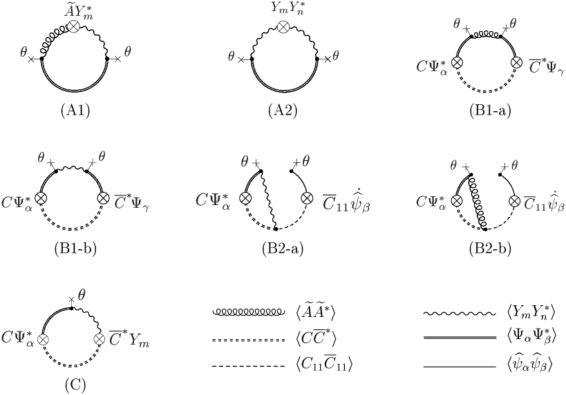
Figure 1: Schematic depiction of Feynman diagrams relevant for the calculations in this appendix.

Calculation of $\Delta_{\epsilon}\theta^{A}_{\alpha}(\tau)$:  The explicit expression is

$$\Delta\theta^{A}_{\alpha}=g^{2}\langle\widetilde{A}Y_{m}^{\ast}-Y_{m}\widetilde{A}^{\ast}\rangle(\gamma^{m}\epsilon)_{\alpha}+i{g^{2}\over 2}\langle Y_{m}Y^{\ast}_{n}-Y_{n}Y^{\ast}_{m}\rangle(\gamma^{mn}\epsilon)_{\alpha}\,.$$ (A.5)

To compute the expectation values above to ${\cal O}(\theta^{2})$, we need to perform the second order perturbation using the ${\cal O}(\theta)$ vertices

$$\widetilde{S}_{\widetilde{A}\Psi} = -i\int\!d\tau\theta_{\alpha}(\widetilde{A}\Psi_{\alpha}^{\ast}-\Psi_{\alpha}\widetilde{A}^{\ast})\,,$$ (A.6)

$$\widetilde{S}_{Y\Psi} = -\int\!d\tau(\gamma^{m}\theta)_{\alpha}(Y_{m}\Psi^{\ast}_{\alpha}-Y^{\ast}_{m}\Psi_{\alpha})\,.$$ (A.7)

This generates the diagrams (A1) and (A2) in Fig. 1, for the first and the second term in (A.5) respectively. Consider for example the term $\langle\widetilde{A}(\tau)Y_{m}^{\ast}(\tau)\rangle$. Using the tree-level propagators given in (5.64) and (5.68), this can be computed as

$$\langle\widetilde{A}(\tau)Y_{m}^{\ast}(\tau)\rangle = i\int\!d\tau^{\prime}d\tau^{\prime\prime}\langle\widetilde{A}(\tau)\widetilde{A}^{\ast}(\tau^{\prime})\rangle\theta_{\alpha}(\tau^{\prime})(\gamma^{n}\theta(\tau^{\prime\prime}))_{\beta}\langle\Psi_{\alpha}(\tau^{\prime})\Psi_{\beta}^{\ast}(\tau^{\prime\prime})\rangle$$ (A.8)

$$\qquad\times\langle Y_{n}(\tau^{\prime\prime})Y_{m}^{\ast}(\tau)\rangle$$

$$= -i\langle\tau|\Delta\theta_{\alpha}(\partial+r\!\!\!/)_{\alpha\beta}(\gamma^{m}\theta)_{\beta}\Delta^{2}|\tau\rangle\,.$$

Performing the normal-ordering, neglecting the terms which generate derivatives, this becomes

$$\langle\widetilde{A}(\tau)Y_{m}^{\ast}(\tau)\rangle=-i(\theta r\!\!\!/\gamma^{m}\theta)\langle\tau|\Delta^{3}|\tau\rangle=-{3i\over 16r^{5}}(\theta r\!\!\!/\gamma^{m}\theta)={3i\over 16r^{5}}r_{l}(\theta\gamma^{ml}\theta)\,.$$ (A.9)

Likewise, one easily finds that $-\langle\widetilde{A}^{\ast}(\tau)Y_{m}(\tau)\rangle$ gives exactly the same contribution. The evaluation of the diagram (A2) proceeds in an entirely similar manner. In this way one finds

$$\Delta\theta^{A}_{\alpha}={3ig^{2}\over 16r^{5}}\left(2r_{l}(\theta\gamma^{ml}\theta)(\gamma^{m}\epsilon)_{\alpha}-r_{l}(\theta\gamma^{mnl}\theta)(\gamma^{nm}\epsilon)_{\alpha}\right)\,.$$ (A.10)

Calculation of $\Delta_{\epsilon}\theta^{B}_{\alpha}(\tau)$:  This receives contributions from two classes of diagrams, (B1) and (B2) in Fig.1.

For (B1), we have

$$\Delta_{\epsilon}\theta^{B1}_{\alpha}(\tau) = \epsilon_{\beta}g^{2}\!\int\!d\tau^{\prime}\Biggl{(}\langle C^{\ast}(\tau)\overline{C}(\tau^{\prime})\rangle(\partial+r\!\!\!/)_{\beta\gamma}\langle\Psi^{\ast}_{\gamma}(\tau^{\prime})\Psi_{\alpha}(\tau)\rangle$$ (A.11)

$$-\langle C(\tau)\overline{C}^{\ast}(\tau^{\prime})\rangle(\partial-r\!\!\!/)_{\beta\gamma}\langle\Psi_{\gamma}(\tau^{\prime})\Psi^{\ast}_{\alpha}(\tau)\rangle\Biggr{)}\,.$$

Insertions of the vertices $\widetilde{S}_{\widetilde{A}\Psi}$ (A.6) and $\widetilde{S}_{Y\Psi}$ (A.7) twice generate the diagrams (B1-a) and (B1-b). Again neglecting the derivatives produced in the process of normal ordering we obtain

$$\Delta\theta^{B1}_{\alpha}={3ig^{2}\over 16r^{5}}\left(2(\epsilon\theta)(r\!\!\!/\theta)_{\alpha}-2(\epsilon r\!\!\!/\theta)\theta_{\alpha}-2r_{l}(\epsilon\gamma^{m}\theta)(\theta\gamma^{ml})_{\alpha}\right)\,.$$ (A.12)

Now, in distinction to all the other contributions, the one from (B2) involves propagation of massless fields $\hat{\psi}_{\alpha}$, $C_{11}$ and $\overline{C}_{11}$ in the intermediate steps. The original expression is, to the order of interest,

$$\Delta_{\epsilon}\theta^{B2}_{\alpha}=-g\epsilon_{\beta}\!\int\!d\tau^{\prime}\langle C\Psi^{\ast}(\tau)\overline{C}_{11}\dot{\widehat{\psi}\ }\mbox{}\!\!_{\beta}(\tau^{\prime})\rangle+g\epsilon_{\beta}\!\int\!d\tau^{\prime}\langle C^{\ast}\Psi(\tau)\overline{C}_{11}\dot{\widehat{\psi}}_{\beta}(\tau^{\prime})\rangle\,.$$ (A.13)

To extract ${\cal O}(\theta^{2})$ contributions, we need to use the following five types of vertices:

$$V_{1} \equiv -ig\int\!d\tau\left(r^{m}\overline{C}^{\ast}C_{11}Y^{m}+r^{m}\overline{C}Y^{m\ast}C_{11}\right)\,,$$ (A.14)

$$V_{2} \equiv \int\!d\tau\theta\gamma^{n}(\Psi Y^{m\ast}-Y^{m}\Psi^{\ast})\,,$$ (A.15)

$$V_{3} \equiv g\int\!d\tau(\overline{C}^{\ast}\dot{C}_{11}\widetilde{A}+\overline{C}^{\ast}C_{11}\dot{\widetilde{A}\ }\!-\overline{C}\dot{\widetilde{A}^{\ast}}C_{11}-\overline{C}\widetilde{A}^{\ast}\dot{C}_{11})\,,$$ (A.16)

$$V_{4} \equiv i\int\!d\tau\theta(\Psi\widetilde{A}^{\ast}-\widetilde{A}\Psi^{\ast})\,,$$ (A.17)

$$V_{5} \equiv -\frac{1}{g^{2}}\int\!d\tau{\dot{\widehat{\psi}\ }}\theta\,.$$ (A.18)

First, inserting $V_{1},V_{2}$ and $V_{5}$, we get the diagrams of the type (B2-a). This gives the contribution

$$\Delta_{\epsilon}\theta^{B2-a}_{\alpha}=2ig^{2}\!\int\!d\tau^{\prime}\ d\tau^{\prime\prime}\langle\tau|\Delta|\tau^{\prime\prime}\rangle\langle\tau^{\prime\prime}|\frac{1}{\partial}|\tau^{\prime}\rangle r^{n}(\tau^{\prime\prime})\langle\tau^{\prime\prime}|\Delta(\gamma^{n}\theta)_{\alpha}\partial\Delta|\tau\rangle(\epsilon\theta)(\tau^{\prime})\,.$$

Similarly, use of $V_{3},V_{4}$ and $V_{5}$ generates the diagrams of the type (B2-b), the contribution of which is worked out to be

$$\Delta_{\epsilon}\theta^{B2-b}_{\alpha}=2ig^{2}\langle\tau|\Delta(\epsilon\theta)\Delta r^{m}(\gamma^{m}\theta)_{\alpha}\Delta|\tau\rangle-\Delta_{\epsilon}\theta^{B2-a}_{\alpha}\,.$$ (A.20)

Therefore,

$$\Delta_{\epsilon}\theta^{B2}_{\alpha}=\Delta_{\epsilon}\theta^{B2-a}_{\alpha}+\Delta_{\epsilon}\theta^{B2-b}_{\alpha}=2ig^{2}(\epsilon\theta)\langle\tau|\Delta^{3}|\tau\rangle(r\!\!\!/\theta)_{\alpha}={3ig^{2}\over 16r^{5}}2(\epsilon\theta)(r\!\!\!/\theta)_{\alpha}\,.$$ (A.21)

Calculation of $\Delta_{\epsilon}\theta^{C}_{\alpha}(\tau)$:  Finally, consider $\Delta_{\epsilon}\theta^{C}_{\alpha}$. It takes the form

$$\Delta_{\epsilon}\theta^{C}_{\alpha}(\tau) = g^{2}\!\int\!d\tau^{\prime}\Biggl{(}\langle C(\tau)\overline{C}^{\ast}(\tau^{\prime})\rangle\langle Y_{m}(\tau^{\prime})\Psi_{\alpha}^{\ast}(\tau)\rangle$$ (A.22)

$$\qquad+\langle C^{\ast}(\tau)\overline{C}(\tau^{\prime})\rangle\langle Y^{\ast}_{m}(\tau^{\prime})\Psi_{\alpha}(\tau)\rangle\Biggr{)}\epsilon^{T}\gamma^{m}\theta(\tau^{\prime})\,,$$

which is represented by the diagram $(C)$. Using the vertex (A.7) and proceeding similarly to the previous calculations, we obtain

$$\Delta\theta^{C}_{\alpha}={3ig^{2}\over 16r^{5}}\left(-2(\epsilon r\!\!\!/\theta)\theta_{\alpha}-2r_{l}(\epsilon\gamma^{m}\theta)(\theta\gamma^{ml})_{\alpha}\right)\,.$$ (A.23)

Summary:   Adding up all the contributions and reinstating the factor of $N$, the final result is

$$\Delta_{\epsilon}\theta_{\alpha} = {3ig^{2}N\over 16r^{5}}\Biggl{(}-r_{l}(\theta\gamma^{mnl}\theta)(\gamma^{nm}\epsilon)_{\alpha}+2r_{l}(\theta\gamma^{ml}\theta)(\gamma^{m}\epsilon)_{\alpha}-4r_{l}(\epsilon\gamma^{m}\theta)(\theta\gamma^{ml})_{\alpha}$$ (A.24)

$$\qquad+4(\epsilon\theta)(r\!\!\!/\theta)_{\alpha}-4(\epsilon r\!\!\!/\theta)\theta_{\alpha}\Biggr{)}\,.$$

Appendix B:  $SO(9)$ Fierz Identities

In this appendix, we record the $SO(9)$ Fierz identities which are crucial in simplifying the ${\cal O}(\theta^{2})$ part of $\Delta_{\epsilon}\theta_{\alpha}$ at 1-loop.

Adapting the notations of Taylor and Raamsdonk[5], let us introduce the following quantities for $n=0,1,2,3$ (repeated indices are summed):

$$E_{n} = r_{m}(\epsilon\gamma^{a_{1}\cdots a_{n}m}\theta)(\theta\gamma^{a_{n}\cdots a_{1}}\lambda)\,,$$ (B.1)

$$\bar{E}_{n} = r_{m}(\epsilon\gamma^{a_{1}\cdots a_{n}}\theta)(\theta\gamma^{a_{n}\cdots a_{1}m}\lambda)\,,$$ (B.2)

$$F_{n} = r_{m}(\theta\gamma^{a_{1}\cdots a_{n}m}\theta)(\lambda\gamma^{a_{n}\cdots a_{1}}\epsilon)\,,$$ (B.3)

$$\bar{F}_{n} = r_{m}(\theta\gamma^{a_{1}\cdots a_{n}}\theta)(\lambda\gamma^{a_{n}\cdots a_{1}m}\epsilon)\,,$$ (B.4)

$$P = {1\over 4!}r_{m}\epsilon^{a_{1}a_{2}a_{3}a_{4}b_{1}b_{2}b_{3}b_{4}m}(\epsilon\gamma^{a_{1}a_{2}a_{3}a_{4}}\theta)(\theta\gamma^{b_{1}b_{2}b_{3}b_{4}m}\lambda)\,,$$ (B.5)

$$Q = {1\over 4!}r_{m}\epsilon^{a_{1}a_{2}a_{3}a_{4}b_{1}b_{2}b_{3}b_{4}m}(\theta\gamma^{a_{1}a_{2}a_{3}a_{4}}\theta)(\lambda\gamma^{b_{1}b_{2}b_{3}b_{4}m}\epsilon)\,,$$ (B.6)

where $\lambda$ is an arbitrary spinor. Because $\theta\Gamma\theta=0$ for any symmetric matrix $\Gamma$, five of them actually vanish, namely

$$F_{0}=\bar{F}_{0}=\bar{F}_{1}=F_{3}=Q=0\,.$$ (B.7)

Since there are nine independent Fierz identities[5], only four structures are independent, which we take to be $F_{1},F_{2},\bar{F}_{2}$ and $\bar{F}_{3}$. Then the remaining quantities can be expressed in terms of them as

$$E_{0} = {1\over 16}F_{1}-{1\over 32}(F_{2}+\bar{F}_{2})-{1\over 96}\bar{F}_{3}\,,$$ (B.8)

$$\bar{E}_{0} = -{1\over 16}F_{1}-{1\over 32}(F_{2}+\bar{F}_{2})+{1\over 96}\bar{F}_{3}\,,$$ (B.9)

$$E_{1} = -{3\over 8}F_{1}-{1\over 8}(F_{2}-\bar{F}_{2})-{1\over 48}\bar{F}_{3}\,,$$ (B.10)

$$\bar{E}_{1} = -{3\over 8}F_{1}+{1\over 8}(F_{2}-\bar{F}_{2})-{1\over 48}\bar{F}_{3}\,,$$ (B.11)

$$E_{2} = {7\over 4}F_{1}-{1\over 4}(F_{2}+\bar{F}_{2})+{1\over 24}\bar{F}_{3}\,,$$ (B.12)

$$\bar{E}_{2} = -{7\over 4}F_{1}-{1\over 4}(F_{2}+\bar{F}_{2})-{1\over 24}\bar{F}_{3}\,,$$ (B.13)

$$E_{3} = -{21\over 4}F_{1}+{3\over 4}(F_{2}-\bar{F}_{2})+{3\over 8}\bar{F}_{3}\,,$$ (B.14)

$$\bar{E}_{3} = -{21\over 4}F_{1}-{3\over 4}(F_{2}-\bar{F}_{2})+{3\over 8}\bar{F}_{3}\,,$$ (B.15)

$$P = {15\over 2}(F_{2}+\bar{F}_{2})\,.$$ (B.16)

¿From these relations, one easily finds the identity

$$0=F_{2}-2F_{1}-4\bar{E}_{1}+4\bar{E}_{0}+12E_{0}\,.$$

Removing $\lambda$, we get

$$0 = -r_{l}(\theta\gamma^{mnl}\theta)(\gamma^{nm}\epsilon)_{\alpha}+2r_{l}(\theta\gamma^{nl}\theta)(\gamma^{n}\epsilon)_{\alpha}+4r_{l}(\epsilon\gamma^{n}\theta)(\gamma^{nl}\theta)_{\alpha}$$ (B.17)

$$\qquad+4r_{l}(\epsilon\theta)(\gamma^{l}\theta)_{\alpha}+12r_{l}(\epsilon\gamma^{l}\theta)\theta_{\alpha}\,,$$

which was used in Sec. 5.

References

- [1] T. Banks, W. Fischler, S. H. Shenker and L. Susskind, Phys. Rev. D55 (1997) 5112, hep-th/9610043.
- [2] L. Susskind, hep-th/9704080.
- [3] Y. Okawa and T. Yoneya, Nucl. Phys. B538 (1999) 67, hep-th/9806108.
- [4] Y. Okawa and T. Yoneya, Nucl. Phys. B541 (1999) 163, hep-th/9808188.
- [5] W. Taylor and M. V. Raamsdonk, J. High Energy Phys. 04 (1999) 013, hep-th/9812239.
- [6] A. Sen, Adv. Theor. Math. Phys. 2 (1998) 51, hep-th/9709220.
- [7] N. Seiberg, Phys. Rev. Lett. 79 (1997) 3577, hep-th/9710009.
- [8] A. Jevicki and T. Yoneya, Nucl. Phys. B535 (1998) 335, hep-th/9805069.
- [9] A. Jevicki, Y. Kazama and T. Yoneya, Phys. Rev. Lett. 81 (1998) 5072, hep-th/9808039.
- [10] A. Jevicki, Y. Kazama and T. Yoneya, Phys. Rev. D59 (1999) 066001, hep-th/9810146.
- [11] J. Maldacena, Adv. Theor. Math. Phys. 2 (1998) 231, hep-th/9711200.
- [12] S. Paban, S. Sethi and M. Stern, Nucl. Phys. B534 (1998) 137, hep-th/9805018.
- [13] S. Paban, S. Sethi and M. Stern, J. High Energy Phys. 06 (1998) 012, hep-th/9806028.
- [14] D. A. Lowe, J. High Energy Phys. 11 (1998) 009, hep-th/9810075.
- [15] S. Sethi and M. Stern, J. High Energy Phys. 06 (1999) 004, hep-th/9903049.
- [16] S. Hyun, Y. Kiem and H. Shin, Nucl. Phys. B558 (1999) 349, hep-th/9903022.
- [17] H. Nicolai and J. Plefka, hep-th/0001106.
- [18] Y. Okawa, talk at YITP Workshop (Kyoto, July, 1999).
- [19] M. R. Douglas, D. Kabat, P. Pouliot and S. H. Shenker, Nucl. Phys. B485 (1997) 85, hep-th/9608024.
- [20] Y. Okawa, Nucl. Phys. B552 (1999) 447, hep-th/9903025.
- [21] H. Hata and S. Moriyama, Phys. Lett. B452 (1999) 45, hep-th/9901034.
- [22] B. de Wit and D. Z. Freedman, Phys. Rev. D12 (1975) 2286.
- [23] H. Hata and S. Moriyama, Phys. Rev. D60 (1999) 126006, hep-th/9904042.