SUNY-NTG-00/03

Chiral Random Matrix Model for Critical Statistics

A.M. Garcia-Garcia and J.J.M. Verbaarschot

Department of Physics and Astronomy, SUNY, Stony Brook, New York 11794

Abstract

We propose a random matrix model that interpolates between the chiral random matrix ensembles and the chiral Poisson ensemble. By mapping this model on a non-interacting Fermi-gas we show that for energy differences less than a critical energy $E_{c}$ the spectral correlations are given by chiral Random Matrix Theory whereas for energy differences larger than $E_{c}$ the number variance shows a linear dependence on the energy difference with a slope that depends on the parameters of the model. If the parameters are scaled such that the slope remains fixed in the thermodynamic limit, this model provides a description of QCD Dirac spectra in the universality class of critical statistics. In this way a good description of QCD Dirac spectra for gauge field configurations given by a liquid of instantons is obtained.

PACS: 11.30.Rd, 12.39.Fe, 12.38.Lg, 71.30.+h
Keywords: QCD Dirac Spectra; Spectral Correlations; Critical Statistics; Fermi-Gas Method.

1 Introduction

By now it has been well-established that the smallest eigenvalues of the QCD Dirac operator are correlated according to a Random Matrix Theory with the global symmetries of the QCD partition function [1] (see [2, 3] for recent reviews and a complete list of references). In particular, this has been confirmed by the analysis of the low-energy effective theory [4, 5, 6, 7], universality studies [8, 9, 10, 11, 12], lattice QCD simulations [13, 4, 14, 15, 17, 18, 16, 19, 20, 21, 22] and the study two-sublattice theories with disorder [23, 24, 25, 26]. This means that the dynamical details of QCD are not important on energy scales of the order of the average level spacing. The natural question that can be asked is at what energy scale the dynamics of QCD becomes relevant and how does this manifest itself in the Dirac spectrum.

The answer to this question has been understood within the context of effective theories [27, 28, 4, 5, 6, 7]. The effective theory for the QCD Dirac spectrum is known as the partially quenched effective partition function and was originally introduced to study the quenched approximation in QCD [29, 30]. The central observation is that in the domain where the mass dependence of the effective partition function is given by the contribution of the constant fields (the zero momentum modes) the Dirac eigenvalues are correlated according to chiral Random Matrix Theory. The relevant mass scale can thus be identified as the scale for which the Compton wavelength of the lightest particle becomes equal to the size of the box i.e., $M\sim 1/L_{s}$. In QCD, in the phase of spontaneously broken chiral symmetry, the lightest particles are the Goldstone modes with a mass given by $M^{2}\sim Km$ (with $m$ the quark mass and $K=\Sigma/F^{2}$ in terms of the pion decay constant $F$ and the chiral condensate $\Sigma$). The critical scale is thus given by [4]

$$E_{c}=\frac{1}{KL^{2}_{s}}.$$ (1)

In the context of disordered condensed matter systems [31, 32, 33] this energy scale is known as the Thouless energy and also in this article we will adopt this name.

A more intuitive interpretation of the Thouless energy has been given in the theory of mesoscopic systems [31]. The time scale $\hbar/E_{c}$ is the time for which an initially localized wave packet diffuses all over space. For this reason the eigenvalues are correlated according to Random Matrix Theory for energy differences below $E_{c}$ (known as the ergodic regime). At shorter time scales, different wave functions do not necessarily overlap resulting in a weakening of correlations of the corresponding eigenvalues. For energy differences beyond the inverse elastic collision time $\tau_{e}$ the corresponding eigenvalues are completely uncorrelated (the Poisson ensemble). The domain inbetween $E_{c}$ and $\hbar/\tau_{e}$ is known as the diffusive or Altshuler-Shklovskii domain. A third energy scale is the average level spacing $\Delta\lambda$. The ratio $E_{c}/\Delta\lambda$ is identified in mesoscopic physics as the dimensionless conductance. It is equal to the number of subsequent levels correlated according to Random Matrix Theory. The existence of these domains has been confirmed by numerical simulations of the Anderson model [34].

In QCD the average level spacing is related to the order parameter of the chiral phase transition, the chiral condensate, by the Banks-Casher formula [35] according to $\Delta\lambda=\pi/\Sigma V$ (with $V$ the volume of Euclidean space-time). The prediction from (1) is that the number of eigenvalues correlated according to chRMT is of the order $F^{2}\sqrt{V}$.

For increasing disorder the number of subsequent eigenvalues described by Random Matrix Theory decreases. For strong disorder we expect that all states become localized with uncorrelated eigenvalues. We thus expect a critical value of the disorder for which the three scales, $\Delta\lambda$, $E_{c}$ and $\hbar/\tau_{e}$ coincide. In particular, the dimensionless conductance becomes volume independent [36]. It has been conjectured [37] that at this point the eigenvalue correlations are described by a new universality class known as critical statistics (see [38] for a review). In this class, only the short range correlations of the eigenvalues are described by the usual random matrix ensembles whereas the number variance, $\Sigma^{2}(n)$, shows a linear $n$-dependence beyond this domain. What is relevant for QCD is that such behavior has been observed in numerical simulations of the 4-dimensional Anderson model [39].

The volume dependence of the Thouless energy has been investigated by means of lattice QCD simulations [16, 18, 22] and instanton-liquid simulations [5]. In essence, results from lattice QCD simulations are in complete agreement with theoretical results from partial quenched chiral perturbation theory. However, the results from instanton liquid simulations seem to deviate from the prediction (1) with a scale independent constant $K$; in that case the Thouless energy only shows a weak volume dependence. This raises the question whether the Dirac eigenvalues might be described by critical statistics. To address this issue we generalize a random matrix model for critical statistics [40, 41] to include the chiral symmetry of the QCD partition function (section 2). In section 3 we map our model on a partition function of noninteracting fermions. This model is solved in the semi-classical limit in section 4, where we obtain analytical expressions for the microscopic spectral density and the two-point correlation function. Comparisons with instanton simulations are shown in section 5 and concluding remarks are made in section 6.

2 Definition of the Model

The random matrix model of Moshe and Neuberger and Shapiro [40] is defined by the partition function

$$Z=\int dHe^{-{\rm Tr}HH^{\dagger}}\int dUe^{-b{\rm Tr}([U,H][U,H]^{\dagger})},$$ (2)

where $H$ is a Hermitian and $U$ a Unitary $N\times N$ matrix. The integration measures $dH$ and $dU$ are given by the Haar measure. This model can be interpreted as the zero-dimensional limit of the Kazakov-Migdal model [42]. It interpolates between the Gaussian Unitary Ensemble $(b=0$) and the Poisson Ensemble $(b\to\infty)$. Using the invariance of the measure, the integral over $U$ can be replaced by an integral over the eigenvalues of $U$. For $b\rightarrow\infty$ this partition function is dominated by matrices $H$ that commute with arbitrary diagonal unitary matrices. This set of matrices is the ensemble of diagonal Hermitian matrices which is known as the Poisson ensemble. What is nice about this model is that it preserves the unitary invariance which enables us to take full advantage of the existing random matrix theory methods. In order to obtain a nontrivial $b$-dependence in the thermodynamic limit, the parameter $b$ has to be scaled as

$$b=h^{2}N^{2}.$$ (3)

It has been shown that in this limit the model (2) is equivalent [41] to both a banded random matrix model [43] with a power-like cutoff [44] and to random matrix models with a ${\rm Tr}\log^{2}H$ probability potential [45]. The correlation functions of the latter model have been derived by means of $q$-orthogonal polynomials [45, 46] and Painlevé equations [47].

In this paper we are interested in chiral random matrix ensembles defined as ensembles of $N\times N$ random matrices with the structure

$$D=\left(\begin{array}[]{cc}0&C\\ C^{\dagger}&0\end{array}\right),$$ (6)

where $C$ is an arbitrary complex matrix $n\times(n+\nu)$ matrix ($N=2n+\nu$). Since the matrix $D$ has exactly $\nu$ zero eigenvalues $\nu$ is interpreted as the topological quantum number. The chiral Gaussian Unitary Ensemble (chGUE) with $N_{f}$ flavors is defined as the ensemble of matrices $D$ with matrix elements $C$ distributed according to the Gaussian probability distribution

$$P(C)\sim{\det}^{N_{f}}(D+m)e^{-N{\rm Tr}CC^{\dagger}}.$$ (7)

Here, for simplicity we have taken all quark masses equal to $m$. The probability distribution $P(C)$ has the unitary invariance

$$C\rightarrow UCV^{-1},$$ (8)

where $U$ and $V$ are unitary matrices. Since an arbitrary complex matrix can always be brought to diagonal form by this transformation this invariance allows us to factorize the probability distribution in a product over the eigenvalues of $C$ and the unitary matrices that diagonalize $C$.

The generalization of the model of Moshe, Neuberger and Shapiro to the chiral ensembles is immediate. The interpolating model is defined by the partition function

$$Z_{\nu}=\int dC{\det}^{N_{f}}(D+m)e^{-\frac{\Sigma^{2}}{4h}{\rm Tr}D^{\dagger}D}\int d{\cal U}e^{-\frac{\Sigma^{2}hN^{2}}{4}{\rm Tr}[D,{\cal U}][D,{\cal U}]^{\dagger}},$$ (9)

where ${\cal U}$ has the chiral block structure

$${\cal U}=\left(\begin{array}[]{cc}U&0\\ 0&V\end{array}\right),$$ (12)

with $U$ an $n\times n$ unitary matrix and $V$ an $(n+\nu)\times(n+\nu)$ unitary matrix. If $\Sigma$ and $h$ are constants as in (9) we will refer to this model as the critical chiral unitary ensemble. As we will see below, in order to make contact with the Thouless energy in the partially quenched effective partition function we have to scale $h$ with an additional factor $1/\sqrt{N}$. The unitary invariance of this partition function follows from the invariance of the Haar measure. In comparison to [40], an additional factor $\sim\Sigma^{2}/h$ has been included in the probability distribution of the matrix elements. As we will see below, this will guarantee that in the thermodynamic limit the spectral density is $h$-independent to leading order in $h$. We will also find that the partition function is normalized such that the $\Sigma$ represents the chiral condensate by means of the Banks-Casher relation $\Sigma=\pi\rho(0)/N$ (with $\rho(0)$ the spectral density around $\lambda=0$).

Decomposing into the blocks of $D$ and ${\cal U}$ the partition function can be written as

$$Z_{\nu}=m^{\nu}\int dC{\det}^{N_{f}}[C^{\dagger}C+m^{2}]e^{-(1+2h^{2}N^{2})\frac{\Sigma^{2}}{2h}{\rm Tr}CC^{\dagger}}\int dUdVe^{\Sigma^{2}hN^{2}{\rm Re}{\rm Tr}UCV^{-1}C^{\dagger}}.$$ (13)

The arbitrary complex matrix $C$ can be decomposed according to

$$C=U_{1}\Lambda U_{2},$$ (14)

and the integral over $C$ can be expressed as an integral over the eigenvalues $\Lambda_{k}$ and the unitary matrices $U_{1}$ and $U_{2}$. Up to a irrelevant constant, the Jacobian of this transformation is given by

$$J(\Lambda)=\Delta^{2}(\{\lambda_{i}^{2}\})\prod_{k}\lambda_{k}^{2\nu+1}.$$ (15)

where

$$\Delta(\{\lambda_{i}^{2}\})=\prod_{k<l}(\lambda_{k}^{2}-\lambda_{l}^{2})$$ (16)

is the Vandermonde determinant. Because of the unitary invariance, the $U_{1}$ and $U_{2}$ dependence in the second exponent can be absorbed in a redefinition of $U$and $V$, and the integrations over $U_{1}$ and $U_{2}$ just result in an overall constant. Remarkably, the integral over $U$ and $V$ in (13) is an Itzykson-Zuber type integral which is known analytically [48, 49, 50]

$$\int dUdVe^{z{\rm Re}{\rm Tr}U\Lambda V^{-1}\Lambda}=C\frac{\det_{k,l}\left|I_{\nu}(z\lambda_{k}\lambda_{l})\right|}{\Delta^{2}(\{\lambda_{i}^{2}\})\prod_{k=1}^{n}\lambda_{k}^{2\nu}}.$$ (17)

The Vandermonde determinants cancel resulting in the partition function

$$Z_{\nu}=m^{\nu}\int\prod_{k=1}^{n}d\lambda_{k}\prod_{k=1}^{n}(\lambda_{k}^{2}+m^{2})^{N_{f}}\det_{k,l}\left|(\lambda_{k}\lambda_{l})^{\frac{1}{2}}e^{-(\frac{1}{2}+h^{2}N^{2})\frac{\Sigma^{2}}{2h}(\lambda_{k}^{2}+\lambda_{l}^{2})}I_{\nu}(h\Sigma^{2}N^{2}\lambda_{k}\lambda_{l})\right|.$$

(18)

The instanton-liquid Dirac spectra that will be described by this model were obtained in the quenched approximation and for zero total topological charge. Therefore we will not attempt to solve this model for arbitrary $N_{f}$ but instead focus on the technically simpler case of $N_{f}=0$. Since the topological charge does not give rise to additional complications we will consider the case of arbitrary $\nu$. Below we will thus analyze the joint probability distribution

$$\rho_{\nu}(\lambda_{1},\cdots,\lambda_{n})\equiv\det_{k,l}\left|(\lambda_{k}\lambda_{l})^{\frac{1}{2}}e^{-(\frac{1}{2}+h^{2}N^{2})\frac{\Sigma^{2}}{2h}(\lambda_{k}^{2}+\lambda_{l}^{2})}I_{\nu}(h\Sigma^{2}N^{2}\lambda_{k}\lambda_{l})\right|.$$

(19)

3 Fermi-Gas Representation of the Interpolating chiral Random Matrix Model

In this section we rewrite the joint probability distribution (19) in terms of the fermionic $n$-particle matrix element

$$\rho_{\nu}(x_{1},\cdots,x_{n})\equiv C\langle x_{1}\cdots x_{n}|e^{-\beta H}|x_{1}\cdots x_{n}\rangle,$$ (20)

where $H$ is the separable Hamiltonian

$$H=\sum_{k}(-\partial_{k}^{2}+\frac{4\nu^{2}-1}{4x^{2}_{k}}+\omega^{2}x_{k}^{2}),$$ (21)

and $C$ is an irrelevant constant. The eigenfunctions of the single particle Hamiltonian are known in terms of Laguerre polynomials. Specifically,

$$(-\partial_{x}^{2}+\frac{4\nu^{2}-1}{4x^{2}}+\omega^{2}x^{2})\phi_{n}=\omega_{n}\phi_{n},$$ (22)

has the solutions

$$\omega_{n} = (4n+2\nu+2)\omega,$$ (23)

$$\phi_{n} = \frac{\sqrt{2}\omega^{1/4}}{\sqrt{h}_{n}}e^{-\omega x^{2}/2}\left(x\sqrt{\omega}\right)^{\nu+\frac{1}{2}}L_{n}^{\nu}\left({x^{2}}\omega\right).$$ (24)

The normalization factor $h_{n}=(n+\nu)!/n!$ ensures that the $\phi_{n}$ are normalized to unity

$$\int_{0}^{\infty}\phi_{n}(x)\phi_{n}(x)dx=1.$$ (25)

Using completeness, the many-particle matrix element can be written as

$$\langle x_{1}\cdots x_{n}|e^{-\beta H}|x_{1}\cdots x_{n}\rangle=\det_{ij}\sum_{n}\phi_{n}(x_{i})e^{-\beta\omega_{n}}\phi_{n}(x_{j})$$ (26)

The sum over $n$ can be performed analytically using the identity

$$\sum_{n=0}^{\infty}\frac{L_{n}^{\nu}(x)L_{n}^{\nu}(y)z^{n}}{h_{n}}=\frac{(xyz)^{-\nu/2}}{1-z}\exp\left(-z\frac{x+y}{1-z}\right)I_{\nu}\left(\frac{2\sqrt{xyz}}{1-z}\right).$$ (27)

With $z=\exp(-4\beta\omega)$ this results in

$$\langle x_{1}\cdots x_{n}|e^{-\beta H}|x_{1}\cdots x_{n}\rangle=\det_{ij}\left|\frac{\omega\sqrt{x_{i}x_{j}}}{\sinh 2\beta\omega}\exp\left(-\frac{\omega\cosh 2\beta\omega}{2\sinh 2\beta\omega}(x^{2}_{i}+x^{2}_{j})\right)I_{\nu}\left(\frac{\omega}{\sinh 2\beta\omega}x_{i}x_{j}\right)\right|.$$

Comparing this expression with (19) we find that

$$\omega = \sqrt{4h^{2}N^{2}+1}\frac{\Sigma^{2}}{2h},$$ (29)

$$\cosh 2\beta\omega = 1+\frac{1}{2h^{2}N^{2}}.$$ (30)

The joint probability distribution of the eigenvalues is thus given by an $n-$particle diagonal matrix element of the density operator. The average spectral density is equal to the average particle density. It is obtained by integrating over the positions of all particles except one. The integral can be performed by rewriting the matrix elements (26) in terms of a sum over permutations $\pi$ and $\pi^{\prime}$,

$$\frac{1}{n!}\sum_{\omega_{1}<\cdots<\omega_{n}}\sum_{\pi\pi^{\prime}}\sigma(\pi)\sigma(\pi^{\prime})\phi_{\omega_{\pi(1)}}(x_{1})\cdots\phi_{\omega_{\pi(n)}}(x_{n})e^{-\beta\sum_{k}\omega_{k}}\phi_{\omega_{\pi^{\prime}(1)}}(x_{1})\cdots\phi_{\omega_{\pi^{\prime}(n)}}(x_{n}),$$ (31)

where $\sigma(\cdot)$ is the sign of the permutation. Performing the integrations over $x_{2},\cdots,x_{n}$, by orthogonality we find that the only nonzero contribution is for $\pi=\pi^{\prime}$. Then the remaining sum over $\pi(\omega_{1})$ is just a sum over $\omega_{1},\cdots,\omega_{n}$. For the canonical ensemble we thus find the one-particle density,

$$\langle\rho(x)\rangle\equiv\langle\sum_{k}\delta(x-x_{k})\rangle=\frac{1}{Z_{n}}\sum_{\omega_{1}<\cdots<\omega_{N}}\sum_{i}|\phi_{\omega_{i}}(x_{1})|^{2}e^{-\beta\sum_{k}\omega_{k}}.$$ (32)

In an occupation number representation this can be rewritten as

$$\langle\rho(x)\rangle=\frac{1}{Z_{n}}\sum_{\sum_{i}n_{i}=n}\sum_{i}n_{i}|\phi_{\omega_{i}}(x)|^{2}e^{-\beta\sum_{k}n_{i}\omega_{k}},$$ (33)

where the sum is over all $n_{i}\in\{0,\,1\}$ subject to the condition given below the summation sign and the canonical partition function is given by

$$Z_{n}=\sum_{\sum_{i}n_{i}=n}e^{-\beta\sum_{i}n_{i}\omega_{i}}.$$ (34)

For completeness we give the following exact expressions for the canonical partition function [51, 52]

$$Z_{n}=\frac{e^{-2\beta\omega n^{2}-2\beta\nu\omega n}}{(1-e^{-4\beta\omega})(1-e^{-8\beta\omega})\cdots(1-e^{-4n\beta\omega})},$$ (35)

and the one-particle density

$$\langle\rho(x)\rangle=\sum_{k}|\phi_{k}(x)|^{2}\sum_{r=0}^{\infty}(-1)^{r}e^{-4\beta\omega(kr-nr+\frac{1}{2}r(r+1))}\prod_{p=N-r}^{N}(1-e^{-4\beta\omega p}).$$ (36)

They have been obtained by writing the constraint $\sum_{i}n_{i}=n$ as

$$\delta(N-\sum_{i}n_{i})=\frac{1}{2\pi}\int d\theta e^{i\theta(N-\sum_{i}n_{i})},$$ (37)

and summing the geometric series after using the explicit expression (24) for the $\omega_{n}$.

Instead of working with the canonical ensemble we eliminate the constraint on the sum over the $n_{i}$ by working with the grand canonical ensemble. The grand canonical partition function is defined by

$$Z=\sum_{n}z^{n}Z_{n}=\prod_{k}(1+e^{-\beta\omega_{k}+\beta\mu}),$$ (38)

where $z=e^{\beta\mu}$ is the fugacity. The one particle density in the grand canonical ensemble is given by

$$\langle\rho(x)\rangle = \frac{1}{Z}\sum_{n}z^{n}Z_{n}\rho(x)$$ (39)

$$= \frac{1}{Z}\sum_{n_{i}\in\{0,1\}}\sum_{i}n_{i}|\phi_{i}(x)|^{2}e^{-\beta\sum_{k}n_{k}(\omega_{k}-\mu)},$$

which can be evaluated to be

$$\langle\rho(x)\rangle=\sum_{i}|\phi_{i}(x)|^{2}\frac{1}{1+e^{\beta(\omega_{i}-\mu)}}.$$ (40)

The fugacity $z=e^{\beta\mu}$ is determined by the condition that the total number of particles is equal to $n$, i.e.

$$\sum_{i}\frac{1}{1+e^{\beta(\omega_{i}-\mu)}}=n.$$ (41)

The connected two-particle correlation function is defined by

$$R_{2}(x,y)=\sum_{k\neq l}\langle\delta(x-x_{k})\delta(y-y_{l})\rangle-\langle\rho(x)\rangle\langle\rho(y)\rangle$$ (42)

It can be obtained from the $n$-particle matrix element (20) by integration over all coordinates (eigenvalues) except $x_{1}$ and $x_{2}$. The remaining sum over $\omega_{\pi(1)}$ and $\omega_{\pi(2)}$ can be rewritten as

$$\sum_{\omega_{1}<\cdots<\omega_{N}}\sum_{i\neq j}\phi_{\omega_{i}}(x_{1})\phi_{\omega_{j}}(x_{2})\left[\phi_{\omega_{i}}(x_{1})\phi_{\omega_{j}}(x_{2})-\phi_{\omega_{j}}(x_{1})\phi_{\omega_{i}}(x_{2})\right]e^{-\beta\sum_{k}\omega_{k}}.$$ (43)

The diagonal term, $i=j$, is zero allowing us to include it in the summation. The first term can then be identified as the square of the average particle density. It is the disconnected contribution to the two-particle correlation function. The connected part of the two-particle distribution function can thus be written as

$$R_{2}(x_{1},x_{2})=-\frac{1}{Z_{n}}\sum_{\omega_{1}<\cdots<\omega_{n}}\sum_{i,j}\phi_{\omega_{i}}(x_{1})\phi_{\omega_{j}}(x_{2})\phi_{\omega_{j}}(x_{1})\phi_{\omega_{i}}(x_{2})e^{-\beta\sum_{i}\omega_{i}}.$$ (44)

This correlation function does not include the contributions from the self-correlations of the eigenvalues. After all, our starting point was the joint distribution of different eigenvalues. In an occupation number representation $R_{2}(x_{1},x_{2})$ simplifies to

$$R_{2}(x_{1},x_{2})=-\frac{1}{Z_{n}}\sum_{n_{1}+n_{2}+\cdots=n}\left[\sum_{i}n_{i}\phi_{\omega_{i}}(x_{1})\phi_{\omega_{i}}(x_{2})\right]^{2}e^{-\beta\sum_{k}n_{k}\omega_{l}}.$$ (45)

Using this representation, the two-particle density in the grand canonical ensemble is found to be

$$R_{2}(x,y)=-\left|\sum_{i}\phi_{i}(x)\phi_{i}(y)\frac{1}{1+e^{\beta(\omega_{i}-\mu)}}\right|^{2}.$$ (46)

Using similar manipulations as for the canonical partition function and the corresponding one-particle density it is possible to simplify the exact analytical expression for the connected two-particle correlation function in the canonical ensemble,

$$R_{2}(x,y)=-\sum_{k,l}|\phi_{k}(x)\phi_{l}(y)|^{2}\sum_{r,s=0}^{\infty}(-1)^{r}e^{-4\beta\omega(kr+ls-n(r+s)+\frac{1}{2}(r+s)(r+s+1))}\prod_{p=N-r-s}^{N}(1-q^{p}).$$

This result can be used to compare the two ensembles but we will not address this question in this article.

4 Semiclassical Calculation

In this section we calculate the microscopic spectral density and the two-point correlation function using semi-classical methods starting from the expressions for the grand canonical ensemble derived in previous section. We are thus interested in the region around $x=0$. Because of the hard edge at $x=0$ we cannot simply do a WKB approximation by replacing the wave functions by plane waves but instead have to use Bessel functions. This follows immediately from the wave equation for $x\to 0$,

$$\left[-\partial_{x}^{2}+\frac{4\nu^{2}-1}{4x^{2}}\right]\sqrt{x}J_{\nu}(kx)=k^{2}\sqrt{x}J_{\nu}(kx).$$ (48)

Alternatively, one can exploit the asymptotic relation between Laguerre polynomials and Bessel functions.

4.1 The Microscopic Spectral Density

Taking into account the normalization of the Bessel functions, $\int_{0}^{\infty}kdk\sqrt{xx^{\prime}}J_{\nu}(kx)J_{\nu}(kx^{\prime})=\delta(x-x^{\prime})$, to fix the constants in the integration measure, we arrive at the following expression for the single particle density

$$\langle\rho(x)\rangle=\int_{0}^{\infty}kxdk\frac{J_{\nu}^{2}(kx)}{1+e^{\beta k^{2}-\beta\mu+\beta\omega^{2}x^{2}}}.$$ (49)

The chemical potential is determined by the condition $\int dx\rho(x)=n$. Since this integral is over all $x$, the use of the semi-classical expressions for the wave functions is not justified but instead we have to rely on the exact wave functions. In the limit, $\beta\mu\gg\omega$, the sum over $i$ in (41) can be replaced be an integral which can be performed analytically resulting in

$$e^{(2\nu+2)\beta\omega-\beta\mu}=\frac{1}{e^{4n\beta\omega}-1}.$$ (50)

In the limit $n\beta\omega\gg 1$ the semi-classical expression for the spectral density is thus given by

$$\langle\rho(x)\rangle=\int_{0}^{\infty}kxdk\frac{J_{\nu}^{2}(kx)}{1+e^{\beta k^{2}+\beta\omega^{2}x^{2}-(4n-2\nu-2)\beta\omega}}.$$ (51)

In this limit the semiclassical expression (49) leads to the correct value of the chemical potential. Below we will show for $n\beta\omega\gg 1$ and finite $x$ (in units of the average level spacing) the term $\beta\omega^{2}x^{2}$ can be neglected relative to $4n\beta\omega$.

An estimate for the average spectral density near zero but many level spacings away from $x=0$ is obtained by using the leading order asymptotic expansion of the Bessel functions and calculating the integral in (51) in the limit of a degenerate Fermi-gas. This results in

$$\bar{\rho}=\frac{\bar{k}}{\pi},$$ (52)

where $\bar{k}\approx\sqrt{4n\omega}$ is the “radius”of the Fermi-sphere. At fixed $h$ in the limit $n\gg 1$ we have

$$\omega\approx\Sigma^{2}n\qquad{\rm and}\qquad\beta\omega\approx\frac{1}{2hn}.$$ (53)

Using these results and invoking the Banks-Casher formula the parameter $\Sigma$ can be identified as the chiral condensate,

$$\lim_{n\rightarrow\infty}\frac{\pi\bar{\rho}}{2n}=\Sigma.$$ (54)

We will now show that our approximations are self-consistent. The condition that we are close to the degenerate Fermi gas can be written as $\delta k/\bar{k}\ll 1$. We thus have to impose the requirement that

$$\frac{\delta k}{\bar{k}}\sim\frac{1}{2\beta{\bar{k}}^{2}}=\frac{h}{4}\ll 1.$$ (55)

The conditions $kx\gg 1$ and $\beta\omega^{2}x^{2}\ll 4n\beta\omega$ can be combined into

$$\frac{1}{4n}\ll\omega x^{2}\ll 4n,$$ (56)

or, in units of the average level spacing, $x=u/\bar{\rho}$, the range of validity of the above asymptotic results is given by

$$\frac{1}{4n}\ll\frac{u^{2}\pi^{2}}{4n}\ll 4n.$$ (57)

Because of the second inequality it is justified to neglect the term $\beta\omega^{2}x^{2}$ which we will do in the remainder of this section.

By partial integration the expression (51) for the spectral density can be rewritten as

$$\langle\rho(x)\rangle=\int_{0}^{\infty}dk\frac{\beta xk^{3}\left[J_{\nu}^{2}(kx)-J_{\nu+1}(kx)J_{\nu-1}(kx)\right]}{4\cosh^{2}\frac{\beta}{2}(k^{2}-4n\omega)}.$$ (58)

Using the Banks-Casher formula one finds that the chiral condensate depends on $h$. The leading order correction is given by

$$\frac{\Sigma(h)}{\Sigma}=1-\frac{{\pi}^{2}}{96}h^{2}+\cdots.$$ (59)

The corresponding spectral density will be denoted by $\bar{\rho}(h)\equiv 2n\Sigma(h)/\pi$. The microscopic spectral density is then given by

$$\rho_{s}(u) = \lim_{n\rightarrow\infty}\frac{1}{2n\Sigma(h)}\rho(\frac{u}{2n\Sigma(h)}),$$ (60)

$$= \frac{\Sigma}{\Sigma(h)}\int_{0}^{\infty}dk\frac{k^{2}\rho_{s}^{0}(ku\Sigma/\Sigma(h))}{h\cosh^{2}\frac{(k^{2}-1)}{h}}.$$

where $\rho_{s}^{0}$ is the microscopic spectral density for the chGUE [53, 54]

$$\rho_{s}^{0}(u)=\frac{u}{2}\left[J_{\nu}^{2}(u)-J_{\nu+1}(u)J_{\nu-1}(u)\right].$$ (61)

The interpretation is clear. The oscillations in the microscopic spectral density due to the Bessel functions are smeared out over a distance $hu$ by the integration over $k$. The oscillations are thus visible up to a distance of $u\sim 1/h$.

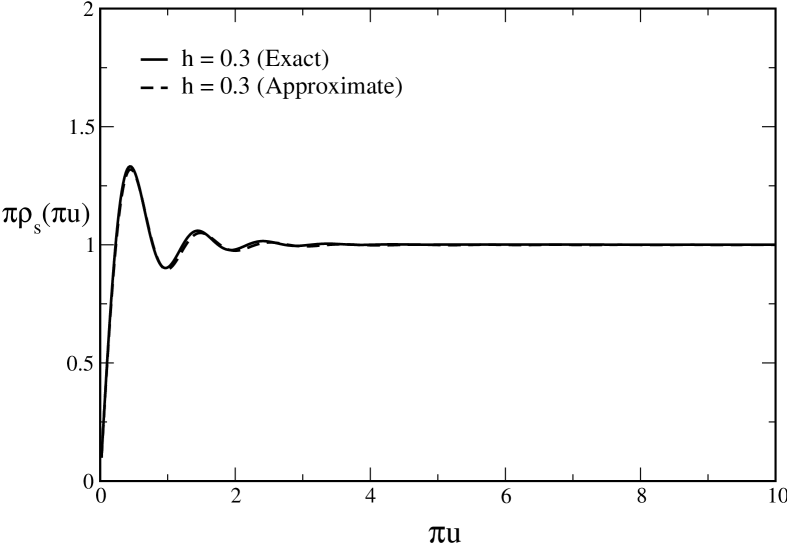
Figure 1: The microscopic spectral density $\pi\rho_{s}(\pi u)$ versus $\pi u$ for a value of $h=0.3$. The exact result (full curve) and the approximate result (dashed curve) nearly coincide.

In the limit of small $h$ the main contribution to the integral comes from the region around the Fermi-surface. In this limit we can derive an approximate formula correct to order $h^{2}$ at fixed $uh$. To this end we change integration variables in (60) according to $k=1+ht$ neglecting terms that are sub-leading in $h$. This results in

$$\rho_{s}(u)=\int_{-\infty}^{\infty}dt\frac{\rho_{s}^{0}(u+hut)}{\cosh^{2}(2t)}.$$ (62)

Next we Taylor expand the microscopic spectral density as follows

$$\rho_{s}^{0}(u+hut) = \rho_{s}^{0}(u)$$ (63)

$$+ \frac{1}{2}hut\left[J_{\nu}^{2}+J_{\nu+1}J_{\nu-1})\right]$$

$$+ \frac{1}{2}\frac{(hut)^{2}}{2!}\left[4J_{\nu}J_{\nu-1}+\frac{f_{1}}{u}\right]$$

$$+ \frac{1}{2}\frac{(hut)^{3}}{3!}\left[4(J_{\nu-1}^{2}-J_{\nu+1}^{2})+\frac{g_{1}}{u}+\frac{g_{2}}{u^{2}})\right]$$

$$+ \frac{1}{2}\frac{(hut)^{4}}{4!}\left[-4^{2}{J_{\nu}J_{\nu-1}}+\frac{h_{1}}{u^{1}}+\frac{h_{2}}{u^{2}}+\frac{h_{3}}{u^{3}})\right],$$

where the terms that will be neglected are denoted by $f_{i}$, $g_{i}$, $h_{i}$, etc.. At small values of $u$ these terms are of order $h^{2}u$ whereas for large $u$ they are suppressed by order $1/u^{2}$ (notice the factor $u$ in (61)). By inspection one easily finds that the neglected terms are at most of order $h^{2}$ independent of the value of $u$. The leading order terms can be easily resummed to

$$\rho_{s}^{0}(u+hut)=\rho_{s}^{0}(u)-\frac{1}{2}J_{\nu}(u)J_{\nu-1}(u)[\cos(2hut)-1]+O(h^{2})+\,\,\,{\rm terms\,\,odd\,\,in\,\,}t.$$ (64)

The integral over $t$ in (62) can be performed analytically resulting in

$$\rho_{s}(u)=\rho_{s}^{0}(u)-\frac{1}{2}J_{\nu}(u)J_{\nu-1}(u)\left[\frac{\pi hu}{2\sinh(\pi hu/2)}-1\right]+O(h^{2}).$$ (65)

In Fig. 1 we compare the exact expression for the microscopic spectral density (60) to this approximate formula. We observe that even for a value of $h$ as large as $h=0.3$ the two results are very close.

4.2 Two-Point Function

In this subsection we derive a semi-classical expression for the two-point correlation function. To this end the wave functions in the expression (46) for the connected two-point correlation function are replaced by Bessel functions,

$$R_{2}(x,y)=-\left|\int_{0}^{\infty}kdk\frac{\sqrt{xy}J_{\nu}(kx)J_{\nu}(ky)}{1+e^{\beta k^{2}-4n\beta\omega}}\right|^{2}.$$ (66)

By partial integration with respect to $k$ the correlation function can be expressed as

$$R_{2}(x,y)=-\left|\frac{\bar{\rho}}{h}\int_{0}^{\infty}k^{2}dk\frac{K(x\pi\bar{\rho}k,y\pi\bar{\rho}k)}{\cosh^{2}((k^{2}-1)/h)}\right|^{2},$$ (67)

where $K(x,y)$ is the two-point kernel for the chGUE given by [53, 54]

$$K(x,y)=\sqrt{xy}\frac{xJ_{\nu+1}(x)J_{\nu}(y)-yJ_{\nu}(x)J_{\nu+1}(y)}{x^{2}-y^{2}}.$$ (68)

To order $h^{2}$ the correlation function can be simplified to

$$R_{2}(x,y)=-\left|{\bar{\rho}}\int_{-\infty}^{\infty}dt\frac{K(x\pi\bar{\rho}(1+ht),y\pi\bar{\rho}(1+ht)}{\cosh^{2}2t}\right|^{2}+O(h^{2}),$$ (69)

In the same way as for the one-point function we now will derive an approximate formula for the two-point function correct to order $h^{2}$ at fixed value of $uh$. This can be done conveniently by using the following summation formula

$$J_{\nu+1}(x+xh)J_{\nu}(y+yh) \pm J_{\nu}(x+xh)J_{\nu+1}(y+yh)$$ (70)

$$\approx [J_{\nu+1}(x)J_{\nu}(y)\pm J_{\nu}(x)J_{\nu+1}(y)]\cos[(x+y)h]$$

$$+ [J_{\nu}(x)J_{\nu}(y)\mp J_{\nu+1}(x)J_{\nu+1}(y)]\sin[(x+y)h].$$

This formula has been derived by means of a Taylor expansion and a subsequent resummation employing the following approximate derivative formulas

$$\partial^{2n}_{k}[J_{\nu+1}(kx)J_{\nu}(ky) \pm J_{\nu}(kx)J_{\nu+1}(ky)]$$ (71)

$$\approx (-1)^{n}(x\pm y)^{2n}[J_{\nu+1}(kx)J_{\nu}(ky)\pm J_{\nu}(kx)J_{\nu+1}(ky)],$$

and

$$\partial^{2n-1}_{k}[J_{\nu+1}(kx)J_{\nu}(ky) \pm J_{\nu+1}(kx)J_{\nu}(ky)]$$ (72)

$$\approx (-1)^{n+1}(x\pm y)^{2n-1}[J_{\nu}(x)J_{\nu}(y)\mp J_{\nu+1}(x)J_{\nu+1}(y)].$$

They have been obtained by means of recursion relations for Bessel functions neglecting terms that are suppressed by order $1/x$ or $1/y$. One can easily show that the combined powers of $x$ and $y$ in the prefactor is always larger than the combined powers of $x$ and $y$ that have been neglected. Since only even terms in $t$ contribute to the integral in (69) our final result for the two-point function, correct to order $h^{2}$, is given by

$$R_{2}(x,y)= -\bar{\rho}^{2}\left|\frac{\pi^{2}h\bar{\rho}\sqrt{xy}}{8}\left[\frac{J_{\nu+1}(x\pi\bar{\rho})J_{\nu}(y\pi\bar{\rho})+J_{\nu}(x\pi\bar{\rho})J_{\nu+1}(y\pi\bar{\rho})}{\sinh((x+y)\pi^{2}h\bar{\rho}/4)}\right]\right.$$ (73)

$$+ \hskip 28.45274pt\left.\frac{\pi^{2}h\bar{\rho}\sqrt{xy}}{8}\left[\frac{J_{\nu+1}(x\pi\bar{\rho})J_{\nu}(y\pi\bar{\rho})-J_{\nu}(x\pi\bar{\rho})J_{\nu+1}(y\pi\bar{\rho})}{\sinh((x-y)\pi^{2}h\bar{\rho}/4)}\right]\right|^{2}$$

In the limit $x,\,y\gg|x-y|$ the analytical result for the two-point function of the model of Moshe, Neuberger and Shapiro [40] is recovered from the leading order asymptotic expansion of the Bessel functions. For unitary invariant ensembles, it can be shown that the result of [40] for critical statistics and Wigner-Dyson statistics are the only two possibilities [55]. At this moment it is not clear whether this argument can be extended to the chiral unitary ensembles as well.

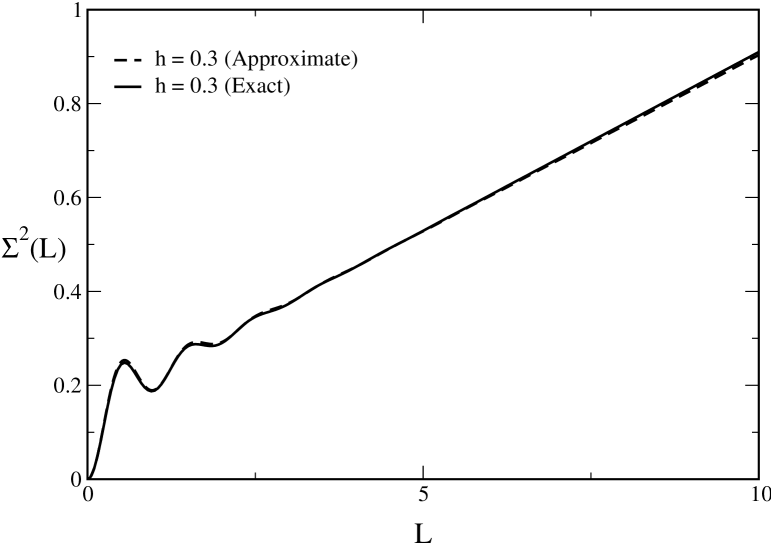
Figure 2: The number variance $\Sigma^{2}(L)$ versus $L$ for a value of $h=0.3$. The exact result (full curve) and the approximate result (dashed curve) nearly coincide.

The number variance of the eigenvalues near $x=0$ is obtained by integrating the two-point correlation function including the self-correlations

$$\Sigma^{2}(L)=\int_{0}^{L/\bar{\rho}(h)}dx\int_{0}^{L/\bar{\rho}(h)}dy\left[\delta(x-y)\langle\rho(x)\rangle+R_{2}(x,y)\right].$$ (74)

We study its asymptotic behavior in the limit $L\rightarrow\infty$. Starting from the expressions (58) and (66), $\Sigma^{2}(L)$ can be simplified by means of an orthogonality relation for Bessel functions. To leading order in $h$ we find

$$\Sigma^{2}(L) = \int_{0}^{L/\bar{\rho}(h)}xdx\int_{0}^{\infty}kdk\frac{J_{\nu}^{2}(kx)}{4\cosh^{2}\frac{\beta}{2}(k^{2}-4n\omega)}$$ (75)

$$= \frac{L}{\bar{\rho}2\pi\beta\bar{k}}=\frac{h}{4}L.$$

The same asymptotic result can be derived from the analytical result (73) (In this case the average spectral density does not depend on $h$ (see 62).). Such linear term, first proposed in [31], is believed to be characteristic for universal critical statistics [37] valid at the mobility edge and has been related to the multifractality of the wave functions [56, 57, 58, 59].

In Fig. 2 we compare the number variance derived from the approximate analytical result (73) and from the exact result (66). Clearly, even for a value of $h$ as large as 0.3 the two curve are barely distinguishable.

The asymptotic linear behavior of the number variance seems to be contradicted by the sum rule

$$\int_{-\infty}^{\infty}dy[\delta(x-y)\langle\rho(x)\rangle+R_{2}(x,y)]=0.$$ (76)

The resolution of this paradox [41, 60] is probably best illustrated by considering the Poisson ensemble for $n$ uncorrelated eigenvalues with average spacing $\bar{\rho}$. To satisfy the sum-rule we have that $R_{2}(x,y)=\bar{\rho}/n$ instead of zero for uncorrelated eigenvalues resulting in the number variance $\Sigma_{2}(L)=L-L^{2}/n$. We conclude that an asymptotic linear behavior is possible if the thermodynamic limit is taken before the limit $L\rightarrow\infty$.

To make contact with the partially quenched effective partition function, for which the number of subsequent eigenvalues around zero that are correlated according to the chGUE scales as $\sqrt{n}$ [4, 5, 6, 7], we have to scale $h$ as $h\to h/\sqrt{n}$. In this limit microscopic universality [1, 8, 9, 10, 11, 12] is recovered for the interpolating chiral unitary ensemble.

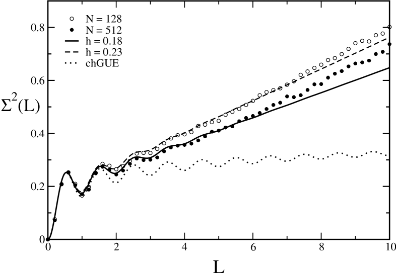
Figure 3: The number variance $\Sigma^{2}(L)$ versus $L$ for Dirac eigenvalues of instanton gauge field configurations (points) and our interpolating random matrix model. The total number of instantons and the parameter $h$ of our model are given in the label of the figure.

5 Comparison with Instanton Simulations

Spectral correlations have been studied in great detail for both lattice QCD simulations [4, 14, 15, 19, 17, 20, 21] and instanton-liquid simulations [5] (see [2] for a recent review). In lattice QCD they were studied by means of the disconnected scalar susceptibility [22], and complete agreement with partially quenched chiral perturbation theory was found. In particular, it was shown that the number of subsequent eigenvalues around zero described by chRMT scales as $F^{2}\sqrt{V}$. In instanton simulations a weaker volume dependence of the number of such eigenvalues was observed suggesting an approach to a critical point similar to a localization transition. Indeed the multifractality index of the fermionic wave functions was found to be nonzero. We thus compare the instanton data with the model in previous section at fixed value of the parameter $h$. Results for the number variance, $\Sigma^{2}(L)$ versus $L$ are shown in Fig. 3. The closed and open circles represent results [5] for the eigenvalues of the Dirac operator with field configurations given by an ensemble of instantons and an equal number of anti-instantons with a total density of 1 $fm^{4}$. The total number of (anti-)instantons is given in the label of the figure. In the same figure we show the result for the chGUE (dotted curve) and results for the model (66) for $h=0.18$ (full curve) and $h=0.23$ (dashed curve). We observe that both the slope and the range of agreement with the chGUE curve only shows a week volume dependence. Outside this domain the data show a linear $L$-dependence. Both features are nicely reproduced by the critical Random Matrix Model. The slightly positive curvature of the instanton data might be a remnant of the $L^{2}$ dependence predicted for the Altshuler-Shklovsky domain [31].

6 Conclusions

We have analyzed a chiral random matrix model that interpolates between the chGUE and the chiral Poisson ensemble. This model is a generalization of a model originally proposed by Moshe, Neuberger and Shapiro [40]. It has been mapped onto a gas of non-interacting fermions and was solved by means of statistical mechanics methods. To leading order in the deviation from the chGUE we have obtained compact analytical expressions for the microscopic spectral density and the two-point level correlation function. We have shown that this critical chiral random matrix model provides a good description of the level correlations of Dirac eigenvalues for gauge field configurations given by a liquid of instantons.

The number variance of the critical chiral random matrix model shows a linear $L$-dependence for a large $L$ (in units of the average level spacing) whereas it coincides with the chGUE result for small values of $L$. The characteristic feature is that the transition point between these two domains is stable in the thermodynamic limit. This situation is very different for a non-linear $\sigma$-model description of disordered systems where this transition point or the Thouless energy is determined by the competition between the mass term and the kinetic term. In that case one finds the scaling behavior $E_{c}\sim D/L^{2}_{s}$ with $D$ the diffusion constant and $L_{s}$ the linear size of the sample. The theoretical reason for a scale independent dimensionless conductance (i.e. the Thouless energy in units of the average level spacing) is that the localization length diverges at a critical value of the disorder. In the approach to this limit the diffusion constant has to become scale dependent. If $E_{c}$, in units of the average level spacing, becomes scale independent the diffusion constant has to be scale dependent leading to a multi-fractal scaling of the wave functions.

The weak volume dependence and the linear number variance observed in correlations of eigenvalues of the QCD Dirac operator with instanton liquid gauge field configurations suggests that we are dealing with a critical system close to a localization transition. Indeed the same numerical simulations suggest a small nonzero multifractality index of the wave-functions. On the other hand, the dimensionless conductance found in lattice QCD simulations scales according to our expectations from chiral perturbation theory. At this moment we do not have a good explanation for this discrepancy. It could simply be that the expected scaling behavior is only recovered for much large volumes in instanton simulations. Indeed, a very slow approach to the thermodynamic limit has been found for other quantities such a quenched chiral logarithms. Clearly, more work has to be done to resolve this issue.

Acknowledgements

This work was partially supported by the US DOE grant DE-FG-88ER40388. One of us (A.M.G.) was supported by “laCaixa Fellowship Program”. J.J.M.V. thanks the Institute for Nuclear Theory at the University of Washington for its hospitality and partial support during the completion of this work. Dominique Toublan is thanked for a critical reading of the manuscript.

References

- [1] E.V. Shuryak and J.J.M. Verbaarschot, Nucl. Phys. A560 (1993) 306.
- [2] J.J.M. Verbaarschot and T. Wettig, Ann. Rev. Nucl. Part. Sci. (2000), hep-ph/0003017.
- [3] J.J.M. Verbaarschot, Lectures given at APCTP - RCNP Joint International School on Physics of Hadrons and QCD, Osaka, Japan, 1998 and the 1998 YITP Workshop on QCD and Hadron Physics, Kyoto, Japan, 1998, hep-ph/9902394.
- [4] J.J.M. Verbaarschot, Phys. Lett. B368 (1996) 137.
- [5] J.C. Osborn and J.J.M. Verbaarschot, Phys. Rev. Lett. 81, 268 (1998); Nucl. Phys. B525 (1998) 738.
- [6] J.C. Osborn, D. Toublan and J.J.M. Verbaarschot, Nucl. Phys. B540 (1999) 317.
- [7] P.H. Damgaard, J.C. Osborn, D. Toublan and J.J.M. Verbaarschot, Nucl. Phys.B547 (1999)305.
- [8] E. Brézin, S. Hikami and A. Zee, Nucl. Phys. B464 (1996) 411.
- [9] G. Akemann, P.H. Damgaard, U. Magnea and S. Nishigaki, Nucl. Phys. B 487[FS] (1997) 721.
- [10] A.D. Jackson, M.K. Sener and J.J.M. Verbaarschot, Nucl. Phys. B479 (1996) 707.
- [11] T. Guhr and T. Wettig, Nucl. Phys. B506 (1997) 589.
- [12] A.D. Jackson, M.K. Sener and J.J.M. Verbaarschot, Nucl. Phys. B506 (1997) 612.
- [13] M.A. Halasz and J.J.M. Verbaarschot, Phys. Rev. Lett. 74 (1995) 3920; M.A. Halasz, T. Kalkreuter and J.J.M. Verbaarschot, Nucl. Phys. Proc. Suppl. 53 (1997) 266.
- [14] M.E. Berbenni-Bitsch, S. Meyer, A. Schäfer, J.J.M. Verbaarschot and T. Wettig, Phys. Rev. Lett. 80 (1998) 1146.
- [15] M.E. Berbenni-Bitsch, M. Gockeler, T. Guhr, A.D. Jackson, J.Z. Ma, S. Meyer, A. Schäfer, H.A. Weidenmüller, T. Wettig and T. Wilke, Phys. Lett. B438 (1998) 14.
- [16] M.E. Berbenni-Bitsch, M. Göckeler, T. Guhr, A.D. Jackson, J.-Z. Ma, S. Meyer, A. Schäfer, H.A. Weidenmüller, T. Wettig, and T. Wilke, Phys. Lett. B 438 (1998) 14.
- [17] P.H. Damgaard, U.M. Heller, and A. Krasnitz, Phys. Lett. B 445 (1999) 366.
- [18] M. Gockeler, H. Hehl, P.E.L. Rakow, A. Schafer and T. Wettig, Phys. Rev. D59 (1999) 094503.
- [19] R.G. Edwards, U.M. Heller, J. Kiskis, and R. Narayanan, Phys. Rev. Lett. 82 (1999) 4188.
- [20] B.A. Berg, H. Markum, and R. Pullirsch, Phys. Rev. D59 (1999) 097504.
- [21] F. Farchioni, I. Hip, and C.B. Lang, Phys. Lett.B471 (1999) 58;
- [22] M.E. Berbenni-Bitsch, M. Göckeler, H. Hehl, S. Meyer, P.E.L. Rakow, A. Schäfer, and T. Wettig, Phys. Lett. B466 (1999) 293; hep-lat/9908043.
- [23] R. Gade and F. Wegner, Nucl. Phys. B360 (1991) 213; R. Gade, Nucl. Phys. B398 (1993) 499.
- [24] A. Altland and B.D. Simons, Nucl. Phys. B562 (1999) 445.
- [25] K. Takahashi and S. Iida, hep-th/9903119.
- [26] T. Guhr, T. Wilke, and H.A. Weidenmüller, hep-th/9910107.
- [27] J. Gasser and H. Leutwyler, Phys. Lett. 188B(1987) 477; Nucl. Phys. B307 (1988) 763.
- [28] H. Leutwyler and A. Smilga, Phys. Rev. D46 (1992) 5607.
- [29] C. Bernard and M. Golterman, Phys. Rev. D46 (1992) 853; ; S. Sharpe, Phys. Rev. D46 (1992) 3146.
- [30] C. Bernard and M. Golterman, Phys. Rev.D49 (1994) 486; C. Bernard and M. Golterman, hep-lat/9311070; M.F.L. Golterman and K.C. Leung, hep-lat/9711033; M.F.L. Golterman, Acta Phys. Polon. B25 (1994).
- [31] B.L. Altshuler and B.I. Shklovskii, Zh. Eksp. Teor. Fiz. 91, 343 (1986); B.L. Altshuler, I.Kh. Zharekeshev, S.A. Kotochigova and B.I. Shklovskii, Zh. Eksp. Teor. Fiz. 94 (1988) 343.
- [32] T. Guhr, A. Müller-Groeling and H.A. Weidenmüller, Phys. Rep. 299 (1998) 189.
- [33] G. Montambaux, in Quantum Fluctuations, Les Houches, Session LXIII, E. Giacobino, S. Reynaud and J. Zinn-Justin, eds., Elsevier Science, 1995, cond-mat/9602071.
- [34] D. Braun and G. Montambaux, Phys. Rev. B52, (1995) 13903.
- [35] T. Banks and A. Casher, Nucl. Phys. B169 (1980) 103.
- [36] A. Aronov, V. Kravtsov and I. Lerner, Phys. Rev. Lett. 74, 1174 (1995).
- [37] B.I. Shklovskii, B. Shapiro and B.R. Sears, P. Lambrianides and H.B. Shore, Phys. Rev. B47 (1993) 11487.
- [38] A. Mirlin, Phys. Rep. (2000), cond-mat/9907136; M. Janssen, Phys. Rep. 295 (1998) 1.
- [39] I.Kh. Zharekshev and B. Kramer, Ann. Phys. (Leipzig) 7 (1998), 442.
- [40] M. Moshe, H. Neuberger and B. Shapiro, Phys. Rev. Lett. 73 (1994) 1497.
- [41] V. Kravtsov and K. Muttalib, Phys. Rev. Lett. 79, 1913(1997).
- [42] V.A. Kazakov and A.A. Migdal, Nucl. Phys. B397 (1993) 214.
- [43] T.H. Seligman, J.J.M. Verbaarschot and M.R. Zirnbauer, J. Phys. A: Math. Gen. 18 (1985) 2751.
- [44] A.D. Mirlin, Y.V. Fyodorov, F.M. Dittes, J. Quezada and T.H. Seligman, Phys. Rev. E 54 (1996) 3221.
- [45] K.A. Muttalib, Y. Chen, M.E.H. Ismail and V.N. Nicopoulos, Phys. Rev. Lett. 71 (1993) 471.
- [46] Y. Chen, M.E.H. Ismail and K.A. Muttalib, J. Phys. Cond. Mat. 4 (1992) L417; 5 (1993) 177.
- [47] S.M. Nishigaki, Phys.Rev. E58 (1998) R6915; Phys.Rev. E59 (1999) 2853.
- [48] F.A. Berezin and F.I. Karpelevich, Doklady Akad. Nauk SSSR 118 (1958) 9.
- [49] T. Guhr and T. Wettig, J. Math. Phys. 37 (1996) 6395.
- [50] A.D. Jackson, M.K. Şener and J.J.M. Verbaarschot, Phys. Lett. B 387 (1996) 355.
- [51] M. Caselle, A. D’Adda and S. Panzeri, Phys. Lett. B293 (1992) 161.
- [52] D. Boulatov and V.A. Kazakov, Int. J. Mod. Phys. A8 (1993) 809.
- [53] J. Verbaarschot and I. Zahed, Phys. Rev. Lett. 70, 3852 (1993).
- [54] J. Verbaarschot, Phys. Rev. Lett. 72 (1994) 2531; Phys. Lett. B329 (1994) 351.
- [55] E. Kanzieper, private communication.
- [56] B. Huckenstein and L. Schweitzer, Phys. Rev. Lett. 72 (1994) 713.
- [57] J. Chalker and V. Kravtsov and I. Lerner, JETP Lett. 64 (1996) 836.
- [58] J. Chalker, I. Lerner and R. Smith, Phys. Rev. Lett. 77 (1996) 554.
- [59] V.E. Kravtsov and A.M. Tsvelik, cond-mat/0002120.
- [60] V. Kravtsov, in Proceedings of Correlated Fermions and Transport in Mesoscopic Systems, Moriond Conference, Les Arcs, 1996, cond-mat/9603166.