Non-supersymmetric cousins of supersymmetric gauge theories:
quantum space of parameters and double scaling limits

Abstract

I point out that standard two dimensional, asymptotically free, non-linear sigma models, supplemented with terms giving a mass to the would-be Goldstone bosons, share many properties with four dimensional supersymmetric gauge theories, and are tractable even in the non-supersymmetric cases. The space of mass parameters gets quantum corrections analogous to what was found on the moduli space of the supersymmetric gauge theories. I focus on a simple purely bosonic example exhibiting many interesting phenomena: massless solitons and bound states, Argyres-Douglas-like CFTs and duality in the infrared, and rearrangement of the spectrum of stable states from weak to strong coupling. At the singularities on the space of parameters, the model can be described by a continuous theory of randomly branched polymers, which is defined beyond perturbation theory by taking an appropriate double scaling limit.

a Introduction and overview of the results

In recent years, notable successes have been achieved in understanding strongly coupled quantum field theories and string theories in various space-time dimensions, by combining old heuristic ideas with the power of supersymmetry. Perhaps most striking amongst these are the results on four dimensional, asymptotically free, gauge theories. In [1], Seiberg and Witten, and Seiberg, were able to compute the exact quantum corrections to the moduli space of vacua of various $N=1$ and $N=2$ gauge theories, using a subtle generalization of Montonen-Olive electric/magnetic duality [2] valid at low energy. In [3] a concrete proposal was made, in some particular supersymmetric examples, for the long-suspected string description of gauge theories [4], particularly when the number of colors is large. Unfortunately, these works rely heavily on very special mathematical properties of supersymmetric theories, and it has been impossible so far to assess their relevance to the non-supersymmetric world.

The purpose of this letter is to provide a framework where the relevance of supersymmetric models for non-supersymmetric gauge theories can be precisely studied. The idea is to consider a class of asymptotically free quantum field theories in two space-time dimensions which are distinguished by the fact that the low energy coupling can be changed by varying mass parameters, which thus play the rôle of Higgs expectation values. Versions of these theories with four supercharges show quantitative similarities with $N=2$ super Yang-Mills [5], and are thus the best possible toy models for the four dimensional supersymmetric gauge theories.

In this work, two main results are obtained. First, we will see that non-supersymmetric versions of the models discussed in [5] are tractable as well, and do continue to display qualitatively the same physics. The quantum corrections to the space of mass parameters $\cal M$ (which is the analogue of the moduli space of four dimensional gauge theories) can be computed. Convincing evidence is found that the physics unraveled in supersymmetric gauge theories can be relevant in genuinely non-supersymetric models as well. Second, we will show that one can take a double scaling limit, in the sense of the “old” matrix models [6], when approaching the singularities on the quantum space of mass parameters. This possibility was not anticipated on the gauge theory side, and, if correct in this context, could potentially be of great theoretical interest to understand the field theory/string theory duality in four dimensions.

Our claims will be exemplified in this letter by studying a simple purely bosonic theory displaying a rich physics akin to what was found in the four dimensional supersymmetric gauge theories. The model is a natural generalization of both the ${\rm O}(N)$ non-linear sigma model and the sine-Gordon model. The fields parametrize the $N-1$ dimensional sphere ${\rm S}^{N-1}$, and the lagrangian is the sum of the standard ${\rm O}(N)$ symmetric kinetic term and an additional interaction term which, for $N=2$, reduces to the sine-Gordon potential. Classically, this latter term gives a mass $\sim m$ to the would-be Goldstone bosons. Quantum mechanically, when $m$ is much larger that the dynamically generated “hadronic” mass scale $\Lambda$, the theory is weakly coupled and much of the physics can be read off from the lagrangian. On the contrary, when $m\sim\Lambda$, strong quantum corrections are expected. When $m=0$ we recover the standard ${\rm O}(N)$ non-linear sigma model, which has a mass gap and a spectrum made of a single particle in the vector representation of ${\rm O}(N)$ [7].

The quantum space of parameters ${\cal M}_{\rm q}$ can be worked out by using various techniques, including a large $N$ approximation. The submanifold of singularities $\cal H$, defined to be the locus in $\cal M$ where some of the degrees of freedom are massless, drastically changes when one goes from the classical to the quantum regime. Typically, either ${\cal H}_{\rm cl}$ locally splits into two, or does not change its shape, but in both cases the low energy physics is different in the classical and the quantum theory. Globally we obtain a hypersurface of singularities ${\cal H}_{\rm q}$ which delimits two regions on ${\cal M}_{\rm q}$, one at strong coupling and the other extending to weak coupling. On some regions of ${\cal H}_{\rm q}$, both a soliton, which is in our model a generalization of the sine-Gordon soliton, and a bound state of the elementary fields, become massless. The physics in the infrared is then governed by a non-trivial conformal field theory, either an Ising model or an ${\rm O}(2)$ symmetric Ashkin-Teller model. Kramers-Wannier duality exchanges the soliton and the bound state, and inside ${\cal H}_{\rm q}$ the notion of a topological charge is ambiguous. The dictionary with phenomena in four dimensional supersymmetric gauge theories is the following: our non-trivial CFTs are like Argyres-Douglas CFTs [8], the sine-Gordon soliton corresponds to a ’t Hooft-Polyakov monopole and Kramers-Wannier duality is mapped onto Montonen-Olive duality.

Another aspect of the model is that its $1/N$ expansion can be interpreted as a sum over topologies for randomly branched polymers. In particular, for some values of the parameters, the model has an ${\rm O}(N-1)$ symmetry and can be viewed as a $(N-1)$-vector model with an infinite number of interactions (bonds involving an arbitrary number of molecules in the branched polymers). One can approach the critical surface ${\cal H}_{\rm q}$ by taking a suitable double scaling limit, which on the one hand gives a description of the model in terms of extended objects (the polymers), and on the other hand defines non-perturbatively a continuous theory of polymers in a fully consistent context. In particular, the model overcomes notorious difficulties with double scaling limits in two dimensions [9].

b The model and its semi-classical properties

We will work with a space-time of euclidean signature and write the lagrangian of the model as

$$L={1\over 2}\sum_{i=1}^{N}\partial_{\mu}\phi_{i,0}\,\partial_{\mu}\phi_{i,0}+{\alpha\over 2}\,\biggl{(}\sum_{i=1}^{N}\phi_{i,0}^{2}-{1\over g_{0}^{2}}\biggr{)}+V_{\rm m}.$$ (1)

$\alpha$ is a Lagrange multiplier implementing the constraint that the target space is a sphere of radius $1/g_{0}^{2}$. Without the mass term $V_{\rm m}$, the theory is made UV finite by simple multiplicative renormalizations of the fields and coupling [10]. In the leading $1/N$ approximation, only the coupling constant renormalization is needed, and we will take the renormalized fields $\phi_{i}=\phi_{i,0}$, and coupling constant $g$ such that

$${1\over g^{2}}={1\over g_{0}^{2}}+{N\over 2\pi}\,\log{\mu\over\Lambda_{0}}={N\over 2\pi}\,\log{\mu\over\Lambda}\,\raise 2.0pt\hbox{,}$$ (2)

where $\Lambda_{0}$ is the UV cut-off, $\mu$ is a sliding scale, and $\Lambda$ is the dynamically generated mass scale of the theory. A mass term $V_{\rm m}$ is characterized by the canonical dimension of the mass parameters and the way they transform under ${\rm O}(N)$. For example, a magnetic field has canonical dimension 2 and transforms in the vector representation. Once these data are fixed, the explicit form of $V_{\rm m}$ is deduced from renormalization theory. In our model, the mass parameters will be taken to have canonical dimension 2 and to transform as a symmetric traceless rank two tensor $h_{ij}$ (they are like a tensor magnetic field). In general, $h_{ij}$ is multiplicatively renormalized; no renormalization is actually needed in the leading $1/N$ expansion. By diagonalizing $h_{ij}$ we can write

$$V_{\rm m}=-{1\over 2}\,\sum_{i=1}^{N}h_{i}\,\phi_{i}^{2}.$$ (3)

The trace part of $h_{ij}$ would correspond to a constant term in the lagrangian, and can thus be taken to be non zero without affecting the physics. We will use the $N-1$ independent dimensionless physical parameters $v_{i}=(h_{N}-h_{i})/\Lambda^{2}$ and $\cal M$ will be the $v$-space. Using the permutation symmetry amongst the $h_{i}$s, we will restrict ourselves to the region ${\cal M}^{+}$ of positive $v_{i}$s unless explicitly stated otherwise. The classical masses of the $N-1$ independent elementary fields $\phi_{i}$, $1\leq i\leq N-1$, are then $m_{i}=\Lambda\sqrt{v_{i}}$.

The model has always $N$ ${\mathbb{Z}}_{2(i)}$ symmetries $\phi_{i}\mapsto-\phi_{i}$, and can also have additional ${\rm O}(p)$ symmetries when $p$ of the $v_{i}$s coincide.

Singularities on ${\cal M}^{+}$ are found classically when some, say $p$, of the $v_{i}$s vanish. The low energy physics is then governed by a standard ${\rm O}(p+1)$ non linear sigma model, and the $p$ massless states are the $p$ classical Goldstone bosons for the breaking of ${\rm O}(p+1)$ down to ${\rm O}(p)$. ${\cal H}_{\rm cl}$ in ${\cal M}^{+}$ thus coincide with the hyperplanes $v_{i}=0$.

Quantum mechanically, in the weakly coupled region $v_{i}\gg 1$, we can use semiclassical techniques to investigate the spectrum of particles further. It can be shown that a bound state $\phi$-$\phi$ is associated with the operator $\phi_{N}^{2}=1/g_{0}^{2}-\sum_{i=1}^{N-1}\phi_{i}^{2}$. We will compute the mass of this state, for any $v_{i}$s, in the next section. One can also show that the model admits solitons connecting the two degenerate minima of the potential (3) at $\phi_{N}=\pm 1/g^{2}$. These two minima are related by the spontaneously broken ${\mathbb{Z}}_{2(N)}$ symmetry. All the solitonic (time independent, finite energy) solutions can be explicitly found [11]. In the simple ${\rm O}(N-1)$ symmetric case where $v_{1}=\cdots=v_{N-1}=v\gg 1$, they correspond to trajectories joining the two poles at $\phi_{N}=\pm 1/g^{2}$ along a meridian of the target space sphere. They are standard sine-Gordon solitons of masses $M_{\rm cl}=2\Lambda\sqrt{v}/g^{2}$. The semi-classical quantization shows that the solitons are particles filling multiplets of ${\rm O}(N-1)$ corresponding to the completely symmetric traceless tensor representations. The rank $J$ tensor has a mass $M_{J}=M_{\rm cl}+J(J+N-3)v\Lambda^{2}/(2M_{\rm cl})$.

c The large N approximation

A useful technique to study our model is to use a large $N$ approximation (for a recent review, see [12]), where $N$ is sent to infinity while the scale $\Lambda$ is held fixed [4]. The large $N$ expansion is nothing but a standard loop expansion for a non-local effective action $S_{\rm eff}$ obtained by integrating exactly a large number of elementary fields $\phi_{i}$ from (1). For our purposes, it will be useful to keep explicitly the order parameter $\phi_{N}=\sqrt{N}\varphi$ for ${\mathbb{Z}}_{2(N)}$ in the action. The effective action for large $N$ is then

$${S_{\rm eff}\over N}=\int\!d^{2}x\,\biggl{\{}{1\over 2}\,\partial_{\mu}\varphi\,\partial_{\mu}\varphi+{\alpha-h_{N}\over 2}\,\varphi^{2}-{\alpha\over 2Ng^{2}}\biggr{\}}+{1\over N}\sum_{i=1}^{N-1}s\bigl{[}\alpha-h_{i}\bigr{]},$$ (4)

where $s[f]=(1/2)\mathop{\rm tr}\nolimits\ln(-\partial^{2}+f)-\ln(\Lambda_{0}/\mu)\int d^{2}xf/(4\pi)$ can be expanded in terms of ordinary Feynman diagrams.

It is useful to compute, in this framework, the masses of the particles we found previously in a semi-classical approximation. At leading order, this is done by looking at poles in the two-point functions derived from (4). In the ${\rm O}(N-1)$ symmetric case $v_{1}=\cdots=v_{N-1}=v$, and for $v>1$, the $N-1$ elementary fields $\phi_{i}$ have a mass $m_{\phi}=\Lambda\sqrt{v}$, and the mass $m_{\rm b}$ of the $\phi$-$\phi$ bound state (the field $\varphi$) is a solution of

$$\sqrt{4\Lambda^{2}v/m_{\rm b}^{2}-1}\,\ln v=2\arctan\biggl{(}1\!\Bigm{/}\!\sqrt{4\Lambda^{2}v/m_{\rm b}^{2}-1}\biggr{)}.$$ (5)

$m_{\rm b}$ is a monotonic function of $v$, decreasing from $m_{\rm b}\simeq 2m_{\phi}\bigl{(}1-(Ng^{2})^{2}/32\bigr{)}$ for $v\gg 1$ to $m_{\rm b}=0$ for $v=1$. The mass of the ${\rm O}(N-1)$ singlet soliton also goes to zero as $v$ goes to one because the two degenerate minima of the effective potential derived from $S_{\rm eff}$ merge at $v=1$. More generally, the $\phi$-$\phi$ bound state and the lightest solitonic state will become massless together on the critical hypersurface $\prod_{i=1}^{N-1}v_{i}=1$. Near this hyperboloid, the $1/N$ expansion has IR divergencies and is no longer reliable. These divergencies are due to the fact that we are near a critical point below the critical dimension. To describe the physics near the critical surface, we must go beyond the $1/N$ approximation and sum the most relevant (i.e. the most IR divergent) contributions. This also automatically resolves the difficulties associated with massless propagators in two dimensions. One can show that the low energy effective lagrangian on the critical surface is, in the large $N$ limit,

$$L_{\rm eff}={1\over 2}\,\partial_{\mu}\phi_{N}\,\partial_{\mu}\phi_{N}+{\pi\Lambda^{2}\over\sum_{i=1}^{N-1}1/v_{i}}\,\,\phi_{N}^{4},$$ (6)

where the interaction, which is proportional to $1/N$, must be treated exactly, since the IR divergencies compensate for the $1/N$ factors. We thus obtain the Landau-Ginzburg description of an Ising critical point. The field $\phi_{N}$ is the order operator and the massless soliton corresponds to the disorder operator; they are exchanged by Kramers-Wannier duality. Displacements on the critical surface are associated here with irrelevant operators in the IR.

It is important to note that the $1/N$ corrections to the equation of the critical surface itself only suffer from mild logarithmic IR divergencies that can be handled [11]. The existence and form of this surface can thus be reliably studied in a $1/N$ expansion. We will see that the critical surface actually intersects with the hyperplanes $v_{i}=0$, and thus join with the other sheet of the surface existing for $v_{i}<0$. The relevant physics is discussed in the following section.

d The quantum space of parameters

There are regions in the space of parameters where it is easy to see that the classical and quantum hypersurfaces of singularities coincide. When one of the $v$s is zero, say $v_{1}=0$, and all the other $v$s are large, the low energy theory is an ${\rm O}(2)$ sigma model of small effective coupling $g_{\rm eff}$. Both classically and quantum mechanically, this is a massless theory, and thus ${\cal H}_{\rm cl}={\cal H}_{\rm q}=\bigl{\{}v_{1}=0\bigr{\}}$ in this region. However, the physics are not the same: the classical theory of a free massless boson is replaced in the quantum case by the non-trivial CFT of a boson compactified on a circle of radius $R$ with $R^{2}=4\pi/g_{\rm eff}^{2}=\ln(\prod_{i=2}^{N-1}v_{i})$. If $p$ of the $v_{i}$s, $i\geq 2$, decrease, while we stay on the hyperplane $v_{1}=0$, the low energy theory will tend to become an ${\rm O}(p+2)$ non linear sigma model and thus develop a mass gap. In the large $N$ limit, it can be shown that this transition takes place on a surface ${\mathfrak{h}}_{{\rm q},1}$ whose equation is $\prod_{i=2}^{N-1}v_{i}=1$, $v_{1}=0$, and that the low energy theory on ${\mathfrak{h}}_{{\rm q},1}$ is an ${\rm O}(2)$ symmetric Ashkin-Teller model with Landau-Ginzburg potential

$$V_{\rm eff}={\pi\Lambda^{2}\over\sum_{i=2}^{N-1}1/v_{i}}\,\,\Bigl{(}\phi_{1}^{2}+\phi_{N}^{2}\Bigr{)}^{2}.$$ (7)

This model is indeed equivalent to a compactified boson for the particular radius $R=R_{\rm KT}=2\sqrt{2}$, and the transition through ${\mathfrak{h}}_{{\rm q},1}$ is nothing but a Kosterlitz-Thouless phase transition. A local analysis shows that ${\cal H}_{\rm q}$ joins the hyperplane $v_{1}=0$ orthogonally along ${\mathfrak{h}}_{{\rm q},1}$, and that going from $v_{1}=0$ to $v_{1}>0$ on ${\cal H}_{\rm q}$ is equivalent to turning on a relevant operator which decouples one of the two Ising spins in the Ashkin-Teller model. The other spin would decouple in the $v_{1}<0$ region. We see that the Ashkin-Teller model on ${\mathfrak{h}}_{{\rm q},1}$ is made of the coupling of the two Ising models (one for $v_{1}>0$, the other for $v_{1}<0$) found in the preceding section.

It is possible to find a simple equation for ${\cal H}_{\rm q}$ valid for all values of the $v_{i}$s, positive or negative, in the large $N$ limit:

$${\cal H}_{\rm q}:\quad\sum_{i=1}^{N}\prod_{j\neq i}(r-h_{j})=\Lambda^{2(N-1)},$$ (8)

where $r$ is the largest real root of the polynomial $\prod_{i=1}^{N}(x-h_{i})-\tilde{\Lambda}^{2N}$. $\tilde{\Lambda}^{2N}$ can in principle be determined in terms of $\Lambda$ by a non-perturbative calculation. The fact that the Kosterlitz-Thouless transition occurs at a strictly positive radius $R_{\rm KT}$ implies $\tilde{\Lambda}<\Lambda$. The shape of ${\cal H}_{\rm q}$ is likely to be qualitatively reproduced by (8) even for small values of $N$, and we have used it to draw Fig. 1, which gives a global picture of the quantum space of parameters of our model in the case $N=4$.

e The double scaling limits

On the critical surface ${\cal H}_{\rm q}$, the sum of Feynman diagrams of a given topology (i.e. contributing at a fixed order in $1/N$) diverges. It is then natural to ask whether it is possible to approach ${\cal H}_{\rm q}$ and take the limit $N\rightarrow\infty$ in a correlated way in order to obtain a finite answer taking into account diagrams of all topologies. This is the idea of the double scaling limit [6], and for vector models the result can be interpreted as giving the partition function of a continuous theory of randomly branched polymers [13].

Let us consider for example the case of the ${\rm O}(N-1)$ symmetric theory $v_{1}=\cdots=v_{N-1}=v$. Near the critical point $v=1$, the effective theory is just given by (6) with the relevant perturbation $(1/2)\Lambda^{2}(1-v)\,\Phi_{N}^{2}$. The idea (used in [12]) is then to eliminate the explicit $N$ dependence in the interaction term by using a rescaled space-time variable $y=x/\sqrt{N}$,

$$S_{\rm eff}=\int\!d^{2}y\,\biggl{\{}{1\over 2}\,\partial_{\mu}^{y}\phi_{N}\,\partial_{\mu}^{y}\phi_{N}+{1\over 2}\Lambda^{2}N(1-v)\,\phi_{N}^{2}+\pi\Lambda^{2}\,\phi_{N}^{4}\biggr{\}}.$$ (9)

A consistent double scaling limit can be defined to be $N\rightarrow\infty$, $v\rightarrow 1$, with $N(v-1)-3\ln N$ kept fixed. The logarithmic correction to the naive scaling comes from the fact that the large $N$ limit is also a large UV cutoff limit in the $y$ variable, and (9) needs to be renormalized, which is done by a simple normal ordering. A similar non-trivial double scaling limit can be defined near the Ashkin-Teller point. For example, for $N\rightarrow\infty$, $v_{1}\rightarrow 0$, $v_{2}=\cdots=v_{N-1}=v\rightarrow 1$, the combinations that must be kept fixed are $N(v-1)-4\ln N$ and $N(v-v_{1}-1)-4\ln N$. Note that our theory in these limits is free of the inconsistencies found in the standard vector models in a similar context [9], as can be shown from a straightforward calculation of the 1PI effective action.

f Other models

It is possible to study other mass terms or/and other target spaces along the lines of the present work. It could also be interesting to perform lattice calculations for this class of models. For example, a mass term $m_{ij}=m_{ji}$ of canonical dimension one allows to obtain higher critical points. The quantum space of parameters of a ${\mathbb{C}}{\rm P}^{N}$ model with mass terms, which has instantons, a $\theta$ angle, and exhibit confinement at strong coupling, is also likely to display a rich structure. Finally, it is natural to consider supersymmetric versions of our models. It turns out that the massive version of the supersymmetric ${\mathbb{C}}{\rm P}^{N}$ model shows quantitative similarities with $N=2$ super Yang-Mills [5]. A discussion of these models along with details on the present work will be published elsewhere [11, 14].

I would like to thank Princeton University for offering me matchless working conditions.

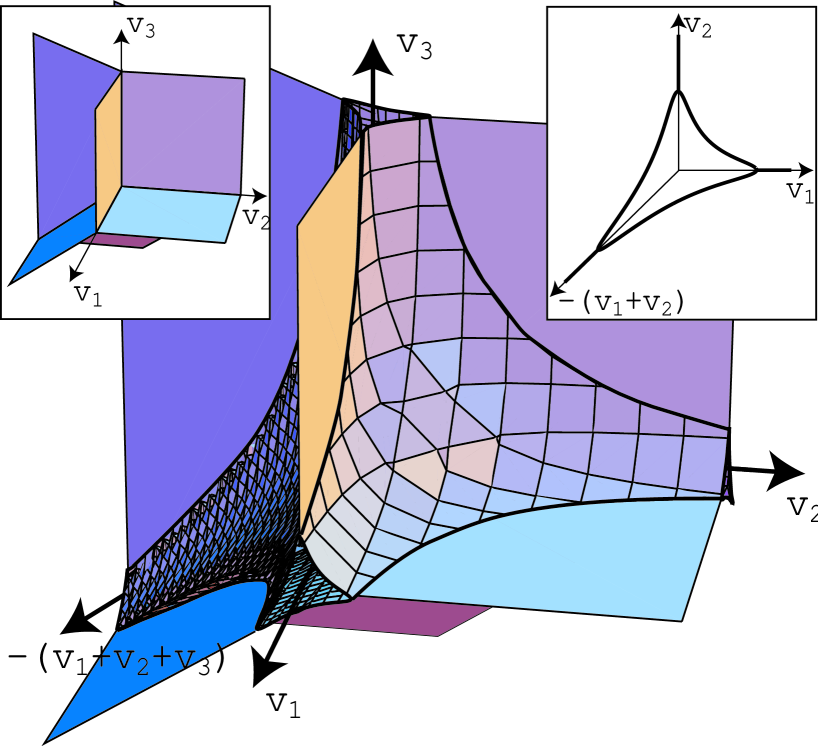
FIG. 1.: The classical (left inset) and quantum hypersurfaces of singularities ${\cal H}_{\rm cl}$ and ${\cal H}_{\rm q}$ in the case $N=4$. We chose $\tilde{\Lambda}/\Lambda=2/3$. Along the four tubes extending towards infinity, one of the fields is very massive and can be integrated out. A section of any of the tubes thus gives the curve of singularities for $N=3$, which is also represented (right inset). The CFTs on ${\cal H}_{\rm q}$ can be either an Ising critical point, an Ashkin-Teller critical point, or a compactified boson of any radius $R\geq R_{\rm KT}=2\sqrt{2}$.

REFERENCES

-
[1]
N. Seiberg and E. Witten, Nucl. Phys. B 426 (1994) 19;
430 (1994) 485(E); 431 (1994) 484,
N. Seiberg, Phys. Rev. D 49 (1994) 6857; Nucl. Phys. B 435 (1995) 129. - [2] C. Montonen and D. Olive, Phys. Lett. B 72 (1977) 117.
-
[3]
J. Maldacena, Adv. Theor. Math. Phys. 2 (1998) 231,
S.S. Gubser, I.R. Klebanov, and A.M. Polyakov, Phys. Lett. B 428 (1998) 105,
E. Witten, Adv. Theor. Math. Phys. 2 (1998) 253. - [4] G. ’t Hooft, Nucl. Phys. B 72 (1974) 461.
-
[5]
A. Hanany and K. Hori, Nucl. Phys. B 513 (1998) 119,
N. Dorey, JHEP 11 (1998) 005,
N. Dorey, T.J. Hollowood, and D. Tong, JHEP 5 (1999) 006,
F. Ferrari, to appear. -
[6]
É. Brézin and V.A. Kazakov, Phys. Lett. B 236 (1990)
144,
M.R. Douglas and S. Shenker, Nucl. Phys. B 355 (1990) 635,
D.J. Gross and A.A. Migdal, Phys. Rev. Lett. 64 (1990) 127. -
[7]
A.M. Polyakov, Phys. Lett. B 59 (1975) 79,
A.B. Zamolodchikov and Al. B. Zamolodchikov, Annals Phys. 120 (1979) 253. - [8] P.C. Argyres and M.R. Douglas, Nucl. Phys. B 448 (1995) 93.
- [9] P. Di Vecchia and M. Moshe, Phys. Lett. B 300 (1993) 49.
- [10] É. Brézin, J.C. Le Guillou, and J. Zinn-Justin, Phys. Rev. D 14 (1976) 2615.
- [11] F. Ferrari, A model for gauge theories with Higgs fields, PUPT-1962, LPTENS-00/28.
- [12] J. Zinn-Justin, lectures at the 11th Taiwan Spring School on Particles and Fields (1997), hep-th/9810198.
-
[13]
J. Ambjørn, B. Durhuus, and T. Jónsson, Phys. Lett. B 244 (1990) 403,
S. Nishigaki and T. Yoneya, Nucl. Phys. B 348 (1991) 787,
P. Di Vecchia, M. Kato, and N. Ohta, Nucl. Phys. B 357 (1991) 495. - [14] F. Ferrari, The supersymmetric non-linear sigma model with mass terms, to appear.