The String Dual of a Confining Four-Dimensional Gauge Theory

Abstract

We study ${\cal N}=1$ gauge theories obtained by adding finite mass terms to ${\cal N}=4$ Yang-Mills theory. The Maldacena dual is nonsingular: in each of the many vacua, there is an extended brane source, arising from Myers’ dielectric effect. The source consists of one or more $(p,q)$ 5-branes. In particular, the confining vacuum contains an NS5-brane; the confining flux tube is a fundamental string bound to the 5-brane. The system admits a simple quantitative description as a perturbation of a state on the ${\cal N}=4$ Coulomb branch. Various nonperturbative phenomena, including flux tubes, baryon vertices, domain walls, condensates and instantons, have new, quantitatively precise, dual descriptions. We also briefly consider two QCD-like theories. Our method extends to the nonsupersymmetric case. As expected, the ${\cal N}=4$ matter cannot be decoupled within the supergravity regime.

I Introduction

The proposal of ’t Hooft [1], that large-$N$ non-abelian gauge theory can be recast as a string theory, has taken an interesting turn with the work of Maldacena [2]. The principal Maldacena duality applies not to confining theories but to conformal ${\cal N}=4$ gauge theories, which are dual to IIB string theory on $AdS_{5}\times S^{5}$. Starting with this duality one can perturb by the addition of mass terms preserving a smaller supersymmetry, or none at all, and in this way obtain a confining gauge theory. The problem is that the perturbation of the dual string theory appears to produce a spacetime with a naked singularity [3]. As a consequence, even basic quantities such a condensates are incalculable.

In this paper we show that the situation is actually much better. There is no naked singularity, but rather an expanded brane source, and all physical quantities are calculable. We believe that this is the first example of a dual supergravity description of a four-dimensional confining gauge theory. It is also gives new insight into the resolution of naked singularities in string theory.

We focus on perturbations that preserve ${\cal N}=1$ supersymmetry, though in fact our solutions are stable under the addition of small additional masses that break the supersymmetry completely. The ${\cal N}=4$ vector multiplet contains an ${\cal N}=1$ vector multiplet and three ${\cal N}=1$ chiral multiplets. We will add finite ${\cal N}=1$ supersymmetry-preserving masses to the three chiral multiplets. For brevity we will refer to this theory as ‘${\cal N}=1^{*}$’. This theory has been studied by many authors [4, 5, 6, 7, 8]. It is known to have a rich phase structure [4, 5, 9], which includes confining phases that are in the same universality class as those of pure ${\cal N}=1$ Yang-Mills theory. We will show that the rich structure of this theory is reflected in supergravity in remarkable ways.

To study pure ${\cal N}=0$ or ${\cal N}=1$ Yang-Mills theories would require working at small ’t Hooft coupling and taking the masses of the extra multiplets to infinity. This is not tractable without an understanding of classical string theory in Ramond-Ramond backgrounds at large curvature. At large ’t Hooft coupling, where supergravity is valid, the masses of the extra multiplets must be kept finite. However, we emphasize these multiplets are four-dimensional and the ultraviolet theory is conformal. An alternative approach to obtaining a string dual of confining theories is via high-temperature five-dimensional supersymmetric field theories [10, 11, 12, 13], whose low-energy limit is four-dimensional strongly-coupled non-supersymmetric Yang-Mills theory. The dual spacetime is non-singular, and the infrared cutoff provided by the temperature does indeed lead to confinement of electric flux tubes. In this case, however, there is a full set of massive five-dimensional states that do not decouple.

Our work was motivated by the observation of Myers [14], that D-branes in a transverse Ramond-Ramond (RR) potential can develop a multipole moment under fields that normally couple to a higher-dimensional brane. This ‘dielectric’ property is analogous to the induced dipole moment of a neutral atom in an electric field. For example, a collection of $N$ D0-branes in an electric RR 4-form flux develops a dipole moment under the corresponding 3-form potential. One can think of them as blowing up into a spherical D2-brane, and in a strong field the latter is the effective description. This happens because the D0-brane coordinates become noncommutative. The original D0-brane charge $N$, which of course is conserved in this process, shows up as a nonzero world-volume field strength on the D2-branes. Even earlier, Kabat and Taylor [15] had observed that $N$ D0-branes with noncommuting position matrices could be used to build a spherical D2-brane in matrix theory, generalizing the flat membranes of matrix theory [16]. For finite $N$ the sphere is ‘fuzzy’; or better, perhaps, it is somewhat granular. The equations describing this sphere bear a marked similarity to those which appear in the ${\cal N}=1^{*}$ theory, which were first analyzed in [4].

It is then natural to guess that Myers’ mechanism is at work in this theory. The mass perturbation corresponds to a magnetic RR 3-form flux, which is dual to an electric RR 7-form flux. The latter couples to the D3-brane in the same fashion as the electric 4-form flux does to the D0-brane, and so the D3-branes polarize into D5-branes with world-volume ${\bf R}^{4}\times S^{2}$. One difference is that Myers considers D-branes in flat spacetime ($gN$ small), whereas for the gauge/gravity duality the background is $AdS_{5}\times S^{5}$. In Myers’ case a small field produced a small D2-sphere, but in the conformal field theory there is no invariant notion of a small mass perturbation, and on the supergravity side there is no such thing as a small transverse two-sphere. Rather, the D5-spheres, which are dynamically (though not topologically) stable, wrap an equator of the $S^{5}$. We will show that there exist supergravity solutions in which the only ‘singularity’ is that due to the D5-brane source on the $S^{5}$.

However, this is far from the whole story. First, the classical ${\cal N}=1^{*}$ theory has many isolated vacua [4]. For each partition of $N$ into integers $n_{i}$, there must be a separate solution involving multiple D5-branes with D3-branes charges $n_{i}$, each wrapped on an equator of $S^{5}$ but at different $AdS$ radii $r_{i}$ proportional to $n_{i}$. We will study these vacua, and their properties, in our discussion below. Second, the quantum theory has even more vacua, which are permuted under the $SL(2,{\bf Z})$ duality the field theory inherits from ${\cal N}=4$[5]. In particular, the transformation $\tau\to-{1\over\tau}$, which takes the maximally Higgsed vacuum into the confining vacuum, will replace the D5-brane sphere with an NS5-brane sphere: this is the effective string description of the confining vacuum. The confining flux tubes are bound states of a fundamental string to the NS5-brane, or equivalently, instantons of the 5-brane world-volume noncommutative gauge theory. Meanwhile, the leading nonperturbative condensate corresponds to the three-form field generated by the NS5-brane’s magnetic dipole moment.

Our removal of the singularity resembles phenomena that occur on the Coulomb branch [17, 18, 19, 20] and with the repulson singularity that arises in ${\cal N}=2$ supergravity duals [21]. There are certainly connections which need to be developed further, but the detailed mechanism is different. In particular, the appearance of NS-branes is new. Our result also gives insight into perturbations of the Randall-Sundrum compactification [23], and into recent proposals for the solution to the cosmological constant problem [24].

We begin in section II with a review of the classical and quantum field theory vacua, and a discussion of the corresponding brane configurations. In fact, there are more brane configurations than vacua, but later we will argue that only one configuration is applicable for any given value of the parameters. In section III we review perturbations of the $AdS$/CFT duality, with attention to the issue of the naked singularity. We show that there is a small parameter: the system can be regarded as a perturbation of one that has only D3-brane charges. This enables us to obtain a quantitative description even for the rather asymmetric and nonlinear supergravity configuration that results from the expansion of the branes. In section IV we study a simplified calculation, in which $n\ll N$ probe D3-branes are introduced into a fixed background. We find that their potential has minima where they form a D5-brane or NS5-brane, or more generally one or more $(c,d)$ 5-branes, wrapped on an equator of the $S^{5}$. In section V we consider the case that all $N$ D3-branes expand into 5-branes. Although this substantially deforms the geometry, serendipitous cancellations allow us to find the effective potential in a simple form: it is the same as in the probe case. We discuss the stability of the solution, arguing that it survives even when supersymmetry is broken completely. In section VI we use the dual description to discuss the physics of the gauge theory, including flux tubes and confinement, baryons, domain walls, condensates, instantons, and glueballs. In section VII we briefly discuss extensions, including the ${\cal N}=0$ case and orbifolds, and in section VIII we discuss implications and future directions.

II ${\cal N}=1^{*}$ Ground States

A Field Theory Background

In the language of four-dimensional ${\cal N}=1$ supersymmetry, the ${\cal N}=4$ theory consists of a vector multiplet $V$ and three chiral multiplets $\Phi_{i}$, $i=1,2,3$, all in the adjoint representation of the gauge group. In addition to the usual gauge-invariant kinetic terms for these fields, the theory has additional interactions summarized in the superpotential

$$W=\frac{2\sqrt{2}}{g_{\rm YM}^{2}}{\rm tr}([\Phi_{1},\Phi_{2}]\Phi_{3})\ .$$ (1)

The theory has an $SO(6)$ $R$-symmetry which is partially hidden by the ${\cal N}=1$ notation; only the $U(1)$ $R$-symmetry of the ${\cal N}=1$ supersymmetry and the $SU(3)$ that rotates the $\Phi_{i}$ are visible. However, if we write the lowest component of $\Phi_{i}$ as

$$\phi_{i}=\frac{A_{i+3}+iA_{i+6}}{\sqrt{2}}$$ (2)

(the reason for this notation will become evident later), then the potential energy for the scalar fields $A_{m}$, $m=4,\dots,9$, is explicitly $SO(6)$ invariant:

$$V(A_{m})\propto\sum_{m,n=4}^{9}{\rm tr}\left([A_{m},A_{n}][A_{m},A_{n}]\right)\ .$$ (3)

The theory is conformally invariant, and consists of a continuous set of theories indexed by a marginal coupling $\tau={\theta\over 2\pi}+i{4\pi\over g_{\rm YM}^{2}}$, where $\theta$ and $g_{\rm YM}$ are the theta angle and gauge coupling of the theory.

We can partially break the supersymmetry by adding arbitrary terms to the superpotential. Consider the addition of mass terms

$$\Delta W=\frac{1}{g_{\rm YM}^{2}}(m_{1}\,{\rm tr}\,\Phi_{1}^{2}+m_{2}\,{\rm tr}\,\Phi_{2}^{2}+m_{3}\,{\rm tr}\,\Phi_{3}^{2})\ .$$ (4)

If $m_{1}=m_{2}$ and $m_{3}=0$ the theory has ${\cal N}=2$ supersymmetry; otherwise it has ${\cal N}=1$. If $m_{1}=m_{2}=0$ and $m_{3}\neq 0$ then the theory flows to a conformal fixed point with a smooth moduli space and $SL(2,{\bf Z})$ duality [25, 26, 19, 27]. With two nonzero masses, the theory has a moduli space containing special subspaces where charged particles are massless and the Kähler metric is singular. However, in ${\cal N}=1^{*}$, where all three masses are non-zero, there is no moduli space; the theory has a number of isolated vacua. In the limit

$$\tau\to i\infty\ ,\quad m_{i}\to\infty\ ,\quad\Lambda^{3}=m_{1}m_{2}m_{3}e^{2\pi i\tau/N}\ {\rm fixed}$$ (5)

the theory becomes pure ${\cal N}=1$ Yang-Mills theory. For gauge group $SU(N)$ the pure ${\cal N}=1$ theory has $N$ vacua related by a spontaneously broken discrete $R$-symmetry. Note that this $R$-symmetry is not present in ${\cal N}=1^{*}$; it is an accidental symmetry present only in the limit Eq. (5).

The classical vacua were described by Vafa and Witten [4]. Assuming all masses are nonzero, we may rescale the fields $\Phi_{i}$ so as to make all the masses equal; having computed the vacua in this case one may undo this rescaling. In this case the $F$-term equations for a supersymmetric vacuum read

$$[\Phi_{i},\Phi_{j}]=-\frac{m}{\sqrt{2}}\epsilon_{ijk}\Phi_{k}\ .$$ (6)

Consider the case of $SU(N)$. Recalling that the $\Phi_{i}$ are $N\times N$ traceless matrices, it is evident that the solutions to these equations are given by $N$-dimensional, generally reducible, representations of the Lie algebra $SU(2)$. The irreducible spin $(N-1)/2$ representation is one solution; $N$ copies of the trivial representation give another ($\Phi_{i}=0$). Since for every positive integer $d$ there is one irreducible $SU(2)$ representation of dimension $d$, each vacuum corresponds to a partition of $N$ into positive integers:

$$\{k_{d}\in{\bf Z}\geq 0\}\ {\rm such\ that\ }\sum_{d=1}^{N}\ dk_{d}=N\ ,$$ (7)

where $k_{d}$ is the number of times the dimension $d$ representation appears. The number of classical vacua of the theory is given by the number of such partitions.

Generally, for a given partition, the unbroken gauge group is $\left[\otimes_{d}U(k_{d})\right]/U(1)$. For example, if $k_{d}=1$ and $k_{N-d}=1$, then the $\Phi_{i}$ are block diagonal with blocks of dimension $d$ and ${N-d}$; the diagonal traceless matrix which is ${\bf 1}$ in each block generates an unbroken $U(1)$ gauge symmetry. Clearly we obtain $U(1)^{k-1}$ if there are $k$ such blocks. However, if $k_{d}=2$, then the two blocks of size $d$ can be rotated into each other by additional generators, giving altogether an $SU(2)$ instead of a $U(1)$. More generally we obtain $SU(k_{d})$. Among these vacua there is a unique one which we will call the ‘Higgs’ vacuum, in which the $SU(N)$ gauge group is completely broken. This is the only ‘massive vacuum’ (meaning that it has a mass gap) at the classical level. For each divisor $d<N$ of $N$ we may take $k_{d}=N/d$ with all others zero, giving a vacuum with a simple unbroken gauge group $SU(N/d)$. All other vacua have one or more $U(1)$ factors; these are ‘Coulomb vacua.’

Quantum mechanically, the story is even richer. Donagi and Witten [5] found an integrable system which permitted them to write the holomorphic curve and Seiberg-Witten form describing the quantum mechanical moduli space of the ${\cal N}=2$ theory with $m_{1}=m_{2}$ and $m_{3}=0$. They considered the effect of breaking the supersymmetry to ${\cal N}=1$ through nonzero $m_{3}\ll m_{1},m_{2}$, and showed that the theory has a number of remarkable properties. Each classical vacuum which has unbroken gauge symmetry $SU(k)$ splits into $k$ vacua, all of which have a mass gap. (Coulomb vacua with non-abelian group factors split as well, although a complete accounting of these vacua was not given in [5]; since the photons remain massless, such vacua do not have mass gaps.) The vacuum with $SU(N)$ unbroken ($k_{1}=N$, $\Phi_{i}=0$) splits into $N$ massive vacua, exactly the number which would be needed in the ${\cal N}=1$ Yang-Mills theory obtained in the limit Eq. (5). The massive quantum vacua are those without $U(1)$ factors, and as noted above are associated with the divisors of $N$. Their total number is obviously given by the sum of the divisors of $N$; it therefore depends in an interesting way, one which does not have a large-$N$ limit, on the prime factors of $N$. The number of Coulomb vacua is exponential in $\sqrt{N}$.

Donagi and Witten showed the massive vacua were in a beautiful one-to-one correspondence with the phases of gauge theories classified by ’t Hooft. Let us review this classification [28]. $SU(N)$ gauge theories with only adjoint matter can be probed by sources which carry electric charges in the ${\bf Z}_{N}$ center of $SU(N)$ and magnetic charges in the ${\bf Z}_{N}=\pi_{1}[SU(N)/{\bf Z}_{N}]$ which characterizes possible Dirac strings. We may think of these charges as lying in an $N\times N$ lattice, a ${\bf Z}_{N}\times{\bf Z}_{N}$ group $L$. ’t Hooft showed that the possible massive phases of $SU(N)$ gauge theories are associated to the dimension-$N$ subgroups $P$ of $L$. In each phase, the charges corresponding to the $N$ elements of $P$ are screened, and all others are confined; the flux tubes which do the confining are represented by the elements of $L/P$. For example, if the ordinary Higgs mechanism creates a mass gap, all sources with magnetic charge are confined; the only unconfined elements of $L$ are the $(m,0)$, $m=0,\dots,N-1$. Thus $P$ is generated by the single element $(1,0)$. Every magnetic flux tube carries a ${\bf Z}_{N}$ charge $n=0,\dots,N-1$ and confines the sources with charge $(m,n)$ for any $m$. In an ordinary confining vacuum, the roles of $m$ and $n$ are reversed, but otherwise the story is the same. Vacua with oblique confinement are given by groups $P$ generated by $(m,1)$, where $m=0,\dots,N-1$.

More generally, however, the vacua are more complex. As mentioned earlier, each classical vacuum with unbroken $SU(k)$ symmetry splits into $k$ vacua. These vacua correspond to subgroups $P$ generated by $(k,0)$ and $(s,d)$, where $dk=N$ and $s=0,1,\dots,k-1$. This map of vacua to subgroups is one-to-one and onto. Note the Higgs vacuum is the case $d=N$, while the $N$ vacua which survive in the pure ${\cal N}=1$ Yang-Mills theory are the cases $d=1$ for $s=0,1,\dots,N-1$, with $s=0$ being the confining vacuum.

The action of $SL(2,{\bf Z})$ on the massive vacua is then straightforward [5]. The $T$ transformation $\tau\to\tau+1$ shifts each element $(m,n)$ of the group $L$ to $(m+n\ {\rm mod}\ N,n)$; all electric charges shift by their magnetic charge, through the Witten effect [29]. The $S$ transformation $\tau\to-{1\over\tau}$ reverses electric and magnetic charges [30]: $(m,n)\to(-n\ {\rm mod}\ N,m)$. Thus $S$ and $T$ map $L$ to itself, but act nontrivially on its subgroups $P$. This action then corresponds to a permutation of the massive vacua. In particular, note that the Higgs and confining vacua are exchanged by $S$, while $T$ rotates the confining and oblique confining vacua into each other while leaving the Higgs vacuum unchanged. $S$ and $T$ then generate the entire $SL(2,{\bf Z})$ group and its action on the vacua. The Coulomb vacua have not been fully classified, and the action of $SL(2,{\bf Z})$ on them has not yet been understood.

We close the discussion of field theory by noting that this theory is very different from ${\cal N}=1$ Yang-Mills theory in certain respects. (Recently, many of these qualitative points were emphasized in [8].) Although it is a four-dimensional theory, it still has massive degrees of freedom (three Weyl fermions and six real scalars in the adjoint representation) with masses of order $m$. These massive states ensure that far above the scale $m$ (actually, as we will see, above $mg_{{\rm YM}}^{2}N$ in the confining phase) the theory becomes conformal, with gauge coupling $\tau$. The important ${\bf Z}_{2N}$ non-anomalous $R$-symmetry of the pure ${\cal N}=1$ Yang-Mills theory, a ${\bf Z}_{2}$ of which is unbroken and a ${\bf Z}_{N}$ of which permutes the $N$ vacua of the theory, is broken explicitly by the presence of the massive fields. Consequently the confining and oblique confining vacua, although still permuted by $\tau\to\tau+n$ with $n$ an integer, are not related by a discrete $R$-symmetry and are not isomorphic. In particular their superpotentials have different magnitudes and the domain walls between them have a variety of tensions [8]. In the limit of Eq. (5), for fixed $N$, the strong coupling scale and the corresponding gluino condensate, domain wall tension, and string tension are all much below the scale $m$ of the masses, and so the strong dynamics is not affected by the massive fields. However, we want to study the gravity dual of this theory, which requires large $g_{\rm YM}^{2}N$. In this limit $\Lambda=m\exp({-8\pi^{2}/g_{\rm YM}^{2}N})$ is of order $m$, and so all of the physics of the theory takes place near the scale $m$. We will not find the exponentially large hierarchy expected from dimensional transmutation; this can only be seen at small $g_{\rm YM}^{2}N$, outside the supergravity regime.

B Brane Representations

Consider the Higgs phase, in which

$$A_{7}=-mL_{1}\ ,\quad A_{8}=-mL_{2}\ ,\quad A_{9}=-mL_{3}\ ,$$ (8)

where $L_{i}$ is the $N$-dimensional irreducible representation of $SU(2)$. The scalars $A_{m}$ are the collective coordinates of the D3-branes, normalized $x^{m}=2\pi\alpha^{\prime}A_{m}$ [31]. These are therefore noncommutative, but lie on a sphere of radius $r=\pi\alpha^{\prime}mN$

$$x^{m}x^{m}=(2\pi\alpha^{\prime}m)^{2}L_{i}L_{i}\approx\pi^{2}\alpha^{\prime 2}m^{2}N^{2}\ .$$ (9)

The nonzero commutator of the collective coordinates corresponds to higher-dimensional brane charge, a fact familiar from matrix theory. Specifically [15] the D3-branes can be equivalently represented as a single D5-brane of topology ${\bf R}^{4}\times S^{2}$, the two-sphere having radius $r$, with $N$ units of world-volume magnetic field on the two-sphere. The Higgs vacuum of the four-dimensional theory is represented by this D5-brane.

Similarly, a vacuum corresponding to the reducible representation $\{k_{d}\}$, defined as in Eq. (7), corresponds to concentric D5-branes, where $k_{d}$ have radius $\pi\alpha^{\prime}md$ for each $d$. Consider the case of two spheres, with $k_{d}=k_{N-d}=1$. If $d\neq N-d$ then the spheres have different radii; the gauge group of the field theory is $U(1)$. However, if $d=N-d$, the two spheres coincide and the field theory has gauge group $SU(2)$. For $N-2d$ small, the $SU(2)$ is broken at a low scale and its W-bosons have mass proportional to $N-2d$. More generally, $k$ coincident D5-branes correspond to a classical vacuum with $SU(k)$ symmetry. Just as in the case of flat branes with sixteen supercharges, the curved D5-branes with four supercharges and only four-dimensional Lorentz invariance show enhanced gauge symmetry when they coincide, and when separated have W-bosons with masses of order the separation distance. Each classical vacuum of the theory is given by a set of D5 branes of radius $n_{i}$, with $\sum_{i}n_{i}=N$.

Quantum mechanically the situation is much more complicated. The $S$ transformation $\tau\to-{1\over\tau}$ should exchange the Higgs and confining vacua; therefore by Type IIB duality the confining vacuum is a single NS5-brane. A $T^{n}$ transformation ($\tau\to\tau+n$) leaves D5-branes unchanged and shifts an NS5-brane to a $(1,n)$ 5-brane. It follows that the $n^{\rm th}$ oblique confining vacuum is given by a $(1,n)$ 5-brane. The $S$-duality implies also that there should be vacua with multiple NS5-branes, or generally $(1,n)$ 5-branes, possibly coincident. In fact we may expect there to be vacua in which different types of 5-brane coexist. For example, suppose we partition $N$ using $k_{s}=1$ and $k_{1}=N-s$, so that the lower $(N-s)\times(N-s)$ block of the fields $\Phi_{i}$ is zero, leaving $SU(N-s)$ unbroken. In this case we would expect a D5-brane of radius $s$ representing the broken part of the gauge group, and an NS5-brane (or a $(1,q)$ 5-brane) representing an (oblique) confining phase of the unbroken $SU(N-s)$ subgroup.

We will show that all of these brane configurations do indeed appear in the dual of the ${\cal N}=1^{*}$ theory. This is a puzzle, however: the number of brane configurations is much larger than the number of phases. For $N=pq$, for example, the vacuum with $k_{p}=q$ is described by $q$ D5-branes of radii $\pi\alpha^{\prime}mp$. In supergravity, this is clearly $S$-dual to the vacuum with $k_{q}=p$, which is therefore described by $q$ NS5-branes. However, from investigation of the field theory [5], this vacuum also has a description in terms of $p$ D5-branes. We will see, in this and other examples, that our solutions exist only in limited ranges of parameter space, such that only one of the descriptions is valid at a time. Ideally, however, a more complete understanding of how the theory resolves this puzzle would be desirable.

III Perturbations on $A{d}S_{5}\times S^{5}$

In this section we first review deformations of the $AdS$/CFT duality with attention to the issue of singularities, introduce the small parameter that makes the problem tractable, and discuss the field theory perturbation and its supergravity dual. We then give the IIB field equations, develop the necessary tensor spherical harmonics, and solve the field equations to first order in an expansion around $AdS_{5}\times S^{5}$.

A $AdS$/CFT and its Deformations

The $d=4$, ${\cal N}=4$ Yang-Mills theory is dual to IIB string theory on $AdS_{5}\times S^{5}$ [2]. The Yang-Mills coupling is related to the string coupling by $g_{\rm YM}^{2}=4\pi g$, and the common radius of the two factors of spacetime is $R=(4\pi gN\alpha^{\prime 2})^{1/4}$. To each local operator ${\cal O}_{i}$ of dimension $\Delta_{i}$ in the CFT corresponds two solutions of the linearized field equations [32, 33], a nonnormalizable solution which scales as $r^{\Delta_{i}-4}$ with $r$ the $AdS$ radius, and a normalizable solution which scales as $r^{-\Delta_{i}}$. A supergravity solution which behaves at large $r$ as

$$a_{i}r^{\Delta-4}+b_{i}r^{-\Delta}$$ (10)

is dual to a field theory with Hamiltonian

$$H=H_{\rm CFT}+a_{i}{\cal O}_{i}\ ,$$ (11)

and where the vacuum expectation value (vev) is [34]

$$\langle 0|{\cal O}_{i}|0\rangle=b_{i}\ .$$ (12)

We will be interested in relevant perturbations, those with $\Delta<4$. In the field theory these are unimportant in the UV, while in the IR they become large and take the theory to a new fixed point or produce a mass gap. Correspondingly the perturbation (10) is small at large $r$, but at small $r$ it becomes large and nonlinear effects become important.

For a theory with a unique (or at least isolated) vacuum, the dynamics should determine the vev once the Hamiltonian is specified. This is in accord with the general experience with second order differential equations, where some condition of nonsingularity at small $r$ would give one relation for each pair $a_{i}$ and $b_{i}$.

Now let us summarize what is known, with attention first to two special cases that make sense:

1. In the ${\cal N}=4$ theory, $a_{i}=0$, it is actually possible to vary the particular $b$ that corresponds to $\cal O$ being a scalar bilinear. The point is that the ${\cal N}=4$ theory does not have an isolated vacuum, and varying $b$ gives a state on the Coulomb branch. It is important to note that the supergravity solution is still singular, but that the singularity is physically acceptable, corresponding to an extended D3-brane source [17, 18, 19, 20].

2. Certain perturbations give a nontrivial fixed point in the IR. These correspond to supergravity solutions with $AdS$ behavior at large and small $r$, with a domain wall interpolating [35, 36, 25, 26, 37]. The vacua do have moduli, but most or all analyses have imposed symmetries which determine a unique vacuum and restrict to a single pair $(a,b)$. In these cases the differential equation does indeed determine $b$. The condition of $AdS$ behavior in the IR gives a boundary condition, which takes the form of an initial condition for damped potential motion.

3. More generally, for perturbations that produce a mass gap and destroy the moduli space, the known solutions are singular for all values of $b_{i}$ [38, 3]; for a recent discussion see [39]. It does not make sense, however, that such singularities can all be understood as physically acceptable brane or other sources, because that would mean that the vevs are undetermined even though the vacua are isolated. This is another example of the important observation made by Horowitz and Myers in the context of negative mass Schwarzschild [40]: string theory does not repair all singularities; many singular spacetimes do not correspond to any state in string theory.

We will show that the perturbations corresponding to the masses (4) actually produce spacetimes with extended brane sources. The spacetime geometry is singular, but in a way that is fixed by the source, and so in particular the values of $b_{i}$ are determined.

This resembles the case 1 in that there are extended branes, and could in principle be analyzed by supergravity means as in that case: for some subset of the supergravity solutions the singularity will have an acceptable physical interpretation as a brane source. There has in fact been a search for just such solutions [41, 39]; it has thus far been unsuccessful, but some features of our solution have been anticipated. This approach is extremely difficult, and has generally been restricted to special solutions with constant dilaton. In fact, the branes in our solution couple to the dilaton, which is therefore position-dependent.

We are able to treat these rather asymmetric geometries without facing the full nonlinearity of supergravity because of the existence of a small parameter. Consider the case of a single D5-brane with D3-brane charge $N$, wrapped on an equator of the $S^{5}$. The area of the two-sphere is of order $R^{2}$, so the density of D3-branes is

$$\frac{N}{R^{2}}\sim\frac{N^{1/2}}{g^{1/2}\alpha^{\prime}}\ .$$ (13)

Under the rather weak condition $N/g\gg 1$, this is large in string units and the effect of the D3-brane charge dominates that of the D5-charge charge. The system is therefore well approximated by a Coulomb branch configuration of the parent ${\cal N}=4$ theory, where the general solution is given by linear superposition in the harmonic function. Thus we can work by treating the D5-brane charge, and the 3-form field strengths that are generated by it, as perturbations. It is less obvious, but will be seen in section IV.A, that the full 3-form field strength is effectively proportional to the same small parameter.

For the NS5 solution the corresponding condition is given by $g\to 1/g$ and so $Ng\gg 1$. This is precisely the condition for the gauge theory to be strongly coupled. We then recognize the earlier condition $N/g\gg 1$ as the condition for the dual gauge theory to be strongly coupled. When both of these conditions are satisfied the supergravity description is valid, so the D5 and NS5 solutions are both valid in the entire supergravity regime.

We will begin with a simpler problem, where we place a probe D5-brane of D3-brane charge $n$ into the linearized perturbation of the $AdS_{5}\times S^{5}$ background. In this case the condition for the D5-brane solution to be valid is similarly

$$\frac{n^{2}}{gN}\gg 1\ .$$ (14)

We will use this condition at several points. In section V.B we will infer that this condition is not just a convenience but in fact a necessity in order for the solution to exist.

B Field Equations and Background

The IIB field equations can be derived from the Einstein frame action [42]

$$\frac{1}{2\kappa^{2}}\int d^{10}x(-G)^{1/2}R-\frac{1}{4\kappa^{2}}\int\biggl{(}d\Phi\wedge*d\Phi+e^{2\Phi}dC\wedge*dC+$$ (15)

$$\qquad ge^{-\Phi}H_{\it 3}\wedge*H_{\it 3}+ge^{\Phi}\tilde{F}_{\it 3}\wedge*\tilde{F}_{\it 3}+\frac{g^{2}}{2}\tilde{F}_{\it 5}\wedge*\tilde{F}_{\it 5}+g^{2}C_{\it 4}\wedge H_{\it 3}\wedge F_{\it 3}\biggr{)}\ ,\qquad$$ (16)

supplemented by the self-duality condition

$$*\tilde{F}_{\it 5}=\tilde{F}_{\it 5}\ .$$ (17)

Here

$$\tilde{F}_{\it 3} = F_{\it 3}-CH_{\it 3}\ ,\quad F_{\it 3}=dC_{\it 2}\ ,$$ (18)

$$\tilde{F}_{\it 5} = F_{\it 5}-C_{\it 2}\wedge H_{\it 3}\ ,\quad F_{\it 5}=dC_{\it 4}\ .$$ (19)

We define the Einstein metric by $(G_{\mu\nu})_{\rm Einstein}=g^{1/2}e^{-\Phi/2}(G_{\mu\nu})_{\rm string}$, so that it is equal to the string metric in this constant background. As a result $g$ appears in the action, explicitly and also through $2\kappa^{2}=(2\pi)^{7}\alpha^{\prime 4}g^{2}$.

The field equations are [43]

$$\nabla^{2}\Phi = e^{2\Phi}\partial_{M}C\partial^{M}C-\frac{ge^{-\Phi}}{12}H_{MNP}H^{MNP}+\frac{ge^{\Phi}}{12}\tilde{F}_{MNP}\tilde{F}^{MNP}\ ,$$ (20)

$$\nabla^{M}(e^{2\Phi}\partial_{M}C) = -\frac{ge^{\Phi}}{6}H_{MNP}\tilde{F}^{MNP}\ ,$$ (21)

$$d{*}(e^{\Phi}\tilde{F}_{\it 3}) = gF_{\it 5}\wedge H_{\it 3}\ ,$$ (22)

$$d{*}(e^{-\Phi}H_{\it 3}-Ce^{\Phi}\tilde{F}_{\it 3}) = -gF_{\it 5}\wedge F_{\it 3}\ ,$$ (23)

$$d{*}\tilde{F}_{\it 5} = -F_{\it 3}\wedge H_{\it 3}\ ,$$ (24)

$$R_{MN} = \frac{1}{2}\partial_{M}\Phi\partial_{N}\Phi+\frac{e^{2\Phi}}{2}\partial_{M}C\partial_{N}C+\frac{g^{2}}{96}\tilde{F}_{MPQRS}\tilde{F}_{N}{}^{PQRS}$$ (27)

$$\qquad+\frac{g}{4}(e^{-\Phi}H_{MPQ}H_{N}{}^{PQ}+e^{\Phi}\tilde{F}_{MPQ}\tilde{F}_{N}{}^{PQ})$$

$$\qquad-\frac{g}{48}G_{MN}(e^{-\Phi}H_{PQR}H^{PQR}+e^{\Phi}\tilde{F}_{PQR}\tilde{F}^{PQR})\ .$$

We use indices $M,N,\ldots$ in ten dimensions. The Bianchi identities are

$$d\tilde{F}_{\it 3} = -dC\wedge H_{\it 3}$$ (28)

$$d\tilde{F}_{\it 5} = -F_{\it 3}\wedge H_{\it 3}\ .$$ (29)

One class of solutions is

$$ds^{2} = ds^{2}_{\rm string}=Z^{-1/2}\eta_{\mu\nu}dx^{\mu}dx^{\nu}+Z^{1/2}dx^{m}dx^{m}\ ,$$ (30)

$$\tilde{F}_{\it 5} = d\chi_{\it 4}+*d\chi_{\it 4}\ ,\quad\chi_{\it 4}=\frac{1}{gZ}dx^{0}\wedge dx^{1}\wedge dx^{2}\wedge dx^{3}\ ,$$ (31)

$$e^{\Phi} = g\ ,\quad C=\frac{\theta}{2\pi}\ ,$$ (32)

with $g$ and $\theta$ constant and other fields vanishing. Here $\mu,\nu=0,1,2,3$, and $m,n=4,\ldots,9$. Also, $Z$ is any harmonic function of the $x^{m}$, $\partial_{m}\partial_{m}Z=0$. For $AdS_{5}\times S^{5}$,

$$Z=\frac{R^{4}}{r^{4}}\ ,\quad R^{4}=4\pi gN\alpha^{\prime 2}\ .$$ (33)

This fails to be harmonic at the origin, but this is a horizon, dual to a D3-brane source at the origin. More generally a nonharmonic $Z$ corresponds to a distributed D3-brane source.

We will need to expand the field equations around this solution. The equations for linearized $F_{\it 3}$ and $H_{\it 3}$ perturbations are conveniently written in terms of

$$G_{\it 3}=F_{\it 3}-\hat{\tau}H_{\it 3}\ .$$ (34)

Here

$$\tau=C+ie^{-\Phi}\ ,$$ (35)

and a $\hat{}$ denotes unperturbed fields, so that

$$\hat{\tau}=\frac{\theta}{2\pi}+\frac{i}{g}\ .$$ (36)

The linearized field and Bianchi equations in a general background are

$$d\hat{*}G_{\it 3}+iG_{\it 3}\wedge\hat{\tilde{F}}_{\it 5} = 0\ ,$$ (37)

$$dG_{\it 3} = 0\ .$$ (38)

We will only be interested in the transverse ($mnp$) components of $G_{\it 3}$. For the background (32) and a transverse 3-form field,

$$\hat{*}G_{\it 3}=Z^{-1}{*_{6}}G_{\it 3}\wedge dx^{0}\wedge dx^{1}\wedge dx^{2}\wedge dx^{3}\ .$$ (39)

where the dual $*_{6}$ acts in the six-dimensional transverse space with respect to the flat metric $\delta_{mn}$. Then, in the solution (32) with general $Z$, the field equation for a transverse 3-form field can be written simply as

$$d[Z^{-1}(*_{6}G_{\it 3}-iG_{\it 3})]=0\ .$$ (40)

The duality of the field strengths implies that the 7-form field strength is

$$-{*}\tilde{F}_{\it 3}=dC_{\it 6}-H_{\it 3}\wedge C_{\it 4}\ .$$ (41)

This is parallel in form to the other field strengths (19). The relative sign of the two terms on the right can be deduced by noting that the D5-brane action, which we will write in section IV.A, and the field strength are both invariant under $\delta C_{\it 4}=d\chi_{\it 3}$ provided that $\delta C_{\it 6}=-H_{\it 3}\wedge\chi_{\it 3}$. The relative sign of the two sides is obtained by acting with $d$ and comparing with the field equation (27).

For the 6-form we write

$$d(B_{\it 6}-\hat{\tau}C_{\it 6})=\frac{i}{g}{*}G_{\it 3}+C_{\it 4}\wedge G_{\it 3}\ .$$ (42)

The imaginary part of this equation is just Eq. (41), while the real part defines $B_{\it 6}$; the meaning of $B_{\it 6}$ will become clear in the section IV.B. For the background (32) this becomes

$$d(B_{\it 6}-\hat{\tau}C_{\it 6})=\frac{i}{gZ}({*_{6}}G_{\it 3}-iG_{\it 3})\wedge dx^{0}\wedge dx^{1}\wedge dx^{2}\wedge dx^{3}\ .$$ (43)

C Fermion Masses and Tensor Spherical Harmonics

The ${\cal N}=4$ theory has Weyl fermions $\lambda_{\alpha}$ transforming as a 4 of the $SO(6)$ $R$-symmetry. We will add a mass term

$$m^{\alpha\beta}\lambda_{\alpha}\lambda_{\beta}+{\rm h.c.}$$ (44)

(spinor indices suppressed), which we can assume to be diagonal, $m^{\alpha\beta}=m_{\alpha}\delta^{\alpha\beta}$. When one of the masses, say $m_{4}$, vanishes, the Hamiltonian has an ${\cal N}=1$ supersymmetric completion, as given by the superpotential (3). The fermion $\lambda_{4}$ is then the gluino.

The fermion bilinear transforms as the $({\bf 4}\times{\bf 4})_{\rm sym}={\bf 10}$ of $SO(6)$, and the mass matrix as the $\hskip 1.0pt\overline{\bf 10}\hskip 1.0pt$. The $\bf 10$ and $\hskip 1.0pt\overline{\bf 10}\hskip 1.0pt$ are imaginary-self-dual antisymmetric 3-tensors,

$$*_{6}T_{mnp}\equiv\frac{1}{3!}\epsilon_{mnp}{}^{qrs}T_{qrs}=\pm iT_{mnp}\ ,$$ (45)

with $+$ for the ${\bf 10}$ and $-$ for the $\hskip 1.0pt\overline{\bf 10}\hskip 1.0pt$. The indices again run from 4 to 9.

To relate the fermion mass to a tensor, it is convenient to adopt complex coordinates $z^{i}$:

$$z^{1}=\frac{x^{4}+ix^{7}}{\sqrt{2}}\ ,\quad z^{2}=\frac{x^{5}+ix^{8}}{\sqrt{2}}\ ,\quad z^{3}=\frac{x^{6}+ix^{9}}{\sqrt{2}}\ .$$ (46)

Under a rotation $z^{i}\to e^{i\phi_{i}}z^{i}$ the spinors in the 4 transform

$$\lambda_{1} \to e^{i(\phi_{1}-\phi_{2}-\phi_{3})/2}\lambda_{1}\ ,$$ (47)

$$\lambda_{2} \to e^{i(-\phi_{1}+\phi_{2}-\phi_{3})/2}\lambda_{2}\ ,$$ (48)

$$\lambda_{3} \to e^{i(-\phi_{1}-\phi_{2}+\phi_{3})/2}\lambda_{3}\ ,$$ (49)

$$\lambda_{4} \to e^{i(\phi_{1}+\phi_{2}+\phi_{3})/2}\lambda_{4}\ .$$ (50)

From this it follows that a diagonal mass term transforms in the same way as the form

$$T_{\it 3}=m_{1}dz^{1}\wedge d\bar{z}^{2}\wedge d\bar{z}^{3}+m_{2}d\bar{z}^{1}\wedge dz^{2}\wedge d\bar{z}^{3}+m_{3}d\bar{z}^{1}\wedge d\bar{z}^{2}\wedge dz^{3}+m_{4}dz^{1}\wedge dz^{2}\wedge dz^{3}\ .$$ (51)

In ${\cal N}=1$ language, $m_{4}$ is a gluino mass and the other $m_{\alpha}$ are chiral superfield masses. In the supersymmetric case the nonzero components are

$$T_{1\bar{2}\bar{3}}=m_{1}\ ,\quad T_{\bar{1}2\bar{3}}=m_{2}\ ,\quad T_{\bar{1}\bar{2}3}=m_{3}$$ (52)

and permutations, and in the equal-mass case

$$T_{\bar{\imath}\bar{\jmath}k}=T_{i\bar{\jmath}\bar{k}}=T_{\bar{\imath}j\bar{k}}=m\epsilon_{ijk}\ .$$ (53)

These satisfy $*_{6}T=-iT$.

One might guess, correctly, that the fermion mass is associated with the lowest spherical harmonic of the field $G_{\it 3}$ [32, 44, 45]. To make a 3-tensor field transforming in the same way as any given tensor $T$, we can use the constant $T$ itself, or combine it with the radius vector to form

$$V_{mnp}=\frac{x^{q}}{r^{2}}(x^{m}T_{qnp}+x^{n}T_{mqp}+x^{p}T_{mnq})$$ (54)

where $r^{2}=x^{m}x^{m}$. Define the forms

$$T_{\it 3} = \frac{1}{3!}T_{mnp}dx^{m}\wedge dx^{n}\wedge dx^{p}\ ,\quad V_{\it 3}=\frac{1}{3!}V_{mnp}dx^{m}\wedge dx^{n}\wedge dx^{p}\ ,$$ (55)

$$S_{\it 2} = \frac{1}{2}T_{mnp}x^{m}dx^{n}\wedge dx^{p}\ .$$ (56)

One then finds

$$dS_{\it 2} = 3T_{\it 3}\ ,\quad d(\ln r)\wedge S_{\it 2}=V_{\it 3}\ ,\quad d(r^{p}S_{\it 2})=r^{p}(3T_{\it 3}+pV_{\it 3})\ ,$$ (57)

$$dT_{\it 3} = 0\ ,\quad dV_{\it 3}=-3d(\ln r)\wedge T_{\it 3}\ ,$$ (58)

and

$${*_{6}}T_{\it 3}=\pm iT_{\it 3}\ ,\quad{*_{6}}V_{\it 3}=\pm i(T_{\it 3}-V_{\it 3})\ .$$ (59)

D Linearized Solutions

We specialize to perturbations on the $AdS_{5}\times S^{5}$ case $Z=R^{4}/r^{4}$, which is invariant under the transverse $SO(6)$. This will be applicable to the probe calculation of the next section. A general form for the perturbation is

$$G_{\it 3}=r^{p}(\alpha T_{\it 3}+\beta V_{\it 3})\ ,$$ (60)

where for now we take $T$ to be an arbitrary constant tensor in the 10 or $\hskip 1.0pt\overline{\bf 10}\hskip 1.0pt$. The Bianchi identity gives

$$0=dG_{\it 3}=(p\alpha-3\beta)d(\ln r)\wedge S_{\it 2}\ \Rightarrow\ \beta=p\alpha/3\ ,$$ (61)

corresponding to

$$G_{\it 3}=(\alpha/3)d(r^{p}S_{\it 2})\ .$$ (62)

Using the duality properties (59) we then have

$${*_{6}}G_{\it 3}-iG_{\it 3}=-ir^{p}(\alpha/3)[(3\mp p\mp 3)T_{\it 3}+(p\pm p)V_{\it 3}]\ ,$$ (63)

and so the equation of motion (40) gives

$$p^{2}-10p+(12\mp 12)=0\ .$$ (64)

For the lower sign, the $\hskip 1.0pt\overline{\bf 10}\hskip 1.0pt$, there are two solutions:

$$p = -4\ ,\quad G_{\it 3}=\alpha r^{-4}(T_{\it 3}-4V_{\it 3}/3)\ ,$$ (65)

$$p = -6\ ,\quad G_{\it 3}=\alpha r^{-6}(T_{\it 3}-2V_{\it 3})\ .$$ (66)

In interpreting these, note that a factor $Z^{-3/4}=(r/R)^{3}$ must be included to translate the tensors to an inertial frame. These solutions then have the falloffs appropriate to the nonnormalizable and normalizable solutions for a operator of $\Delta=3$. The former thus corresponds to the perturbation of $m$, and the latter to the vev of $\bar{\lambda}\bar{\lambda}$. The mass perturbation therefore corresponds at first order to

$$G_{\it 3}=\frac{\zeta}{g}\biggl{(}\frac{R}{r}\biggr{)}^{4}(T_{\it 3}-4V_{\it 3}/3)=d\Biggl{[}\frac{\zeta}{3g}\biggl{(}\frac{R}{r}\biggr{)}^{4}S_{\it 2}\Biggr{]}$$ (67)

with $T_{\it 3}$ given in Eq. (51). The factors of $R$ are necessary for the dimensions, and the factor of $g^{-1}$ arises from the overall $g_{\rm YM}^{-2}$ in the superpotential. The numerical coefficient $\zeta$ appearing in the relation between the fermion bilinear and the supergravity field will eventually be determined to take the value $\zeta=-3\sqrt{2}$. Note also that as a consequence of the equation of motion (40),

$$Z^{-1}({*_{6}}G_{\it 3}-iG_{\it 3})=\frac{2i\zeta}{3g}T_{\it 3}=\frac{2i\zeta}{9g}dS_{\it 2}$$ (68)

is exact.

For fields in the ${\bf 10}$, the upper sign, there are again two solutions:

$$p = 0\ ,\quad G_{\it 3}=\alpha T_{\it 3}\ ,$$ (69)

$$p = -10\ ,\quad G_{\it 3}=\alpha r^{-10}(T_{\it 3}-10V_{\it 3}/3)\ .$$ (70)

The first of these corresponds to the coefficient of $\bar{\lambda}\bar{\lambda}F^{2}$, and the second to the vev of $\lambda\lambda F^{2}$.

IV Five-brane Probes

In this section we consider probes in the background given by $AdS_{5}\times S^{5}$ plus the linear $G_{\it 3}$ perturbation. The probes are 5-branes with world-volume ${\bf R}^{4}\times S^{2}$ and D3-brane charge $n\ll N$, with $n\gg\sqrt{gN}$. We consider first D5-brane probes, and then use $SL(2,{\bf Z})$ duality to extend to a general $(c,d)$ 5-brane. For all such probes we find that there is a supersymmetric minimum at nonzero $AdS$ radius $r$.

A The D5 Probe Action

The relevant terms in the action for a D5-brane are [46, 31, 47]

$$S=-\frac{\mu_{5}}{g}\int d^{6}\xi\,\Bigl{[}-\det(G_{\parallel})\det(g^{-1/2}e^{\Phi/2}G_{\perp}+2\pi\alpha^{\prime}{\cal F})\Bigr{]}^{1/2}+\mu_{5}\int(C_{\it 6}+2\pi\alpha^{\prime}{\cal F}_{\it 2}\wedge C_{\it 4})\ ,$$ (71)

where

$$2\pi\alpha^{\prime}{\cal F}_{\it 2}=2\pi\alpha^{\prime}F_{\it 2}-B_{\it 2}\ .$$ (72)

Here $G_{\parallel}$ is the metric in the ${\bf R}^{4}$ directions of the world-volume and $G_{\perp}$ is the metric in the $S^{2}$ directions, pulled back from spacetime. It is convenient to note that $\det G_{\parallel}=Z^{-2}$ and that $\det{\cal F}={1\over 2}{\cal F}_{ab}{\cal F}^{ab}\det G_{\perp}$.

The D3-brane charge of the probe is $n$, so that

$$\int_{S^{2}}F_{\it 2}=2\pi n\ .$$ (73)

This is assumed in this section to be small compared to $N$ so that the effect of the probe on the background can be ignored. If the internal directions are a sphere, rotational symmetry and the quantization (73) give $F_{\theta\phi}=\frac{1}{2}n\sin\theta$, or $F_{ab}F^{ab}=n^{2}/2Zr^{4}$.

Let us first consider the action in the absence of the $G_{\it 3}$ background so in particular ${\cal F}_{ab}=F_{ab}$. The first term in the Born-Infeld action is dominated by the second, since for $Z=R^{4}/r^{4}$

$$4\pi^{2}\alpha^{\prime 2}F_{ab}F^{ab}=2\pi^{2}\alpha^{\prime 2}n^{2}/2R^{4}\sim n^{2}/gN\gg 1$$ (74)

That the field strength dominates reflects the physical input that the D3-brane charge dominates. It is then useful to write

$$\sqrt{\det(G_{\perp}+2\pi\alpha^{\prime}{F})} = 2\pi\alpha^{\prime}\sqrt{\det{F}}\left[1+{1\over(2\pi\alpha^{\prime})^{2}{F}_{ab}{F}^{ab}}\right]$$ (75)

$$= 2\pi\alpha^{\prime}\sqrt{\det{F}}+{\det G_{\perp}\over 4\pi\alpha^{\prime}\sqrt{\det{F}}}\ .$$ (76)

If the D5-brane is a sphere in the $x_{\perp}$ directions, then in spherical coordinates $\det G_{\perp}=Zr^{4}\sin^{2}\theta$. Since a D3-brane probe feels no force from D3-branes, there is a large cancellation between the Born-Infeld and Chern-Simons terms. The leading nonvanishing term in the D5-action gives a potential density of the form

$$\frac{\mu_{5}}{g}\int_{S^{2}}d^{2}\xi\,{\sqrt{\det G_{\parallel}}\det G_{\perp}\over 4\pi\alpha^{\prime}\sqrt{\det{F}}}=\frac{\mu_{5}}{g}\int_{S^{2}}d\cos\theta\,d\phi\,{r^{4}\over 2\pi\alpha^{\prime}n}=\frac{\mu_{5}}{g}\frac{2r^{4}}{n\alpha^{\prime}}\ ,$$ (77)

where in the last two equations we have assumed the 5-brane is a two-sphere in the $x_{\perp}$ directions. Notice the $Z$ factors cancel explicitly; if the metric takes the form in Eq. (32), the energy density of the 5-brane goes as $r^{4}$. This is consistent with the fact that the D3-branes see this energy as coming from the square of a commutator term, $([\Phi,\Phi^{\dagger}])^{2}$.

Now let us add the perturbation back in. For the linear perturbation, Eq. (67) immediately gives the potentials (up to an irrelevant gauge choice) as

$$C_{\it 2}-\hat{\tau}B_{\it 2}=\frac{\zeta}{3g}\biggl{(}\frac{R}{r}\biggr{)}^{4}S_{\it 2}\ .$$ (78)

For the 6-form, Eqs. (68) and (43) then give

$$C_{\it 6}=\frac{2\zeta}{9g}dx^{0}\wedge dx^{1}\wedge dx^{2}\wedge dx^{3}\wedge{\rm Im}(S_{\it 2})\ ,$$ (79)

up to gauge choice.

The effect of $B_{2}$ in the D5-brane action is subleading and can be ignored. Using the flux (73) and the potential (78), one finds the ratio of the two terms in ${\cal F}_{ab}$ is

$${B_{ab}}/{2\pi\alpha^{\prime}F_{ab}}\sim\frac{mR^{4}}{r^{3}}\biggl{/}\frac{\alpha^{\prime}n}{r^{2}}\sim\frac{mgN\alpha^{\prime}}{nr}\ .$$ (80)

Looking ahead, the minimum of interest is located at

$$r\sim mn\alpha^{\prime}\ ,$$ (81)

and so the ratio (80) becomes $gN/n^{2}$ which is just the small parameter. Thus, at the $AdS$ radii (81) or greater, the field strength term in ${\cal F}_{ab}$ dominates: ${\cal F}_{ab}\approx{F}_{ab}$. The cancellation between the Born-Infeld and Chern-Simons terms is unaffected; $B$ need merely be inserted in Eq. (77), where it is negligible.

Inserting the perturbed $C_{\it 6}$ from Eq. (79) into the D5-brane action gives an additional potential density

$$-\frac{\Delta S}{V}=-\frac{\mu_{5}}{g}\int_{S^{2}}\frac{2\zeta}{9}{\rm Im}(S_{\it 2})\ .$$ (82)

which is cubic in $r$, linear in $m$, and independent of $Z$.

The two terms in Eqs. (77) and (82) can be identified with the quartic $\phi^{4}$ and cubic $m\phi^{3}$ terms in the ${\cal N}=1$ supersymmetric potential, as we will see in more detail in section IV.C. For consistency we must also keep the term of order $m^{2}\phi^{2}$. This arises from the second-order perturbations of the dilaton, metric, and four-form potential. In fact, supersymmetry makes it possible to write the second-order term in the potential directly:

$$-\frac{S}{V} = \frac{\mu_{5}}{g}\Biggl{\{}\int_{S^{2}}d^{2}\xi\,{\sqrt{\det G_{\parallel}}\det G_{\perp}\over 4\pi\alpha^{\prime}\sqrt{\det F}}-\frac{\zeta}{9}\int_{S^{2}}{\rm Im}(T_{mnp}x^{m}dx^{n}\wedge dx^{p})$$ (84)

$$\qquad\qquad\qquad\qquad\qquad\qquad+\frac{\pi\alpha^{\prime}\zeta^{2}}{18}T_{i\bar{\jmath}\bar{k}}\hskip 1.0pt\overline{T}\hskip 1.0pt_{\bar{l}jk}\int_{S^{2}}F_{\it 2}z^{i}\bar{z}^{\bar{l}}\Biggr{\}}\ .$$

The form of this term is readily understood. The integral $\int_{S^{2}}F_{\it 2}$ essentially sums over D3-branes, while the tensor structure gives the ${\cal N}=1$ scalar mass $\sum_{i}|m_{i}|^{2}|\phi_{i}|^{2}$. The coefficient will be deduced in section IV.C.

Before we go on, let us address two puzzles. The first is the expansion around $AdS_{5}\times S^{5}$, and why we need to keep terms precisely through second order. A measure of the square of the size of the perturbation is the ratio of the energy density in the perturbation $|F_{\it 3}|^{2}$ with that in the unperturbed $|F_{\it 5}|^{2}$:

$${|F_{\it 3}|^{2}}/{|F_{\it 5}|^{2}}\sim\frac{m^{2}R^{2}}{g^{2}r^{2}}\biggl{/}\frac{1}{g^{2}Z^{1/2}r^{2}}\sim\frac{m^{2}gN\alpha^{\prime 2}}{r^{2}}\sim\frac{gN}{n^{2}}\ ,$$ (85)

which is the controlling small parameter, basically the effective ratio of brane charge densities $\sigma_{5}^{2}/\sigma_{3}^{2}$. The three terms in the potential (84) are respectively of zeroth, first, and second order in the perturbation. The zeroth order term is the remainder after cancellation between the Born-Infeld and Chern-Simons terms, and, since the D5 and D3 tensions add in quadratures, is of order

$$\sqrt{\sigma_{5}^{2}+\sigma_{3}^{2}}-\sigma_{3}\sim\frac{\sigma_{5}^{2}}{\sigma_{3}}\ .$$ (86)

The linear perturbation is of order $\sigma_{5}/\sigma_{3}$ and couples to $\sigma_{5}$, so the first order term is again of magnitude (86). The second order perturbation is felt by the D3-branes and so this term is of order $\sigma_{3}(\sigma_{5}/\sigma_{3})^{2}$, again the same. Note that this analysis does not use supersymmetry, and so will apply to the ${\cal N}=0$ case as well.

The second puzzle is that the second order term in the potential (84) makes reference to complex coordinates in spacetime, and these are not intrinsic. In particular, when all four fermion masses are nonvanishing (${\cal N}=0$) there is no special complex structure. The point is that the supergravity equations have homogeneous second order solutions, corresponding to the traceless scalar bilinear $A_{m}A_{n}-\frac{1}{6}\delta_{mn}A_{p}A_{p}$. The coefficients of these solutions are determined by boundary conditions, so the inhomogeneous solution with $(G_{\it 3})^{2}$ as source determines only the trace part $A_{m}A_{m}$. Thus, the general form for the second order term, not imposing ${\cal N}=1$ supersymmetry, is given by replacing

$$T_{i\bar{\jmath}\bar{k}}\hskip 1.0pt\overline{T}\hskip 1.0pt_{\bar{l}jk}z^{i}z^{\bar{l}}\to T_{mnp}\hskip 1.0pt\overline{T}\hskip 1.0pt_{mnp}\frac{r^{2}}{18}+\mu_{mn}x^{m}x^{n}$$ (87)

with arbitrary traceless $\mu_{mn}$. Note that both $T_{mnp}$ and $\mu_{mn}$ are intrinsic (determined by the boundary conditions).

B The $(c,d)$ Probe Action

A given background can also be given in an $S$-dual description,

$$\tau^{\prime}=\frac{a\tau+b}{c\tau+d}\ .$$ (88)

Specifically,

$$g^{\prime} = g|M|^{2}\ ,\quad G_{MN}^{\prime}=G^{\vphantom{\prime}}_{MN}|M|\ ,\quad C_{\it 4}^{\prime}=C^{\vphantom{\prime}}_{\it 4}\ ,$$ (89)

$$G_{\it 3}^{\prime} = G^{\vphantom{\prime}}_{\it 3}M^{-1}\ ,\quad B_{\it 6}^{\prime}-\hat{\tau}^{\prime}C_{\it 6}^{\prime}=(B_{\it 6}-\hat{\tau}C_{\it 6})M^{-1}\ ,$$ (90)

where $M=c\tau+d$. A D5-brane in the primed description has the action

$$-{S}=\mu_{5}\int d^{4}x\Biggl{\{}\frac{1}{g^{\prime}}\int_{S^{2}}d^{2}\xi\,{\sqrt{\det G^{\prime}_{\parallel}}\det G^{\prime}_{\perp}\over 4\pi\alpha^{\prime}\sqrt{\det F}}-\int_{S^{2}}C^{\prime}_{\it 6}+O(T^{2})\Biggr{\}}\ .$$ (91)

Under the duality (90), this translates into

$$-\frac{S}{V} = \frac{\mu_{5}}{g}\Biggl{\{}|M|^{2}\int_{S^{2}}d^{2}\xi\,{\sqrt{\det G_{\parallel}}\det G_{\perp}\over 4\pi\alpha^{\prime}\sqrt{\det F}}-\frac{\zeta}{9}\int_{S^{2}}{\rm Im}(\hskip 1.0pt\overline{M}\hskip 1.0ptT_{mnp}x^{m}dx^{n}\wedge dx^{p})$$ (93)

$$\qquad\qquad\qquad\qquad+\frac{\pi\alpha^{\prime}\zeta^{2}}{18}T_{i\bar{\jmath}\bar{k}}\hskip 1.0pt\overline{T}\hskip 1.0pt_{\bar{l}jk}\int F_{\it 2}z^{i}\bar{z}^{\bar{l}}\Biggr{\}}\ .$$

The probe couples to

$$C^{\prime}_{\it 6}=-g^{\prime}{\rm Im}(B^{\prime}_{\it 6}-\hat{\tau}C^{\prime}_{\it 6})=-g{\rm Im}(\hskip 1.0pt\overline{M}\hskip 1.0pt[B_{\it 6}-\hat{\tau}C_{\it 6}])=B_{\it 6}c+C_{\it 6}d\ .$$ (94)

This is the coupling of a $(c,d)$ 5-brane, a bound state of $c$ NS5-branes and $d$ D5-branes. In the first term of the potential, the factor $|c\tau+d|^{2}$ is the tension-squared of the $(c,d)$ 5-brane, squared from the addition in quadratures in the Born-Infeld term. The second is the coupling to the background (94). The final term has again been added by hand in the form required by supersymmetry, which is in fact independent of $(c,d)$. This is because it is the interaction of the D3-brane charge with the second-order background, and so does not depend on the 5-brane quantum numbers. The duality transformation only gives relatively prime $(c,d)$, but the result holds generally, by superposition.

C The Probe Potential and Minima

We now focus on the $SO(3)$-invariant ${\cal N}=1$ equal-mass case. The general $SO(3)$-invariant brane configuration is

$$z^{i}=ze^{i}\ ,\quad e^{i}=\hskip 1.0pt\overline{e^{i}}\hskip 1.0pt\ ,\quad e^{i}e^{i}=1\ .$$ (95)

This is a sphere of coordinate radius $|z|/\sqrt{2}$, obtained from the sphere $(x^{4})^{2}+(x^{5})^{2}+(x^{6})^{2}=\frac{1}{2}|z|^{2}$ by a simultaneous phase rotation of the $z^{i}$. Rotational symmetry and the quantization (73) give $F_{\theta\phi}=\frac{1}{2}n\sin\theta$, or $F_{ab}F^{ab}=n^{2}/2Zr^{4}$. Inserting this configuration into the action (93) gives

$$-\frac{S}{V} = \frac{\mu_{5}}{g}\Biggl{[}\frac{8}{\alpha^{\prime}n}|M|^{2}|z|^{4}+\frac{8\pi\zeta}{3}{\rm Im}(\hskip 1.0pt\overline{M}\hskip 1.0pt\bar{z}^{2}mz)+\frac{2\pi^{2}n\alpha^{\prime}\zeta^{2}}{9}|m|^{2}|z|^{2}\Biggr{]}$$ (96)

$$= \frac{4}{\pi gn}|M\phi^{2}+i\zeta mn\phi/12|^{2}\ .$$ (97)

Here $\phi=z/2\pi\alpha^{\prime}$ is the normalization of the gauge theory scalar relative to the D3-brane collective coordinate. This is of the form required by ${\cal N}=1$ supersymmetry; the second order term was normalized to give this result.

For $M=1$, the D5-brane, we can compare to the classical ${\cal N}=1$ potential. We can use the Ansatz

$$\Phi_{i}=\frac{2}{n}\Phi L_{i}\ ,$$ (98)

where $\Phi$ is a scalar (not a matrix) complex superfield, so that $\sum_{i}\Phi_{i}\Phi_{i}=\Phi^{2}{\bf 1}$. The Kähler potential and superpotential are then

$$K=\frac{n}{2\pi g}\hskip 1.0pt\overline{\Phi}\hskip 1.0pt\Phi\ ,\quad W=\frac{mn}{4\pi g}\Phi^{2}+\frac{i\sqrt{2}}{3\pi g}\Phi^{3}\ .$$ (99)

The potential then agrees with that found in the brane calculation provided $\zeta=-3\sqrt{2}$. This could be checked by various independent means, such as the fermionic terms in the D3-brane action in a $G_{\it 3}$ background.

Returning to general $M$, there is supersymmetric minimum at

$$z=\frac{\pi\alpha^{\prime}imn}{\sqrt{2}M}\ .$$ (100)

For a D5-brane, $(c,d)=(0,1)$ and $z={i\pi\alpha^{\prime}mn/\sqrt{2}}$. For illustration let $m$ be real. The $i$ reflects the fact that the two-sphere lies in the 789-directions, where $\tilde{F}_{\it 3}$ is maximized. For an NS5-brane, taking $C=0$ for convenience, $z={\pi\alpha^{\prime}mgn/\sqrt{2}}$. This is smaller by $g$, and lies in the 456-directions where $H_{\it 3}$ is maximized. Note that the potential in each case has another minimum at $z=0$, where the probe has dissolved into the source branes; our approximation is not valid at $z=0$, but it is valid far enough to show that the potential becomes attractive at small $z$.

We can also introduce several probes of arbitrary types, and each will independently sit at the minimum of its own potential. Note that in the $AdS$ geometry we should not think of these as concentric, but rather arranged along the $AdS$ coordinate $r$ while wrapped at various angles on equators of the $S^{5}$.

An $S^{2}$ on $S^{5}$ can be contracted to a point, but it is energetically unfavorable to do so. The first term in the potential vanishes in this limit (since $\det G_{\perp}$ goes to zero), and the second does as well, leaving only the positive third term. This is because the pointlike D5-brane retains only its D3 charge, which feels a positive potential.

V The Full Problem

We now consider the fields and self-energy of the full set of $N$ D3-branes, when these are in the configuration ${\bf R}^{4}\times S^{2}$ (or a sum of several two-spheres) with 5-brane charges. As an intermediate step we consider a probe moving in such a background. One might expect these calculations to be much harder that the previous probe problem, as the symmetry is greatly reduced. Remarkably, however, all of the work has already been done. The expanded brane configuration is reflected in a less symmetric warp factor $Z$, but we will see that this drops out of all terms in the potential.

In this section we also work out the first-order correction to the background. In addition we show that our approximation breaks down close to the 5-brane shell, and give the corrected form.

A The Warped Geometry

Consider $N$ D3-branes spread on a two-sphere of $AdS$ radius $r_{0}$ in some 3-plane in the six transverse dimensions. This Coulomb branch background is again of the form (32), with the $Z$-factor given by harmonic superposition. The $Z$-factor at any point can depend only on its radii $w$ in the 3-plane and $y$ in the orthogonal 3-plane:

$$Z = \frac{1}{2}\int_{-1}^{1}d\cos\theta\,\frac{R^{4}}{(w^{2}+y^{2}+r_{0}^{2}-2r_{0}w\cos\theta)^{2}}$$ (101)

$$= \frac{R^{4}}{(y^{2}+[w+r_{0}]^{2})(y^{2}+[w-r_{0}]^{2})}\ .$$ (102)

This is normalized to agree with the $AdS$ $Z$-factor at large $w,y$. When the D3-brane charge is divided among several two-spheres, then $Z$ is a sum of such terms, with total coefficient $R^{4}$. At $r=0$ this $Z$ goes to a constant, so for $w,y\ll r_{0}$ we find flat ten-dimensional spacetime, with no nontrivial topology.

To next order we consider linearized $G_{\it 3}$ fields in this background. The field equation is again

$$d[Z^{-1}(*_{6}G_{\it 3}-iG_{\it 3})]=0\ ,$$ (103)

and the Bianchi identity is $dG_{\it 3}=0$. The origin is now a smooth point and the perturbation will be nonsingular there. It has a specified nonnormalizable behavior at infinity, corresponding to the perturbation of the gauge theory Hamiltonian, and a specified source at the 5-branes. Note that this is a magnetic source, appearing in the Bianchi identity but not the field equation. Note also that

$$d{*_{6}}[Z^{-1}(*_{6}G_{\it 3}-iG_{\it 3})]=d[-iZ^{-1}(*_{6}G_{\it 3}-iG_{\it 3})]=0\ .$$ (104)

Thus, the combination $Z^{-1}(*_{6}G_{\it 3}-iG_{\it 3})$ is annihilated by both $d$ and $d{*}_{6}$. Further, at infinity it approaches the constant value (68) which is just governed by the boundary condition on the nonnormalizable solution:

$$Z^{-1}(*_{6}G_{\it 3}-iG_{\it 3})\to-i\frac{2\sqrt{2}}{g}T_{\it 3}\ .$$ (105)

It follows that it takes this constant value everywhere, independent of the warp factor $Z$ and of the configuration of the brane.

The field $G_{\it 3}$ itself does depend on the brane configuration, and we will determine it in section V.C, but it is not relevant here. The brane dominantly couples only to the integral of the potential $B_{\it 6}-\hat{\tau}C_{\it 6}$ which is already determined by Eq. (43) to be independent of $Z$. Thus it too is independent of the brane configuration.

B The Potential and Solutions

Let us consider again a probe, but now moving in the warped geometry just described. The potential felt by the D3-brane charge of the probe is again zero, for the usual supersymmetric reasons, so the Born-Infeld and Chern-Simons terms again nearly cancel, leaving behind the first term in the potential (84). As we noted, this term is independent of $Z$. The second term in the potential comes from the coupling to $B_{\it 6}-\hat{\tau}C_{\it 6}$, and we have found that this too is independent of $Z$. The third term, given by supersymmetry, must then also be $Z$-independent. Thus, a probe feels exactly the same potential in the warped geometry formed by ${\bf R}^{4}\times S^{2}$ sources, as when all the sources are at the origin.

Now consider the potential felt by the full set of $N$ D3-branes with 5-brane charges. As is familiar from electrostatics, we cannot simply take the coupling of the branes to their self-field. Rather, we must think of dividing them into infinitesimal fractions and assembling the configuration by bringing these together one at a time; in electrostatics this produces the familiar factor of $\frac{1}{2}$. In the present case, however, there is no ‘charging up’ effect because as just shown the potential felt by each fractional ‘probe’ is unaffected by the distribution of the earlier fractions. Thus the potential is the same as in the probe case. If the brane configuration consists of two-spheres of respective D3-charges $n_{I}$ (with $\sum_{I}n_{I}=N$), 5-brane charges $(c_{I},d_{I})$, and radii and orientations $z_{I}=2\pi\alpha^{\prime}\phi_{I}$, the potential is

$$-\frac{S}{V}=\sum_{I}\frac{4}{\pi gn_{I}}|M_{I}\phi_{I}^{2}-imn_{I}\phi_{I}/2\sqrt{2}|^{2}\ .$$ (106)

Thus, for every collection of 5-branes of total D3-brane charge $N$ there is a solution with nonzero radii,

$$z_{I}=\frac{\pi\alpha^{\prime}imn_{I}}{M_{I}\sqrt{2}}\ .$$ (107)

For a D5 sphere this is $AdS$ coordinate radius $r=\pi\alpha^{\prime}mn_{I}$. For an NS5-sphere it is $r=\pi\alpha^{\prime}mgn_{I}$, smaller by a factor $g$ (when $C=0$).

It is important to check the validity of these solutions. We have already argued that for all $N$ D3-branes in a single D5 or NS5 two-sphere the solution is valid in the entire supergravity regime. Now let us consider the problematic case discussed in section II.B, namely $p$ D5-branes each of charge $q$, which is supposed to represent the same state as $q$ NS5-branes each of charge $p$. For the former solution, each D5-brane has charge $N/p=q$ and so the central condition (14) becomes

$$\frac{q^{2}}{gN}=\frac{q}{gp}\gg 1\ .$$ (108)

For the NS5-brane solution we can simply interchange $g\leftrightarrow 1/g$ and $p\leftrightarrow q$ via $S$-duality to obtain

$$\frac{gp}{q}\gg 1\ .$$ (109)

The conditions (108) and (109) are beautifully complementary, so that only one solution is valid at a time. At weak coupling the state is described by a D5-brane and at strong coupling by an NS5-brane.

This example also provides the evidence that the condition (14) is a necessity, not a convenience: if the solutions persisted beyond this range there would be too many, as compared to the known vacua of the gauge theory. Thus, we require that for each sphere

$$\frac{n_{I}}{g|M_{I}|^{2}}\gg 1\ .$$ (110)

It would be extremely interesting to understand the crossover between the D5 and NS5 representations of the above phase. At a minimum this will require the full nonlinear supergravity solutions, but it may involve nonperturbative brane dynamics beyond this. Note that at the crossover coupling the D5 and NS5 two-spheres have the same $AdS$ radii but different and nonoverlapping orientations.

There should be a similar story for the minima of the potential at $\phi=0$. These are outside the range of validity of the approximation, and should not correspond to true solutions because these would again have no duals in the gauge theory. Rather, a 5-brane at small $\phi$ should transmute into a different kind of 5-brane.

As another example consider the oblique solutions $(c,d)=(1,s)$. The condition that the 5-brane energy density, added in quadratures, be much less than the D3-brane energy density, is [see Eq. (85)]

$$\frac{1}{\alpha^{\prime}}\biggl{(}\frac{1}{g^{4}}+\frac{s^{2}}{g^{2}}\biggr{)}^{1/2}\ll\frac{N^{1/2}}{g^{3/2}\alpha^{\prime}}\quad\Rightarrow\quad 1+g^{2}s^{2}\ll gN\ .$$ (111)

For small $s$ this is valid in most of the supergravity regime, but for $s\sim N$ it is valid nowhere. This resolves the overcounting, that $(1,s)$ and $(1,s+N)$ represent the same state. Note that for $s\gg 1$ there is a range of $g$ where supergravity is valid but the $(1,s)$ brane solution is not; the $SL(2,{\bf Z})$ duality (which acts on these vacua in an intricate way) gives other candidate brane configurations.

There is one final issue connected with the stability of the brane solutions. Let us focus on the D5-brane. At opposite points on the two-sphere, the D5 world-volumes are antiparallel. Intuition from flat space D5-branes [31] would suggest that this configuration is not supersymmetric, but this must be wrong. The supersymmetry transformation related to the D5 charge must be offset by the effect of the background on the much larger D3 charge.

We leave the analysis of supersymmetry for the future, but do address a related point: the self-force of the D5-brane. Again, intuition suggests that there should be an attractive force between opposite sides of the two-sphere, rendering the state unstable, but if the configuration is supersymmetric then this must vanish. Let us see how this works. In the D5-brane action (71), the strongest couplings to bulk fields are those of the D3-brane charge to $G_{\parallel}$ and to $C_{\it 4}$. The self-force from these cancels as usual due to the supersymmetry of D3-branes. The next strongest coupling is of the D5-brane charge to $G_{\it 3}$. It is this that might give an attractive force, but in fact it does not: Eq. (43) shows that the field sourced by the D5-brane does not act back on the D5-brane. The $C_{\it 4}$ background induces mixing between $F_{\it 3}$ and $H_{\it 3}$ in such a way that the self-force cancels for any orientation! Finally, the dilaton and metric couple to the quadrature term; this is second order in $\sigma_{5}/\sigma_{3}$, and so the exchange force would be fourth order. In the supersymmetric case this should actually vanish, but because it is in any event small we will not show this. Moreover, even for a nonsupersymmetric perturbation the arguments for the vanishing of the forces from $G_{\parallel}$, $C_{\it 4}$, and $G_{\it 3}$ continue to hold, so only the small residue from the dilaton and $G_{\perp}$ remains. This is too small to destabilize the solution, as the potential (106) is a second order effect.

C First Order $G_{\it 3}$ Background

Here we work out the first order correction to the background, which appears only in the field $G_{\it 3}$. In addition to the earlier result (43),

$$*_{6}G_{\it 3}-iG_{\it 3}=-i\frac{2\sqrt{2}}{g}ZT_{\it 3}\ ,$$ (112)

we have the Bianchi identity with magnetic source,

$$dG_{\it 3}=J_{\it 4}\ .$$ (113)

Let us adopt a coordinate system in which the brane is a sphere of radius $r_{0}$ in the $w^{1,2,3}$ directions and at the origin in the $y^{1,2,3}$ directions. Then

$$J_{\it 4}=4\pi^{2}\alpha^{\prime}M\delta^{3}(y)\delta(w-r_{0})dw\wedge d^{3}y\ ,$$ (114)

where $w$ is the radius in the $w$-plane, $d^{3}y=dy^{1}\wedge dy^{2}\wedge dy^{3}$, and the factor $4\pi^{2}\alpha^{\prime}$ arises as $2\kappa^{2}\mu_{5}/g^{2}$. Note that the quantum numbers $M$ appear in a simple way. In place of Eq. (112), we can use its exterior derivative,

$$d{*_{6}}G_{\it 3}=iJ_{\it 4}-i\frac{2\sqrt{2}}{g}dZ\wedge T_{\it 3}\ .$$ (115)

This and the Bianchi identity determine $G_{\it 3}$; they can be solved in terms of potentials.

Write

$$G_{\it 3}={*_{6}}d\omega_{\it 2}+id\omega_{\it 2}+d\eta_{\it 2}$$ (116)

with the gauge choice

$$d{*_{6}}\omega_{\it 2}=d{*_{6}}\eta_{\it 2}=0\ .$$ (117)

Then

$$\partial_{m}\partial_{m}\omega_{\it 2} = {*_{6}}J_{\it 4}=\frac{2\pi^{2}\alpha^{\prime}M}{r_{0}}\delta^{3}(y)\delta(w-r_{0})\epsilon_{ijk}w^{i}dw^{j}\wedge dw^{k}\ ,$$ (118)

$$\partial_{m}\partial_{m}\eta_{\it 2} = -\frac{2i\sqrt{2}}{g}{*_{6}}(dZ\wedge T_{\it 3})=-\frac{\sqrt{2}}{g}T_{mnp}\partial_{m}Zdx^{n}\wedge dx^{p}\ .$$ (119)

The solutions are

$$\omega_{\it 2} = -\frac{\alpha^{\prime}M}{4w^{3}}\epsilon_{ijk}w^{i}dw^{j}\wedge dw^{k}\partial_{t}\biggl{(}\frac{1}{t}\ln\frac{y^{2}+w^{2}+r_{0}^{2}+2r_{0}wt}{y^{2}+w^{2}+r_{0}^{2}-2r_{0}wt}\biggr{)}\biggr{|}_{t=1}\ ,$$ (120)

$$\eta_{\it 2} = \frac{R^{4}}{8gr_{0}\sqrt{2}}T_{mnp}dx^{n}\wedge dx^{p}\partial_{m}\biggl{(}\frac{1}{w}\ln\frac{y^{2}+[w+r_{0}]^{2}}{y^{2}+[w-r_{0}]^{2}}\biggr{)}\ .$$ (121)

These do not seem very enlightening, but we can obtain their forms at large $r^{2}$:

$$\omega_{\it 2} \approx -\frac{8\alpha^{\prime}Mr^{3}_{0}}{3r^{6}}\epsilon_{ijk}w^{i}dw^{j}\wedge dw^{k}\ ,$$ (122)

$$\eta_{\it 2} \approx -\frac{R^{4}}{g\sqrt{2}r^{4}}T_{mnp}x^{m}dx^{n}\wedge dx^{p}\ .$$ (123)

These scale as the normalizable and nonnormalizable solutions respectively. The latter, $\eta_{2}$, matches the boundary condition (67).

D The Near-Shell Solution

Our small parameter guarantees that our solution is good over most of spacetime, but it must break down as we approach the 5-brane shell. The metric in the directions parallel to the 5-brane and orthogonal to the D3-branes expands, diluting the D3-brane charge so that close to the 5-brane it no longer dominates. One also sees this in the ratio of energy densities, where the metric has the same effect. Since this occurs only close to the 5-brane, we can approximate the solution in this region by a flat 5-brane+D3-brane solution. Specializing to $p$ D5-branes,

$$ds^{2}_{\rm string} = \frac{\alpha^{\prime}u}{agp}\Bigl{[}\eta_{\mu\nu}dx^{\mu}dx^{\nu}+h(d\tilde{x}^{4}d\tilde{x}^{4}+d\tilde{x}^{5}d\tilde{x}^{5})\Bigr{]}+\frac{\alpha^{\prime}agp}{u}(du^{2}+u^{2}d\Omega_{3}^{2})\ ,$$ (124)

$$e^{2\Phi} = g^{2}\frac{a^{2}u^{2}}{1+a^{2}u^{2}}\ ,\quad ds^{2}=g^{1/2}e^{-\Phi/2}ds^{2}_{\rm string}\ ,$$ (125)

where

$$h=(1+a^{2}u^{2})^{-1}\ .$$ (126)

Let us compare with the near-shell metric based on the harmonic function (102), near the point $(w_{1},w_{2},w_{3})=(0,0,r_{0})$:

$$ds^{2}_{\rm string}=\frac{2r_{0}\rho}{R^{\prime 2}}\eta_{\mu\nu}dx^{\mu}dx^{\nu}+\frac{R^{\prime 2}}{2r_{0}\rho}(dw\cdot dw+dy\cdot dy)\ ,$$ (127)

where

$$\rho^{2}=(w_{3}-r_{0})^{2}+y^{2}\ .$$ (128)

We have also defined $R^{\prime 4}=4\pi gn\alpha^{\prime 2}$ to include the case that the shell does not carry the full D3 charge $N$; we do not assume that $n$ is small. The metrics agree away from the shell, $au\gg 1$, provided that

$$u=\frac{\rho}{\alpha^{\prime}}\ ,\quad a=\frac{R^{\prime 2}}{2gpr_{0}}\ ,\quad\tilde{x}^{4,5}=\frac{R^{\prime 8}}{16g^{3}p^{2}r_{0}^{4}\alpha^{\prime 2}}w^{1,2}\ .$$ (129)

With these identifications, the solution (125) gives the continuation to $au<1$. As a check, the crossover distance $au=1$ is

$$\rho_{\rm c}=\alpha^{\prime}a^{-1}=\frac{2gpr_{0}\alpha^{\prime}}{R^{\prime 2}}\sim\frac{pg^{1/2}}{n^{1/2}}r_{0}\sim pm(gn\alpha^{\prime})^{1/2}\ .$$ (130)

Thus the shell is indeed thin: $\rho_{\rm c}$ is smaller than the radius $r_{0}$ by $p(g/n)^{1/2}$, which is precisely our controlling parameter (108) for the D5 solution. As a reminder, $r_{0}=m\pi\alpha^{\prime}n/p$ for this shell. In summary, the components of the metric tangent to the two-sphere, and the dilaton, are multiplied by a factor ${\rho^{2}}/(\rho^{2}+\rho_{c}^{2}),$

$$ds_{\rm string}^{2} = \frac{2r_{0}\rho}{R^{\prime 2}}\eta_{\mu\nu}dx^{\mu}dx^{\nu}+\frac{R^{\prime 2}\rho}{2r_{0}(\rho^{2}+\rho_{c}^{2})}(dw^{1}dw^{1}+dw^{2}dw^{2})+\frac{R^{\prime 2}}{2r_{0}\rho}(dw^{3}dw^{3}+dy\cdot dy)\ ,$$ (131)

$$e^{2\Phi} = g^{2}\frac{\rho^{2}}{\rho^{2}+\rho_{c}^{2}}\ ,\quad ds^{2}=g^{1/2}e^{-\Phi/2}ds^{2}_{\rm string}\ .$$ (132)

This interpolates between the D3- and D5-brane metrics.

Similarly for $q$ NS5-branes, the solution interpolates between the D3- and NS5- solutions. The crossover radius is now

$$\rho^{\prime}_{\rm c}=\frac{2r_{0}q\alpha^{\prime}}{R^{\prime 2}}\sim\frac{q}{(gn)^{1/2}}r_{0}\sim qm(gn\alpha^{\prime})^{1/2}\ ,$$ (133)

the $AdS$ radius is $r_{0}=m\pi\alpha^{\prime}gn/q$ for this shell, and the solution is

$$ds^{2}_{\rm string} = \frac{2r_{0}(\rho^{2}+\rho^{\prime 2}_{\rm c})^{1/2}}{R^{\prime 2}}\eta_{\mu\nu}dx^{\mu}dx^{\nu}+\frac{R^{\prime 2}}{2r_{0}(\rho^{2}+\rho^{\prime 2}_{\rm c})^{1/2}}(dw^{1}dw^{1}+dw^{2}dw^{2})$$ (135)

$$\qquad\qquad+\frac{R^{\prime 2}(\rho^{2}+\rho^{\prime 2}_{\rm c})^{1/2}}{2r_{0}\rho^{2}}(dw^{3}dw^{3}+dy\cdot dy)\ ,$$

$$e^{2\Phi} = g^{2}\frac{\rho^{2}+\rho^{\prime 2}_{c}}{\rho^{2}}\ ,\quad ds^{2}=g^{1/2}e^{-\Phi/2}ds^{2}_{\rm string}\ .$$ (136)

For $\rho<\rho_{c}^{\prime}$ the metric develops the usual throat for $q$ NS5-branes [50]. The string coupling becomes strong at $\rho/\rho_{c}^{\prime}\sim g$, a proper distance $\ln 1/g$ from the crossover region.

It is important to see where the supergravity solution is valid. A crude but simple measure is that the radius of a transverse sphere (fixed $\rho$) must be large in string units. (We assume $g\leq 1$ so that the F-string scale is the relevant one.) At the crossover point, the D5 and NS5 radii-squared are respectively

$$gp\alpha^{\prime}\ ,\quad q\alpha^{\prime}\ .$$ (137)

The NS5 solution is valid for $q\gg 1$ and marginal for $q=1$ (these properties continue to hold down the throat, until the dilaton diverges). The D5 solution has a limited range of validity for $p\gg 1$ but none for $p=1$ (not even $g\gg 1$, because the dual string theory is strongly curved). Thus the low energy physics of the Higgs phase is given by the dual field theory description.

E The Complete Metric and Dilaton

The pieces of our solution are scattered through this paper. The zeroth order solution is the D3-brane background (32) with harmonic function (102), with the brane locations and orientations (107). The first order correction is given by Eqs. (116) and (121). The correction near the brane is given in Eqs. (132) and (136). For convenience we give here the full solution for the metric and dilaton in a form that interpolates between the zeroth order solution and the near-shell solution. We emphasize that these have overlapping ranges of validity, $\rho>\rho_{\rm c},\rho^{\prime}_{\rm c}$ versus $\rho<r_{0}$.

We focus on a single shell of D5 or NS5 type, but the generalization is straightforward. The solution is be conveniently written using coordinates $x^{\mu}$ for spacetime, $w^{i}$ for the three coordinates in which the brane is embedded, and $y^{i}$ for the other three. Write $w,\Omega_{w}$ as spherical coordinates for the $w^{i}$, and similarly for the $y^{i}$. Both the Higgs and confining metrics, in string frame, can be conveniently written

$$Z_{x}^{-1/2}\eta_{\mu\nu}dx^{\mu}dx^{\nu}+Z_{y}^{1/2}(dy^{2}+y^{2}d\Omega_{y}^{2}+dw^{2})+Z_{\Omega}^{1/2}w^{2}d\Omega_{w}^{2}\ .$$ (138)

For the Higgs (D5) vacuum, the $w^{i}$ are $x^{7,8,9}$ and the $y^{i}$ are $x^{4,5,6}$; for the confining (NS5) vacuum at $\theta=0$ this is reversed.

For the D5 brane we have

$$Z_{x}=Z_{y}=Z_{0}\equiv{R^{4}\over\rho_{+}^{2}\rho_{-}^{2}}\ ,\quad Z_{\Omega}=Z_{0}\left[{\rho_{-}^{2}\over\rho_{-}^{2}+\rho_{c}^{2}}\right]^{2}\ ,$$ (139)

where

$$R^{4}=4\pi gN\ ,\quad\rho_{\pm}=(y^{2}+[w\pm r_{0}]^{2})\ ,\quad\rho_{c}={2gr_{0}\alpha^{\prime}\over R^{2}}\ ,\quad r_{0}=\pi\alpha^{\prime}mN\ .$$ (140)

The dilaton is

$$e^{2\Phi}=g^{2}{\rho_{-}^{2}\over\rho_{-}^{2}+\rho_{c}^{2}}\ .$$ (141)

For the NS5-brane, we have

$$Z_{x}=Z_{\Omega}=Z_{0}{\rho_{-}^{2}\over\rho_{-}^{2}+\rho^{2}_{c}}\ ,\quad Z_{y}=Z_{0}{\rho_{-}^{2}+\rho^{2}_{c}\over\rho_{-}^{2}}\ ,$$ (142)

where

$$\rho_{c}={2r_{0}\alpha^{\prime}\over R^{2}}\ ,\quad r_{0}=\pi\alpha^{\prime}mgN\ .$$ (143)

Meanwhile the dilaton is

$$e^{2\Phi}=g^{2}{\rho_{-}^{2}+\rho_{c}^{2}\over\rho_{-}^{2}}\ .$$ (144)

Note $\rho_{c}=mR^{2}/2\sim m\sqrt{gN}\alpha^{\prime}$ for both branes.

VI Gauge Theory Physics

In this section, we consider some of the non-perturbative objects in the field theory — strings, baryon vertices, domain walls, condensates, instantons and glueballs, — and discuss their appearance in the supergravity representation. Although objects of this type have appeared in a number of previous incarnations [10, 11, 12, 51, 13, 52, 53], they arise here in novel forms. We will also consider a vacuum with massive fundamental matter and mention some of its amusing properties.

A Flux Tubes: A First Pass

Many of the vacua of the ${\cal N}=1^{*}$ field theory have stable flux tubes. At weak coupling, the Higgs vacuum, where the $SU(N)/{\bf Z}_{N}$ gauge group is completely broken, has semiclassical vortex solitons in which certain components of the adjoint scalars wind at infinity. The topological charge associated with this winding takes values in $\pi_{1}(SU(N)/{\bf Z}_{N})={\bf Z}_{N}$; it measures the magnetic flux carried by the vortex. The confining vacuum has electric flux tubes carrying flux in the ${\bf Z}_{N}$ center of $SU(N)$. These become semiclassical solitons in the $S$-dual description of the theory as $\tau\to 0$. Similar statements apply for the oblique confining vacua. In the other massive vacua [5] there are both electric and magnetic flux tubes, and in the Coulomb vacua there may or may not be any stable flux tubes. We will return to these cases in a later section. For the moment we focus our attention on the strings of the Higgs and confining vacua.

One of the surprising features of Maldacena’s duality is that it relates string theory to a conformal rather than a confining gauge theory. Unconfined electric flux lines between two charged sources in the conformal ${\cal N}=4$ field theory are represented by a string in the gravity dual [54, 55]. The string in question droops into the $AdS_{5}$ space, rather than lying at a fixed $AdS$ radius $r$. Since small $r$ corresponds to large distances in the field theory, the drooping string represents flux lines which spread out in the region between the sources, as expected in a nonconfining theory. The symmetries of $AdS$ space suffice to show that the energy of the string scales as a constant plus a term inversely proportional to the separation of the sources.

In the realization of confining gauge theories via high-temperature five-dimensional field theories [10, 11, 12], the temperature provides an IR cutoff on $r$. The flux between two charged sources in the field theory now is represented by a string which droops only part way into the $AdS_{5}$ space, becoming stuck at a radius of order the temperature $R^{2}T$; consequently the string represents flux lines trapped in a physical string-like object, of definite tension and width. In this way the confinement of this theory, which is hoped to be in the same universality class as asymptotically free Yang-Mills theory, was established. The same happens in our dual description of ${\cal N}=1^{*}$ gauge theory.

Before treating the supergravity picture carefully, we begin with an intuitive argument. Let us assume, as we will shortly show, that a $(p,q)$ string, with its world-sheet oriented in the $x^{\mu}$ directions, can bind to a $(p,q)$ 5-brane with D3-brane charge, in a state of finite width and nonzero tension. We claim that this object is a confining flux tube of the gauge theory; since its $AdS$ radius is by construction constant, it certainly has a definite tension. Let us consider $p=0$, $q=1$, the Higgs vacuum. The potential between charged electric sources, given by suspending a fundamental string from two points on the $AdS$ boundary, is highly suppressed: the string can split into two strings joining the D5-brane to the boundary, meaning there is little energy cost to moving the endpoints of the string apart. By contrast, a D1-brane cannot end on the D5-brane. However, it can link up with our putative D1-D5/D3 bound state. This makes the potential between two magnetic sources linear in the distance between them, with a coefficient set by the tension of the bound state. Note also that any $(p,q)$ string with $q\neq 0$ is similarly confined — its $p$ F1 charges ending on the D5, its $q$ charges connected to $q$ flux tubes (or a bound state of such tubes) on the D5 brane. It follows that monopoles and dyons, represented by strings with D-charge, are confined in the Higgs vacuum, while electric charges are screened. This is as expected on general grounds from the field theory.

By $S$-duality, the confining vacuum sports F1-NS5 bound states. All strings except those having only D1-charge will bind to the D3-NS5-brane. These bound states are the electric flux tubes of the gauge theory. In this vacuum it is fundamental string charge which is confined and D-charge which is screened, in agreement with expectations. Similar conclusions hold in the oblique confining vacua.

We now turn to the supergravity description of this physics, and demonstrate that these bound states truly exist. In our solutions the function $Z$, given in Eq. (102), diverges at the branes, so all strings can lower their tensions by drooping inward toward one of the branes. However, we have seen that there is a crossover point near each brane, where the universal D3-brane behavior ceases to hold and 5-brane behavior takes over. An F-string, representing electric flux, couples to the string metric. The string stretches in a noncompact direction, so the relevant metric component is $G_{\mu\nu}$. In the D5-solution (132) this still goes to zero at $\rho=0$, so electric flux is unconfined. In the NS5-solution (136) it takes the minimum value $r_{0}^{2}q/\pi gn\alpha^{\prime}=\pi\alpha^{\prime}m^{2}gnq$, so for the confining phase, where $n=N$ and $q=1$, the tension is

$$\tau_{\rm e}=\pi\alpha^{\prime}m^{2}gN\frac{1}{2\pi\alpha^{\prime}}=\frac{m^{2}gN}{2}\ .$$ (145)

This satisfies ’t Hooft scaling, as expected in a confining vacuum. The F-string lowers its tension, but only by a finite amount, by binding to the NS5-brane.

A D-string, representing magnetic flux, couples to $e^{-\Phi}$ times the string metric. For the NS5-brane this now vanishes at the brane, but for the D5-brane there is a minimum value $r_{0}^{2}p/\pi n\alpha^{\prime}=\pi\alpha^{\prime}m^{2}nq$. The Higgs phase magnetic tension is then

$$\tau_{\rm m}=\pi\alpha^{\prime}m^{2}N\frac{1}{2\pi\alpha^{\prime}g}=\frac{m^{2}N}{2g}\ .$$ (146)

The $g$ and $N$ scaling appears to be the same as for a classical Nielsen-Oleson vortex. The action scales as $N^{3}/g$, and the change in the field, which appears squared, is presumably of order $1/N$ for a ${\bf Z}_{N}$ vortex. The D-string is bound to the D5-brane.

Though satisfying, these results are partly outside the range of validity of the supergravity description. We have seen in section V.D that for D5-branes this description breaks down before the crossover point, while for NS5-branes it is marginal (we assume $g<1$; for $g>1$ the $S$-dual is true.)

Let us discuss the bound state more carefully in the D5 case, by considering the limit in which the D5-brane is flat. Note first that D1-branes outside a D5-brane are BPS saturated and not attracted to the D5-brane. By contrast, D1-branes outside and parallel to a set of D3-branes are attracted to the D3-branes; upon reaching the D3-branes they appear as tubes of magnetic flux inside an ${\cal N}=4$ gauge theory, which, since flux is unconfined, expand to infinite radius. Combining the D5 and D3 branes, the D1-brane is attracted to the D5/D3 object but upon reaching it cannot expand to arbitrary size. Its behavior within the D3-brane field theory is determined by the semiclassical calculation of the vortex soliton which confines magnetic flux. Alternatively, it should be a semiclassical instanton of the noncommutative field theory on the 5-brane [57].

Another intuitive way to see the bound state is to use $T$-duality. Begin with a D1-brane extended in the 01-directions, a 012345 D5-brane, and 0123 D3-branes which are distributed in the 45-directions with density $\sigma$. A $T$-duality in the 5-direction converts the D1-brane into a 015 D2-brane and the D5/D3 system into a D4 brane, which fills 0123 plus a line in the 45-plane. The line makes an angle $\theta$ with the 5-axis, where

$$\tan\theta=(4\pi^{2}\alpha^{\prime}\sigma)^{-1}\ .$$ (147)

If $\theta=\pi/2$ ($\sigma=0$), the D2 and D4 are perpendicular and BPS, so there is no force on the D2. If $\theta=0$ ($\sigma\to\infty$), then the D2 can be absorbed by the D4. But if $0<\theta<\pi/2$ the D2 brane is attracted to the D4 but is misaligned with it, and so cannot be completely absorbed. Instead, only a part of it is absorbed, leading to a D2-D4 bound state of finite energy and size. As shown in figure 1, the tension is reduced by a factor $\sin\theta$.

FIG. 1.: D4/D2 system projected on the 45-plane. The D4-brane, which is also extended in 0123, wraps multiple times ($\tan\theta$). The D2-brane, which is oriented in the 05 directions, can partly dissolve, leaving a piece connecting two leaves of the D4-brane.

In fact, this bound state is supersymmetric: as one sees from figure 1, after the flux dissolves to the maximal extent, the remaining state is a D2-brane ending on a D4-brane, a familiar supersymmetric configuration. The BPS bound [31] is

$$\tau\geq\Bigl{[}(V\tau_{\rm D4}+\tau_{\rm D2})^{2}+V\tau_{\rm D4}^{2}\cot^{2}\theta\Bigr{]}^{1/2}-\Bigl{[}V\tau_{\rm D4}^{2}+V\tau_{\rm D4}^{2}\cot^{2}\theta\Bigr{]}^{1/2}=\frac{\tau_{\rm D_{2}}}{\sin\theta}\ ,$$ (148)

where $V$ is a large regulator volume in the 123 directions.

Having established that a BPS state exists in this limit, we should now verify that a nearly-BPS state of essentially the same mass is still present when the D5-brane has the shape of a two-sphere. The D1-D5/D3 bound state is in a rather difficult region of parameter space because the effect of gravity is large (because the D3 charge is large) but the gravity description is not valid everywhere (because the D1 and D5 charges are small). At large $r$ the supergravity description is valid, while at small $r$ the effective description is the field theory on the brane, as in examples in ref. [58]. It appears that a correct treatment requires that we match these two descriptions, in the spirit of the correspondence principle [59]. By the logic of section V.D, the crossover between the two descriptions occurs at a radius

$$\hat{\rho}=\eta\frac{\alpha^{\prime}r_{0}}{R^{2}}\ .$$ (149)

We will see that it is interesting to retain an undetermined constant $\eta$ in the crossover point. At the crossover, the metrics in the 0123 and the 45 ($w^{1,2}$) directions are

$$\frac{2\eta\alpha^{\prime}r_{0}^{2}}{R^{4}}\eta_{\mu\nu}dx^{\mu}dx^{\nu}+\frac{R^{4}}{2\eta\alpha^{\prime}r_{0}^{2}}(dw^{1}dw^{1}+dw^{2}dw^{2})\ .$$ (150)

The area of the two-sphere is then

$$4\pi r_{0}^{2}\frac{R^{4}}{2\eta\alpha^{\prime}r_{0}^{2}}=\frac{8\pi^{2}gN\alpha^{\prime}}{\eta}\ ,$$ (151)

giving

$$4\pi^{2}\alpha^{\prime}\sigma=\frac{\eta}{2g}\ .$$ (152)

Combining the D1 tension, the rescaling of $G_{\mu\nu}$, and the effect shown in figure 1 gives the tension

$$\tau_{\rm m}=\frac{1}{2\pi\alpha^{\prime}g}\frac{2\eta\alpha^{\prime}r_{0}^{2}}{R^{4}}\frac{2g}{\eta}=\frac{m^{2}N}{2g}\ .$$ (153)

This is the same as the estimate (146) which came from the purely gravitational picture; it is independent of the precise crossover $\eta$ (a necessary, though not sufficient, condition for correspondence arguments to give a correct numerical value); and, one gets the same result if one ignores the gravitational effect entirely and takes unit coefficients in the metric (150).

It has been suggested that the ${\bf Z}_{N}$ strings of supersymmetric QCD might be nearly BPS saturated in the limit of infinite $N$. In ${\cal N}=1^{*}$ this hope is realized, although we see that large $gN$ is necessary for this to be the case. But we have not yet explained why the strings carry charges which are conserved only mod $N$. To do so, we turn to the construction of the baryon vertex.

B Baryon Vertex

To put $N$ sources in the fundamental representation into a gauge invariant configuration requires a baryon vertex. In the $AdS_{5}\times S^{5}$ supergravity dual of ${\cal N}=4$ Yang-Mills this vertex is given by a D5-brane which wraps the entire $S^{5}$ [51, 13]. We will see that in ${\cal N}=1^{*}$, by contrast, the baryon vertex is a D3-brane with the topology of a ball $B^{3}$, whose boundary is the two-sphere of the 5-branes which form the vacuum. The link between these two pictures is the Hanany-Witten brane-creation mechanism [60].

One way to derive the nature of the baryon vertex in the ${\cal N}=1^{*}$ theory is to begin in the ultraviolet. The ultraviolet theory is ${\cal N}=4$ supersymmetric and the spacetime is approximately $AdS_{5}\times S^{5}$. Let us consider the confining vacuum, represented by an NS5-brane two-sphere. A baryon vertex joining charged sources in a small spatial region corresponds to a D5-brane wrapping the $S^{5}$ near the $AdS_{5}$ boundary, with $N$ fundamental strings joining the boundary and the D5-brane. Now let the region containing the sources grow comparable to the IR cutoff distance $m^{-1}$ (we will give a more precise estimate in section VI.H). The $AdS_{5}$ radius of the D5-brane decreases until it eventually crosses the NS5-brane. Since drawing the sources further apart than $m^{-1}$ should lead to a large energy cost, something dramatic must happen at this scale. And indeed, it does: the crossing of the D5- and NS5-brane produces a D3-brane which connects the two.

To see this, consider the configuration more carefully. The brane-creation process is local, so let us consider a nearly-flat portion of the NS5-brane, which extends in the $12345$-directions. The D5-brane locally extends in the $45678$-directions. The distance vector between the two branes lies in the $6$-direction. In this arrangement, the crossing of the branes leads to the creation of a D3-brane which fills the dimensions $456$. The transition is shown in figure 2.

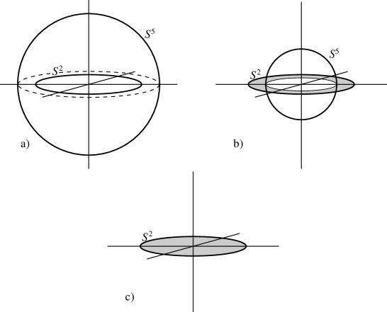
FIG. 2.: a) A small baryon vertex, at $r>r_{0}$: the $S^{5}$ baryon vertex is outside the $S^{2}$ of the vacuum brane (the vacuum brane is also extended in 123, while the baryon is not). b) The baryon $S^{5}$ contracted to $r<r_{0}$: a 3-brane (shaded) has been created. c) The $S^{5}$ has contracted to nothing, leaving a 3-brane baryon filling the $S^{2}$.

Looking globally at the two-sphere, we see that the D3-brane fills the part of the NS5-brane two-sphere which lies outside the D5-brane. But the space inside the NS5-brane is topologically flat; the radius of the five-sphere shrinks to zero inside. The D5-brane therefore is topologically unstable and can be shrunk to zero radius, leaving a D3-brane which fills the entire two-sphere inside the NS5-brane. Like the D5-brane which created it, this D3-brane is a particle in the four-dimensional spacetime; more precisely, it is a localized object whose size is of order $m^{-1}$. If the charged sources are taken to lie further apart than this, then they will connect to the D3-brane not directly but through F1-NS5 flux tubes; thus the baryon vertex behaves dynamically as we would expect in a confining theory.

The D5-brane baryon vertex in the ${\cal N}=4$ theory has no preferred size or energy. Here, the D3-brane actually represents a physical excitation of definite size and mass. The mass is

$$\frac{\mu_{3}}{g}\int_{B^{3}}d^{3}x\,e^{-\Phi}{G^{1/2}_{\rm string}} = \frac{\mu_{3}R^{2}}{g}\int_{0}^{r_{0}}dw\,\frac{4\pi w^{2}}{(r_{0}^{2}+\rho^{\prime 2}_{\rm c}-w^{2})}$$ (154)

$$\approx N\frac{m\sqrt{gN}}{2\pi^{3/2}}\ln(gN)\ .$$ (155)

Note that this diverges, due to a net factor $Z^{1/2}$ in the integrand, until the near-shell form is taken into account. The result is a factor of $N$ times ’t Hooft scaling, as would be expected.

To see directly that the D3-ball is a baryon vertex, note that the NS5-brane world-volume action includes a Chern-Simons term

$$\int F_{\it 2}\wedge F_{\it 2}\wedge B_{\it 2}\ .$$ (156)

This is the $S$-dual of the term

$$\int F_{\it 2}\wedge F_{\it 2}\wedge C_{\it 2}$$ (157)

in the D5-brane action, which is familiar as it implies that a world-volume gauge instanton is a dissolved D1-brane. The D3-brane ending on the NS5-brane is a magnetic monopole source for $F_{\it 2}$ (the $S$-dual of a familiar fact for D3- and D5-branes), while the dissolved D3-branes become $N$ units of $F_{\it 2}$. Under $\delta B_{\it 2}=d\chi_{\it 1}$,

$$\delta\int F_{\it 2}(\mbox{monopole})\wedge F_{\it 2}(\mbox{dissolved})\wedge B_{\it 2}=-\int dF_{\it 2}(\mbox{monopole})\wedge F_{\it 2}(\mbox{dissolved})\wedge\chi_{\it 1}\ .$$ (158)

This violation, proportional to the number of dissolved D3-branes, must be offset by $N$ fundamental strings ending at the D3-NS5 junction.

Note that this now also explains the ${\bf Z}_{N}$ quantum numbers of the flux tubes. If we place $N$ flux tubes close and parallel to each other, pair-creation of these D3-branes can occur. This allows the flux tubes to annihilate in groups of $N$.

Application of $S$-duality allows us to form the same construction for other similar vacua. Notice that the baryon vertex is always a D3-brane. However, the 5-brane on which it ends determines its properties. For example, if we are in the Higgs vacuum, the magnetic flux and its magnetic baryon form the $S$-dual of what we just considered. By contrast, the electric baryon is completely shielded: the $N$ fundamental string sources, which in the confining vacuum were forced to end on the D3-brane, are no longer forced to do so, since they may end anywhere on the D5-brane. This is of course consistent with field theory expectations.

Now let us consider some other vacua. Suppose that we take a vacuum where the classical unbroken gauge group was $SU(N/k)$, with $k\ll\sqrt{N}$ a small divisor of $N$. Since only the $SU(N/k)$ confines, and since a fundamental representation of the $SU(N)$ parent breaks up into $k$ copies of the fundamental representation of $SU(N/k)$, we should expect that $N$ sources would now be joined by not one but $k$ different baryon vertices. To see this in the supergravity is straightforward. The relevant vacuum is given by $k$ coincident NS5-branes, so when the D5-brane baryon vertex of ${\cal N}=4$ crosses the NS5-branes, $k$ D3-branes are created. Each of these carries $N/k$ units of string charge (since each NS5-brane has $N/k$ units of D3-brane charge) and so $N/k$ strings must end on each of them. On the other hand, the $k$ D3-branes are not bound together and may be separated spatially from one another. Each one represents a separate, dynamical, massive baryon vertex of $SU(N/k)$. Note also that pair creation of these objects ensures that the electric flux tubes in this vacuum carry only ${\bf Z}_{N/k}$ quantum numbers.

C Flux Tubes: A Second Pass

Here we will look at Coulomb vacua to understand how the baryons and strings behave, and obtain the correct flux tube quantum numbers.

We have already noted the flux tubes present when the vacuum is massive — that is, when the classical vacuum is given by $k$ copies of the $N/k$-dimensional representation of $SU(2)$. The baryons ensured that the electric flux tubes carry flux in ${\bf Z}_{k}$ and the magnetic or dyonic flux tubes have charge in ${\bf Z}_{N/k}$.

Let us consider instead a general Coulomb vacuum, given by choosing $p_{i}$ copies of the $q_{i}$-dimensional representation, with $\sum p_{i}q_{i}=N$. The unbroken gauge group is $[U(p_{1})\times U(p_{2})\times...\times U(p_{k})]/U(1)$, corresponding to $p_{i}$ D5-branes of $AdS$ radius proportional to $q_{i}$. Let $r$ to be the greatest common divisor of the $p_{i}$, and $s=\gcd(q_{i})$. Simple field theoretic arguments then determine the properties of possible flux tubes. The topology of the breaking pattern of the gauge group permits magnetic flux tubes to carry a ${\bf Z}_{s}$ charge, while the massive $W$-bosons of the theory will break all electric flux tubes down to those carrying a ${\bf Z}_{r}$ charge.

How do we see these flux-charges in the supergravity? For the magnetic flux, it is straightforward. Consider a collection of $k$ magnetic flux tubes. A magnetic flux tube can be moved with impunity from one D5-brane to another, since two flux tubes on different D5-branes can be connected by a D1-string in the radial direction, corresponding to a magnetic gauge boson. A magnetic baryon vertex connecting to a D5-brane of radius $q_{1}$ can remove or add $q_{1}$ flux tubes from the $k$ that we started with. Since we may move all the flux tubes from the first group of D5-branes to the second group, we may also remove any multiple of $q_{2}$ flux tubes from our collection. Removing $q_{i}$ flux tubes in any combination, we are left with a number $\hat{k}$ with $0\leq\hat{k}<\gcd(\{q_{i}\})$. This confirms what we set out to prove.

To see the charges of the electric flux tubes requires $S$-duality, which in not understood for the general Coulomb vacuum. However, we conjecture that the $\tau\to-1/\tau$ transformation acts in a simple way in an important subclass of the vacua. In particular, consider those classes of vacua where all $\{p_{i}\}$ are distinct integers and all $\{q_{i}\}$ are distinct integers. In this case we claim that the $S$-dual of this vacuum is that with $q_{i}$ NS5-branes of radius $p_{i}$. This is of course consistent with the known transformation of the massive vacua [5], for which $p_{1}q_{1}=N$. The $S$-dual of the argument in the previous paragraph then shows that the electric flux tubes for these vacua is indeed ${\bf Z}_{r}$. Indeed, this is our main evidence for the conjecture.

If the $p_{i}$ or the $q_{i}$ are not distinct integers, then the $S$-duality transformation we have suggested is ambiguous. We do not know what happens in this case, either in field theory or in supergravity.

D Domain Walls

Since the theory has many isolated vacua, it also has a large number of domain walls which can separate two spatial regions in different vacua. If the walls are spatially uniform then they may be BPS saturated [61, 62].

Between the oblique confining vacuum represented by a $(1,1)$ 5-brane sphere and the confining vacuum represented by an NS5-brane, there must be a BPS domain wall which carries off one unit of D5-brane charge. We may therefore conjecture that a BPS junction of three 5-branes — the NS5-brane sphere for $x^{1}>0$, the $(1,1)$ 5-brane sphere for $x^{1}<0$, and a D5-brane at $x^{1}=0$ which fills the two-sphere — describes this domain wall. That is, the world-volume of the D5-brane is the $023$-plane of the domain wall times the three-ball spanning the two-sphere. At small $g$ the NS5-brane and the $(1,1)$ brane are nearly coincident (their $AdS$ radius and orientation on the $S^{5}$ differ only at order $g$) and the effect of the D5-brane on the much denser NS5-brane is very small.

We can see that this reproduces some known properties of the domain wall. First [61, 62], the flux tubes of the theory (F1 strings) obviously can end on the domain wall (a D5-brane). Furthermore, consider dragging a $(1,1)$ dyonic string, representing a dyonic source in the gauge theory, across the wall. For $x^{1}<0$, the dyon is screened; it can end happily on the $(1,1)$ 5-brane. For $x^{1}>0$, the dyon is confined; its monopole charge ends on the NS5-brane, but its electric charge must join onto a flux tube — an F1-NS5 bound state — which in turn ends on the D5-brane domain wall. Finally, note that we may dissolve an $N$-string vertex (a D3-brane) into this domain wall (a D5-brane), leaving $N$ strings which end on the wall and are free to move around on it. If we then permit this domain wall to annihilate with an antidomain wall with no strings attached, then the annihilation will leave a D3-brane behind on which the strings may end, as in the well-known process described in [63].

More generally, if for $x^{1}<0$ the system is in the phase corresponding to a $(c,d)$ 5-brane, and for $x^{1}>0$ it is in the phase corresponding to a $(c^{\prime},d^{\prime})$ 5-brane, then a $(c-c^{\prime},d-d^{\prime})$ 5-brane must fill the 2-sphere where they meet. In general the branes on the right and left have different orientations and radii, and so must bend as they meet as depicted in figure 3.

FIG. 3.: Triple 5-brane junction, corresponding to a domain wall. Depicted is $z(x^{1})$; the full geometry is obtained by translating in $x^{2,3}$ and rotating in the transverse $SO(3)$ symmetry. At $x^{1}<0$ the system is in the vacuum corresponding to 5-brane A; at $x^{1}>0$ it is in the vacuum corresponding to 5-brane B, with different radius and orientation. The domain wall lies in the shaded plane $x^{1}=0$ and is a 5-brane of type C. The bending of branes A and B is described by the BPS equation (169).

When the left and right phases involve multiple spheres, there will be a more complicated domain wall, constructed from multiple triple 5-brane junctions.

To discuss the domain wall tensions quantitatively we need the kinetic term for the collective coordinate $z=2\pi\alpha^{\prime}\phi$. This arises in the Born-Infeld action, from

$$G_{\mu\nu}(\mbox{induced})=G_{\mu\nu}+G_{mn}\partial_{\mu}x^{m}\partial_{\nu}x^{n}\ .$$ (159)

Then

$$\frac{S}{V}=-\frac{\mu_{5}}{2g}2\pi\alpha^{\prime}\int d^{2}\xi\,G_{\perp}^{1/2}(F_{ab}F^{ab})^{1/2}\eta^{\mu\nu}\partial_{\mu}x^{m}\partial_{\nu}x^{n}=-\frac{n}{2\pi g}\eta^{\mu\nu}\partial_{\mu}\bar{\phi}\partial_{\nu}\phi\ .$$ (160)

This gives the Kähler potential $K=n\bar{\Phi}\Phi/2\pi g$. This is the same as Eq. (99) for the classical gauge theory, but by an $SL(2,{\bf Z})$ transformation one can show that it holds for all $(c,d)$. This makes sense, as the main kinetic effect comes from the D3-branes, which are self-dual. With this normalization the potential (106) implies the superpotential

$$W=\frac{1}{4\pi g}(i\frac{4\sqrt{2}}{3M}\Phi^{3}+mn\Phi^{2})\ .$$ (161)

as in Eq. (99). At the nonzero stationary point this takes the value

$$W\to-\frac{m^{3}n^{3}}{96\pi gM^{2}}\ .$$ (162)

For a multi-brane configuration it is summed over $I$.

We cannot rule out an additional additive contribution to this superpotential, although from our semiclassical reasoning we know that any such contribution must be subleading in the Higgs vacuum and others containing only large D5-branes. Field theory also suffers from the same ambiguity [8]. Up to these additive contributions, the field theory and supergravity agree. Consider the massive vacuum corresponding to $p$ D5 branes of radius $q$; for this vacuum $M=p$. Using [7], it is easy to obtain a slight generalization of [8] (adjusted to match our conventions, and with the function $A(\tau,N)$ in Eq. (5) of [8] set to zero)

$$W={m^{3}N^{2}\over 24g_{{\rm YM}}^{2}}\left[E_{2}(\tau)-{q\over p}E_{2}\left({q\over p}\tau\right)\right]\to{m^{3}N^{2}E_{2}(\tau)\over 96\pi g}-{m^{3}N^{3}\over 96\pi gp^{2}}\ .$$ (163)

Here $E_{2}$ is the second Eisenstein series, and we have used Eq. (108) and $E_{2}(i\infty)=1$. Note the first term is $p$ independent and is subleading for $p\ll\sqrt{N}$. For the massive vacuum given by $q$ $(1,k)$ 5-branes of radius $p$, $k\ll p$, in which $M=q(\tau+k)$, the formula is

$$W={m^{3}N^{2}\over 24g_{{\rm YM}}^{2}}\left[E_{2}(\tau)-{q\over p}E_{2}\left({q\over p}(\tau+k)\right)\right]\ ,$$ (164)

but since Eqs. (109) applies and $xE_{2}(x)=x^{-1}E_{2}(-x^{-1})+(6i/\pi)$,

$$W\to{m^{3}N^{2}E_{2}(\tau)\over 96\pi g}-{m^{3}N^{3}\over 96\pi gq^{2}(\tau+k)^{2}}\ .$$ (165)

The first term in this expression is the same as in the D5-brane vacua, so field theory and supergravity agree up to a classically-subleading $M$-independent function.

For a supersymmetric domain wall between two phases, the tension is

$$\tau_{\rm DW}=2|\Delta W|\ =\frac{|m^{3}|}{48\pi g}\left|\sum_{I\,\rm left}\frac{n_{I}^{3}}{M_{I}^{2}}-\sum_{J\,\rm right}\frac{n_{J}^{\prime 3}}{M_{J}^{\prime 2}}\right|\ .$$ (166)

Let us consider two examples, to see that the 5-brane junction construction reproduces this tension. For both examples we take $g\ll 1$.

The first is the domain wall described above, between the confining and first oblique confining phase. The general result (166) becomes

$$\tau_{\rm DW}=\frac{|m^{3}|N^{3}}{48\pi g}\Bigl{|}(ig^{-1})^{-2}-(ig^{-1}+1)^{-2}\Bigr{|}\approx\frac{|m^{3}|g^{2}N^{3}}{24\pi}\ .$$ (167)

In the brane picture, the tension comes from the spanning D5-brane. This has three transverse and three longitudinal dimensions and so feels no warp factor, giving simply

$$\tau_{\rm DW}=\frac{4\pi r_{0}^{3}}{3}\cdot\frac{\mu_{5}}{g}=\frac{|m^{3}|g^{2}N^{3}}{24\pi}\ .$$ (168)

The agreement is quite beautiful, given the very different physics that has gone into the two calculations.

The second example is the domain wall between the confining and Higgs phases: a junction between an NS5-brane and a D5-brane, spanned by a (1,1) 5-brane. The NS5-brane is at much smaller radius than the D5-brane (by a factor $g$) and has much greater tension, so the predominant effect is that the D5-brane bends down to join the NS5-brane. The bending is described by the BPS equation

$$\partial_{1}\phi=\Omega\hskip 1.0pt\overline{\frac{\partial W}{\partial\phi}}\hskip 1.0pt$$ (169)

with $\Omega$ any phase. For $m$ real, $\Omega=-1$ gives a solution that passes through the origin and the nonzero stationary point, approximating to order $g$ the solution needed. The tension comes primarily from this bending,

$$\tau_{\rm DW}=\int_{0}^{\infty}dx^{1}\,\biggl{(}\frac{N}{2\pi g}|\partial_{1}\phi|^{2}+\frac{2\pi g}{N}|W_{\phi}|^{2}\biggr{)}\ .$$ (170)

In this case the general result (166) follows by construction

$$\tau_{\rm DW}=\frac{|m^{3}|N^{3}}{48\pi g}\ ,$$ (171)

where the superpotential in the confining phase is smaller by $O(g^{2})$. It will be an interesting exercise to show that the brane construction reproduces Eq. (166) in the general case, without assuming small $g$.

Note that a domain wall is the same as a baryon vertex extended in two additional directions. By analogy, we might expect the D5-brane three-ball which acts as a domain wall to be associated with passing a D7-brane through the NS5-brane. This suggests that D7-branes should be reexamined in the original $AdS_{5}\times S^{5}$ context.

E QCD-like vacua

It is amusing that ${\cal N}=1^{*}$ is rich enough to permit us to study a theory similar to QCD with heavy quarks. Suppose we consider a vacuum with a D5-brane of radius $n$ and one NS5-brane of radius $N-n$. Here we assume the usual condition on $n$, $n^{2}\gg gN$, but take $n\sim gN$, so the D5-branes have comparable $AdS$ radius to the NS5-brane. In the field theory this corresponds to a vacuum with a broken $SU(n)$ sector, a $U(1)$ vector multiplet, and a confining $SU(N-n)$ sector. Among the massive vector multiplets are spin-1 bosons, along with fermions and scalars, charged as $(\bf{\bar{n}},\bf{N-n})$ under $SU(n)\times SU(N-n)$. These are strings connecting the D5-brane to the NS5-brane. We will refer to these as ‘quarks’. Clearly these theories have no free quarks: the D5-NS5 strings cannot exist in isolation, since they cannot actually end on the NS5-brane, and instead must be connected to a flux tube. Note that the $SU(n)$ acts as a sort of flavor group for the quarks (analogous to broken weak isospin), and we will refer to its massive adjoint representation as ‘flavor’ gauge multiplets.

In order that the supergravity solution be valid, we must have $n\gg(gN)^{1/2}$. When $n=gN$, so that the D5 and NS5 sit at equal $AdS$ radii, the quark has mass of order

$$(\alpha^{\prime})^{-1}\int\sqrt{G_{00}G_{yy}r_{0}^{2}}d\zeta=r_{0}/\alpha^{\prime}=mn$$

which agrees with field theory. However, it is easy to see that if $n$ is smaller than $gN$, the quark retains mass $\sim mgN$; indeed, as an extreme, note that if a D3-brane sits exactly at $r=0$, corresponding to $(gN)^{1/2}\ll n\ll gN$, the quark mass is just proportional to the coordinate length of the string, $mgN$. We therefore see signs that the physical ‘constituent’ masses of the quarks can be much larger than their current values. Of course the quarks are never light compared to $m$.

We can see easily that QCD-like theories have no stable flux tubes due to quark pair production. Recall that we measure the potential $V(L)$ between two electric sources by hanging a probe string by its ends from the $AdS$ boundary, with the ends a distance $L$ apart. Take $L\gg\ m^{-1}(gN)^{-1/2}$; then in the absence of the D5-brane, the probe would bind to the NS5-brane forming a confining flux tube between the sources. In the presence of the D5-brane, however, pair production of the D5-NS5 strings can occur. This breaks the flux tube, which shrinks away allowing the quark to screen the source. The probe string ends up as two strings a distance $L$ apart, each attached to the D5-brane. Note however that if we take $n\gg gN$, the quarks become very heavy, and the time scale for their pair production becomes very long. In this limit the confining flux tubes are metastable.

Low-lying quark-antiquark mesons are not stable in this theory. Highly excited mesons are represented by two D5-NS5 strings joined by a long F1-NS5 flux tube. However, as the mesons deexcite by emission of glueballs (either supergravity or string states), it eventually becomes energetically preferable for them to decay to a D5-D5 string, bypassing the NS5-brane altogether. In short, the lowest lying mesons between two quarks always mix with and decay to a massive, but lighter, flavor particle, in a vector multiplet of the broken $SU(n)$ group. (Indeed this almost happens in nature; charged pions decay through isospin gauge multiplets, although not because those gauge bosons are light but because they couple to light leptonic states — which could also be represented here, if there were a need.)

Baryons, on the other hand, carry a conserved charge and are both stable and interesting. $N-n$ D5-NS5 strings can end on a D3-brane filling the NS5-brane two-sphere, forming an object whose mass can be computed. If we arrange for a more complicated spectrum of quarks by choosing to use multiple D5-branes of various radii, then there are processes by which baryons can be built from quarks of different masses, and can decay by emission of flavored mesons (or the corresponding gauge multiplets of the ‘flavor’ group.) Scattering of baryons, or of baryons and antibaryons, could also be studied. In addition, it is possible that these baryons have residual attractive short range interactions (different from the physical case in that they are dominated by the ‘flavor’ gauge multiplets) which can cause them to form nuclei. It would be amusing to look for such baryon-baryon bound states. Furthermore, these baryons and nuclei carry $U(1)$ gauge charges, and in some vacua there are lepton-like objects which presumably can combine with them to form atoms.

We cannot resist mentioning one more possibility, although it admittedly may not be realized. Namely, our baryons act as D0 branes in spacetime, and our domain walls as D2-branes (their structure in the extra dimensions is identical, so we suppress it.) While we are not used to thinking of baryons as places where strings can end, this is quite natural if there are no light quarks; if all quarks are heavy then short flux tubes are stable, and physical baryons can be linked by them. Turning on condensates of these flux tubes makes the positions of the baryons noncommuting (note these branes have no massless world-volume gauge fields, but still have massless scalars), and through the Kabat and Taylor mechanism [15], an assembly of baryons can be arranged into a spherical domain wall! Thus the properties of the gauge theory recapitulate the method we have used to solve it. In practise, one should try to implement this process physically, through Myers’ mechanism [14]. Here we have a difficulty, as the required three-form potential is a massive state, a glueball which couples to domain walls [64], so we cannot create a long-range field to induce a dipole charge. However, there may be ways to circumvent this problem, and create this effect as a thought experiment or even in a lattice simulation, where hints of domain walls have been observed [65].

F Condensates

With the naked singularity banished, the coefficients of the normalizable terms in the supergravity fields, and so the dual condensates, become calculable. We have already determined the superpotential in our discussion of domain walls, and in principle the condensates can be determined directly from this function. The full field theoretic superpotential, and corresponding condensates, are also known [8]. However there are subtleties [39, 66], and our understanding is only partial.

The condensates of the operators $\lambda\lambda$, ${\rm tr}[\Phi_{1},\Phi_{2}]\Phi_{3}$ and $m_{i}{\rm tr}\Phi_{i}\Phi_{i}$ are all related by the chiral anomaly and operator mixing. A linear combination of these must couple, by the $AdS$/CFT correspondence, to the mode of $G_{\it 3}$ which falls off as $1/r^{3}$ in invariant units, which we have identified in Eq. (66). More generally, higher modes of $G_{\it 3}$ should give the expectation values of all of the chiral operators $\lambda\lambda\phi^{k}+\cdots$. For the lowest mode of $G_{\it 3}$, Eq. (123) for $\omega_{2}$ gives the $m$ and phase dependent parts as

$$Mr_{0}^{3}\propto\frac{m^{3}N^{3}}{M^{2}}\ .$$ (172)

For multiple shells, superposition gives

$$m^{3}\sum_{I}\frac{n_{I}^{3}}{M_{I}^{2}}\ .$$ (173)

Note that there are two $SO(3)$-invariant fermion bilinears, namely $\sum_{i=1}^{3}\lambda_{i}\lambda_{i}$ and $\lambda_{4}\lambda_{4}$. These correspond to the polarization tensors $\epsilon_{i\bar{\jmath}\bar{k}}$ and $\epsilon_{ijk}$, which have equal overlap with the actual field $\epsilon_{w^{1}w^{2}w^{3}}$.

In the Higgs vacuum, and other vacua with only large D5-branes, all condensates can be described semiclassically. The expectation values for ${\rm tr}[\Phi_{1},\Phi_{2}]\Phi_{3}$ and $m_{i}{\rm tr}\Phi_{i}\Phi_{i}$ are known, and their $m$, $n$ and $M$ scaling agrees with (173). In the confining cases, however, the situation is more subtle, since these operators have condensates of different sizes and since the gluino bilinear is also expected to play a role. We note the following facts. First, careful examination of the field theory superpotential given in [7, 8] reveals no obvious linear combination of the operators whose expectation values would have this property — except the second term in the superpotential itself, as discussed in section VII.D. Second, there is every indication from our study of domain walls that the second term in the superpotential, proportional to the two-sphere volume times the 5-brane’s charge under $*G_{\it 3}$, measures the dipole moment of the 5-branes. Naturally, the lowest normalizable mode of $G_{\it 3}$ couples to the lowest allowable 5-brane multipole moment, which is indeed a magnetic dipole. We therefore speculate that perhaps the $ijk$ components of $G_{\it 3}$ couple to this part of the superpotential, and to the worldsheet instantons which we will discuss in section VII.G below.

In any case, the supergravity clearly shows that there are expectation values for some dimension-three operators which classically would have had vanishing vevs. It also shows these vevs differ from one confining vacuum to the next. These qualitative features certainly agree with field theory.

The chiral operators $F^{2}\phi^{k}$ are determined by the dilaton background. The dilaton is nontrivial and is obtained from

$$\nabla^{2}\Phi=\frac{2\pi gr_{0}^{4}|M|^{2}}{NR^{2}}\delta^{3}(y)\delta(w-r_{0})+\frac{g^{2}}{12}{\rm Re}(G_{mnp}{G}^{mnp})\ .$$ (174)

The first term comes from the coupling of the dilaton to the 5-brane through the Born-Infeld action. The second is directly from the coupling to the bulk fields. Taking the value of $r_{0}$ appropriate to a single shell of quantum numbers $M$, and integrating over a volume of order $r_{0}^{6}$, both terms are of order $m^{6}R^{2}r_{0}^{4}$ and must be retained. One can argue that they must cancel in the dilaton monopole, which gives the expectation value of the derivative of the Lagrangian with respect to the coupling; this must vanish in a supersymmetric vacuum. Many of the higher operators $F^{2}\phi^{k}$ are also highest components of superfields, and for them a similar argument should apply. We have not yet shown this cancellation directly for the background (174), and it is possible that there are subtleties. It is a challenge to include this varying dilaton in the full nonlinear treatment of supergravity.

G Instantons

At weak coupling, many quantities in ${\cal N}=4$ Yang-Mills theory receive contributions from instantons. Holomorphic objects can be written as an instanton expansion, given by an infinite series in powers of the parameter $q=e^{2\pi i\tau}$. This expansion is not useful at strong coupling, but in that case the same objects can typically be reexpressed, using a modular transformation, in terms of $\tilde{q}=e^{-2\pi i/\tau}$ (or some other $SL(2,{\bf Z})$ variant.) In string theory, both in perturbation theory for flat D3 branes and in the $AdS_{5}\times S^{5}$ language, D-instantons [D-($-1$) branes], whose action is $2\pi/g$, play the role of these field theory instantons. For large $g$ one uses an expansion in magnetic D-instantons, with action $2\pi g$, or more generally in dyonic D-instantons.

In ${\cal N}=1^{*}$, the situation is slightly different. Consider first weak ’t Hooft coupling, such that the strong coupling scale $\Lambda$ is much less than $m$. In this case the Higgs vacuum has a superpotential which is an expansion in $q=e^{2\pi i\tau}$, but the superpotential of the confining vacuum has an expansion in $q^{1/N}$. The $1/N$ in the exponent is responsible, in the $m\to\infty$ limit, for $SU(N)$ Yang-Mills having $N$ vacua, related by $\theta\to\theta+2\pi k$. It has long been suggested that this behavior implies the existence of fractional instantons, carrying $1/N$ units of instanton charge, which, unlike instantons themselves, remain important in the large $N$ limit. Some evidence for these objects has been found in MQCD [67] (note that these are distinct from similar objects which require compactification of a dimension of spacetime for their existence) and there is even a claim that they have been seen in lattice nonsupersymmetric Yang-Mills [68].

We might hope to find such objects here, but for the same reason that $\Lambda\sim m$, we cannot do so, for $q^{1/N}$ is of order one, and the fractional-instanton expansion fails. We also cannot use the magnetic instanton expansion, since $g\ll 1$. But remarkably, as can be inferred from the results of [8], there is yet another expansion, one which is dual, in the sense of $gN\leftrightarrow(gN)^{-1}$, to the expansion in fractional instantons.

In particular, Dorey and Kumar show that the superpotential for the confining vacuum is proportional to

$$E_{2}(\tau)-{1\over N}E_{2}\left(\tau\over N\right)$$ (175)

where $E_{2}$ is the second Eisenstein series. For large imaginary arguments, $E_{2}(z)$ can be written as an expansion in $e^{2\pi iz}$. The first term in (175) can therefore be interpreted as a sum over ordinary instantons. The second term, by contrast, cannot be expanded in this way, since $|\tau/N|\ll 1$. However, since $N/\tau$ is large and imaginary, we may make progress as in [8] by using the anomalous modular transformation

$$E_{2}(z)={1\over z^{2}}E_{2}\left(-{1\over z}\right)+{6i\over\pi z}\ .$$ (176)

from which we learn that the second term in Eq. (175) dominates the first and that it can be expanded in power of $e^{-2\pi iN/\tau}=e^{-2\pi gN}$. This is an expansion in a small quantity, and we need only provide an interpretation for it.

This is not difficult to obtain, for an NS5-brane of the form $S^{2}$ times Minkowski space permits the string world-sheet to wrap the $S^{2}$, producing instantons. From the metric (142) the proper area of the NS5-brane sphere times the tension of the fundamental string is minimized by

$$(4\pi r_{0}^{2}){R^{2}\over 2r_{0}\rho_{c}}{1\over 2\pi\alpha^{\prime}}={R^{4}\over 2\alpha^{\prime 2}}=2\pi gN$$ (177)

which is just as required to explain the expansion in the superpotential. As a check, note that if we repeat the calculation for a vacuum with $q$ coincident spheres, both the area of the spheres and the exponent in the field theory are reduced by a factor $q$. For the Higgs vacuum, the metric and dilaton in Eqs. (139) and (141) imply the area of the D5-sphere times the tension of a D1 brane goes at small $\rho$ to

$$\frac{R^{4}}{2g^{2}\alpha^{\prime 2}}=2\pi N/g\ .$$ (178)

Since the Higgs vacuum superpotential is proportional to [8]

$$E_{2}(\tau)-{N}E_{2}\left(N\tau\right)$$ (179)

we may again interpret the second term (now much smaller than the first term, except for its leading $\tau$-independent contribution) as an expansion in D1-instantons wrapping the D5-brane two-sphere.

It would be interesting to find a string theory interpretation for the coefficients in the expansion of of the superpotential, and especially for the anomalous term in the modular transformation of $E_{2}$.

H Glueballs and Other Particle States

The spectrum of states in this theory is complicated, and we do not yet have a physical understanding of its features. We will outline its structure and point out some puzzles and problems which must be solved in future.

First, there is already surprising structure in the ${\cal N}=4$ theory in the vacuum with $Z$ given by Eq. (102), where the D3-branes form a 2-sphere of radius $r_{0}$. The typical warp factor in the region $r\sim r_{0}\sim mN(g)\alpha^{\prime}$ is $Z\sim R^{4}/r_{0}^{4}$. A supergravity state then has typical $k_{\mu}$ given by [69]

$$G^{\mu\nu}k_{\mu}k_{\nu}\sim G^{mn}k_{m}k_{n}$$ (180)

so that

$$k_{\mu}\sim Z^{-1/2}k_{m}\sim\frac{r_{0}}{R^{2}}\sim mg^{\pm 1/2}N^{1/2}\ .$$ (181)

where the minus (plus) sign applies for the D3-sphere radius appropriate to the Higgs (confining) vacuum. Immediately we have a puzzle. The semiclassical field theory of this ${\cal N}=4$ vacuum would have led us to expect physics from the $W$-bosons whose masses lie between the scales $m$ and $Nm$. There are also monopoles of masses $m/g$ and $Nm/g$. These states are present on the supergravity side as F- and D-strings stretched between the D3-branes. But there is no sign of gauge theory states with masses given in the previous equation. The situation is not improved by consideration of excited string states in the bulk, for which one has similarly

$$G^{\mu\nu}k_{\mu}k_{\nu}\sim 1/\alpha^{\prime}$$ (182)

and

$$k_{\mu}\sim Z^{-1/4}\alpha^{\prime-1/2}\sim\frac{r_{0}}{R\alpha^{\prime 1/2}}\sim mg^{\pm 1/2}N^{1/2}\times(gN)^{1/4}\ ,$$ (183)

an odd-looking scale.

Now, what changes when the D5- or NS5-brane charge is added? For the D5-brane, essentially nothing happens to these arguments. This is despite the fact that a magnetic flux tube has formed, with a tension whose square root is given by Eq. (181) with the minus sign. Presumably the details shifts around slightly, and of course the massless photons of the D3-branes now develop mass of order $m$, but apparently the spectrum is otherwise little changed.

For the NS5-brane, the situation is more subtle. The electric flux tube has a tension whose square root is given, as in the D5 case by Eq. (181), now with the plus sign. But in addition, unlike the D5-brane, the NS5-brane has a throat region. If we consider a vacuum with several coincident NS5-branes, then the throat region is reasonably well understood, since it can be described in conformal field theory in the region where the string coupling is small [50]. From this it is known that supergravity states get string-scale masses from the coupling to the throat geometry. Using the metric (136) in the calculation (182) gives

$$k_{\mu}\sim r_{0}^{1/2}\rho_{\rm c}^{\prime 1/2}R^{-1}\alpha^{\prime-1/2}\sim\frac{r_{0}}{R^{2}}\sim mg^{1/2}N^{1/2}\ .$$ (184)

This applies to both supergravity and excited string states. Notice that this is the same scale as for supergravity states in the bulk, and for the string tension.

Unfortunately, the confining vacuum has only one NS5-brane, and there is a long-standing controversy over this object, reflecting the difficulty of doing any reliable calculations in its presence [56]. There are disputes over whether the throat and its region of strong coupling even exist. In any case, neither supergravity nor conformal field theory is reliable, and we simply do not know what the spectrum will do in this regime. We note this may hint at a profound obstacle to using string theory as a practical computational tool in QCD.

In both the D5 and NS5 cases, there is one more class of light states, arising from the massless gauge fields on the 5-brane. Relative to the bulk states, the magnetic field on the D5-brane reduces the velocity of open string states by a factor of the dimensionless field, $v\sim(N/g)^{-1/2}$: restoring $F_{\mu\nu}F^{\mu\nu}$ and $F_{\mu a}F^{\mu a}$ to the brane action, one finds that the latter is multiplied by $v^{2}$. The mass gap is reduced by the corresponding factor, and so is simply

$$k_{\mu}\sim m\ .$$ (185)

This agrees with the classical result, since these are the $W$ bosons and this is the scale of $SU(N)$ breaking. Meanwhile, the NS5-brane has a normalizable zero mode [70], which gives rise to the massless vector required by $S$-duality to the D5-brane. We assume that this mode survives when D3-branes are dissolved in the NS5-brane. Then

$$G^{\mu\nu}k_{\mu}k_{\nu}\sim G^{w^{1}w^{1}}k_{w^{1}}k_{w^{1}}\ ,$$ (186)

and

$$k_{\mu}\sim\frac{r_{0}\rho_{\rm c}^{\prime}}{R^{2}}k_{w^{1}}\sim\frac{\rho_{\rm c}^{\prime}}{R^{2}}\sim m\ .$$ (187)

Again we find a lighter branch of states localized at the brane. By analogy to the Higgs vacuum, one might interpret them as massive magnetic gluons, but in the NS system they are not open strings but rather closed string states in localized wavefunctions on the throat. Most of them carry $SO(3)$ quantum numbers and are therefore not seen in ${\cal N}=1$ Yang-Mills theory. Some or all of the remainder may mix with bulk states, as we discuss below.

Before doing so, we note that all of the masses we have obtained in the confining vacuum are consistent with ’t Hooft scaling, as they are proportional to $m$ times a power of $gN$. This is pleasing, although it means of course that all of the states merge and mix as $gN$ is taken small, making any quantitative computations in this regime essentially irrelevant for ${\cal N}=1$ Yang-Mills.

Let us note one important interplay between the open and closed string states. There would appear to be one unbroken $U(1)$ gauge group per (noncoincident) brane, from the world-sheet gauge field on each brane. For an $SU(2)$ representation given by the sum of $k$ distinct irreducible blocks, $SU(N)$ is broken to $U(1)^{k-1}$. On the string side there are $k$ D5-spheres and so apparently a $U(1)^{k}$. In fact, one $U(1)$ should be lifted by the coupling to the bulk states. We have not understood all the details, but will indicate the ingredients. There is a massless tensor in $3+1$ dimensions, with the field $B_{\mu\nu}$ independent of $x^{m}$. Its kinetic term is

$$\int d^{10}x\,\sqrt{G}H_{\mu\nu\lambda}H^{\mu\nu\lambda}=\int d^{4}x^{\mu}\,\eta^{\mu\mu^{\prime}}\eta^{\nu\nu^{\prime}}\eta^{\lambda\lambda^{\prime}}H_{\mu\nu\lambda}H_{\mu^{\prime}\nu^{\prime}\lambda^{\prime}}\int d^{6}x^{m}\,Z^{2}\ .$$ (188)

The $x^{m}$ integral converges both at the branes and at infinity, so this is a discrete state. By itself, the coupling of this field to $F_{\mu\nu}$ in the Born-Infeld action would generate a mass for one linear combination of $U(1)$’s via the Higgs mechanism. However, the field $C_{\mu\nu}$ also has a zero mode, seemingly lifting a second $U(1)$. The actual story must be more complicated, with the bulk Chern-Simons term playing a role, because from the point of view of a single brane this would be simultaneous electric and magnetic Higgsing, an impossibility.

VII Extensions

A Unequal Masses

Now we consider the general ${\cal N}=1$ case, three masses not necessarily equal. Examination of the classical $F$-term equations (6) suggest use of the coordinates

$$z^{1} = \sqrt{m_{2}m_{3}}\,\chi\cos\theta\ ,$$ (189)

$$z^{2} = \sqrt{m_{1}m_{3}}\,\chi\sin\theta\cos\phi\ ,$$ (190)

$$z^{3} = \sqrt{m_{1}m_{2}}\,\chi\sin\theta\sin\phi\ .$$ (191)

We will study the potential with the Ansatz that $\chi$ is constant and also that $F_{\theta\phi}=\frac{1}{2}n\sin\theta$. We insert this into the potential (93). Noting that

$$\det G_{\perp} = 4\tilde{m}|m_{1}m_{2}m_{3}\chi^{4}|Z\sin^{2}\theta\ ,$$ (192)

$$\tilde{m} \equiv |m_{1}|\cos^{2}\theta+|m_{2}|\sin^{2}\theta\cos^{2}\phi+|m_{3}|\sin^{2}\theta\cos^{2}\phi\ ,$$ (193)

$$T_{mnp}x^{m}dx^{n}\wedge dx^{p} = |m_{1}m_{2}m_{3}|(|m_{1}|+|m_{2}|+|m_{3}|)\chi\bar{\chi}^{2}\ ,$$ (194)

$$T_{i\bar{\jmath}\bar{k}}\hskip 1.0pt\overline{T}\hskip 1.0pt_{\bar{l}jk}z^{i}\bar{z}^{\bar{l}} = 2\tilde{m}|m_{1}m_{2}m_{3}\chi^{2}|\ ,$$ (195)

the potential becomes

$$-\frac{S}{V}=\frac{4|m_{1}m_{2}m_{3}|}{\pi gn(2\pi\alpha^{\prime})^{4}}\frac{|m_{1}|+|m_{2}|+|m_{3}|}{3}|M\chi^{2}-2\pi\alpha^{\prime}in\chi/2\sqrt{2}|^{2}\ .$$ (196)

This has a supersymmetric minimum at $\chi=2\pi\alpha^{\prime}in/2\sqrt{2}M$. The two-sphere is now an ellipsoid with axes

$$\frac{\pi\alpha^{\prime}n}{|M|}\sqrt{|m_{2}m_{3}|}\ ,\quad\frac{\pi\alpha^{\prime}n}{|M|}\sqrt{|m_{1}m_{3}|}\ ,\quad\frac{\pi\alpha^{\prime}n}{|M|}\sqrt{|m_{1}m_{2}|}\ .$$ (197)

When $m_{3}\to 0$ with $m_{1}=m_{2}$ fixed, we obtain ${\cal N}=2$ Yang-Mills; here the ellipsoid degenerates into a line of length $m_{1}$. This is very easy to understand, classically, for the Higgs vacuum. ${\cal N}=2$ Yang-Mills with a massive hypermultiplet has a moduli space, which classically is just given by the positions of D3-branes (suitably modified so that they can only move in two dimensions — this remains to be understood in our present context.) On this space is a single point where there are $N-1$ massless electrically charged particles, from the hypermultiplet. At this point, the $N$ D3-branes are arranged in a line. From the classical equations, it is easy to see that an ${\cal N}=2$ breaking mass parameter for the vector multiplet causes this line to become a noncommutative ellipsoid analogous to the sphere of [15]. In addition, the electromagnetic dual of this transition corresponds to a well-known fact, both in field theory [71, 72, 73] and in MQCD [62, 74, 75, 76], concerning the breaking of pure ${\cal N}=2$ Yang-Mills to ${\cal N}=1$. The moduli space of ${\cal N}=2$ has an associated Seiberg-Witten auxiliary Riemann surface of genus $g$. There are $N$ special isolated points on the moduli space where $N-1$ mutually local dyons become massless, and the Riemann surface completely degenerates. In this degeneration, the $N$ handles of the surface join along a singular line segment. The addition of a mass parameter breaking ${\cal N}=2$ supersymmetry to ${\cal N}=1$ engenders a transition whereby the $N$ handles join to form a single surface of genus zero: the line segment opens up into a closed curve. In M theory this is represented by a multigenus M5-brane making a transition to a genus zero M5-brane. Here we see signs of a similar phenomenon; the 3-branes which represent the moduli space of the ${\cal N}=2$ theory presumably align along a line segment, then join and expand to form an NS5-brane ellipsoid.

By contrast, when $m_{1}=m_{2}\to 0$ with $m_{3}$ fixed, the ellipsoid becomes a disk while its overall size shrinks to zero. In the field theory, one expects an infrared fixed point, and indeed the supergravity should go over smoothly to the kink solution of [37] and at small $r$ to the ten-dimensional space of [77]. Presumably the $G_{\it 3}$ background in [77] is related to the linearized one we have obtained in Eq. (52), although we have not checked this.

It would be interesting to understand these connections in more detail, but we should note that our approximations will break down in these limits. We have seen that the 5-brane shell has a finite thickness, and we need this to be less than the shortest axis of the ellipsoid for our linearized approach to be consistent.

We note also that most of our results generalize easily to this case. The superpotential, the domain wall tensions and the condensates, are all related, as is the dipole moment of the 5-brane, to the volume of the ellipsoid $\propto m_{1}m_{2}m_{3}$. The flux tubes will presumably show signs of the extra metastable Regge trajectories seen in [73] by localizing on the ellipsoid, along the lines observed in MQCD in [75].

B ${\cal N}=0$

Let us make a few brief remarks about the nonsupersymmetric case, $m_{4}=m^{\prime}$ with $m_{1}=m_{2}=m_{3}=m$ kept equal. The potential is now

$$-\frac{S}{V}=\frac{4}{\pi gn(2\pi\alpha^{\prime})^{4}}\Biggl{\{}|M|^{2}|z|^{4}+\frac{2\pi\alpha^{\prime}n}{3\sqrt{2}}{\rm Im}\Bigl{[}(3mz\bar{z}^{2}+m^{\prime}z^{3})\hskip 1.0pt\overline{M}\hskip 1.0pt\Bigr{]}+\frac{(2\pi\alpha^{\prime}n)^{2}}{8}O(z^{2})\Biggr{\}}\ .$$ (198)

The quadratic term depends on the boundary conditions, as discussed at the end of section IV.A. Its general form is given by

$$O(z^{2})=\frac{1}{3}|z|^{2}\sum_{i=1}^{4}|m_{i}|^{2}+(L=2)\ .$$ (199)

In the absence of supersymmetry we must make a particular choice of the $L=2$ harmonic $\mu_{mn}$, defined in Eq. (87), which represents a traceless combination of masses for the scalar bilinears. This harmonic reduces the masses of some of the scalars, and if too large it can cause the gauge symmetry to break. However, it represents an adjustable parameter in the Lagrangian, so we are completely free to choose it in such a way that it preserves a stable vacuum, assuming such a choice exists. Further, if we maintain $SO(3)$ invariance, the choices are greatly reduced.

Since $\mu_{mn}=0$ in the $SO(3)$-invariant supersymmetric case, and since the vacua in the supersymmetric case are stable, it is evident that for small $m^{\prime}/m$ the continued use of $\mu_{mn}=0$ leads to stable vacua at nonzero $z$. Of course, the vacua need no longer be degenerate. Whether the single NS5-brane is the preferred vacuum is less obvious, although it seems likely, since it is an extreme case among the vacua. In such a vacuum the spectrum would be altered and the stable domain walls would be lost, but most of the other features of the confining vacuum — flux tubes, baryon vertices, condensates and instantons — would be qualitatively unchanged. The new features would be the appearance of gluon condensates, such as ${\rm tr}F^{2}$, which must be zero in the supersymmetric case, and nontrivial dependence on the phase of $m^{\prime}/m$.

While the situation is less clear when $m^{\prime}\sim m$, there are reasons to expect, on purely physical grounds, that a confining vacuum does in fact exist. It seems a worthwhile challenge to seek it in supergravity.

C Orbifolds and QCD

Many authors have studied supersymmetric and nonsupersymmetric orbifolds of the ${\cal N}=4$ Yang-Mills theory, its D3-brane representation and its supergravity dual. (A list of references may be found in [78].) Here we briefly consider two orbifolds of the results we have obtained above.

In the ${\cal N}=4$ theory, a ${\bf Z}_{2}$ orbifold on four coordinates leaves an ${\cal N}=2$ $SU(N)\times SU(N)$ theory with $({\bf N},\hskip 1.0pt\overline{\bf N}\hskip 1.0pt)+(\hskip 1.0pt\overline{\bf N}\hskip 1.0pt,{\bf N})$ hypermultiplets. We can combine this action with the mass perturbation in two distinct ways. The first is a simultaneous rotation by $\pi$ in the 45- and 78-planes. This is part of the $SU(2)$ that acts on the chiral superfields, and so commutes with the ${\cal N}=1$ supersymmetry and leaves it unbroken. The second is a rotation by $\pi$ in the 45-plane and $-\pi$ in the 78-plane. Since it differs from the first rotation by a $2\pi$ rotation in the 78-plane, we can think of it as the first rotation times $(-1)^{F}$, with $F$ being spacetime fermion number. The first rotation commutes with the ${\cal N}=1$ supersymmetry generator, so the second anticommutes with it and leaves a nonsupersymmetric theory. Note that the two rotations are conjugate to one another, and so in the absence of the mass term would give equivalent theories.

We are assuming that the ${\bf Z}_{2}$ acts on the Chan-Paton factors as

$$\biggl{[}\begin{array}[]{cc}I_{N}&0\\ 0&-I_{N}\end{array}\biggr{]}\ .$$ (200)

More generally the blocks could be different sizes, leading to an $SU(N)\times SU(M)$ gauge theory; this gives rise to a twisted state tadpole and so is more complicated [79]. For the supersymmetric orbifold, the massless fields that survive are

$$A_{\mu} = \biggl{[}\begin{array}[]{cc}A_{\mu}&0\\ 0&A^{\prime}_{\mu}\end{array}\biggr{]}\ ,\qquad\Phi_{3}=\biggl{[}\begin{array}[]{cc}\Phi&0\\ 0&\Phi^{\prime}\end{array}\biggr{]}\ ,$$ (205)

$$\Phi_{1} = \biggl{[}\begin{array}[]{cc}0&Q_{1}\\ \tilde{Q}_{1}&0\end{array}\biggr{]}\ ,\qquad\Phi_{2}=\biggl{[}\begin{array}[]{cc}0&Q_{2}\\ \tilde{Q}_{2}&0\end{array}\biggr{]}\ .$$ (210)

Thus there are $SU(N)\times SU(N)$ vector multiplets, chiral multiplets $\Phi$ and $\Phi^{\prime}$ in the respective adjoints, and bifundamental chiral multiplets $Q_{1}$, $Q_{2}$ in the $({\bf N},\hskip 1.0pt\overline{\bf N}\hskip 1.0pt)$ and $\tilde{Q}_{1}$, $\tilde{Q}_{2}$ in the $(\hskip 1.0pt\overline{\bf N}\hskip 1.0pt,{\bf N})$. The ${\cal N}=1$ superpotential is $W\propto\phi(Q_{1}\tilde{Q}_{2}-Q_{2}\tilde{Q}_{1})+\hat{\phi}(\tilde{Q}_{1}Q_{2}-\tilde{Q}_{2}Q_{1})$. The $AdS$ description of this theory is $AdS^{5}\times S^{5}/{\bf Z}_{2}$. There is a fixed plane at $x^{4}=x^{5}=x^{7}=x^{8}=0$, which in the supergravity is $AdS_{5}\times S^{1}$ where the second factor is a fixed $S^{1}$ on the $S^{5}$. We may preserve supersymmetry and add the superpotential $m(\phi^{2}+\hat{\phi}^{2}+\tilde{Q}_{1}Q_{1}+\tilde{Q}_{2}Q_{2})$. In the gravity description, this is simply the perturbation we studied earlier. The low energy theory consists of two separate ${\cal N}=1$ Yang-Mills theories with no massless matter. There are two gluino bilinears operators, one even and one odd under the ${\bf Z}_{2}$.

The second rotation differs by $(-1)^{F}$, so the action on the bosons is the same: they are the same as for the theory (210). The action on the fermions is opposite, so the fermionic partners are all absent, while fermions appear in all the blocks with 0’s. Thus the low-energy field theory in this case is nonsupersymmetric $SU(N)\times SU(N)$ gauge theory with a Dirac fermion $\Psi$ in the $(\hskip 1.0pt\overline{\bf N}\hskip 1.0pt,{\bf N})$. This is a ${\bf Z}_{2}$ orbifold of ${\cal N}=1$ Yang-Mills [80]. It has no fermion bilinear odd under the ${\bf Z}_{2}$. Note that for $N=3$ it is QCD with three massless quarks and with the vector $SU(3)$ of the flavor group gauged. This gauging removes all but a ${\bf Z}_{3}$ axial symmetry, or more generally a ${\bf Z}_{N}$.

In both cases, the renormalization group flow is from an $SU(N)\times SU(N)$ ${\cal N}=2$ supersymmetric theory in the ultraviolet to a gauge theory with massless fermions but no massless scalars. In the limit $m\to\infty$, with $N$ and $\Lambda^{3}\equiv m^{3}\exp(-8\pi^{2}/g^{2}_{{\rm YM}}N)$ fixed, the supersymmetric orbifold has $N^{2}$ vacua; these confining vacua, in which the two gluino bilinears have separate condensates, should survive to the finite $m$ case. The presence of the massive matter in the bifundamental representation assures, however, that there is only one type of ${\bf Z}_{N}$ flux tube, and only one type of baryon vertex. Only the condensates can distinguish vacua separated by $N$ consecutive domain walls. By contrast, the nonsupersymmetric orbifold has only one fermion bilinear, with a consequently unique expectation value. As we mentioned, there is an accidental ${\bf Z}_{N}$ axial symmetry in the limit $m\to\infty$, $N,\Lambda$ fixed if $\Psi$ is held massless — more on this below. In this limit we expect the ${\bf Z}_{N}$ to be broken by a fermion bilinear (note this is consistent with the dynamics of physical QCD) so we expect $N$ confining vacua. Again there is only one ${\bf Z}_{N}$ string and one baryon vertex. (In both theories we expect physical baryon states; however they are rather similar in the two cases, differing in mass only slightly.)

On the string side of the duality, all of our brane configurations are invariant under ${\bf Z}_{2}$ and so survive in the orbifold theories. We do not see a mechanism for new phases to arise geometrically, so the extra vacua in the supersymmetric case are presumably associated with expectation values of fields in the twisted sector. Certainly the difference of the gluino condensates (and corresponding scalar operators) is in the twisted sector, while the sum is discussed in section V.F. The two supergravity orbifolds differ in the behavior of fermionic fields under the reflection, so that the spherical harmonics, and spectra, will be different in the two cases. The physics involving strings and baryons is essentially the same as before, but it would be interesting to understand how the domain walls are different.

The nonperturbative condensate in the unorbifolded theory survives, as a gluino bilinear expectation value, to small $gN$, where it can break the ${\bf Z}_{N}$ nonanomalous $R$-symmetry of ${\cal N}=1$ Yang-Mills. Unfortunately we cannot make the same claim for the condensate in the nonsupersymmetric orbifold. Only if $\Psi$ is massless for $m\to\infty$, $N$ and $\Lambda$ fixed, does the theory have a discrete axial symmetry, which can be broken by a $\bar{\Psi}\Psi$ condensate. However, while a gluino is always massless by supersymmetry, no such symmetry protects the fermion $\Psi$. We must therefore assume that $\Psi$ can obtain a mass in perturbation theory through nonplanar graphs. Fine tuning is required to obtain the axial symmetry and the massless fermion at small $gN$, and thus any connection between chiral symmetry breaking in QCD and the large-$gN$ condensate is tenuous.

As an aside, we emphasize the physical interest of these questions. Nonsupersymmetric $SU(N)\times SU(N)$ with a single massless bifundamental fermion, treated as a function of $N$ and the ratio of gauge couplings, is a very interesting theory worthy of further attention. First, if the gauge couplings are very different, the physics between the two strong coupling scales approximates physical QCD. Second, the theory exhibits both confinement and chiral symmetry breaking, with the breaking of a discrete axial symmetry and interesting domain walls. As such, it closely resembles ${\cal N}=1$ supersymmetric Yang-Mills theory. Third, in contrast to ${\cal N}=1$ Yang-Mills, the low-energy theory has only vector-like fermions and can be investigated with relative ease on the lattice. To our knowledge it has not been previously studied. Of course, lattice studies of weakly broken ${\cal N}=1$ Yang-Mills are not impossible [65]; and one may hope, by comparing the $SU(N)\times SU(N)$ theory with a massive bilinear fermion to broken ${\cal N}=1$ Yang-Mills, to study the extent to which nonperturbative physics survives orbifolding in the large $N$ limit. In short, this theory is physically interesting, tractable on the lattice, qualitatively related to supersymmetric Yang-Mills theory even for small $N$, and perhaps quantitatively related to it at large $N$.

VIII Discussion and Future Directions

As with all dualities, our work has implications in both directions — for supergravity and string theory, and for gauge theory.

A Strings, gravity, and singularities

We have found one more example of a recurrent pattern, the resolution of a naked singularity by brane physics. Earlier examples are the nonconformal D$p$ geometries [58], the Coulomb branch singularities [17, 19, 20], and the enhancon [21].

It is not clear how earlier work on the ${\cal N}=1^{*}$ theory is related to ours, because it was all in the context of five-dimensional supergravity. The solutions of ref. [3] might lift to ours, but this requires that a great deal of physics, the entire brane configuration, be hidden in the ‘consistent oxidation’ of the five-dimensional solution. We note that the solutions [3] all have constant dilaton while our 5-branes will produce a locally varying dilaton even if not a dilaton monopole moment. As far as is known, the oxidation cannot produce such an effect. In ref. [39] a general criterion was proposed for identifying physically acceptable naked singularities. Again this was expressed in terms of the five-dimensional theory and so cannot be applied to our solutions without substantial additional work.

There are a number of obvious loose ends in our work. We have not obtained the full supergravity background. We had the good fortune that we could obtain the relevant physics by working only to first order, and partly to second order, in the mass perturbation. It remains at least to solve the supergravity equations to second order. We have observed that the equations of the supergravity have many simplifications in our situation, but we have not understood their origin. It seems extremely likely that these will extend to the full second order calculation. It may even be possible, with the guidance from our approximate solution, to find the exact supergravity solutions. A related question is the analysis of the supersymmetry properties of our solutions, to establish why the supersymmetry is preserved. This involves the 5-brane world-volume as well as the bulk supergravity.

We should remind the reader that we have not fully explained a key point, namely the fact that there are far more brane configurations than there are field theory vacua: many brane configurations represent the same vacuum. For example, we have not explained why the massive vacuum with a $(1,q)$ 5-brane is the same as that with a $(1,q+N)$ 5-brane; we have merely shown that the question never arises purely within the supergravity regime. To understand the transition between these and other descriptions as $\tau$ is varied remains an interesting challenge. A related issue is the minimum of the brane potential at $z=0$. This is outside the range of validity of our approximation, but would naively correspond to an unexpanded brane and so a singular spacetime. Since there exist expanded brane representations for all ground states, we presume that a correct interpretation involves transmutation into a different brane configuration. A complete accounting of these transitions is greatly to be desired.

Another related fact is that many brane configurations (such as $p$ coincident D5-branes, $p\ll\sqrt{N}$) represent multiple vacua, which are only split from one another by strong coupling $SU(p)$ physics that we cannot see in supergravity because $p$ is small. This physics will have to be understood separately, and perhaps is only described by field theory.

Perturbed $AdS$ spacetime is relevant to the generation of hierarchies in Randall-Sundrum compactification [23, 81]. In the latter paper it was argued that a large number of D3-branes localized in a compact space will generate an effective $AdS$ throat. That work was in the context of an ${\cal N}=4$ compactification and so the throat was stable: no relevant perturbation exists. The situation becomes more interesting in more realistic cases. If the D3-branes are localized on a space that leaves ${\cal N}=1$ unbroken, and the compactification is generic, the $G_{\it 3}$ mode that we have considered will have a nonzero boundary value, proportional to $m$, which is of order order one in four-dimensional Planck units. Since this is a relevant perturbation it becomes nonlinear essentially immediately, and the throat disappears. If for some reason the perturbation is anomalously small, then of course, as in any supersymmetric field theory, the ratio $m/m_{\rm Pl}$ is quantum mechanically stable and the throat will be larger. Our work shows that the incipient throat is capped by an expanded brane. It is also possible to avoid the instability using, for example, a discrete symmetry $G_{\it 3}\to-G_{\it 3}$.

It would be most interesting to study marginally relevant interactions. These may not exist in the ${\cal N}=4$ theory, but are present in various elaborations. On general grounds, not requiring supersymmetry, such perturbations would naturally become nonlinear only well down the $AdS$ throat, where again an expanded brane would presumably form. This behavior would bear some similarity to the hierarchy mechanism of ref. [82]. Examples of such interactions were considered in [83, 84], and there is strong reason to expect an expanded brane there as well.

Our work bears directly on recent proposals regarding the vanishing of the cosmological constant [24], which involve a naked singularity in the compact dimensions. There have been many criticisms, published and unpublished, of the assumptions made in ref. [24] regarding the properties of the singularity, but we can add to these the specific example of what string theory does in our case. In terms of our notation from section III.B, the authors of refs. [24] assume that the parameter $b$ can take arbitrary values. That is, they integrate in the coordinate $r$, and assume that any singularity encountered gives an acceptable spacetime. Further, they must assume that $b$ is a fixed parameter, rather than a dynamical quantity. As we see from our discussion, this is inconsistent with the requirements of $AdS$/CFT duality, and it is not what happens in our case: $b$ takes discrete values, depending on the particular vacuum, and can make dynamical transitions from one value to another.

Thus the singularity in the end is replaced by an ordinary physical object, like a hydrogen atom. For hydrogen, too, one can integrate the wave equation inward in $r$ for any energy, obtaining a generally singular solution. The experimental discreteness of the spectrum indicates that nature abhors a generic singularity.

It is notable that our system has a large number of ground states, of order $e^{\sqrt{N}}$. In the supersymmetric case these are all degenerate, but once supersymmetry is weakly broken they will form a closely spaced, near-continuum of discrete states. If a singularity is of this type, the system may have vacua of exceedingly small cosmological constant, and the mechanism of [85] may be realizable. In order for such a mechanism to solve the problem, these states must be sufficiently metastable, and there must be a dynamical mechanism to select a state with a small net cosmological constant (the same problems are in any event present in the continuum case); for further discussion of the latter issue see [86].

Finally, we should note that the Myers dielectric effect will arise in many other situations, such as perturbations of other conformal and nonconformal theories. As one example, consider the perturbation of the BFSS matrix theory given by the dimensional reduction of the ${\cal N}=1^{*}$ mass term. This has been used as a means of analyzing the structure of the matrix theory bound state [87]. Now we see that this deformation has a physical interpretation in its own right: it is the matrix theory for M theory with a nontrivial boundary condition on the 4-form field strength. In this background the graviton will blow up into a finite-sized M2-brane sphere. This same mechanism, the Myers expansion of a highly boosted graviton in a background field strength, has recently led to a remarkable explanation of the stringy exclusion principle [88].

B Gauge theory

The brane solution gives a beautiful representation of a confining gauge theory and many of the associated phenomena. There are many artifacts of the massive ${\cal N}=4$ matter, so this is still far from QCD, but we emphasize that it is a confining four-dimensional gauge theory in its own right. We should perhaps note that we use the Maldacena duality freely in the entire range $1/N<g<N$. Discussion often focuses on large $N$ with fixed $gN$, but this is only one part of the interesting range.

Without too much additional work, it should be possible to understand the breaking of ${\cal N}=4$ to ${\cal N}=2$ Yang-Mills. Much of the moduli space, including the part corresponding to the repulson singularity studied in [21], should be visible in supergravity. We might hope that, as in [22], the Seiberg-Witten Riemann surface will appear in a natural way. However, where the surface degenerates (at points with light charged particles) we expect there will be physics lying outside the supergravity regime. Since the transition from ${\cal N}=2$ to ${\cal N}=1$ is described simply in MQCD, we may hope that this breakdown will be described simply using semiclassical branes, giving a picture of the physics studied in [73]. We also expect a breakdown at Argyres-Douglas fixed points [89], where the physics, presumably a supergravity kink connecting one $AdS$ region to another, may not be described in a linear approximation.

Once the supersymmetric gravity background is completely understood, it should also be possible to fully explore the nonsupersymmetric case. Since even the confining vacuum is a small perturbation of an ${\cal N}=4$ Coulomb branch configuration, we do not believe that small breaking of supersymmetry is likely to have a large impact on the theory. New condensates and new $\theta$ dependence, and a loss of the degeneracy between vacua, should certainly be seen, but otherwise we see no reason why the nonsupersymmetric confining vacuum must appear much different from the supersymmetric one. However, while this will be true if the supersymmetry breaking scale $m^{\prime}$ is small compared to $m$, it will surely be false if $m^{\prime}\gg m$. The quantitative question of where the transition lies, as a function of $gN$, remains to be explored. Even assuming, however, that $m\sim m^{\prime}$ is within the supergravity regime, this does not make the study of pure nonsupersymmetric Yang-Mills any easier, since it is a long way from $gN\gg 1$ to the required regime.

Assuming the nonsupersymmetric case can be studied to a degree, an obvious next step in studying the gravity–gauge theory correspondence is to add massless charged fermions. It would be most interesting to see chiral symmetry breaking and to determine if and when the properties of pions lie within the supergravity regime. Adding supersymmetric charged matter is unfortunately not of great use, since $SU(N)$ with $N_{f}\ll N$ massless chiral multiplets in the fundamental plus antifundamental representation has no stable vacuum, while if $N_{f}\sim N$ there is as yet no dual string description. The low flavor case might be studied by taking type IIB on an orientifold, which gives an ${\cal N}=2$ $Sp(N)$ gauge theory with a hypermultiplet ${\cal A}$ in the antisymmetric tensor representation and four ${\cal F}_{i}$ in the fundamental representation [90, 91]. As in ${\cal N}=1^{*}$, the ultraviolet theory is finite, and could be perturbed by supersymmetric masses $m$ for the adjoint chiral multiplet and ${\cal A}$, and $\mu_{i}$ for the ${\cal F}_{i}$. When $\mu_{i}\sim m$, the physics probably resembles ${\cal N}=1^{*}$, but the theory will exit the supergravity regime as any one of the $\mu_{i}$ go to zero. Breaking the supersymmetry, leaving only the fermions in ${\cal F}_{i}$ and the gauge bosons massless, would be a challenge, but might be tractable.

In this paper we have not pursued the obvious and important connections of our work with noncommutative field theory in two additional dimensions. Similar relations are present already in MQCD. We are especially intrigued that the confining flux tube of large $N$ Yang-Mills is a nearly-BPS instanton string of a sphere-compactified six-dimensional noncommutative gauge theory (supersymmetric or not.) Note that the baryon vertex is also an interesting object in this theory. The massive vacua with multiple coincident 5-branes, and their solitons, may be of considerable interest for the study of nonabelian noncommutative field theory. This may also be true for lower-dimensional cases, where the classical vacua are still described by spherical D(p+2) branes.

It is important to note that many of our results bear some resemblance to those seen in MQCD, which is an unusual compactification of the $(2,0)$ theory on an M5-brane. Both the breaking of ${\cal N}=4$ to ${\cal N}=2$ Yang-Mills [22] and the breaking of ${\cal N}=2$ to ${\cal N}=1$ [62] have been considered, although the full ${\cal N}=1^{*}$ model has not been constructed in MQCD. It is interesting to consider some of the similarities and differences with the supergravity dual of ${\cal N}=1^{*}$. In our picture, the vacuum is represented by an NS5/D3 hybrid; in MQCD the vacuum is given by a multisheeted M5-brane, which, when the radius $R_{10}$ of the M-theory circle is small, is an NS5/D4 hybrid. Second, the flux tubes in ${\cal N}=1^{*}$ are F1 strings bound to the NS5/D3 hybrid; in MQCD they are M2-branes bound to the M5 brane. The baryon vertex in MQCD is an M2 brane which extends off of but has a boundary on the M5 brane, analogous to our D3 brane whose boundary is the NS5-brane two-sphere. Domain walls are in both approaches are 5-branes mediating transitions between different 5-brane vacua. There are a number of important differences that this list understates; but the most interesting difference, perhaps, is the instantons at large $N$. As we have seen, the fractional instantons noted in [67] are resummed at large $gN$ into strings wrapping the NS5-brane two-sphere. All of these connections hint at the usual duality between M theory on a torus and type IIB string theory, but the connection between the two pictures is not as simple as this, given the absence of a torus in both constructions. It would be interesting to make these connections precise.

One of the most interesting aspects of the ${\cal N}=1^{*}$ theory, and any similar gravity dual of ${\cal N}=4$ broken to ${\cal N}=2$, is that it can be used to great effect to understand more deeply the connection of field theory with gravity and string theory. Our work and that of [8, 66] points in this direction. The holomorphic properties of these field theories can be completely understood using field theory and/or M theory, as in [5, 22, 7], for all values of $g$ and all values of $gN$. Consequently, one can distinguish clearly those regimes of parameter space in which the theory is well-described by electric variables, by magnetic variables, or by IIB string variables respectively. The various universal and quasiuniversal physical properties of the theory are given different descriptions in each regime (see for example our discussion of the instanton expansion of the superpotential, section VI.G,) and there are surely many things to be learned by studying how one regime converts to another. In particular, the possibility of quantitatively matching one regime to another deserves attention. It is probable that this will be required if one is to study QCD, which lies mostly outside the supergravity regime. If such matching is only possible for holomorphic and BPS quantities, as so far seems likely, it poses yet another obstacle in the quest for a description of the strong interactions. However, even if the goal of doing calculations in large-$N$ QCD, using string variables, is shown to be unrealizable, the fact that field theories exhibit behavior which differs greatly from the physics we have observed so far in nature is of potentially great importance, in that it may open new avenues for solving old problems.