Towards the matrix model of M-theory on a lattice

Abstract

The Wilson discretization of the dimensionally reduced supersymmetric Yang-Mills theory is constructed. This gives a lattice version of the matrix model of M-theory. An SU(2) model is studied numerically in the quenched approximation for D=4. The system shows canonical scaling in the continuum limit. A clear signal for a prototype of the “black hole to strings” phase transition is found. The pseudocritical temperature is determined and the temperature dependence of the total size of the system is measured in both phases. Further applications are outlined.

PACS: 11.15.Ha, 11.25.Sq
Keywords: M-theory, matrix model, lattice field theory, black hole thermodynamics

TPJU-2/00
March 2000
hep-th/0003121

1. Introduction and lattice formulation. The matrix model of M-theory provides a qualitative description of many essential properties of the final unifying theory [1]. The interest in studying quantitatively its properties is particularly enhanced due to a rich spectrum of predictions from supergravity, for example the thermodynamical properties extracted from black hole solutions, for the system of D0 branes described by this SYM quantum mechanics [2, 3].

The complete solution of the above matrix model is not known even though it is much simpler than a conventional field theory. In this letter we construct the Wilson discretization of the model, and study its yet simpler version with the well developed lattice methods. In particular, we find the onset of a prototype black hole to strings phase transition and determine quantitatively some of its properties. Of course the true black hole phase of the full D0 brane system is much more complex. It is therefore quite appealing that the simplified model considered in this exploratory study reveals an important part of the phase structure.

Many other problems can be attacked within the present approach opening a new area of exciting applications. To our knowledge, this is the first study of the M-theory related quantum mechanics on a lattice. The zero dimensional system has been considered recently in an attempt to understand the compactification of higher dimensions [4, 5]. Monte Carlo and analytical study of the relevant SU(N) integrals have been reported in [6].

We begin with the Banks, Fishler, Susskind and Shenker (BFSS) proposition to use the dimensionally reduced SUSY YM theory in $D$=10 dimensions as a model for the relevant degrees of freedom of M-theory. For general $D$ the action reads [7]

$$S=\int dt\left({1\over 2}\mbox{\rm Tr}F_{\mu\nu}(t)^{2}+\bar{\Psi}^{a}(t){\cal D}\Psi^{a}(t)\right).$$ (1)

In the process of dimensional reduction all fields are assumed to be independent of the space variables $x_{i}$, $i=1\ldots D-1$ . Consequently all space derivatives in the field tensor $F_{\mu\nu}$ and in the Dirac operator ${\cal D}$ vanish ($\partial_{i}\rightarrow 0$), and (1) describes supersymmetric quantum mechanics of $D-1$ bosons and their fermionic partners. The temporal components of the gauge fields are nondynamical and serve to impose Gauss law constraints. The original $D$ dimensional theory is supersymmetric at the classical level only in $D$=2, 4, 6 and 10 dimensions, where appropriate (Majorana, Weyl or both) conditions are imposed [8]. Fermionic fields $\Psi^{a}(t)$ belong to the adjoint representation of the gauge group $SU(N)$, $a=1\dots N^{2}-1$. Finally, the BFSS proposal requires $N\rightarrow\infty$ since this variable corresponds to the eleventh component of the momentum in the infinite momentum frame where the original theory is considered.

We propose to study the above system with methods of the Lattice Field Theory. To this end consider $D$ dimensional hypercubic lattice $N_{1}\times\dots\times N_{D}$ reduced in all space directions to $N_{i}=1$, $i=1\dots D-1$. Gauge and fermionic variables are assigned to links and sites of the new elongated lattice in the standard manner. The gauge part of the action reads

$$S_{G}=-\beta\sum_{m=1}^{N_{t}}\sum_{\mu>\nu}{1\over N}Re(\mbox{\rm Tr}\,U_{\mu\nu}(m)),$$ (2)

with

$$\beta=2N/a^{3}g^{2},$$ (3)

and $U_{\mu\nu}(m)=U_{\nu}^{\dagger}(m)U_{\mu}^{\dagger}(m+\nu)U_{\nu}(m+\mu)U_{\mu}(m)$, $U_{\mu}(m)=\exp{(iagA_{\mu}(am))}$, where $a$ denotes the lattice constant and $g$ is the gauge coupling in one dimension. The integer time coordinate along the lattice is $m$. Periodic boundary conditions $U_{\mu}(m+\nu)=U_{\mu}(m)$, $\nu=1\ldots D-1$, guarantee that Wilson plaquettes $U_{\mu\nu}$ tend, in the classical continuum limit, to the appropriate components $F_{\mu\nu}$ with space derivatives absent. In this formulation the projection on gauge invariant states is naturally implemented.

Discretization of the Dirac operator is analogous to the now standard construction of the supersymmetric Yang-Mills theories on a lattice [9]. We do not address here important, and specific for $D$=10, questions of Euclidean formulation for the fermionic degrees of freedom already discussed in [6] and Weyl projection on the lattice [10]. Due to the $N_{i}=1$ periodicity all hopping terms along the space directions collapse into the diagonal blocks of the fermionic matrix. Then one faces the problem of evaluating fermionic determinant or pfaffian for Majorana constraint. For one dimensional system the fermionic matrix is effectively block three diagonal. This allows for important numerical simplifications. For example, we have developed an algorithm which reduces the computational effort of the exact evaluation of the pfaffian of the antisymmetric fermionic matrix from $O(V^{3})$ to $O(V)$, $V$ being the volume of the system. Even with this improvement, however, lattice simulations with dynamical fermions are much more time consuming than the pure gauge computations.

On the other hand experience in lattice QCD shows that the effect of dynamical fermions is mostly accounted for by a shift of the coupling constant while neglecting the functional dependence of the fermionic determinant [11]. Therefore, our first simplifications is to study (2) in the quenched approximation. Indeed, as is seen below some essential features (e.g. the general phase structure) of the model are preserved.

Next simplification concerns the large $N$ limit. Again, results of lattice simulations for QCD strongly suggest that ’t Hooft choice of the coupling constant, $\lambda=g^{2}N$, takes into account main large $N$ effects. In fact it was found that even results for $SU(2)$ gauge group are not far from those with higher $N$ [12]. We therefore propose to study systematically the $N$ dependence of some features of the model (2), beginning with $N=2$.

Finally, present simulations are done for $D=4$. Although the ultimate goal is $D=10$, we expect that the quenched approximation, which we study numerically here, behaves smoothly with $D$ . Although this will be different in the full unquenched simulation, we have decided to study first the properties of the simpler system with $D=4$.

Needless to say, one should gradually remove the above approximations in the forthcoming computations. This is especially important for studying the low temperature phase where the supersymmetry restoration may be essential.

2. Results. One of the most exciting feature of the new theory is the explanation of the Bekenstein-Hawking entropy puzzle in terms of the microscopic degrees of freedom of the elementary strings/branes [14]. In particular the theory predicts existence of the phase transition at which a black hole dissolves into its elementary constituents [15, 2]. Confronting this property with the predictions of the matrix model would provide an important test of the BFSS conjecture. Moreover, lattice study of QCD at finite temperature show that the very fact of the existence of the phase transition is not sensitive to quenching. Therefore, as a first application of our construction, we have chosen to study the phase structure of the system (2). Obviously, the one dimensional system with local interactions cannot have any phase transition for finite N, but just a crossover between two types of the behaviour. However for infinite $N$ a sharp transition may occur [16]. Thus the number of colours plays a role similar to a volume in statistical systems. Consequently, we expect some signatures of the phase change for finite and even small $N$. Subsequent simulations for larger N would provide more information for the quantitative (e.g. finite size scaling) analysis.

As an order parameter we choose the distribution of the Polyakov line

$$P={1\over N}\mbox{\rm Tr}\left(\prod_{m=1}^{N_{t}}U_{D}(m)\right).$$ (4)

Similarly to lattice QCD, symmetric concentration of the eigenvalues around 0 indicates a low temperature phase (which would have the interpretation of a black hole phase in the full model) where $\left\langle{P}\right\rangle\sim 0$, while clustering around $\pm 1$ (for SU(2)) is characteristic of the high temperature (elementary excitations) phase.

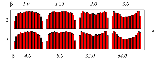
Figure 1: Distribution of the Polyakov line (4), $-1<P<1$, for different $\beta$ and $N_{t}$. Note different $\beta$ range for different $N_{t}$.

A sample of results for different $N_{t}(\equiv N_{D})$ and $\beta$ is shown in Fig. 1. Indeed, for each $N_{t}$, we see a definite change of the shape with $\beta$. This is the first result: the system (2) shows unambigously the onset of the phase change, even in the quenched approximation and for $N=2$.

$N_{t}$	$\beta_{low}$	$\beta_{up}$
2	1.25	1.5
3	3.5	5.0
4	8.0	16.0
5	15.0	40.0
$fit:\;\;\;\;$ $\beta_{c}=\alpha N_{t}^{\gamma}$
$\chi^{2}/NDF$	$\alpha$	$\gamma$
$.55/2$	$.17\pm.05$	$3.02\pm.33$

Table 1: Estimated location of the transition region $\beta_{c}\in(\beta_{low},\beta_{up})$ for different lattice sizes $N_{t}$ and results of the power fit.

Second, the dependence of the pseudocritical temperature $\beta_{c}$ on the time extent $N_{t}$ is consistent with the continuum limit expectations $T_{c}\sim(g^{2}N)^{1/3}$ [13]. Indeed, the temperature of a system is given by $T=1/(aN_{t})$ . Together with (3) these relations imply $\beta_{c}\sim N_{t}^{3}$. The estimates for $\beta$ intervals where the change of phases occur are presented in Table 1 for several lattice sizes $N_{t}$. Results of the power law fit are also quoted. A good quality of the fit and the agreement with the canonical exponent, $\gamma=3$, is encouraging. Simultaneously, we obtain the proportionality coefficient $\alpha$ which translates into

$$T_{c}=({\alpha\over 2N^{2}})^{1/3}(g^{2}N)^{1/3}=(.28\pm.03)(g^{2}N)^{1/3}.$$ (5)

To summarize this point: the observed dependence of $\beta_{c}$ on $N_{t}$ agrees with the canonical scaling expectations for the one dimensional system, and indicates the finite value of the transition temperature in the continuum. Moreover, the coefficient in the continuum relation (5) has been determined for the first time. Only proportionality of the two scales has been considered until now [15, 2, 13]. Since both the pseudocritical temperature and $\alpha$ depend in general on $N$, it is important to repeat similar analysis for higher gauge groups.

Next we study the temperature dependence of the total size of the system $R^{2}=g^{2}\sum_{a}(A_{i}^{a})^{2}$ [13]. We define for $SU(2)$

$$\left\langle{R^{2}}\right\rangle\equiv\left(4-\left\langle{(\mbox{\rm Tr}(U_{s}))^{2}}\right\rangle\right)/a^{2},$$ (6)

where $U_{s}$ is any space link. Due to the periodicity ($N_{s}=1$) in space (6) is gauge invariant. The space links $U_{s}$ are the remnants of the torelon observables well known in lattice QCD [17].

One dimensional Yang-Mills coupling $g$ provides a single scale for all continuum observables similarly to $\Lambda_{QCD}$ in four dimensions. In the following all dimensional quantities quoted in units of $g^{2/3}$ are denoted by a tilde.

Even though the quantum mechanical system (2) is much simpler than the full $D$-dimensional field theory, extracting the continuum limit of the lattice formulation (2) may be a nontrivial task. For example, the above limit contains the complete information about both the perturbative weak coupling and nonperturbative strong coupling regimes in the continuum. Technically, relation (3) implies that a reasonably small lattice constant, $a$ requires simulation with a very large coupling $\beta$. In addition, the one dimensional systems are harder to thermalize. All this poses an interesting challenge in constructing new algorithms suitable for this problem. Some of such alghorithms are under development and will be discussed elsewhere. Here we use mostly the standard local Metropolis update. To overcome the critical slowing down we simply increase the number of thermalization and decorrelation sweeps with $\beta$, until results become independent of the starting configuration. This turned out to be in accord with the dynamical exponent $z=2$. For example when running at $\tilde{a}=1.0$ we used 5000 thermalization and 50 decorrelation sweeps, while for $\tilde{a}=0.1$ about $10^{6}$ thermalization and 5000 decorrelation sweeps were required. One of the new algorithms mentioned above is the SU(2) heat bath designed for an update of the space-space plaquettes in (2) which contain twice the same link. Current version is effective only for $\beta<64$. Results obtained with the new heat bath and the standard Metropolis agree within statistical errors. To check independently the performance of the Metropolis algorithm for higher $\beta$ we have also monitored the correlation length in the torelon channel at zero (i.e. low) temperature. It reveals the expected canonical scaling with $a$.

Fig. 2 shows the dependence of $\tilde{R}^{2}$ on $\tilde{a}$, for several values of the temperature $\tilde{T}$. MC results depend smoothly on $a$, at fixed T, which confirms the existence of the continuum limit (6). The $a$ dependence is clearly different in low and high temperature regions. For $.1<\tilde{T}<.3$, $\left\langle{\tilde{R}^{2}}\right\rangle$ is practically independent of $\tilde{a}$ and points for different (but small) $\tilde{T}$ collapse on the same line. For higher $\tilde{T}$ quadratic minimum at $\tilde{a}=0$ develops and shrinks with the further increase of the temperature. For $\tilde{T}>1.5$ simulations for smaller $\tilde{a}$ are required in order to see this structure and determine the continuum limit. We have also extracted $\left\langle{R^{2}}\right\rangle$ from another lattice observable $|Tr(U_{s})|$ with practically the same results.

Fig. 3 shows the size of a system extrapolated to $a=0$ as a function of the temperature. Both quadratic and quartic fits of $a$ dependence were used to perform the extrapolation [18]. We have also checked the stability of quadratic fits with respect to removing one or two data points with smallest $a$ (highest $\beta$). Results of the extrapolation were stable with respect to all these variations. Small systematic shifts are included in the errors displayed in Fig. 3. The location of the transition region is in rough agreement with the estimate (5) of the pseudocritical temperature $\tilde{T_{c}}=0.35\pm 0.04$ . Again, it is evident that the system is indeed different in the two regimes. Moreover, our results agree qualitatively with the analytical prediction obtained by solving a gap equation in the infinite N limit [13]. The latter gives a temperature independent constant at low temperatures and the classical $T^{1/2}$ growth for high temperatures. We have also found a reasonable agreement with a simple mean field model for $SU(2)$ with the gauge projection. As expected the model does not have a phase transition, but shows a smooth crossover located as in Fig.3. The constant value for $\left\langle{R^{2}}\right\rangle$ is satisfactorily reproduced in the low temperature, vacuum driven region. At higher temperatures the model predicts intermediate linear, albeit weaker than MC, behaviour which asymptotically turns over into $T^{1/2}$ as in the infinite $N$ case.

3. Conclusions. We have constructed the matrix model of M-theory on a lattice in $D$=2,4,6 and 10 dimensions. The resulting system corresponds to the supersymmetric formulation of Yang-Mills theory on the asymmetric $D$-dimensional lattice with all $D-1$ space extensions $N_{s}=1$. The new construction was tested in the quenched approximation for $D$=4. In particular, we have found the onset of a black hole to strings transition even for the $SU(2)$ gauge group. The pseudocritical temperature was determined. The size of the system was also measured at different temperatures and lattice cut-offs. It shows the expected canonical scaling. After extrapolation to the continuum limit it confirms the existence of the two phases and agrees qualitatively with the mean field calculations.

A host of new applications can follow. On the technical side, new algorithms are required to reduce the critical slowing down at very large values of the lattice coupling. Such studies have already begun. Including dynamical fermions is facilitated by the linear nature of the system and may lead to more efficient fermionic algorithms. Certainly the issue of dynamical fermions is very important especially in the low temperature phase since one expects that supersymmetry should be broken only in a minimal fashion there. With dynamical fermions in $D$=10 one may have to use the recently proposed chiral formulation [10]. On the other hand for the reduced system the task may be simpler than e.g. for QCD. It would also be very interesting to apply analytical methods developed in [19, 20]. Incidentally, a merit of the present approach is the possibility to draw from the expertise, techniques and algorithms developed in the lattice community.

A systematic study of the model for higher $N$ would allow finite size analysis and determine more detailed characteristics of the transition. In particular it would be interesting to check if the “soft” dependence on $N$ observed for 3D and 4D $SU(N)$ lattice YM [12], persists in the SYM quantum mechanical model.

Finally, one of the ultimate physical goals would be to study the thermodynamics of the black-hole phase in the full D=10 model and verify existence of the rich phase structure predicted by the string/M theory [2]. This would also provide a possible nontrivial quantitative test of (a version of) the AdS/CFT correspondence at strong coupling not protected by any nonrenormalization theorems [3, 21].

Last but not least, many other problems inspired by the BFSS conjecture can be quantitatively studied.

Acknowledgements. This work is supported by the Polish Committee for Scientific Research under grants no. PB 2P03B00814 and PB 2P03B01917.

Figures

Figure 2: Dependence of the total size of the system on $a$, for $\tilde{T}=.1-.3,.6,.9,1.2$ and $1.5$ (upwards) in units of $g^{2/3}$. Quartic fits are represented by the solid lines.

Figure 3: Size of the system (6) extrapolated to the continuum, as a function of the temperature.

References

- [1] T. Banks, W. Fishler, S. Shenker and L. Susskind, Phys.Rev. D55 (1997) 6189; hep-th/9610043.
- [2] For a recent review see E. J. Martinec, hep-th/9909049.
- [3] For a concrete suggestion see e.g. J. Polchinski, Prog. Theor. Phys. Suppl. 134 (1999) 158; hep-th/9903165.
- [4] H. Aoki et al., hep-th/9908141; N. Ishibashi, S. Iso, H. Kawai and Y. Kitazawa, hep-th/9910004.
- [5] J. Ambjorn, Y. M. Makeenko, J. Nishimura and R.J. Szabo, JHEP 9911:029,1999; hep-th/9911041.
- [6] W. Krauth, H. Nicolai and M. Staudacher, Phys. Lett.B431 (1998) 31; hep-th/9803117, Phys. Lett. B435 (1998) 350; hep-th/9804199; G. Moore, N. Nekrasov and S. Shatashvili, Commun. Math. Phys. 209 (2000) 77; hep-th/9803265.
- [7] U. H. Danielsson, G. Ferrati and B. Sundborg, Int. J. Mod. Phys. A11 (1996) 5463; hep-th/9603081.
- [8] L. Brink, J. H. Schwarz and J. Scherk, Nucl. Phys. B121 (1977) 77.
- [9] I. Campos et al., Eur. Phys. J. C11 (1999) 507; hep-lat/9903014.
- [10] M. Lüscher, hep-lat/9909150 and references therein.
- [11] D. Weingarten, Phys. Lett. B109 (1982) 57; H. Hamber and G. Parisi, Phys. Rev. Lett. 47 (1981) 1792;
- [12] M. Teper, Phys. Lett. B397 (1997) 223, hep-lat/9711011; Phys.Rev. D59 (1999) 014512; hep-lat/9804008.
- [13] D. Kabat and G. Lifszytz, hep-th/9910001.
- [14] A. Strominger and C. Vafa, Phys. Lett. B379 (1996) 99.
- [15] G.T. Horowitz and J. Polchinski, Phys.Rev. D55 (1997) 6189, hep-th/9612146.
- [16] D. J. Gross and E. Witten, Phys. Rev. D21 (1980) 446.
- [17] C. Michael, Nucl. Phys. B329 (1991) 225.
- [18] K. Symanzik, Nucl. Phys. B226 (1983) 187.
- [19] M. Lüscher, Nucl. Phys. B219 (1983) 233.
- [20] P. van Baal, Acta Phys. Polon. B20 (1989) 295.
- [21] T. Yoneya, hep-th/9908153.