DFTT 8/2000

February 2000

Lattice Gauge Theories and the

AdS/CFT Correspondence.

M. Caselle

Istituto Nazionale di Fisica Nucleare, Sezione di Torino

Dipartimento di Fisica Teorica dell’Università di Torino

via P.Giuria 1, I-10125 Turin,Italy

This is the write-up of a set of lectures on the comparison between Lattice Gauge Theories and AdS/CFT results for the non-perturbative behaviour of non-supersymmetric Yang Mills theories. These notes are intended for students which are assumed not to be experts in L.G.T. For this reason the first part is devoted to a pedagogical introduction to the Lattice regularization of QCD. In the second part we discuss some basic features of the AdS/CFT correspondence and compare the results obtained in the non-supersymmetric limit with those obtained on the Lattice. We discuss in particular the behaviour of the string tension and of the glueball spectrum. Lectures delivered at the School of Theoretical Physics  (S.N.F.T.),  Parma,  September 1999.

1 Introduction

Our present understanding of QCD is based on the widely accepted idea that the confining regime of Yang-Mills theories should be described by some kind of effective string model [1, 2].

This conjecture has by now a very long history. It originates from two independent observations.

• The first one is of phenomenological nature, and predates the formulation of QCD. It is related to the observation that the linearly rising Regge trajectories in meson spectroscopy can be easily explained assuming a string-type interaction between the quark and the antiquark. This observation was at the origin of a large amount of papers which tried to give a consistent quantum description of strings.

• The second one comes from the lattice regularization of pure gauge theories (LGT in the following) and was realized right after the formulation of QCD. In the LGT framework one can easily study non-perturbative phenomena, like those involved in the conjectured string description of $YM$ theories and it is easy to see that in the strong coupling limit of pure LGTs the interquark potential rises linearly, and that the chromoelectric flux lines are confined in a thin “string like” flux tube [3].

Some clear indications were later found that the vacuum expectation value of Wilson loops could be rewritten as a string functional integral even in the continuum [4, 5, 6]. This led to conjecture that there exists an exact duality between gauge fields and strings [4].

However, despite these results, in the following years all the attempts to explicitly construct the conjectured string description of QCD failed. In fact it was realized at the beginning of the eighties that the strong coupling approximation for the lattice description of interquark potential is plagued by lattice artifacts which make it inadequate for the continuum theory (this is the famous “roughening transition” that we shall discuss in sect. 3.5.1).

Since then, while impressive results were obtained by means of Montecarlo simulations, very little progress have been achieved with analytic techniques. Lattice gauge theories can be solved exactly in two dimensions for any gauge group, but become unaffordably complex in more than two dimensions, even in absence of quarks. Moreover, most of the approximation techniques which are usually successful in dealing with simpler statistical mechanical systems, like (suitably improved) mean field methods or strong coupling expansions turn out to be less useful in the case of LGT.

Several proposals were made during the eighties to overcome these difficulties. In particular, two of them led to rather interesting results.

Effective string theory

The first proposal was to assume a milder version of the conjecture. This milder version only requires that the behavior of large Wilson loops is described in the infrared limit by an effective two-dimensional field theory (hence not a true string theory) which accounts for the string-like properties of long chromoelectric flux tubes. We shall refer to such a $2d$ field theory in the following as the “effective string theory”. Several interesting results can be obtained in this framework. We shall discuss them in detail in sect. 3.5 below. Let us anticipate here that the most interesting feature of this approach is that it leads to predictions which are in very good agreement with the results of Montecarlo simulations of QCD. Its major drawback is that it is not consistent at the quantum level. It is not clear how to extend this effective string description to the ultraviolet regime, i.e. how to relate it with some kind of “fundamental” string which is consistent at the quantum level.

Large $N$ limit

The second proposal was to study the large $N$ limit of $SU(N)$ gauge theories instead of the phenomenologically relevant $SU(3)$ model [2]. It was shown that this large $N$ approximation [7] is able to keep the whole complexity of the finite $N$ models. Unfortunately, even in the large $N$ limit (despite the fact that some major simplifications occur) it is not possible to give exact solution (the so called “Master Field”) to the Lattice SU$(N)$ model and essentially no improvement was made in these last fifteen years also in this direction.

Recently this situation drastically changed thanks to a new, original proposal based on the Maldacena conjecture [8] which relates the large $N$ expansion of certain supersymmetric gauge theories to the behaviour of string theory in a non-trivial geometry. Witten’s extension [9] of this conjecture to non-supersymmetric gauge theories, led to the hope of a possible non-perturbative description also for large $N$ QCD in four dimensions. In fact in these last months several attempts have been made to extract predictions for the string tension and the glueball spectrum of large $N$ QCD. These predictions have some appealing features, but also raised serious criticism. All the authors agree that some independent test of the applicability of the AdS/CFT correspondence to large $N$ QCD is needed. This is indeed possible thanks to the impressive progress of montecarlo simulations of LGT which have by now reached stable estimates both of string tension and glueball spectrum for finite $N$ and allow reliable extrapolations to the large $N$ limit.

The aim of these lectures is to allow the reader (which is assumed $not$ to be an expert of LGT) to understand how these estimates were obtained and to test their reliability. We shall also compare the “effective string model” mentioned above with the string theory which is at the basis of AdS/CFT model. The goal is to be able not only to accept or reject the AdS/CFT predictions on the basis of the LGT results but also, if possible, to gain some insight in the AdS/CFT proposal itself.

To this end we shall devote the first part of these lectures (sect. 2 and the first part of sect. 3) to an elementary introduction to the lattice regularization of QCD, starting form the very beginning. Then in the second part of the lectures (from sect. 3.4 to 3.7) we shall jump to our main object of interest and study in some detail the LGT results for the string tension and the glueball spectrum.

Unfortunately we shall have to skip several important and interesting hot topics of LGT, like the issue of improved (and “perfect”) actions, that of chiral fermions, topological observables, deconfinement transition …. We leave the interested reader to the books and review articles listed at the end of the bibliography [73]-[86] (we tried to make the list as complete as possible) which summarize the present state of the art in LGT.

The last part of these lectures (sect.s 4 and 5) is devoted to the AdS/CFT correspondence and in particular to discuss its predictions for the non-perturbative behaviour of non-supersymmetric Yang-Mills theories. Let us stress in this respect that this set of lectures is not intended as an introduction to the AdS/CFT correspondence for which we refer to the other lectures delivered at this school and to two thorough reviews which already exist on the subject [87],[88]. In this lectures we shall assume that the reader is already acquainted with the topic and shall only remind some basic informations at the beginning of sect. 4.

2 Introduction to Lattice Gauge Theories.

2.1 Quantum Field Theories and Statistical Mechanics.

The modern approach to Quantum Field Theories (QFT in the following) is based on Feynman’s path integral formulation. Using path integrals impressive results have been obtained in the last fifty years in perturbative QFT However these methods require the existence of one (or more) weak coupling parameters in which the theory can be expanded perturbatively. As such they are not suited for the analysis of phenomena governed by intrinsically large coupling constants, or even worse, with a non-analytic behaviour at the origin, in the space of complex coupling parameters. This is exactly the case of QCD, at least as far as dimensional observables are concerned. To overcome these difficulties a different regularization was proposed almost thirty years ago by K. Wilson [3]. Wilson suggested to formulate the theory on a discrete lattice of points in Euclidean space-time. Such proposal has some very important advantages:

• The path integral becomes a collection of well defined ordinary integrals at the lattice sites.

• The lattice spacing becomes an ultraviolet cut-off.

• As far as the number of sites of the lattice is kept finite all the ultraviolet divergences are removed and all quantum averages are given by mathematically well defined expressions, for any value of the coupling constant.

• A QFT in $d$ space and 1 time dimensions regularized on a lattice becomes equivalent to an equilibrium statistical mechanics model in $(d+1)$ space dimensions. As a consequence one can study the model with all the tools which are typical of statistical mechanics like strong coupling expansion or Montecarlo simulations.

Obviously the lattice regularization is not a magic wand and all the problems which have been overcome appear again, in some other form, when we take the continuum limit (we shall deal with this very delicate issue in sect. 2.3). However the main feature of the regularization, i.e. the fact that it is intrinsically non-perturbative survives in the limit and allows one to obtain results which could never be obtained with standard perturbative expansions .

In this section we shall discuss in details the two main steps which allow one to construct (and extract results from) a lattice regularization of QFT:

a] The translation from Minkowski to Euclidean Quantum Field Theory

b] The connection between Euclidean QFT and Statistical Mechanics in the canonical Ensemble.

The starting point for a path integral formulation of QFT is the vacuum to vacuum amplitude (also called the generating functional) in presence of an external source $J$

$$Z[J]=\int d\phi e^{\frac{i}{\hbar}\int dt\int d^{3}x{\cal L}(\phi)+J\phi}~{}~{}~{}~{}.$$ (1)

Correlation functions can be obtained from this in the standard way by differentiating $\log Z[J]$ with respect to $J$, for example

$${\big{\langle}0\big{|}T[\phi(x)\phi(0)]\big{|}0\big{\rangle}}={\delta\over\delta J(x)}{\delta\over\delta J(0)}\log Z[J]|_{J=0}~{}~{}~{}.$$ (2)

Looking at eq.(1) we immediately recognize the analogy with the usual expression of the partition function in the canonical ensemble. The only difference (which is however of great importance) is that in the exponential of eq.(1) we have an oscillatory term while the argument in the exponent of a Boltzmann weight is real. We can bridge this difference with an analytic continuation of eq.(1) to imaginary values of the time. This is the well known “Wick rotation”.

$$x_{0} \equiv t\to-ix_{4}\equiv-i\tau\,,$$

$$p_{0} \equiv E\to ip_{4}\,.$$ (3)

In this way we obtain

$$Z[J]=\int d\phi e^{-{\cal S}_{E}+J\phi}$$ (4)

where ${\cal S}_{E}$ denotes the Euclidean action. We shall discuss in detail its form in the Yang Mills case in the next section. At this point we may well interpret ${\cal S}_{E}$ as the Hamiltonian of a static model in four space dimensions and $Z[J]$ with the corresponding partition function. It is far from obvious that we can perform a Wick rotation without problems. On the continuum this is granted by the good analyticity properties of the propagator, but on the lattice it imposes some strict constraint on the form of the discretized action. These constraints are known as reflection positivity conditions [10] (and also as “Osterwalder and Schrader positivity conditions”).

The connection between QFT and Statistical mechanics is a crucial issue of modern quantum field theory. It has deep, far reaching, consequences in several physical contexts. Its main implications are summarized in tab. 1

Table 1: The equivalence between a Euclidean field theory and Classical Statistical Mechanics.

Euclidean Field Theory	Classical Statistical Mechanics
Vacuum	Equilibrium state
Action	Hamiltonian
unit of action $h$	units of energy $\beta=1/kT$
Feynman weight for amplitudes	Boltzmann factor $e^{-\beta H}$
$\qquad e^{-{\cal S}/h}=e^{-\int{\cal L}dt/h}$
Generating functional	Partition function $\sum_{conf.}e^{-\beta H}$
$\int{\cal D}\phi e^{-{\cal S}/h}$
Vacuum energy	Free Energy
Vacuum expectation value ${\big{\langle}0\big{|}{\cal O}\big{|}0\big{\rangle}}$	Canonical ensemble average ${\big{\langle}{\cal O}\big{\rangle}}$
Time ordered products	Ordinary products
Green’s functions ${\big{\langle}0\big{|}T[{\cal O}_{1}\ldots{\cal O}_{n}]\big{|}0\big{\rangle}}$	Correlation functions ${\big{\langle}{\cal O}_{1}\ldots{\cal O}_{n}\big{\rangle}}$
Mass $M$	correlation length $\xi=1/M$
Mass-gap	exponential decrease of correlation functions
Mass-less excitations	spin waves
Regularization: cutoff $\Lambda$	lattice spacing $a$
Renormalization: $\Lambda\to\infty$	continuum limit $a\to 0$
Changes in the vacuum	phase transitions

2.2 Lattice discretization of pure Yang-Mills theories

The goal of this section is the explicit construction of a lattice regularization of a gauge theory with gauge group ${\bf G}$. To this end we need first of all a Wick rotated, Euclidean formulation of the theory (sect. 2.2.1). Then for its lattice discretization three main ingredients are needed: the lattice structure (sect. 2.2.2), the lattice definition of the gauge variables (sect. 2.2.3) and the action (sect. 2.2.4). In each of these steps we have a great amount of freedom. We shall always choose the simplest option, and leave to exercise 1 the discussion of possible alternative choices. We shall then check in sect. 2.2.5 that the proposed action gives in the “naive” continuum limit the expected gauge invariant expression and add some further remarks on the integration measure (sect. 2.2.6), on the fermionic sector (sect. 2.2.7) and on the constraints which must be imposed to obtain a finite temperature version of the theory (sect. 2.2.8).

2.2.1 Euclidean Yang-Mills theories

In the following we shall be interested in the lattice formulation of $YM$ theories. The continuum limit of these models is the Euclidean version of $YM$ theories. Let us briefly remind its expression. The building blocks are the field $A_{\mu}^{i}$, $i=1...N$ where $N$ is the number of the generators of the gauge group. The indices $i,j,...$ run in the space of the generators of the gauge group. The Yang Mills action is:

$$S_{YM}=\frac{1}{4}\int d^{4}xF_{\mu\nu}^{i}F^{i~{}\mu\nu}$$ (5)

with

$$F_{\mu\nu}^{i}=\partial_{\mu}A_{\nu}^{i}-\partial_{\nu}A_{\mu}^{i}+gf_{ijk}A^{j}_{\mu}A^{k}_{\nu}$$ (6)

where $g$ is the coupling constant and $f_{ijk}$ are the structure constants of the gauge group defined by

$$[\tau_{i},\tau_{j}]=if_{ijk}\tau_{k}~{}~{}~{}.$$ (7)

2.2.2 The lattice

Let us choose the simplest possible lattice structure: a four dimensional hypercubic lattice ${\bf\Lambda}$ of size $L$ in the four directions. Let us denote the sites of the lattice with $n\equiv(n_{0},n_{1},n_{2},n_{3})$ and with $\hat{\mu}$ the unit vector in the $\mu$ direction $(\mu=0,1,2,3)$. We shall often call in the following the $0$ direction as time-like and the other three as space-like, but let us stress that, due to the Wick rotation, all four directions are exactly on the same ground (we shall make use of this symmetry in the following). ${\bf\Lambda}$ contains $N_{s}~{}=~{}L^{4}$ sites, $N_{l}~{}=~{}4~{}L^{4}$ links and $N_{p}~{}=~{}6~{}L^{4}$ plaquettes. We shall denote with $n_{\mu}$ the link starting form $n$ and pointing in the positive $\mu$ direction i.e the link joining the two sites $n$ and $n+\hat{\mu}$. Similarly $n_{\mu,\nu}$ denotes the plaquette joining the four sites $n$, $n+\hat{\mu}$, $n+\hat{\mu}+\hat{\nu}$, $n+\hat{\nu}$. We shall denote with $a$ in the following the “lattice spacing” i.e. the separation between two nearby sites.

2.2.3 The gauge field.

There is a standard recipe to choose the lattice analog of the bosonic fields of a continuum QFT. One must define the scalars on the sites, the vectors on the links and the two index tensors on the plaquettes of the lattice. This recipe can be simply understood if we rewrite the QFT in terms of differential forms. The discrete analog of a p-form is a p-simplex. In whole generality this rule can be stated as follows:

“The lattice analog of a tensor field of degree $k$ is a function which takes values on the $k$ simplexes of the lattice”

Thus the vector potential $A_{\mu}(x)$ must be defined on the links of the lattice. The simplest choice, which ensures both gauge invariance and a smooth continuum limit is to put in each link $n_{\mu}$ an element of the gauge group: $U_{\mu}(n)\in{\bf G}$ such that

$$U_{\mu}(n)=e^{cA_{\mu}(n)}$$ (8)

where $c$ is a suitable constant which we shall discuss below.

A nice, intuitive, way to understand this choice is the following: Imagine that in each site $n$ does exist an internal space $E$ (on which the gauge group $\bf G$ acts in a non trivial way). Let us assume that the reference frame $E_{n}$ on $E$ changes from site to site. Then we can interpret $U_{\mu}(n)$ as the transformation which relates the two nearby reference frames $E_{n}$ and $E_{n+\hat{\mu}}$. An immediate consequence of this picture is that we must impose, for consistency:

$$U_{-\mu}(n+\hat{\mu})=U_{\mu}^{-1}(n)$$ (9)

In this framework a gauge transform is simply an arbitrary rotation, site by site of the reference frames $E_{n}$. Let us denote these transformations as $V(n)\in{\bf G}$. It is clear that the effect on $U_{\mu}(n)$ of such transformations is the following

$$U_{\mu}(n)~{}~{}\to~{}~{}V(n)~{}U_{\mu}(n)~{}V^{-1}(n+\hat{\mu})$$ (10)

Thus, as expected, the single variable $U_{\mu}(n)$ is not gauge invariant. The simplest way to construct, out of the gauge variables $U_{\mu}(n)$, gauge invariant observables, is to choose a closed path $\gamma$ on the lattice and then construct

$$W(\gamma)={\rm Tr}\prod_{n_{\mu}\in\gamma}U_{\mu}(n)$$ (11)

(where the product is assumed to be ordered along the path $\gamma$). This observable is usually called “Wilson loop”.

2.2.4 The action

Obviously, the main requirement that we must impose on the discretized version of the action is that it must be gauge invariant. Among all the possible Wilson loops the simplest one is the product of the four link variables around a plaquette. If we sum these elementary Wilson loops over all the plaquettes of the lattice we obtain an expression which is invariant with respect to the discrete subgroups of the translational and rotational symmetries which survive in the lattice discretization. This was the original Wilson proposal for the lattice discretization of the gauge invariant action. Such an expression defines a perfectly consistent gauge invariant model for any group $\bf G$ on the lattice and is a good candidate to define a translational and rotational invariant gauge theory also in the continuum limit. At this stage we have no constraint on $\bf G$ which can well be a finite, discrete group. For instance several interesting results have been obtained in the case in which ${\bf G}=Z_{2}$ (the “gauge Ising model”). However since we are interested in constructing the lattice version of Yang-Mills theories we must concentrate on the case in which $\bf G$ is continuous Lie group. Even if the physically interesting case is ${\bf G}=SU(3)$, we shall study in the following the general case ${\bf G}=SU(N)$ with $N\geq 2$. This extension essentially does not add any further complication and allows to study the limit $N\to\infty$ which is essential if we aim to compare our lattice results with the AdS/CFT predictions.

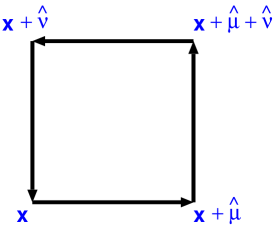
Figure 1: The Wilson action.

Let us see it in detail. Let us define with $U_{\mu\nu}(n)$ the product of the four link variables around the plaquette $n_{\mu\nu}$ (see fig. 1)

$$U_{\mu\nu}(n)=\left\{U_{\mu}(n)U_{\nu}(n+\hat{\mu})U_{-\mu}(n+\hat{\mu}+\hat{\nu})U_{-\nu}(n+\hat{\nu})\right\}$$ (12)

The Wilson action is

$$S_{W}=-\frac{\beta}{2N}\sum_{n,\mu\nu}{\rm Re~{}Tr}\left\{U_{\mu\nu}(n)\right\}~{}~{}~{}~{},$$ (13)

where we have introduced the $\frac{\beta}{2N}$ constant in front of the action for future convenience. Notice that since the sum over $\mu$ and $\nu$ is unrestricted all the plaquettes of the lattice are counted twice. We shall check in the next section that this proposal indeed gives in the continuum limit the correct gauge invariant action.

• Exercise 1: discuss some possible generalizations of the lattice discretization of $SU(N)$ $YM$ theories. In the above derivation we chose at each step the simplest possible option. However there are infinitely many different lattice regularizations which lead to the same continuum limit of eq.(25). Discuss some of these possible generalizations.

2.2.5 “Naive” continuum limit.

Let us call ${\cal G}$ the Lie algebra associated with $\bf G$. Let us assume that ${\cal G}$ has $N$ generators $\tau_{1}\cdots\tau_{N}$. Then we can define:

$$U_{\mu}(n)\equiv e^{iB_{\mu}(n)}$$ (14)

with

$$B_{\mu}(n)\equiv ag\tau_{i}A_{\mu}^{i}(n)$$ (15)

$a$ being the lattice spacing and $g$ a suitable coupling constant. As we shall see the $A_{\mu}^{i}$ functions will become in the continuum limit the standard vector potential fields of the Yang Mills theory.

We may expand the fields appearing in the Wilson action (keeping only the first order in $a$) as follows.

$$B_{\nu}(n+\hat{\mu}) \sim B_{\nu}(n)+a\nabla_{\mu}B_{\nu}(n)$$

$$B_{-\mu}(n+\hat{\mu}+\hat{\nu}) \equiv -B_{\mu}(n+\hat{\nu})~{}~{}\sim~{}~{}-B_{\mu}(n)-a\nabla_{\nu}B_{\mu}(n)$$

$$B_{-\nu}(n+\hat{\nu}) \equiv -B_{\nu}(n)$$ (16)

where we have denoted with

$$\nabla_{\nu}f(n)\equiv\frac{f(n+\hat{\nu})-f(n)}{a}$$ (17)

the finite difference on the lattice, whose continuum limit is the partial derivative:

$$\nabla_{\nu}f(n)~{}~{}\to~{}~{}\partial_{\nu}f(x)~{}~{}~{}~{}~{}.$$ (18)

From the above expansions we obtain:

$$U_{\mu\nu}(n)~{}~{}\sim~{}~{}e^{iB_{\mu}(n)}e^{i(B_{\nu}(n)+a\nabla_{\mu}B_{\nu}(n))}e^{-i(B_{\mu}(n)+a\nabla_{\nu}B_{\mu}(n))}e^{-iB_{\nu}(n)}$$ (19)

Let us use at this point the Baker-Hausdorff formula, which at the first order is:

$$e^{x}e^{y}=e^{x+y+\frac{1}{2}[x,y]}$$ (20)

Keeping in the expansion only terms up to $O(a^{2})$ (remember that $B_{\mu}$ is of order $a$) we find

$$U_{\mu\nu}~{}~{}\sim~{}~{}e^{\left\{ia(\nabla_{\mu}B_{\nu}-\nabla_{\nu}B_{\mu})-[B_{\mu},B\nu]\right\}}\equiv e^{ia^{2}gF_{\mu\nu}}$$ (21)

where we have neglected for simplicity the argument $n$ and we have defined:

$$F_{\mu\nu}\equiv\nabla_{\mu}A_{\nu}-\nabla_{\nu}A_{\mu}+ig[A_{\mu},A_{\nu}]$$ (22)

and $A_{\mu}\equiv\tau_{i}A^{i}_{\mu}$.

Let us insert this result in eq.(13), and expand in powers of $a$. we find:

$$S_{W}\sim-\frac{\beta}{2N}\sum_{n,\mu\nu}{\rm Re~{}~{}Tr}\left({\bf 1}+ia^{2}gF_{\mu\nu}-\frac{1}{2}a^{4}g^{2}F^{2}_{\mu\nu}\right)$$ (23)

We can always parameterize the $SU(N)$ generators so as to have

$${\rm Tr}(\tau_{i})=0,~{}~{}~{}~{}~{}~{}~{}~{}~{}~{}{\rm Tr}(\tau_{i}\tau_{j})=\frac{1}{2}\delta_{ij}~{}~{}~{}~{}.$$ (24)

while ${\rm Tr}~{}{\bf 1}$ only gives an irrelevant constant which can be neglected. In this way we obtain

$$S_{W}=\frac{\beta a^{4}g^{2}}{8N}\sum_{n,\mu\nu}F^{i}_{\mu\nu}F^{i~{}\mu\nu}+O(a^{5})$$ (25)

In the naive limit $a\to 0$ we can set $\sum_{n}\to\int\frac{d^{4}x}{a^{4}}$ (for a four-dimensional lattice) and we see that the dominant term in the $a\to 0$ limit becomes the standard expression of the pure $YM$ action if we set

$$\beta=\frac{2N}{g^{2}}$$ (26)

From this position we see that $\beta$ is proportional to the inverse of $g^{2}$. It is also easy to see, from dimensional arguments that in four dimensions the coupling constant $g$ is adimensional while for 3d $YM$ theories $g^{2}$ has the dimensions of a mass.

2.2.6 The partition function.

As mentioned above, our real interest is not in the gauge action but in the partition function (or generating functional in the QFT language) $Z$. In constructing $Z$ we must address the problem of the integration measure (and the related problem of gauge fixing this integration). Here we see one of the most interesting advantages of the lattice regularization. The integrals involved in the construction of $Z$ are site by site (or better, in the case of a gauge theory, link by link) ordinary integrals. We have a natural choice for the integration measure: the Haar measure (i.e. the invariant measure over the group manifold $dU_{\mu}(n)$). We have:

$$Z=\int\prod_{n,\mu}dU_{\mu}(n)e^{-S_{W}}$$ (27)

and similarly, for a generic expectation value we have

$$\langle{\cal O}\rangle=\frac{\int\prod_{n,\mu}dU_{\mu}(n){\cal O}(U_{\mu}(n))e^{-S_{W}}}{Z}$$ (28)

A remarkable consequence of these definitions is that, since the integration is made, link by link, over the whole group manifold all the gauge equivalent configurations (see eq.(10)) are automatically included in the sum with the correct weight. Contrary to the continuum case, on the lattice, the integration over the pure gauge degrees of freedom does not make quantum averages ill defined. In the lattice regularization there is no need to fix the gauge: all the quantum averages are by construction gauge invariant.

2.2.7 Fermions.

In the previous sections we studied the lattice discretization of pure $YM$ theories. In full QCD we should also take into account the quarks. However putting fermions on the lattice is a rather non trivial issue. Moreover, once a consistent discretization of the theory is obtained if we try to integrate out the fermions from the Lagrangian we obtain a determinant of the gauge fields which is very difficult to handle in Montecarlo simulations. In view of this consideration it has become a common habit to organize lattice gauge theories in three levels of increasing complexity.

• In the first level we find pure $YM$ theories. These models are by now rather well understood and precise Montecarlo results exist for the continuum limit of several quantities, among these the most interesting ones are the glueballs since we may rather safely expect that their mass should not be too affected by the absence of quarks.

• The second level is the so called “quenched QCD” in which the quarks are explicitly added into the game, thus giving the possibility to explore several new observables (for instance the meson spectrum) which are of great interest for the phenomenology, but they are kept quenched, i.e. the determinant mentioned above is simply neglected. This means that in the partition function the quarks are treated as classical quantities or equivalently that we are neglecting quark loops in our calculations. Also for quenched QCD stable and reliable result have been obtained from Montecarlo simulations. However there are effects, like the string breaking at large distance, which are a typical consequence of quarks loops and that cannot be observed in the quenched approximation. Moreover it is by now clear that several quantities of great physical interest (like the meson spectrum or the temperature of the chiral phase transition) are heavily affected by such approximation.

• The third level is that in which full QCD, with dynamical fermions is discretized on the lattice. In this last case Montecarlo simulations are still at a preliminary stage and a few years (and the next generation of supercomputers) will be needed before we may reach stable and reliable results also in this case.

Luckily enough, the predictions of the AdS/CFT correspondence, whose comparison with the lattice results is the main goal of these lectures, refer to the pure $YM$ theories. Thus on the lattice side of the comparison we may rely on very stable and trustable numbers. Moreover in pure $YM$ theories extensive simulations exist in three dimensions also for values of $N$ larger than 3 and reliable large $N$ limits for various quantities of interest can be obtained [83]. In four dimensions the results of these large $N$ limits are still preliminary [84], but nevertheless they are stable enough to allow for the comparison with the AdS/CFT results. In the following, both in the lattice sections and in the AdS/CFT ones we shall make an effort to keep well distinct those results which refer to pure Yang Mills theories from those which refer to full QCD.

2.2.8 Finite temperature LGT.

We shall see in sect. 4 that in the framework of the AdS/CFT correspondence a very important role is played by the “temperature” of the theory. It turns out that it is only at high temperature that we can get rid of the supersymmetry and obtain non-supersymmetric Yang-Mills like theories. It is thus important to understand how can we describe finite temperature on the lattice.

The model that we have defined and studied in the previous sections describes $YM$ theories at strictly zero physical temperature. The parameter which in the statistical mechanics counterpart of the model plays the role of the temperature becomes in LGT the coupling constant of theory. The discussion of sect. 2.1 can be easily extended so as to implement a non-zero temperature also in LGT. The main ingredient is that periodic boundary conditions must be imposed in the “time direction”. Then it can be shown that the inverse of the lattice size in this direction is proportional to the temperature of the theory.

In general, for technical reason, one imposes periodic boundary conditions in all the $d$ directions, but one also takes care to choose the lattice length much larger that the typical correlation length of the theory, so as to make negligible the effect of the boundary conditions. On the contrary if we want to see the effects of the finite temperature in the theory, the lattice size in the “time” direction must be chosen of the same order of the correlation length. If we increase the lattice size in the “time” direction then we smoothly reach the zero temperature limit, which is effectively reached when the effects of the periodic boundary condition become negligible. Thus typically a finite temperature discretization requires asymmetric lattices, with one direction much shorter than the others. As a consequence the original equivalence of space and time directions which is a typical feature of Euclidean QFT is lost. In finite temperature LGT (FTLGT in the following), we have a very precise notion of “time” which is the compactified direction proportional to the inverse of the temperature.

Due to the presence of periodic boundary conditions a new class of observables exists in FTLGT i.e. the loops which close winding around the compactified time direction. These are usually called Polyakov loops. The discussion of FTLGT (apart from a few issues that we shall address in sect. 3) is beyond the scope of these lectures. We refer to the reviews in the bibliography for further details.

2.3 Continuum limit

It is clear that by simply sending $a\to 0$ as in the previous section we do not obtain a meaningful continuum limit. In particular, all the dimensional quantities, which will be proportional to a non-zero power of $a$ will go to zero or infinity. This is the meaning of the word “naive” used above.

Let us study this problem in more detail. Let us take a physical observable ${\cal O}$ of dimensions $d_{\cal O}$ in units of the lattice spacing. Let us assume that we have in some way calculated the mean value of ${\cal O}$ in the lattice regularized version of the theory. The result of this calculation will take the form:

$$\langle{\cal O}\rangle=a^{d_{\cal O}}f_{\cal O}(g)$$ (29)

where $f_{\cal O}(g)$ is a suitable function of the coupling constant of the theory (in general of all the parameters of the model if they are more than one). For instance ${\cal O}$ could be one of the correlation lengths of the model (i.e. the inverse of the mass of one of the states of the theory). In this case $d_{\cal O}=1$ and $f_{\cal O}(g)$ measures the correlation length in units of the lattice spacing, for the particular value $g$ of the coupling constant. It is now clear that if we simply send $a\to 0$ we obtain the trivial result $\langle{\cal O}\rangle=0$. In order to have a meaningful continuum limit we must change $g$ at the same time as $a$ is set to zero in such a way as to make the observable to approach a well defined finite value in the limit. In the example this means that we must tune $g$ to a critical value $g_{c}$ in which the correlation length measured in units of the lattice spacing goes to infinity.

From a statistical mechanics point of view this implies that at $g=g_{c}$ the system must undergoes a continuous phase transition. This is a mandatory requirement for a non-trivial continuum limit. From the point of view of QFT we have a nice interpretation of this constraint. While the lattice discretization gives a way to regularize the theory. The process of tuning $g$ to its critical value, thus removing the cut-off, corresponds to the renormalization of the theory.

This process is highly non trivial, since for all the physical quantities ${\cal O}_{i}$ that we may define in the model we must require a well defined continuum limit. If $f_{i}(g)$ is the function which measures the value of ${\cal O}_{i}$ in units of the lattice spacing, then we must require that as $g\to g_{c}$ all the functions $f_{i}(g)$ go to zero or infinity (depending on the sign of $d_{{\cal O}_{i}}$) in such a way that the same rate of approach of $g$ to $g_{c}$ which makes the correlation length $\xi$ tend to a constant value also makes all the observables ${\cal O}_{i}$ tend to constant values. This stringent requirement is better understood in the framework of the Renormalization Group approach and is commonly summarized, by saying that the critical point $g_{c}$ must be a scaling critical point.

It is clear from the above discussion that a meaningful continuum limit requires a precise functional relationship between $a$ and $g$. However in principle we can even ignore such a dependence. The notion of scaling defined above allows to reach a well defined continuum limit even if we do not know how to fix $g$ as a function of $a$. If we know the physical value of one of the observables of the theory, say the mass $m_{e}$ of a particle “e” which is easily accessible from the experiments, then we may set the overall scale of the theory as follows

$$m_{e}=\frac{1}{a(g)\xi_{e}(g)}$$ (30)

where $\xi_{e}(g)$ is the particular correlation length related to the particle “e”. Then the continuum limit value of any other dimensional quantity of the theory, like for instance the masses $m_{i}$ of other particles, can be obtained as

$$m_{i}=\lim_{a\to 0}\frac{1}{a(g)\xi_{i}(g)}~{}=~{}\lim_{g\to g_{c}}\frac{\xi_{e}(g)}{\xi_{i}(g)}m_{e}$$ (31)

This is the power of scaling!

In some cases it may happen that, on top of the above relations, we also have some independent way to fix asymptotically (i.e. in the vicinity of the critical point) the relationship between $g$ and $a$. This is the exactly the case for non-abelian gauge theories, for which asymptotic freedom tells us that $g_{c}=0$ and perturbative methods can be used. This leads to the following well known expression, for a pure $SU(N)$ gauge theory in four dimensions:

$$a=\frac{1}{\Lambda}f(g)$$ (32)

with

$$f(g)=(g^{2}\beta_{0})^{\beta_{1}/(2\beta_{0})}e^{-1/(2\beta_{0}g^{2})}(1+O(g^{2}))$$ (33)

where

$$\beta_{0}=\frac{11N}{48\pi^{2}},~{}~{}~{}\beta_{1}=\frac{34}{3}\left[\frac{N}{16\pi^{2}}\right]^{2}$$ (34)

are the first two coefficients of the Callan-Symanzik function $\beta(g)$ and $\Lambda$ is a scale parameter, which does not have a direct physical meaning and in general depends on the renormalization scheme that we have chosen (for instance it may depend on the type of lattice that we have chosen).

One usually refers to this relation (and to the procedure of taking the continuum limit following eq.(33)) as “asymptotic scaling” to stress the fact that one is using more informations than those simply implied by the scaling property.

Since it will play an important role in the following it is worthwhile to discuss in detail how one should use eq.(33). To this end let us continue with the above example, and let us assume again that ${\cal O}$ is the correlation length of the theory (i.e the inverse of the lowest glueball). Let us measure it on the lattice for various values of $g$ in the scaling region in units of the lattice spacing $a$ and let us call these numbers (which at this point are pure adimensional numbers) $\xi(g)$. We have

$${\cal O}=a\xi(g)$$ (35)

Let us now insert eq.(32), we find

$${\cal O}=\frac{f(g)\xi(g)}{\Lambda}$$ (36)

Our goal is to find a finite continuum limit value (let us call it $\frac{\xi_{0}}{\Lambda}$) for ${\cal O}$. This implies that $\xi(g)$ must scale as:

$$\xi(g)=\frac{\xi_{0}}{f(g)}$$ (37)

If this condition is fulfilled by the data then we may say that the lowest glueball has a mass in the continuum limit whose values is

$$m=\frac{1}{\xi}_{0}\Lambda$$ (38)

if we are able to fix the value of $\Lambda$ in $MeV$ (and this can be done, for instance, by comparing the string tension evaluated on the lattice with the physical value of the string tension obtained from the spectroscopy of the heavy quarkonia) then eq.(38) will give us the value in $MeV$ of the lowest glueball. The precision of this prediction will only be limited by the uncertainty in the determination of $\Lambda$ in $MeV$ and by the statistical and systematic errors which affect the estimate of the amplitude $\xi_{0}$ from a fit to the data $\xi(g)$ according to eq.(37).

Let us conclude this section by noticing that the functional dependence on $g$ of eq.s(32),(33) is a direct consequence of the fact that the coupling $g^{2}$ in this case is adimensional. In fact the scaling behaviour for $SU(N)$ gauge theories in three dimensions is completely different. In this case it is $g^{2}$ itself (which has the dimensions of a mass) which sets the overall scale for the theory. This means that near the continuum limit a physical observable with the dimensions of a mass like for instance the inverse of the correlation length that we studied above, can be written as a series in powers of $g^{2}a$.

$$\frac{1}{a\xi(g)}=mg^{2}(1+m_{1}g^{2}a+m_{2}g^{4}a^{2}+\cdots)$$ (39)

where $m$ is the continuum limit value of the mass and the constants $m_{1},m_{2}\cdots$ measure the finite $a$ corrections to the scaling behaviour.

3 Extracting physics from the lattice.

In order to extract some physical results from the lattice regularized model we need three steps.

• First, we must define the lattice version of the quantities in which we are interested. In general there is not a unique prescription to do this. As in the previous section we shall always choose the simplest lattice realization and shall then comment on the possible generalizations.

• Second, we must use some non perturbative technique to extract the expectation value of these operators for a (possibly wide) set of values of the parameters of the model (in the simplest case only the coupling constant $g$). In some very exceptional situation (like 2d $YM$ theories) exact results can be obtained with analytic techniques, but in general some approximate method is needed. The most popular tool is the Montecarlo simulation, however in some situations also strong coupling expansions can give reliable results.

• Third, one must test that the $g$-dependence of the measured quantities scales according to eq.(33). If this condition is fulfilled then one can set $a\to 0$ and extract in the continuum limit the value of the observable under study, in units of the physical scale $\Lambda$.

Let us see these steps in detail

3.1 Lattice observables.

There are several quantities which are accessible on the lattice. For the reason discussed in the introduction we shall concentrate in the following only on two of them: the string tension and the glueball spectrum.

3.1.1 The string tension $\sigma$

Phenomenologically we know that the quark and the antiquark in a meson are tied together by a linearly rising potential. The simplest way to describe such a behaviour is to assume that the infrared regime of QCD is described by an “effective” string (which, as we shall see, is very different from the one which lives in AdS) which joins together quark and antiquark. This is the origin of the name“string tension” to describe the strength of the rising potential (we shall discuss in detail this effective string picture in sect. 3.5).

In the real world the best set up to extract experimental informations on the string tension $\sigma$ is represented by the spectrum of the heavy quarkonia where, thanks to the large masses of the quarks, the quark-antiquark pair can be studied with non-relativistic techniques. Suitable potential models can be used to fit the spectrum and in this way an experimental estimate for $\sigma$ can be extracted.

On the lattice the simplest way to mimic the quark-antiquark pair is to study the mean value of a large rectangular Wilson loop (say of sizes $R\times T$). Let us denote it as $\langle W(R,T)\rangle$ (see fig. 2). Let us also assume that T is a segment in the “time” direction (remember however that the notion of time direction is purely conventional in our Euclidean framework) from the time $t_{0}$ to the time $t_{0}+T$, and $R$ a segment in any one of the space directions.

Figure 2: The Wilson loop.

The physical interpretation of $\langle W(R,T)\rangle$ is that it represents the variation of the free energy due to the creation at the time $t_{0}$ of a quark and an antiquark which are instantaneously moved at a distance $R$ from each other, keep their position for a time T and finally annihilate at the instant $t_{0}+T$. According to this description we expect for large $T$

$$\langle W(R,T)\rangle\sim e^{-T~{}V(R)}$$ (40)

where $V(R)$ is the potential energy of the quark-antiquark pair. The interquark potential is thus given by:

$$V(R)=-\lim_{T\to\infty}\frac{1}{T}\log\langle W(R,T)\rangle$$ (41)

If we assume that $V(R)$ is dominated by the linear term $\sigma R$ then we end up with the celebrated “area law” for the Wilson loop:

$$<W(R,T)>=e^{-\sigma RT+p(R+T)+k}~{}.$$ (42)

The area term is responsible for confinement while the perimeter and constant terms are non universal contributions related to the discretization procedure. When one takes the $T\to\infty$ limit to extract the potential (see eq.(41)) the constant term disappears and the perimeter one gives a normalization constant $V_{0}$ which can be easily fixed from a fit. The physically important quantity is the coefficient of the area term which represents the lattice estimate of the string tension which we were looking for.

We shall see below that the real expression for $\langle W(R,T)\rangle$ is slightly more complicated, but in any case the dominant term is the string tension, which is given by

$$\sigma=-\lim_{T\to\infty}\frac{1}{RT}log(\langle W(R,T)\rangle)$$ (43)

It is easy to see  that $\sigma$ has dimensions of $a^{-2}$ and as a consequence its expected scaling behaviour in $d=4$ is, according to the discussion at the end of sect. 2.3,

$$\sigma(g)=\sigma_{0}f^{2}(g)$$ (44)

where $f(g)$ is given by eq.(33). From the numerical value of $\sigma_{0}$ we may then obtain the continuum limit value $\sigma_{0}\Lambda^{2}$ (in units of $MeV^{2}$ once we have fixed the value of $\Lambda$) for the string tension.

3.1.2 Glueballs.

As it is well known, pure gauge theories have a rich spectrum of massive states which are called glueballs. This is one of the most remarkable effects of quantization since classical gauge field theories do not contain any mass terms and are scale-invariant. Moreover it is a truly non-perturbative effect: in perturbation theory the gluon propagator remains massless to all orders.

The lattice offers a perfect framework to study the glueball spectrum and in fact on the lattice massive states of pure gauge models arise in a very natural way. One must select two elementary ”space-like” plaquettes at two different positions in the “time” direction. Looking at the large distance (i.e. large time) behaviour (with a Montecarlo simulation or with a strong coupling expansion) of the connected correlator of the two plaquettes one immediately recognizes the exponential decay which denotes the presence of a massive state. From this behaviour one can extract the correlation length, whose inverse is the mass of the lowest glueball (the $0^{++}$ state).

$$\langle{\rm Tr}(U_{ij}({\bf x},t_{1}))~{}{\rm Tr}(U_{ij}({\bf x},t_{2}))\rangle\sim e^{-M|t_{1}-t_{2}|}$$ (45)

where $(U_{ij}({\bf x},t_{1}))$ is the plaquette (with spacelike indices $(i,j)$) located in the point $({\bf x},t_{1})$ of the lattice, and $M$ is the mass of the lowest glueball.

It is nice to observe that the exponential decay is already visible (without the need of a MC simulation) in the very first order of a strong coupling expansion, a very simple calculation that we shall perform below as an exercise on strong coupling expansion. However for the non abelian gauge theories which are of physical relevance, the SC series are limited to rather few terms and allow to obtain only a rough estimate of the spectrum. If one is interested in comparing the lattice with possible experimental candidates it is mandatory to use MC simulations.

In order to extract good estimates for higher states of the spectrum one must study connected correlators (in the time direction) of more complicated combinations of space-like Wilson loops of suitable shapes. These combinations are chosen so as to match the symmetry properties of the glueball (which is encoded in the notation $J^{PC}$). This is a rather subtle issue since on the lattice the rotation group is broken to its cubic subgroup. This has two relevant consequences:

1] Some of the irreducible representations of the rotation group are not any more irreducible with respect to the cubic subgroup and hence split in several components which on the lattice, in principle, correspond to different massive states. These masses must coincide as $a\to 0$ if we want to recover the correct continuum theory. This represents a non trivial consistency test of the continuum limit extrapolation. For finite values of $a$ the splitting between these “fragments” of the same state gives an estimate of the relevance of lattice artifacts.

2] Conversely, since there is only a finite number of irreducible representations in the cubic group, any one of them must contain infinitely many irreps of the rotation group. In particular all values of $J$ (mod 4) coincide in the cubic subgroup (they can be recognized as metastable states following the suggestions of ref [11]).

Constructing the correct identifications between the continuum states and their lattice realizations turns out to be a non-trivial (and very instructive) exercise of group theory. We shall discuss as an example in exercise 2 the construction in the case of the $SU(2)$ theory in (2+1) dimensions. Even if this is the simplest possible situation it is already complex enough to show all the subtleties of the problem. The generalization to other values of $N$ and to the (3+1) dimensional case can be found, for instance, in [76]. It is also possible to disentangle glueballs with the same $J^{PC}$ but different radial quantum numbers. This is very important since in general the first state above the $0^{++}$ is its first radial excitation and not a glueball of different angular momentum. We can summarize the discussion of this section (and the analysis performed in exercise 2) as follows

• For any glueball state of quantum numbers $J^{PC}$ with $J<4$ it does exist a lattice representation in terms of suitable combinations of spacelike Wilson loops of various shapes. These combinations can be constructed by using group theory. Let us call them $W(J^{PC})$

• each $W(J^{PC})$ gives a lattice realization for a whole family of glueball states with angular momentum $J$ (mod 4). Looking at the large distance (in the “time” direction) behaviour of the connected correlator of $W(J^{PC})$ we may extract the one of lowest mass. Higher glueballs can be seen as exponentially suppressed corrections in the correlator or as metastable states.

• This representation is not unique, in general there are infinitely many combinations of spacelike Wilson loops with the same symmetry properties. By using some variational method we can select those combinations which enhance the particular higher mass state in which we are interested (say the first radial excitation of the $0^{++}$) and thus measure its mass.

• Exercise 2: group theoretical analysis of the glueball states for the $SU(2)$ LGT in $d=3$.

3.2 Strong Coupling Expansions

In sect. 2.1 we have shown that there is a correspondence between QFT and Statistical Mechanics. In particular we can interpret the lattice regularized $YM$ theories as a peculiar statistical model in which $g^{2}$ plays the role of the temperature. One of the most powerful tools to study statistical models are the high temperature expansions (i.e. perturbative expansions in the inverse of the temperature). The main ingredient in this game is the expansion of the Boltzmann factor of the model on the character basis. In such a basis it becomes very simple to perform, order by order, the sum over all the possible configurations of the model which appear in the partition function and in the correlators. Moreover, by using the orthogonality properties of the characters, a set of rules can be constructed which greatly simplify the terms in the expansion. The final result can be written as a series in powers of $\beta$ i.e. perturbative in $1/T$ as desired.

It is easy to export this technique to LGT. The important point is that, thanks to the identification between temperature in statistical mechanics and coupling constant $g^{2}$ in LGT, the high $T$ expansion becomes in LGT a strong coupling expansion, i.e. an expansion in the inverse of the coupling constant. But this is exactly what we need to study the non-perturbative physics of $YM$ theories, and in fact in the strong coupling limit all the features that we expect to find in the theory (and have never been able to proof), like the linear confinement and a nonzero mass gap for the glueballs can be explicitly shown.

In principle, if we could push the strong coupling expansion (which is centered in $g^{2}=\infty$) up to the scaling region (small values of $g^{2}$) we would reach the long sought continuum limit description of the non-perturbative physics of $YM$ theories. Unfortunately this seems a too difficult task. In some cases, like for the Wilson loop that we shall discuss in detail below, it can be shown that the task is actually impossible and that the scaling region is separated form the strong coupling region by a phase transition, the roughening transition, which cannot be overcome. In some other cases (like for the glueball masses) the problem is that too many orders in the strong coupling expansion are needed to reach the scaling limit.

A second reason of interest, which is particularly important from the point of view of the comparison that we have in mind in these lectures, is that in the framework of SC expansions a string description of LGT arises in a very natural way. In fact both the partition function and the correlators of gauge invariant operators become in the SC limit sums over suitably chosen surfaces. This is to be contrasted with the case of ordinary (not gauge invariant) field theories regularized on the lattice where the SC expansion becomes a sum over paths instead of surfaces.

In order to clarify the above statements let us study in more detail how the strong coupling expansion works in LGT. We need first of all to expand the Wilson action in the character basis of $SU(N)$. This is a standard problem in group theory and we shall discuss it in the exercise 3 below. The next step consists in substituting this expansion in each plaquette and then perform the group integrations over the links. One easily sees that, due to the orthogonality relations of characters, the only terms which survive in the expansions are those in which the plaquettes are “glued” together to form a closed surface. If we are interested in the partition function this is the end of the story. The partition function becomes a weighted sum over all possible closed surfaces that we can construct on the lattice. As anticipated above, this sum strongly resembles the discretized version of some (unknown) string-type theory. If we are instead interested in the expectation value of some gauge invariant operator described by a closed contour $\Gamma$ it is easy to see that the first contribution in the strong coupling limit is given by the minimal surface bounded by $\Gamma$. Further terms in the expansion will come from the fluctuations around this minimal surface. Again, this result strongly suggests a string like description for these observables.

As an example we report in the exercises 4 and 5 the calculation of the first term in the SC expansion for the Wilson loop and for the lowest glueball. The results are (see eq.s (E4.3) and (E5.3)):

$$\sigma=-\log D_{f}(\beta)$$ (46)

$$M(0^{++})=-4\log D_{f}(\beta)$$ (47)

where $f$ denotes the fundamental representation and $D_{f}(\beta)$ is given, for a generic value of $N$ by eq.(E3.10)

Let us see two examples which are particularly relevant for us: the $SU(2)$ case which is the simplest possible non abelian $YM$ theory and the large $N$ limit which is the limit in which the results obtained using the AdS/CFT correspondence are expected to hold.

For $SU(2)$ we have (see eq.(E3.16)

$$D_{f}(\beta)~{}\equiv~{}D_{\frac{1}{2}}(\beta)~{}=~{}\frac{I_{2}(\beta)}{I_{1}(\beta)}$$ (48)

where $I_{1}$ and $I_{2}$ are modified Bessel functions of integer order.

In the large $N$ limit we find first of all that a consistent limit can only be obtained by sending also $\beta\to\infty$ and keeping $\beta/N$ fixed (in agreement with the ’t Hooft prescription that we shall discuss in sect. 3.4). In this limit we find (see eq.(E3.17))

$$D_{f}(\beta/N)=\frac{\beta}{2N}~{}.$$ (49)

The discussion of this section only gives a very short account of all the richness and complexity of SC expansions in LGT. The standard reference for further readings is [80] where a very detailed and complete discussion of the subject can be found.

• Exercise 3: Character expansion for the $SU(N)$ group.

  Construct the character expansion of the Wilson action eq.(13).

• Exercise 4: Evaluate the first order in the strong coupling expansion of the Wilson loop in $SU(2)$ $YM$ theory.

• Exercise 5: Evaluate the first order in the strong coupling expansion of the lowest glueball mass in $YM$ theories.

3.3 Scaling.

Once we have obtained with some non-perturbative method the value of a dimensional physical quantity for some fixed value of $\beta$ we face the problem of extracting a continuum limit estimate out of these numbers. To this end one must first check that the values that we have measure scale as a function of $\beta$ according to the expected asymptotic scaling behaviour. However it is often much simpler to test the behaviour of adimensional ratios of different observables. The reason is that very often the deviations from the asymptotic scaling behaviour (due for instance to irrelevant operators) cancel in the ratio. As a general rule the adimensional ratios are more stable than the single observables.

Notwithstanding this trick, one has in general to face rather large deviations from the expected scaling behaviours. The obvious solution to this problem would be to study very large values of $\beta$. However both SC expansions and MC simulations cannot be easily pushed upto these regions. SC expansions are centered in $\beta=0$ and very high orders are needed to obtain stable results at large $\beta$. MC simulations suffer of the so called “slowing down” problem. As the correlation length increases it becomes more and more difficult to obtain statistically independent configurations. Thus, practically, MC simulations are confined to not too large values of $\beta$. It is thus very important to have a good control of the systematic (not statistical!!) errors involved in extrapolating toward the continuum limit the MC results. There is by now a well developed technology to play this game. However one should always consider the results obtained from MC simulations with some caution.

A completely different problem is represented by the possible presence of phase transitions in the phase diagram of the model. If the range of $\beta$ values that we can study is separated from the continuum limit $\beta=\infty$ by a phase transition (which cannot be overcome by a suitable modification of the action), then there is no hope to be able to obtain reliable continuum estimates of the physical quantities.

The most important example of such a situation is represented by the SC expansion for the string tension. For a finite value $\beta_{r}$ of the coupling the Wilson loop undergoes a phase transition (the well known roughening transition) which does not allow to extend the SC series up to $\beta=\infty$. For this reason in studying the string tension we must only resort on MC simulations.

3.4 Large $N$ limit and the loop equations.

We have seen in the previous sections that the main advantage of the lattice discretization is that it is a truly non-perturbative regularization of QCD. The price that one has to pay is the introduction of the lattice spacing and the difficult part of the game becomes the elimination of this new scale so as to reach the correct continuum limit of the theory. It would be of great importance to have some kind of non-perturbative insight of the theory directly in the continuum. The large $N$ limit of ’t Hooft [2] represents the most concrete proposal in this direction.

’t Hooft’s proposal starts from the observation that in non-abelian gauge theories another dimensionless quantity exists besides the bare coupling constant $g$. It is the number of colours $N$.

The main problem with QCD is that $g^{2}$ is not a good expansion parameter for the theory since (as we have seen in sect. 2.3) it runs with the cutoff. In fact the correct way to deal with $g^{2}$ is to trade it and the cutoff for the Renormalization Group invariant scale $\Lambda_{QCD}$ (see eq.(32)). ’t Hooft was able to show that $1/N$ is indeed a much better expansion parameter than $g^{2}$ and that in the large $N$ limit the theory drastically simplifies. Before discussing these simplifications let us concentrate on the limit itself.

If we look at eq.(33) we see that $g^{2}$ always appears multiplied by $\beta_{0}$ which is proportional to $N$, thus if we want to keep $\Lambda_{QCD}$ fixed as we take the $N\to\infty$ limit we must simultaneously take $g\to 0$ keeping the so called ’t Hooft coupling $\lambda\equiv g^{2}N$ fixed. In this limit the Feynman graphs are well defined and can be organized in a perturbative expansion in powers of $1/N$. Now the seminal observation of ‘t Hooft was that this perturbative expansion is actually an expansion in the $topology$ of the Feynman graphs. To understand this statement let us first of all explain what do we mean for “topology of a graph” .

Let us assume the simplest possible definition of graph, i.e. a collection $(V,E)$ of Edges $E$ and Vertices $V$ in which all the edges are of the same type. Then it is possible to associate a genus to each graph by noticing that each graph can be unambiguously embedded in a 2d Riemann surface and hence can be characterized by its genus. For instance the graphs with genus 0 are the planar graphs which, in fact, are exactly those graphs which can be “drawn” on a sphere. It is far from obvious that the Feynman graphs of a non-abelian gauge theory (with different propagators for quarks and gluons) fall into the above definition, but ’t Hooft was able to give a set of recipes to allow this identification.

Let us now study as an example the $1/N$ expansion of the free energy. It turns out that the first term in the expansion is proportional to $N^{2}$ (this was to be expected since if we keep $\lambda$ fixed then the Lagrangian itself becomes of order $N^{2}$) and that only even powers of $1/N$ appear. Thus the expansion can be written as:

$$F=\sum_{{\bf g}=0}^{\infty}N^{2-2{\bf g}}F_{\bf g}(\lambda)$$ (50)

where the $F_{\bf g}$ are complicated unknown functions of $\lambda$ which, in QCD-like theories are better expressed as functions of $\Lambda_{QCD}$.

The remarkable result of ’t Hooft is that $F_{\bf g}(\lambda)$ only contains Feynman graphs of genus ${\bf g}$. Thus the expansion obtained in this way strongly resembles the loop expansion in string theory if we identify $N$ with the inverse string coupling $1/g_{s}$. This is one of the strongest indications in favour of a string-like description of QCD.

The above observations have some important consequences. Let us discuss them in detail.

• The planar limit

  In the large $N$ limit only the planar graphs survive (${\bf g}=0$) and the original theory greatly simplifies. In two dimensions the planar theory can be solved exactly and thus, at least in this case, an exact solution for QCD in the large limit can be obtained.

• The Master Field.

  The most interesting implication of the large $N$ limit is the idea of the so called ”master field”. The starting point is the observation that in the large $N$ limit disconnected diagrams are in general dominating. This implies that if we study the vacuum expectation value of a collection of (gauge invariant) operators ${\cal O}_{i}$, all the propagators (i.e. connected correlators) joining together two of the operators disappear in the large $N$ limit and the VEV becomes the product of the VEV’s of the single operators.

  $$\langle{\cal O}_{1}{\cal O}_{2}\cdots{\cal O}_{n}\rangle=\langle{\cal O}_{1}\rangle\langle{\cal O}_{2}\rangle\cdots\langle{\cal O}_{n}\rangle$$ (51)

  This means that in the large $N$ limit the functional integral defining the above correlation function must be dominated by a single field configuration, which is usually called master field [14].

  This important result gave the hope that it could be possible to explicitly solve QCD in the large $N$ limit and was the starting point of a large number of papers discussing the peculiar properties of the master field and the equations which it must satisfy.

  These methods were successfully applied to some simple problems for which indeed a master field could be explicitly found. However in the most interesting cases of QCD in three and four dimensions none of these approaches has led so far to an explicit expression for the master field. One of the reasons of interest in the AdS/CFT correspondence is that it gives the first example of a master field solution for a set of non trivial, interacting, gauge theories in more than two dimensions.

• The loop equations.

  A related result is that in the large $N$ limit the Wilson loop satisfies a closed set of equations, which are called “loop equations” [15]. These equations can be derived in a rigorous way in the framework of the lattice regularization and it can be shown that they are solved by the master field of the theory. They can also be derived, at least formally, for the continuum theory where it can be shown that they are formally satisfied order by order in the perturbative expansion (for a review see [16]).

  Unfortunately, despite many efforts, these equation could be solved explicitly only in the case of 2d $YM$ theories [17] and it turned out to be impossible to extend this solution also to the $d>2$ case. However, even if they cannot be solved exactly, these equations are a very interesting object themselves. In fact they are, so to speak, an intrinsic, defining, property of $YM$ theories. In the lattice version of the theory the loop equations hold for any value of the coupling, both near the continuum limit and deep in the strong coupling region. Thus they are a perfect tool to test also in the strong coupling regime if a theory which we hope could be identified with QCD displays the correct large $N$ behaviour.

• Eguchi-Kawai models.

  The most remarkable feature of the lattice version of the loop equations is that they allow in the large $N$ limit to reduce the whole lattice model to a much simpler one plaquette model, while keeping the full physical content of the original model. This idea was first proposed by Eguchi and Kawai [7] and subsequently perfected by several authors and it is based on the observation that in the large $N$ limit a suitably twisted lattice gauge theory on a lattice consisting of just one site and one link variable for each space-time direction generates the same set of loop equations as a theory defined on a large lattice, typically consisting of $N^{(d+1)/2}$ sites. Hence twisted one plaquette models can be used to describe lattice gauge theories on large lattices, by essentially mapping space-time degrees of freedom into internal degrees of freedom. A general review of the Eguchi–Kawai model, can be found in [18].

  Let us conclude by noticing that in the framework of the AdS/CFT correspondence in order to obtain non-supersymmetric $YM$-like theories, one must look at the finite temperature behaviour of the large $N$ model in which the “time” direction is compactified. Trying to perform the same construction in Eguchi–Kawai type models turns out to be a rather non-trivial task due to the interplay between the twists needed to define the EK model and those induced by the periodic boundary conditions in the time direction. We refer the reader to [19] for a discussion of this problem and a review of the remarkable properties of the large $N$ limit in finite temperature LGTs.

3.5 The effective string picture.

3.5.1 The roughening transition

It is important to stress that the roughening transition is $not$ a phase transition of the model itself. At the roughening point the LGT partition function is regular, and the correlation length of the model (the inverse of the lowest glueball mass) is finite. The roughening point is instead the point in which the expectation value of one particular observable: the Wilson loop becomes singular. This means that for all the observables different from the Wilson loop (and in particular for instance for those related to the glueball states) there is no obstruction (i.e. no phase transition in between) to reach the continuum limit starting from the strong coupling phase.

On the contrary, as far as the Wilson loop is concerned, the confining regime of LGTs contains (in general) two phases: the strong coupling phase and the rough phase. The two are separated by the roughening transition which is the point in which the strong coupling expansion of the Wilson loop ceases to converge [20, 21]. These two phases are related to two different behaviors of the quantum fluctuations of the flux tube around its equilibrium position [21]. In the strong coupling phase, these fluctuations are massive, while in the rough phase they become massless and hence survive in the continuum limit. The inverse of the mass scale of these fluctuations (which is completely different from the glueball mass scale and only appears in the model if we study the expectation value of the Wilson loop) can be considered as a new correlation length of the model. It is exactly this new correlation length which goes to infinity at the roughening point and determine the singular behaviour of the Wilson loop. This fact has several consequences:

(a) The flux–tube fluctuations can be described by a suitable two-dimensional massless quantum field theory, where the fields describe the transverse displacements of the flux tube. This quantum field theory is expected to be very complicated and will contain in general non renormalizable interaction terms [21, 22]. However, exactly because these interactions are non-renormalizable, their contribution becomes negligible in the infrared limit (namely for large Wilson loops). In this infrared limit the QFT becomes a conformal invariant field theory (CFT) (See e.g. chapter 9 of Ref. [77] for a comprehensive review on CFTs).

(b) The massless quantum fluctuations delocalize the flux tube which acquires a nonzero width, which diverges logarithmically as the interquark distance increases [23, 24].

(c) The quantum fluctuations give a non-zero contribution to the interquark potential, which is related to the partition function of the above $2d$ QFT. Hence if the $2d$ QFT is simple enough to be exactly solvable (and this is in general the case for the CFT in the infrared limit) also these contributions can be evaluated exactly.

(d) In the simplest case, this CFT is simply the two dimensional conformal field theory of $(d-2)$ free bosons ($d$ being the number of spacetime dimensions of the original gauge model); its exact solution will be discussed in exercise 6.

3.5.2 Finite Size Effects: the Lüscher term.

The feature of the effective string description which is best suited to be studied by numerical methods is the presence of finite–size effects.

Wilson loops in the confining phase are classically expected to obey the area law (see eq.(42)). This law is indeed very well verified in the strong coupling regime (before the roughening transition), but it is inadequate to describe the Wilson loop in the rough phase. In this phase the strong coupling expression must be multiplied by the partition function of the $2d$ QFT describing the quantum fluctuations of the flux tube. This QFT in the infrared limit becomes a 2d CFT whose partition function $Z_{q}(R,T)$ can be in some cases evaluated exactly. We shall discuss in exercise 6 an example of this type of calculations.

Eq. (42) in the rough phase becomes:

$$<W(R,T)>=e^{-\sigma RT+p(R+T)+k}Z_{q}(R,T)~{}.$$ (52)

In general, even if one cannot give the exact expression of $Z_{q}(R,T)$ it is always possible to express its dominant contribution to the interquark potential, (i.e. in the limit $T>>R$) which turns out to be:

$$\lim_{T\to\infty}\frac{1}{T}\log Z_{q}(R,T)=\frac{c\pi}{24R}~{}~{},$$ (53)

where $c$ is the central charge of the CFT. In the simplest possible case, namely when the CFT describes a collection of $n$ free bosonic fields, we have $c=n$. Thus for the free boson realization of the effective string theory, we find $c=d-2$. This is the result obtained by Lüscher, Symanzik and Weisz in [21].

The interquark potential is thus given (neglecting an irrelevant constant) by:

$$V(R)=-\lim_{T\to\infty}\frac{1}{T}\log\langle W(R,T)\rangle=\sigma R-\frac{c\pi}{24R}~{}~{}.$$ (54)

The $1/R$ term in the potential is the finite size effect mentioned above; it is completely due to the quantum fluctuations of the flux tube and, if unambiguously detected, it represents a strong evidence (the strongest we have) in favor of the effective string picture discussed above. Moreover if the measurement is precise enough we can in principle extract numerically the value of $c$ and thus select which kind of effective string model describes the infrared regime of the LGT under examination.

Unfortunately, if one tries to evaluate the $1/R$ contribution in $SU(2)$ or $SU(3)$ gauge theories in (3+1) dimensions one faces a non trivial problem. In LGTs in (3+1) dimensions with continuous gauge groups the interquark potential has another contribution of $1/R$ type which has a completely different origin. It is due to the one gluon exchange. It can be evaluated perturbatively, and it exists only in the ultraviolet regime, namely for small Wilson loops. Even if it holds only in the perturbative regime, we cannot fix a sharp threshold after which it disappears, so it could well be that, in the set of large Wilson loops from which we extract our data we find a superposition of the two terms. There are two ways to avoid this problem:

• Study LGT in three dimensions where the perturbative term has a $\log R$ form instead of $1/R$, and does not mix up with the string contribution.

• Study Wilson loops with comparable values of $T$ and $R$. In this case, the whole functional form of the two interaction terms becomes important. These are completely different and thus can be separated.

Since the beginning of eighties several numerical works have been done to study this problem. The main results can be summarized as follows:

(a) A $1/R$ term exists in the potential. In the case of (3+1) LGT with continuous gauge group it can be observed also at very large distances, thus it is unlikely that it can be only due to the one gluon exchange.

(b) A similar $1/R$ term has been observed in various (2+1) models. In these cases the string interpretation is unambiguous.

(c) The same correction is found in very different LGTs, ranging from the $3d$ Ising gauge model to the $4d$ $SU(3)$ model. This remarkable universality is an important feature of these finite size effects of the effective string description.

(d) The central charge has been measured with rather good precision. The numbers are in good agreement with the $c=d-2$ prediction of Lüscher Symanzik and Weisz for the (2+1) dimensional theories. They slightly differ in the (3+1) case. It is well possible that this is only due to the superposition of Coulomb potential.

(e) In the case of the simplest possible gauge theory, i.e. the gauge Ising model in 3 dimensions a high precision test of eq.(52) has been performed [25]. Not only the central charge, but the whole functional form of the $Z_{q}$ correction was tested and full agreement with the effective string predictions was found.

3.5.3 String Universality

We have seen (point (c) of the previous section) that the same effective string corrections have been found in all the LGT which have been studied up to now. As a matter of fact not only the string corrections, but also other features of the infrared regime of LGTs in the confining phase display a high degree of universality, namely they seem not to depend on the choice of the gauge group. This is the case for instance of the ratio between the critical temperature and the square root of the string tension, or the behavior of the spatial string tension above the deconfinement transition. All these examples show a substantial independence on the gauge group and a small and smooth dependence on the number of spacetime dimensions.

This “experimental fact” has a natural explanation in the context of an effective string model: even if in principle different gauge models could be described by different string theories, in the infrared regime, as the interquark distance increases all these different string theories flow toward the common fixed point which is not anomalous and corresponds, in the simplest case discussed above, to the two dimensional conformal field theory of $(d-2)$ free bosons. Also the small dependence on the number of spacetime dimensions of the theory is well predicted by the effective string theory.

It is well possible that this string universality is only due to the fact that we are addressing with our simulations the simplest possible gauge theories and that looking to more complicated models a whole spectrum of effective string theories could appear, similarly to what happens in standard 2d conformal field theories. However it is interesting in this respect to notice that by resorting only to the basic property of Osterwalder-Schrader positivity (which must be true in the most general unitary LGT) one can obtain [26] a constraint on the possible values of the coefficient of the $1/R$ correction (and hence of the central charge of the effective string theory). It turns out that the interquark potential must be both monotonic increasing and concave [26] thus implying that the central charge of the effective string must be non-negative. We shall come back to this observation when discussing the AdS/CFT results for the interquark potential.

• Exercise 6: The effective string contribution to a rectangular Wilson loop.

  Construct the effective string contribution to a rectangular Wilson loop (the $Z_{q}(R,T)$ term in eq.(52)) assuming a simple Nambu-Goto action for the string.

3.6 The string tension.

3.6.1 (3+1) dimensions

The best way to discuss the present status of the lattice results on the interquark potential is to look at fig. 3 where the interquark potential for the (3+1) dimensional $SU(3)$ model in the quenched approximation is displayed.

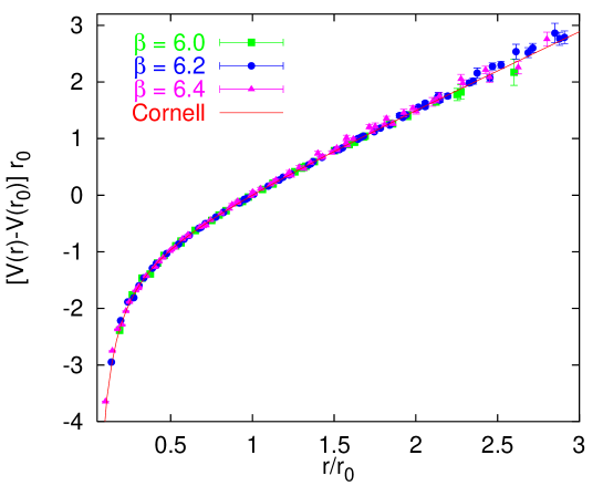
Figure 3: The quenched Wilson action $SU(3)$ potential in (3+1) dimensions, normalized to $V(r_{0})=0$.

The figure is taken from [85] (to which we refer for a thorough discussion of the interquark potential) and is a a compilation of data reported in Refs [27, 28].

Let us briefly comment this figure. This will also give us the opportunity to explain how LGT results are usually presented in the literature.

• Both the potential and the interquark distance are measured in units of $r_{0}$. This scale is obtained by looking at the intermediate range in the interquark potential. While the large-$r$ part of the potential is characterized by the string tension $\sigma$, one can characterize its behaviour at intermediate distances by the distance $r_{0}$ at which the force, $F$, has a particular value. It has become customary to use the particular definition $r_{0}^{2}F(r_{0})=1.65$ (which corresponds to a value that can be calculated with precision on the lattice and which can be estimated with some reliability from the observed spectrum of heavy quark systems). In physical units this corresponds to $r_{0}\approx 0.5$ fm.

• The important consequence of this choice is that in this way all the physical quantities ($r$ and $V(r)$) are measured in physical units and not in terms of the lattice spacing. The whole complexity of the scaling function eq.(33) is hidden in $r_{0}$ and the two combinations $r/r_{0}$ and $V(r)r_{0}$ are adimensional ratios, in the sense discussed in sect. 3.3. They are renormalization group invariant quantities and must keep the same value as the cutoff is changed (or, that is the same, as $\beta$ is changed) if we are in the scaling region. Thus we have an immediate and very effective test of scaling: data taken at different values of $\beta$ must overlap in the figure.

• This is indeed the case for the data reported in the figure which correspond to three samples of data (denoted by squares, triangles and circles respectively), obtained with MC simulations performed at three different values of $\beta$ (see the inset in the figure). The perfect overlap of the data is telling us that, at least for this observable, the scaling region is reached already at $\beta=6.0$.

• By using the scaling function (and the value $r_{0}\approx 0.5$ fm) we may obtain the value, in physical units, of the lattice spacing for the three samples in the figures. They correspond to $a\approx 0.094$ fm, 0.069 fm and 0.051 fm, respectively. This gives an idea of the size of the “grid” of our lattice approximation.

• Looking at the figure we see that the maximum interquark distance that we one can study is about 1.5 fm (recall that we are in the quenched approximation, so the interquark string cannot break). If we tried to push the quark and antiquark pair further apart we would have to face two types of problems. First we would have to fight against increasing statistical errors (denoted in the figure by the errors bars) due to the fact that as the Wilson loops become larger and larger, since they are exponentially depressed due to the area law, the signal to noise ratio becomes smaller and smaller and too long runs are needed to obtain statistically significant results. Second, one must take into account the systematic errors due to the finite size of the lattice in which the Wilson loops are immersed. The lattice size must be much larger than the Wilson loop size to allow one to neglect these systematic errors, but again larger lattices require much more time to obtain statistical independent configurations.

• The data are fitted with the so called “Cornell potential”, which is essentially eq.(54) in which the coefficient of the $1/R$ term is kept as a free parameter:

  $$V(r)=V_{self}+\sigma r-\frac{e}{r}$$ (55)

  The result of the two parameter fit is plotted in the figure as a continuous line. One can directly see that the data agree very well with the proposed function. The best fit value for $e$ is $e=0.295$ which is slightly higher than the bosonic string prediction. This could be due to the interplay with the one gluon exchange contribution or to the fact that in the Cornell approximation one is neglecting the subleading (log type) contributions of the effective string. However it could also be the signature that the effective string description of the model is more complicated than the simple free bosonic model.

• From the fit we also obtain a best fit estimate for the string tension. This is the value that we shall use in the next subsection as a scale to measure the glueball masses. We report in tab. 2 the result for both $SU(2)$ and $SU(3)$ in units of $\Lambda_{\overline{MS}}$. We also report in the same table for comparison the string tension in units of $r_{0}$ and $T_{c}$ (the deconfinement temperature).

• Looking carefully at the figure one can see that at small distances the data points lie somewhat above the curve, indicating a weakening of the effective coupling. This is a signature of the onset of asymptotic freedom at short distances.

	$SU(2)$	$SU(3)$
$r_{0}\sqrt{\sigma}$	$1.201\pm 0.055$	$1.195\pm 0.010$
$T_{c}/\sqrt{\sigma}$	$0.694\pm 0.018$	$0.640\pm 0.015$
$\Lambda_{\overline{MS}}/\sqrt{\sigma}$		$0.531\pm 0.045$

Table 2: Continuum limit value of the adimensional ratios of the string tension with the scale $r_{0}$, the deconfining temperature, $T_{c}$ and the (zero-flavour) $\Lambda$ parameter in the ${\overline{MS}}$ scheme for the $SU(2)$ and $SU(3)$ $YM$ theories in (3+1) dimensions.

The next step is now to study the large $N$ limit of the string tension. We shall address this problem in the simpler case of (2+1) dimensional theories

3.6.2 (2+1) dimensions

The analysis is similar to that discussed in the previous section, but in this case it is possible to perform simulations also for larger values of $N$ in particular, in [83] results for $N=4$ and $N=5$ were obtained. It turns out that these values are already large enough to perform a reliable large $N$ limit. Recall that in this case the coupling constant has the dimensions of a mass and thus can be used to set the mass scale of the whole theory.

It is thus natural in this case to express the string tension in units of $g^{2}$. The results for the various groups are:

$${{\sqrt{\sigma}}\over{g^{2}}}=\left\{\begin{array}[]{ll}0.3353(18)&\ \ \ \mbox{SU(2)}\\ 0.5530(20)&\ \ \ \mbox{SU(3)}\\ 0.7581(40)&\ \ \ \mbox{SU(4)}\\ 0.9657(54)&\ \ \ \mbox{SU(5)}\end{array}\right.$$ (56)

It is easy to see that these values increase linearly as a function of $N$. This agrees with the discussion of sect. 3.4 on the large $N$ limit where it was shown that the natural coupling in this limit is the ’t Hooft combination $g^{2}N$.

If we try to fit the data of eq.(56) keeping also into account the first subleading term in $1/N$ we see that it is proportional to $1/N^{2}$. This too is a prediction of the large $N$ analysis which is perfectly confirmed by the simulations.

The fit with two free parameters to the equation:

$${{\sqrt{\sigma}}\over{g^{2}N}}=c_{0}+{{c_{1}}\over{N^{2}}}$$ (57)

gives as a result:

$$c_{0}=0.1975(10)~{}~{},~{}~{}~{}~{}~{}~{}~{}~{}~{}~{}~{}~{}~{}~{}~{}~{}~{}c_{1}=-0.119(8)~{}~{}~{}.$$ (58)

with a very good confidence level (see [83] for the details). The value of $c_{0}$ obtained in this way represents the first example of a non-perturbative result in the large $N$ limit $SU(N)$ gauge theories.

Let us conclude with two comments on this result

• The fit gives an acceptable confidence level even if the $SU(2)$ result is taken into account, this means that the large $N$ limit analysis (taking into account also the first $1/N^{2}$ correction) holds all the way down to $N=2$

• The fact that the data show the correct $N$ dependence is a highly non trivial test of ’t Hooft analysis, since it comes from a truly non-perturbative regularization and is completely independent from the weak coupling arguments of sect. 3.4

3.6.3 The space-like string tension in finite temperature LGT.

It is important to stress that the results discussed in the two previous sections strictly refer to the zero-temperature version of $SU(N)$ LGT. In finite temperature LGT the interquark potential is obtained from the connected correlator of Polyakov loops. Recall that in FTLGT the lattice is asymmetric and we can distinguish between time-like and space-like Wilson loops. The spacelike Wilson loops are those orthogonal to the compactified time direction. If periodic boundary conditions in the time directions are imposed a timelike Wilson loop whose length in the $T$ directions is larger that the lattice size naturally becomes a pair of Polyakov loops, and this is the true order parameter for confinement. On the contrary the spacelike string tension is no longer an order parameter of the theory. In general it is different from zero even in the deconfined phase and (contrary to the naive expectation) increases as the temperature is increased! (for a discussion of this issue see for instance [29]). It will be important to remember this fact when we shall look at the Wilson loops in the framework of the AdS/CFT correspondence for non-supersymmetric gauge theories. It will turn out that they are actually spacelike Wilson loops of the underlying supersymmetric gauge theories. This explains why, while the supersymmetric theories, being conformally invariant, are not confining the spacelike Wilson loops (which will be interpreted as ordinary Wilson loops of the non-supersymmetric theory) are indeed confining.

3.7 The glueball spectrum.

3.7.1 (3+1) dimensions.

In this section we summarize our present knowledge of the glueball spectrum in (3+1) dimensions in the quenched approximation from Montecarlo simulations. The quantum numbers are presented with the standard convention $J^{PC}$ while the asterisks refer to the radial excitations. The most precise results have been obtained in the case of the $SU(2)$ and $SU(3)$ groups. They are reported in tab. 3 for $SU(2)$ and in tab. 4 for $SU(3)$. We take this opportunity to show some of the ways in which these data are usually presented in the lattice literature. In tab. 3 the glueball masses for the $SU(2)$ model are reported in units of the string tension (second column) and in units of the lowest glueball (last column). Notice the absence of any $C=-$ states in the $SU(2)$ case. These values are taken from ref. [84] and the quoted errors take care both of the statistical and the systematic uncertainties.

In tab. 4 we report the glueball spectrum for $SU(3)$ first (in the second column) in units of the scale $r_{0}$ (see the discussion in sect. 3.6.1) and then (last column) in physical units (MeVs). These values are taken from ref. [30]. The $SU(3)$ data are also plotted in fig. 4 (taken again from Ref. [30]). The width of the states in the figure corresponds to the combined statistical and systematic uncertainties of the estimates.

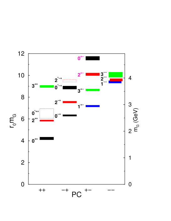
Figure 4: The glueball spectrum of $SU(3)$ gauge theory in (3+1) dimensions.

Let us stress an important non-trivial feature of the spectrum. Contrary to the naive expectations the $2^{++}$ state has a mass lower than that of the $1^{-+}$. This is not an accident, it happens in all the model studied up to now (both in (2+1) and (3+1) dimensions, both with continuous and discrete gauge groups) and can be considered as a fingerprint of $YM$ theories. We shall come back to this point when discussing the glueball spectrum in the AdS/CFT framework.

$J^{PC}$	$m_{G}/\sqrt{\sigma}$	$m_{G}/m_{0^{++}}$
$0^{++}$	3.74$\pm$0.12
$2^{++}$	5.62$\pm$0.26	$1.46\pm 0.09$
$0^{-+}$	6.53$\pm$0.56	$1.78\pm 0.24$
$2^{-+}$	7.46$\pm$0.50	$2.03\pm 0.20$
$1^{++}$	10.2$\pm$0.5	$2.75\pm 0.15$
$1^{-+}$	[10.4$\pm$0.7]	[$3.03\pm 0.31$]
$3^{++}$	9.0$\pm$0.7	$2.46\pm 0.23$
$3^{-+}$	[9.8$\pm 1.4$]	[$2.91\pm 0.47$]

Table 3: Continuum limit extrapolation for the glueball masses for the $SU(2)$ $YM$ theory in (3+1) dimensions. In the second column the masses are listed in units of the string tension, in the last column in units of the lightest scalar glueball mass. Values in brackets have been obtained by extrapolating from only two lattice values and so should be treated with caution.

$J^{PC}$	$r_{0}m_{G}$	$m_{G}$ (MeV)
$0^{++}$	4.21 (11)(4)	1730 (50)  (80)
$2^{++}$	5.85 (2)  (6)	2400 (25)  (120)
$0^{-+}$	6.33 (7)  (6)	2590 (40)  (130)
$0^{*++}$	6.50 (44)(7)†	2670 (180)(130)
$1^{+-}$	7.18 (4)  (7)	2940 (30)  (140)
$2^{-+}$	7.55 (3)  (8)	3100 (30)  (150)
$3^{+-}$	8.66 (4)  (9)	3550 (40)  (170)
$0^{*-+}$	8.88 (11)(9)	3640 (60)  (180)
$3^{++}$	8.99 (4)  (9)	3690 (40)  (180)
$1^{--}$	9.40 (6)  (9)	3850 (50)  (190)
$2^{*-+}$	9.50 (4)  (9)	3890 (40)  (190)
$2^{--}$	9.59 (4)  (10)	3930 (40)  (190)
$3^{--}$	10.06 (21)(10)	4130 (90)  (200)
$2^{+-}$	10.10 (7)  (10)	4140 (50)  (200)
$0^{+-}$	11.57 (12)(12)	4740 (70)  (230)

Table 4: Continuum limit extrapolation for the glueball masses for the $SU(2)$ $YM$ theory in (3+1) dimensions. In the second column the masses are listed in units of the $r_{0}$. The first error is the statistical uncertainty from the continuum-limit extrapolation and the second is an estimate of the systematic error due to the particular method (regularization on anisotropic lattices) used to evaluate the masses. In the last column the masses are reported in physical units. In this case the first error comes from the combined uncertainties in $r_{0}m_{G}$, the second from the uncertainty in $r_{0}^{-1}=410(20)$ MeV.

Let us now study the large $N$ limit of the glueball spectrum. As we did in the case of the string tension we shall first address the problem in the (2+1) dimensional case where everything is much simpler and under control. We shall then try in sect. 3.7.3 below to perform the same analysis in the more interesting (3+1) dimensional case.

$m_{G}/\sqrt{\sigma}$
state	$SU(2)$	$SU(3)$	$SU(4)$	$SU(5)$
$0^{++}$	4.718(43)	4.329(41)	4.236(50)	4.184(55)
$0^{++\ast}$	6.83(10)	6.52(9)	6.38(13)	6.20(13)
$0^{++\ast\ast}$	8.15(15)	8.23(17)	8.05(22)	7.85(22)
$0^{--}$		6.48(9)	6.271(95)	6.03(18)
$0^{--\ast}$		8.15(16)	7.86(20)	7.87(25)
$0^{--\ast\ast}$		9.81(26)	9.21(30)	9.51(41)
$0^{-+}$	9.95(32)	9.30(25)	9.31(28)	9.19(29)
$0^{+-}$		10.52(28)	10.35(50)	9.43(75)
$2^{++}$	7.82(14)	7.13(12)	7.15(13)	7.19(20)
$2^{++\ast}$			8.51(20)	8.59(18)
$2^{-+}$	7.86(14)	7.36(11)	6.86(18)	7.18(16)
$2^{-+\ast}$		8.80(20)	8.75(28)	8.67(24)
$2^{--}$		8.75(17)	8.22(32)	8.24(21)
$2^{--\ast}$		10.31(27)	9.91(41)	9.79(45)
$2^{+-}$		8.38(21)	8.33(25)	8.02(40)
$2^{+-\ast}$		10.51(30)	10.64(60)	9.97(55)
$1^{++}$	10.42(34)	10.22(24)	9.91(36)	10.26(50)
$1^{-+}$	11.13(42)	10.19(27)	10.85(55)	10.28(34)
$1^{--}$		9.86(23)	9.50(35)	9.65(40)
$1^{+-}$		10.41(36)	9.70(45)	9.93(44)

Table 5: Continuum limit values of the glueball masses for various (2+1) dimensional $SU(N)$ theories in units of the string tension.

state	$\lim_{N\to\infty}m/\sqrt{\sigma}$
$0^{++}$	4.065(55)
$0^{++\ast}$	6.18(13)
$0^{++\ast\ast}$	7.99(22)
$0^{-+}$	9.02(30)
$2^{++}$	6.88(16)
$2^{-+}$	6.89(21)
$2^{-+\ast}$	8.62(38)
$1^{++}$	9.98(25)
$1^{-+}$	10.06(40)
$0^{--}$	5.91(25)
$0^{--\ast}$	7.63(37)
$0^{--\ast\ast}$	8.96(65)
$0^{+-}$	9.47(116)
$2^{--}$	7.89(35)
$2^{--\ast}$	9.46(66)
$2^{+-}$	8.04(50)
$2^{+-\ast}$	9.97(91)
$1^{--}$	9.36(60)
$1^{+-}$	9.43(75)

Table 6: The large $N$ limit of the mass spectrum in units of the string tension in (2+1) dimension.

3.7.2 (2+1) dimensions.

We report in tab. 5 the glueball spectrum in units of the square root of the string tension for $N=2,3,4$ and $5$. The table is taken from [83]. As anticipated above we observe again the inversion between the states of the $J=2$ family and those of the $J=1$ one. The fact that in this case also $N=5$ data exist allows to make a reliable large $N$ limit analysis. Thus, following the discussion of sect. 3.6.2 let us fit these data with

$${{M(J^{PC})}_{N}\over{g^{2}N}}=M(J^{PC})_{\infty}+{{d_{1}}\over{N^{2}}}$$ (59)

where we denote with $M(J^{PC})_{N}$ the mass of the glueball of quantum numbers $J^{PC}$ in the $SU(N)$ theory.

For all the $J^{PC}$ values the fits turn out to have good confidence levels. The large $N$ limit results are reported in tab. 6 (in units of the large $N$ string tension). In the upper part of the table we have listed the glueball states with $C=+$ for which also $SU(2)$ data exist. In the lower part of the table we report the $C=-$ states which are obtained by fitting only data with $N>2$. These are the numbers with which we shall compare the AdS/CFT predictions for (2+1) dimensions which we shall discuss in the next section.

$SU(4)$
	$\beta=10.7$	$\beta=10.9$	$\beta=11.1$
$a\sqrt{\sigma}$	$0.296\pm 0.015$	$0.228\pm 0.007$	$0.197\pm 0.008$
$am_{0^{++}}$	$0.98\pm 0.17$	$0.75\pm 0.07$	$0.77\pm 0.06$
$am_{0^{++\star}}$	$1.54\pm 0.44$	$1.39\pm 0.16$	$1.03\pm 0.14$
$am_{2^{++}}$	$1.28\pm 0.27$	$1.21\pm 0.11$	$1.04\pm 0.12$

Table 7: $SU(4)$ masses and string tensions in(3+1) dimensions on $10^{4}$, $12^{4}$ and $16^{4}$ lattices at $\beta=$10.7, 10.9 and 11.1 respectively.

$SU(\infty)$
$m_{0^{++}}/\sqrt{\sigma}$	$3.56\pm 0.18$
$m_{2^{++}}/\sqrt{\sigma}$	$4.81\pm 0.35$
$T_{c}/\sqrt{\sigma}$	$0.597\pm 0.030$
$r_{0}\sqrt{\sigma}$	$1.190\pm 0.043$

Table 8: Various adimensional ratios in (3+1) dimensions, after extrapolation to $N=\infty$ from $N=2$, $N=3$ and $N=4$; $assuming$ the validity of eqn(60) all the way down to $N=2$.

3.7.3 Large $N$ limit in 3+1 dimensions

In order to perform a reasonable large $N$ limit also in (3+1) dimensions we need at least few informations also on the $SU(4)$ theory. In Tab. 7 are reported some of the existing data for $SU(4)$ taken from [84]. They deal only with the lowest three states of the spectrum, but at least for them, they allow a tentative large N extrapolation.

In fact we see from tables 3,4 and 7 that the physical properties of $SU(2)$, $SU(3)$ and $SU(4)$ gauge theories are very similar. Assuming, as in the $2+1$ dimensional case that we are already close to the $N=\infty$ limit even with $N=2,3,4$ we can extrapolate the glueball masses (in units of $\sqrt{\sigma}$) to the $N=\infty$ limit using

$${m\over{\sqrt{\sigma}}}\Biggl{|}_{\!N}={m\over{\sqrt{\sigma}}}\Biggl{|}_{\!\infty}+\ {c\over{N^{2}}}$$ (60)

In this way we obtain the values displayed in table 8 (see [84] for the details). While these results are slightly less stable than the (2+1) dimensional ones they represent nevertheless the first non-perturbative results in the large $N$ limit of $SU(N)$ gauge theories in (3+1) dimensions. As such they are of the greatest importance. We shall use them to discuss the validity of the AdS/CFT approach in the (3+1) dimensional case in the next section.

4 AdS/CFT.

As we mentioned in the introduction we shall assume in the following that the reader is already acquainted with the theory behind the AdS/CFT correspondence. Some good reviews exist on the subject [87, 88] where the interested reader can find a thorough discussion of the correspondence and all the needed background material. The aim of this section is to provide the reader with the necessary information to compare the physical picture which emerges in the framework of the AdS/CFT correspondence with the results discussed in the previous sections following the lattice approach. For this reason we have organized this section in two parts: in the first one (sect. 4.1) we shall state the conjecture and discuss a few basic results (in particular on its finite temperature version) which will be needed in the following. In the second part (sect. 4.2 and 4.3) we shall review those results which are relevant for a comparison with the lattice. In particular, in sect. 4.2 we shall only deal with the finite temperature (i.e. non-supersymmetric) realization of the correspondence but, in this restricted field, we shall try to keep our review as complete as possible. In sect. 4.3 we shall mention a few results concerning the supersymmetric theory (i.e. the zero temperature case) which, due to their generality, could be (despite the presence of supersymmetry) of some importance for the comparison that we are discussing.

4.1 The AdS/CFT correspondence.

It is very important to stress that in going from string theory to QCD along the lines that we are discussing now, two distinct steps are needed.

The first one is the AdS/CFT correspondence, based on the Maldacena conjecture [8], and further specified in the works of Witten [31] and Gubser, Klebanov and Polyakov [32] . This correspondence relates string theories on suitably chosen AdS manifolds with conformally invariant field theories whose symmetries depend on the internal manifold.

The second step is the breaking of conformal invariance and (if present) of supersymmetry, in order to obtain a candidate for a QCD-like theory. In these lectures we shall follow the proposal of Witten [9], in which a QCD-like theory is obtained by compactifying the original theory with suitable boundary conditions. This proposal has several appealing features and originated a large amount of papers, but it is not the unique possible choice. We shall briefly comment on this further freedom below.

Let us now discuss in more detail these two steps.

• The Maldacena conjecture relates the $M$ theory (or, depending on the case, one of its superstring limits) in the $AdS_{d+1}\times{\bf X}$ background to the large $N$ limit of a $d$ dimensional conformal field theory. ${\bf X}$ is an Einstein manifold whose particular form depends on the type of field theory which we are interested to describe. In particular, by suitably choosing ${\bf X}$ it is possible to induce the presence on the field theoretic side of the correspondence of supersymmetry, or of a $SU(N)$ gauge symmetry. It is important to stress that, independently from the choice of the background, the resulting field theory is always conformally invariant (this explains the abbreviation AdS/CFT which is used to denote this correspondence) and, as a consequence, is not confining.

  In the following we shall only discuss this correspondence in two cases

  1] In the first case we choose on the string side a type IIB superstring in the $AdS_{5}\times{\bf S^{5}}$ background. The corresponding field theory turns out to be the large $N$ limit of the $SU(N)$ ${\cal N}=4$ supersymmetric gauge theory in 4 dimensions. This will be the starting point to obtain, following Witten’s suggestion a candidate for a three dimensional non-supersymmetric YM theory

  2] In the second case we choose to study, on the string side, $M$ theory on a $AdS_{7}\times{\bf S^{4}}$ background. This theory is mapped by the Maldacena conjecture to the large $N$ limit of a a six dimensional $SU(N)$ type $(2,0)$ theory which is again supersymmetric and conformally invariant. By compactifying the theory in two directions according to Witten’s proposal we shall then obtain a candidate for a four dimensional non-supersymmetric YM theory

  It is important to stress that this AdS/CFT correspondence is formally only a conjecture. As a matter of fact one can recognize three levels of this conjecture. Let us discuss them in the most studied example of type IIB string in the $AdS_{5}\times{\bf S^{5}}$ background (case 1 in the above list)

  a] In this case the “weak” statement is that the correspondence only holds between supergravity on $AdS_{5}\times{\bf S^{5}}$ and the strong coupling limit of large $N$ $SU(N)$ ${\cal N}=4$ supersymmetric gauge theory in 4 dimensions (this is the “supergravity limit” that we shall discuss below). This level of the conjecture has obtained by now so many confirmations (see for instance [88] for a thorough discussion of all these checks) that it is commonly accepted as a firmly established result.

  b] The “normal” level of the conjecture is the one that we have stated at the beginning of this section. It extends the relation from the supergravity limit to the whole type IIB superstring in the $AdS_{5}\times{\bf S^{5}}$ background, which is related with the large $N$ limit of the $SU(N)$ ${\cal N}=4$, with no constraint on the gauge coupling. This means that, with respect to the “weak” interpretation we are now pushing the correspondence outside the strong coupling limit. If we want to to obtain from the AdS/CFT correspondence a QCD-like theory in the weak coupling limit (which is the ultimate goal of these lectures), we must at least invoke this level of the conjecture. This is usually implicitly assumed in most of the papers that we shall discuss below. However essentially no check exists of the Maldacena conjecture at this level.

  c] The “strong” level consists in assuming that the conjecture holds also for the string theory at an arbitrary order in the loop expansion. From the field theory side this would imply that we have informations not only in the $N\to\infty$ limit but to any order in the $1/N$ expansion. As we have seen in sect. 3, this is actually not so important since we have by now a rather good control of the large $N$ limit on the Lattice side.

  It is worthwhile to stress that (independently from the possible applications to QCD) the AdS/CFT correspondence is of great theoretical interest in itself. In some sense it represents the first nontrivial case in which we have been able to find the master field solution of a $d>2$ dimensional gauge theory in the large $N$ limit.

  At the same time it is the first explicit description of a $d>2$ gauge theory in terms of a string theory. It seems somehow paradoxical that this remarkable result has been obtained for the first time in the case of a gauge theory which is not confining while the string description of gauge theories has been based, from the very beginning, on the intuitive picture of a string configuration spanning the minimal area of a confining Wilson loop. The mechanism behind this apparent contradiction is very instructive. The intuitive picture is indeed correct and also in the present case the string is spanning the minimal area of the Wilson loop. However due to the peculiar properties of the $AdS$ space the world-sheet of the string, in order to minimize its area must wander deep into the extra dimensions. This destroys the linear confining potential and leads to an effective $1/R$ behaviour.

• If we aim to reach a description of real QCD-like theories it is mandatory to break the conformal invariance discussed above so as to recover a well behaved confining potential. At the same time (if needed) we must somehow break the supersymmetry of the theory . There are several possible ways to obtain these two results and we refer to [88] and [87] to a discussion of these options. In the rest of these lectures we shall concentrate on the proposal suggested by Witten in [9]. The main appealing feature of this proposal is its simplicity, however one must always keep in mind that it is not the unique possibility. In principle some of the problems that we shall discuss below and that seem to make impossible a successful comparison with standard YM theories could be avoided following other routes.

  Following [9], we can break the conformal invariance of the theory by compactifying the theory in one (or more) direction(s). The presence of a new scale (the compactification radius) in the problem automatically breaks conformal invariance. If we then choose antiperiodic boundary conditions for the fermions in (one of) the compactified directions we also break supersymmetry. In fact as a consequence of the antiperiodic boundary conditions the gauginos and and the adjoint scalars acquire a nonzero mass. The important point in all these steps is that the Maldacena conjecture can be extended also to the compactified version of the theory thus allowing to have an insight in the infrared regime of the resulting gauge theory also in this case. It is also important to stress, so as to avoid confusion, that the theory obtained in this way is good candidate for a pure Yang Mills theory. The term QCD which is often used in the literature is from this point of view rather misleading.

Let us now study the two interesting examples of $YM_{3}$ and $YM_{4}$. We choose to study first the case of 3d $YM$ which, for some technical reason turns out to be simpler, we shall later generalize the results to the more interesting case of 4d $YM$.

4.1.1 The simplest example: $YM_{3}$

In this case we must start by studying type IIB superstring in the $AdS_{5}\times{\bf S^{5}}$ background. The Maldacena conjecture allows then to relate this theory with the large $N$ limit of the $SU(N)$ ${\cal N}=4$ supersymmetric gauge theory in 4 dimensions. The pattern suggested by Witten to break conformal invariance and supersymmetry is very simple in this case. Both these goals can be reached, by compactifying only one direction. There is a nice physical interpretation of this recipe. If we choose to compactify the manifold in the time direction then Witten’s proposal is equivalent to study the original system at a nonzero temperature $T$, proportional to the inverse of the compactification radius $R_{0}$. For this reason we shall often call in the following the original $SYM$ theories as $T=0$ theories and the non-supersymmetric compactified ones as $T>0$ theories. In the $R_{0}\to 0$ (hence $T\to\infty$) limit we then obtain a three dimensional effective theory which has several features in common with large $N$ 3d $YM$ and could hopefully be identified (at least in some limit) with it.

Few comments are in order at this point:

Coupling constants.

It is important to follow the coupling constant identifications that emerge from the two above steps. Let us define the coupling constant of the ${\cal N}=4$ $SU(N)$ theory as $g_{YM,~{}({\cal N}=4)}^{(4)}$. The Maldacena conjecture tells us that $(g_{YM,~{}({\cal N}=4)}^{(4)})^{2}$ is proportional to the string coupling $g_{s}$. We have seen in sect. 3.4 that the large $N$ limit must be taken keeping the ’t Hooft coupling $\lambda\equiv Ng^{2}_{YM}$ finite. In the present case the ’t Hooft coupling is $\lambda\equiv N(g_{YM,~{}({\cal N}=4)}^{(4)})^{2}$. The coupling constant of the three dimensional compactified theory can be expressed in terms of the four dimensional one as follows (this is a standard result in finite temperature gauge theories):

$$N(g_{YM}^{(3)})^{2}=\frac{N(g_{YM,~{}({\cal N}=4)}^{(4)})^{2}}{R_{0}}$$ (61)

Thus while the original coupling $N(g_{YM,~{}({\cal N}=4)}^{(4)})^{2}$ was dimensionless the 3d one has the dimensions of a mass, which completely agrees with the expected behaviour of $YM_{3}$ (see sect. 2.3). In the rest of this review we shall adopt the following convention to distinguish among the various ’t Hooft couplings. We shall denote with $\tilde{\lambda}_{d}$ the couplings which refer to the original $T=0$ supersymmetric $YM$ theories, where $d$ refers to the dimension of the theory, while we shall denote with $\lambda_{d}$ the coupling of the compactified non-supersymmetric theories. In this last case $d$ will denote the number of uncompactified dimensions. Thus in the present case:

$$\tilde{\lambda}_{4}\equiv N(g_{YM,~{}({\cal N}=4)}^{(4)})^{2}~{}~{}~{},\hskip 28.45274pt\lambda_{3}\equiv N(g_{YM}^{(3)})^{2}~{}~{}.$$ (62)

So that eq.(61) becomes

$$\lambda_{3}=\frac{\tilde{\lambda}_{4}}{R_{0}}$$ (63)

The supergravity limit.

A crucial point for the following discussion is that we are actually unable to study the string theory on the AdS manifold in its full complexity. As a matter of fact we are bound to study the so called supergravity limit, in which the string excitations are negligible and the string theory reduces to supergravity. From the AdS/CFT correspondence one can see that this region corresponds to the $\tilde{\lambda}_{4}>>1$ regime of the ${\cal N}=4$ $SU(N)$ theory. In this limit the AdS/CFT correspondence is rather well understood: it essential amounts to a correspondence between supergravity fields on one side and local operators of the gauge theory on the other side. The problem is that in this limit we may only have informations on the strong coupling sector of the gauge theory. If we now move to the compactified theory we face exactly the same problem. By using supergravity we may only have informations on the strong coupling regime of the theory that we hope to identify with $YM_{3}$.

Kaluza-Klein states.

Another relevant problem is represented by the fact that in compactifying the $S_{5}$ part of the original ten dimensional supergravity on $AdS_{5}\times S_{5}$ a lot of Kaluza-Klein (K-K in the following) states are generated. Most of them have no counterpart in ordinary $YM$ theories and are expected to decouple in the $\lambda_{3}\to 0$ limit. However in the limit in which the calculations can be performed there is still no evidence of such a decoupling. We shall come back to this problem when dealing with the glueball spectrum below.

Beyond supergravity.

We have already said (and will repeat several time in the following) that in order to test in a reliable way the predictions obtained from the AdS/CFT correspondence we would need to extend them to the weak coupling regime of the theory. The quest for such an extension will appear in all the tests that we shall discuss below. However for small values of $\tilde{\lambda}_{4}$ the background geometry develops a singular behaviour and the supergravity approximation breaks down. In this regime one has to study the string theory on the AdS manifold in its full complexity. This means in particular that one should be able to study the string theory with background Ramond-Ramond charge in a singular background geometry. Despite several efforts few progress have been made in this direction up to now. However it is important to stress that this seems to be only a technical and not a conceptual obstacle and that it is well possible that in future this barrier could be overcome.

4.1.2 Extension to $YM_{4}$

One can follow a procedure similar to the one outlined above to obtain a non-supersymmetric four dimensional gauge theory which could hopefully be in the same universality class of $YM_{4}$. This time one must start by looking at the $M$ theory in the $AdS_{7}\times S_{4}$ background. This theory is mapped by the Maldacena conjecture to the large $N$ limit of a a six dimensional $SU(N)$ type $(2,0)$ theory which is supersymmetric and conformally invariant. By compactifying the theory in two directions we then reach the desired four dimensional $SU(N)$ gauge theory. As a consequence of the compactification both supersymmetry and conformal invariance are lost, as it happened in the three dimensional case. However this time the relationship between the six dimensional gauge coupling and the four dimensional one is much more subtle. Let us see this correspondence in more detail. Let us denote with $R_{1}$ and $R_{2}$ the two compactification radii. In order to obtain a reduced theory with the same features of $YM_{4}$, supersymmetry must be broken only in one of the two directions, let us choose it to be the one with radius $R_{2}$, while $R_{1}$ will be the radius of the supersymmetry preserving circle. Then the four dimensional gauge coupling constant $g^{(4)}_{YM}$ is given by:

$$(g^{(4)}_{YM})^{2}=\frac{R_{1}}{R_{2}}$$ (64)

which is adimensional, as in $YM_{4}$. In order to reach the four dimensional theory that we hope to identify with $YM_{4}$ both the radii must be sent to zero, however their role is very different. Since in the large $N$ limit we want to keep the ’t Hooft coupling $\lambda_{4}=N(g^{(4)}_{YM})^{2}$ to be finite, $R_{1}$ must go to zero in the large $N$ limit much faster than $R_{2}$. The remaining scale $R_{2}$ plays the role of an ultraviolet cutoff for the four dimensional theory. Thus the gauge coupling $g^{(4)}_{YM}$ must be thought of as the bare coupling at distances of order $R_{2}$, and all dimensional quantities must be measured in units of $R_{2}$. Remarkably enough the situation is exactly the same that we have in LGT, with $R_{2}$ playing the same role of the lattice spacing in LGT.

If we aim to identify the theory that we have found with $YM_{4}$, we must require that, in the $R_{2}\to 0$ limit, $\lambda_{4}$ scales as follows:

$$\lambda_{4}\to-\frac{b}{\log(\Lambda_{QCD}R_{2})}$$ (65)

with $b$ a suitable constant dictated by the Callan Symanzik equation.

However, exactly as in the three dimensional case discussed above we are only able to study the large $\lambda_{4}$ regime of the theory and any test of a behaviour like that of eq.(65) is well beyond our present control of theory. Again, we are bound to study the strong coupling regime of the theory.

There are at this point two possible options: the first one is to try to infer the small $\lambda_{4}$ behaviour of theory from the strong coupling informations that we have. The second is to try to extrapolate real $YM$ to the strong coupling limit and then compare with our findings. In both these approaches the comparison with the lattice results plays a crucial role.

4.2 Review of the results for the non-supersymmetric theories

All the attempts which have been made up to now to compare the results obtained in the framework of the finite temperature version of AdS/CFT correspondence with $YM$ theories dealt with essentially only two topics: the glueball spectrum and the string tension. The present status of these calculations is rather controversial. While a substantial agreement on the general pattern of both the glueball spectrum and the string tension has been achieved, some conflicting results still exist and the whole issue is still evolving. In particular, the agreement with the LGT results which was claimed at the beginning has been lost in the most recent analyses. For this reason we shall avoid to collect in a table a tentative list of mass values as we did when reviewing the LGT results. Instead we shall devote the next two sections to a review of the various attempts and results together with the open problems. We shall then conclude by listing the general features on which a consensus has been reached. Let us finally mention that in the following we shall write the coupling dependence of all the dimensional quantities as a function of $\lambda_{4}$ in the four dimensions case and as a function of $\tilde{\lambda}_{4}$ in the three dimensional one. The reason of this asymmetric choice is that both $\lambda_{4}$ and $\tilde{\lambda}_{4}$ are adimensional, and this greatly simplifies the discussion of the results.

4.2.1 Glueball spectrum.

In principle the calculation of the glueball spectrum, at least for the $0^{++}$ state, is rather simple. In the supergravity limit the $0^{++}$ glueball is mapped by the Maldacena conjecture into the dilaton field of the corresponding supergravity description. Its mass is then obtained by solving the dilaton wave equation. This calculation was first performed in [39, 40, 41] where the spectrum of the first excited states of the $0^{++}$ and $0^{--}$ states in $d=3$ and of the $0^{++}$ and $0^{-+}$ glueballs in $d=4$ was obtained. The result had the correct dependence on the ultraviolet cutoff ($R_{0}$ and $R_{2}$ respectively) and showed no explicit dependence on $\tilde{\lambda}_{4}$ or $\lambda_{4}$.

The numerical values of the lowest states turned out to be of order unity if measured in units of $1/R_{0}$ (or $1/R_{2}$). These values were then compared with LGT results  and a good agreement was claimed. However it later appeared that such a claim was probably not justified. In [42] the mass of the $2^{++}$ glueball (both in $3$ and in $4$ dimensions) was obtained and turned out to be degenerate with the $0^{++}$ one, a result which certainly disagree with the LGT estimate reported in tab.s 6 and 8.

At the same it was realized in [43] that in the three dimensional case the $0^{++}$ state associated with the graviton (in the supergravity limit) has a mass smaller than the one associated with the dilaton and hence must be considered as the lowest glueball state. If the various glueball masses are measured in units of this new fundamental mass, then the quantitative agreement with the LGT spectrum is definitely lost. However a “qualitative” agreement with lattice results is still present. In [43] the authors also evaluated the glueball state with quantum numbers $1^{-+}$ and it turns out that.

$$m(0^{++})<m(2^{++})<m(1^{-+})$$ (66)

which is exactly the same pattern which emerges in LGT. Let us stress that this is a rather non-trivial result. As mentioned in sect. 3.7 the fact that the $2^{++}$ state has a mass lower than that of the $1^{-+}$ one is a fingerprint of QCD.

The main problem of all these calculations is the presence of the unwanted Kaluza-Klein states discussed above. It turns out that in the supergravity limit the masses of these states are of the same order of those of the glueballs. As mentioned above this is nothing else that another signature that we are actually looking at the strong coupling regime of the theory. The approach to the problem followed in the papers discussed above was to simply neglect these states assuming that they should eventually decouple if one would be able to reach the weak coupling limit. However it was noticed in [44] that, at least in the first order in the string corrections, such a decoupling is not evident and the masses of the K-K states remain of the same order of that of the true glueball states.

It was thus proposed to study some suitable deformation of the supergravity theory which could eliminate right from the beginning these states. The idea is that there is not a unique realization of the strong coupling theory which we hope to identify with $YM$, but a whole family of theories which depend on one or more free parameters. Thus in principle we could tune these parameters so as make the theory as similar as possible to the weak coupling one. This is in some sense the same philosophy of the so called ”improved actions” in LGT. In this framework, the elimination of the K-K modes is certainly a step in the right direction.

This program was pursued in [45, 46, 47, 48] and more recently in in [49], Unfortunately only part of the K-K spectrum could be eliminated in this way. The glueball spectrum obtained in this framework depends in the most general case on three free parameters in $d=3$ [47] and two parameters in $d=4$ [48], however it turns out that the mass ratios are very stable as a function of these parameters. This interesting phenomenon, which points toward the presence of some kind of universal behaviour has been discussed in [50].

Let us conclude with a last, positive, observation. If one were able to extrapolate these mass gap calculations up to the weak coupling limit then one should observe the scaling behaviour of eq.(33). In [39] a first step has been made in this direction, by looking at the first string correction of the mass spectrum. The authors found that the corrections are negative. This means that, for a fixed ultraviolet cutoff the masses decrease as the ’t Hooft coupling $\lambda_{4}$ is decreased, in agreement with the expected behaviour of eq.(33).

Let us summarize the main results.

• Even if there is no quantitative agreement with the lattice estimates, the pattern of the glueball masses (at least in $d=3$) is correctly reproduced.

• The leading string corrections to the masses have the correct sign.

• The (dual) supergravity description of $YM$ can be generalized so as to incorporate two (or three) free parameters. The mass ratios show a negligible dependence on these parameters

4.2.2 String Tension.

As we discussed in the introduction to LGT (sect. 3.1.1) in order to estimate the string tension one must be able to evaluate the expectation value of Wilson loops of large size. This problem is completely different from the one discussed in the previous section and requires different tools. A method to compute these Wilson loops in Super Yang Mills theories via supergravity was suggested in [51, 52]. These ideas were then applied to the compactified theories in which we are interested in [53, 54] and (as already predicted in [9]) a confining, linearly rising potential was indeed found. It is important at this point to recall the discussion made in sect. 3.6.3 .

The Wilson loops which are studied in [53, 54] (and also in all the other papers that we shall discuss in this section) are the equivalent of what we called in sect. 3.6.3 “spacelike” Wilson loops. As such they do not give informations on the potential of the original theory (which in fact, as we know, is not confining) but only on the dimensionally reduced one. Since the original theory is not confining we expect a transition (or a smooth crossover) between the two behaviours as the compactification radius is shrunk to zero (i.e. as the temperature is increased).

Let us call $L$ the size of the Wilson loop (i.e. the distance between the quark and the antiquark), let us study first the case of the $d=4$ ${\cal N}=4$ theory compactified to three dimensions. We expect that a confining potential appears in the limit $\frac{L}{R_{0}}>>0$, i.e. when the distance between the quarks is much larger than the compactification radius. In the opposite limit $\frac{L}{R_{0}}<<0$ on the contrary we expect to recover the Coulomb like behaviour of the ${\cal N}=4$ $SYM$ in $d=4$. Indeed this is exactly the behaviour which was found in [53, 54]. In the large $L$ limit it is thus possible to extract the string tension whose value turns out to be

$$\sigma=\sqrt{\pi\tilde{\lambda}_{4}}\frac{\pi}{R_{0}^{2}}$$ (67)

A similar analysis can be performed also in four dimensions, leading to the following expression for the string tension:

$$\sigma=\frac{8\pi}{27}\frac{\lambda_{4}}{R_{2}^{2}}$$ (68)

Both eq.(67) and (68) show that the string tension has the correct dimensions of $(mass)^{2}$, however its dependence on the coupling constant shows that there is a serious problem in the whole calculation. Moreover it is rather puzzling the fact that there is no signature of a $1/L$ type term which in LGT arises from the quantum fluctuations of the effective string. Let us discuss these two problems in more detail.

The $\lambda$ dependence of $\sigma$

Let us address this problem directly in the four dimensional case. We saw in the previous section that the lowest glueball masses were of order unity if measured in units of $1/R_{2}$ and showed no dependence on $\lambda_{4}$. On the contrary the square root of the string tension measured in units of $1/R_{2}$ is proportional to $\sqrt{\lambda_{4}}$ which must be much larger than unity in the supergravity limit, which in turn is the only regime in which we can trust this solution. This has two unwanted consequences.

First of all it completely disagrees with what we expect from both $YM_{3}$ and $YM_{4}$ in the continuum limit (see sect. 3.7) where the ratio $\sqrt{\sigma}/M(0^{++})$ is of order unity.

Second, it is telling us that we are actually testing the QCD string at very short distances, much shorter than the compactification radius, i.e. in a regime in which in ordinary $YM$ theories we do not expect to observe a “string-like” behaviour which is instead a peculiar feature of the large distance infrared regime of Wilson loops.

As stressed in [57] the fact that $M(0^{++})$ and $\sqrt{\sigma}$ are of the same order of magnitude and have the same dependence on the bare coupling constant is an unavoidable consequence of the existence of a string-like description for the theory in which the glueballs come from closed strings. It is amazing that this property does not hold if we describe $YM$ theories in the framework of the AdS/CFT correspondence which is explicitly constructed to obtain a string description of $YM$ theories. As we have seen above, this can be interpreted as a consequence of the fact that with the AdS/CFT results we are actually probing the short range regime of the the Wilson loop and that the confining regime that we observe has little to do with the real large distance potential of the theory. Thus we may hope that also this problem will be solved when we shall be able to overcome the supergravity limit. An interesting proposal in this direction has been recently suggested in [58]. The main point is that a log term appears in the the string tension if the corrections induced by the quantum fluctuations of the string [59] are taken into account (we shall discuss in detail these corrections below, when dealing with the Lüscher term). The string tension becomes:

$$\sigma=\frac{8\pi}{27}\frac{\lambda_{4}}{R_{2}^{2}}+\frac{4\pi}{R_{2}^{2}}\log(R_{2}^{2}\mu^{2})+O(1/\lambda_{4})$$ (69)

where $\mu$ is an arbitrary scale which is introduced to regulate the sum over the modes of the string fluctuations. In principle we may use this additional term to eliminate the unwanted $\lambda_{4}$ dependence in $\sigma$ by suitably choosing the dependence of $\lambda_{4}$ on the ultraviolet cutoff $R_{2}$. If we want to have a string tension

$$\sigma=\frac{c^{2}}{R_{2}^{2}}$$ (70)

with some fixed constant $c$, such that the ratio $c/M(0^{++})$ agrees with the results from LGT we must impose:

$$\lambda_{4}=\frac{27c^{2}}{8\pi}-27\log(R_{2}\mu)$$ (71)

This behaviour is compatible with the other constraints on $R_{2}$ and $\lambda_{4}$ if $\mu<<\frac{1}{R_{2}}$. In this case the log term dominates over the constant and we recover the large $\lambda_{4}$ regime in which the result of eq.(68) was obtained. It is important to stress that eq.(71) imposes a constraint on the behaviour of the coupling constant $\lambda_{4}$ as a function of the ultraviolet cutoff which is different from the one due to asymptotic freedom (see eq.(65)). It can be shown [58] that these two constraints have somehow a symmetric role. They determine the behaviour of the coupling $\lambda_{4}$ as a function of the cutoff in the strong and in the weak coupling regime respectively.

The Lüscher term

We have seen in sect. 3.5 that the area law is only the first dominant term of the potential and that besides it we expect an universal subleading correction: the Lüscher term, which is due to the quantum fluctuations of the string. In the framework of the AdS calculations that we are discussing, in the supergravity limit, there is no signature of such a term. This problem was noticed and discussed in [57].

Once again a possible solution to the problem is that such a term could appear if higher order string-like corrections are taken into account. This type of calculations are very delicate since they require a careful treatment of the boundary conditions for the Wilson loop which in the finite temperature case is a rather non-trivial issue (see the comments in this respect in [55]and [56]). A tentative in this direction was performed in [59],[60] and [61] and a term with the desired $\frac{1}{L}$ behaviour was found, but with the wrong sign! .

In view of what we were saying before, i.e. of the fact that we are actually probing the short range regime of the Wilson loops, the lack of a Lüscher term is not surprising. The same would happen also in LGT, where the $1/L$ correction manifests itself only at distances much larger than the ultraviolet cutoff.

However the fact that an $1/L$ term is present, but with the wrong sign rises a different problem, which on the contrary seems to be rather serious. We have seen at the end of sect. 3.5.3 that a very general requirement for the potential is that it must be a concave function of the interquark distance [26] and a Lüscher term with the wrong sign violates this requirement [59]. This problem was studied in detail in [63] where the authors discuss which conditions must be imposed on a AdS type theory so as to fulfill the concavity requirement in the induced gauge theory.

4.3 A few results on the supersymmetric case.

String fluctuations in $AdS_{5}\times S^{5}$. As we mentioned above, the calculations on the Lüscher term discussed in the previous section are particularly delicate since they require a careful treatment of the boundary conditions for the Wilson loop. Recently some progress has been made in this respect in the zero temperature case. In particular in [56] a careful discussion of the semiclassical fluctuations of strings in $AdS_{5}\times S^{5}$ based on the Green-Schwarz formalism can be found. In this paper the authors also study, among other examples, the string corrections to the expectation value of the Wilson loop in the ${\cal N}=4$ Super Yang Mills theory in $d=4$.

Loop equations.

We have seen in sect. 3.4 that a basic feature of the large N limit of $SU(N)$ gauge theories is the fact that they satisfy the so called loop equations. The solution of these loop equations would be the sought for master field of the theory. Since these equations hold also in the strong coupling phase of the theory they are a perfect testground for the validity of the conjecture. This program was recently addressed in [55] where the zero temperature case i.e. the original ${\cal N}=4$ theory was studied. The loop equations have been indeed shown to hold, at least in all the cases studied by the authors.

Interaction between Wilson loops.

Let us finally mention that some interesting results have also been obtained in the study of the interaction between Wilson loops [64, 65, 66]. These studies could offer new possibilities of comparison with LGT where similar studies have been also performed.

5 Comparison between LGT and AdS/CFT results.

We have seen in the previous sections that $YM$ theories regularized on the lattice have several features in common with the $YM$-like theories which one obtains in the framework of the AdS/CFT correspondence.

Let us summarize the results of such comparison. For each of the following items we shall first compare the AdS/CFT results with LGT in the continuum limit, then we shall also mention the difference between strong and weak coupling LGT.

• Glueball spectrum.

  Both theories have a mass gap. The qualitative features of the spectrum are the same in the two theories, but there is no agreement at a quantitative level. LGT calculations in the strong coupling limit disagree with the continuum limit results (they also disagree with the AdS/CFT ones), but this disagreement becomes less significative as higher orders in the strong coupling expansion are added. There is at least one example ($Z_{2}$ theory in three dimensions) in which the expansion can be pushed to so high order that the continuum limit results are correctly recovered.

• String tension.

  Both theories are confining, but the string tension which one obtains in the AdS/CFT framework disagrees in many respects with the continuum limit LGT results. First, the ratio $\sqrt{\sigma}/M(0^{++})$ has the wrong dependence on the coupling constant. Second the Lüscher term has (most probably) the wrong sign. A similar situation also happens if one looks at strong coupling LGT. Also in this case the ratio $\sqrt{\sigma}/M(0^{++})$ has the wrong scaling behaviour. The Lüscher term is exactly zero and it is well known that, as far as the string tension is concerned, the strong coupling phase is separated from the continuum limit by a phase transition: the roughening transition.

• Loop equations.

  The loop equations hold both in strong coupling and weak coupling LGT. They can be defined, at least formally, also in the supersymmetric theories which appear in the AdS/CFT correspondence. A preliminary analysis shows that they hold also in this case.

• String picture.

  The string description which is at the basis of the AdS/CFT approach is very different from the LGT effective string discussed in sect. 3.5 . While the first one fluctuates in the complementary space the second one originates by an attempt to describe the string fluctuations in the transverse dimensions of the physical space. However in principle it is possible that the second one could emerge as a large scale effective description from the first one. An example of such a behaviour in a different context is the 3D gauge Ising model, in which the effective string discussed in sect. 3.5 emerges at large scale from the dynamics of the Peierls contours at the level of the lattice spacing [67]. These Peierls contours (with a suitable choice of the 3D lattice) are self-avoiding surfaces of very high genus which are probably described by some unknown string theory [68] of which the model discussed in sect. 3.5 is a large scale effective description.

• Phase transitions.

  It is by now clear that in the phase diagram of both $SU(2)$ and $SU(3)$ LGT in four dimensions with the Wilson action there is no phase transition separating the strong coupling regime from the continuum limit. For larger (but finite) values of $N$ or for different actions some lines of phase transitions may appear in the phase diagram, but they do not represent an obstruction to reach the continuum limit. Particular observables can undergo phase transitions (like the roughening one for the Wilson loop) in which some other correlation length of the theory (in the case of the Wilson loop the inverse of the stiffness of the surface bordered by the loop) goes to infinity without affecting the true correlation length of the theory (i.e. the inverse of the $0^{++}$ mass). In the large $N$ limit the original Eguchi-Kawai model shows a phase transition which can be avoided by introducing suitable ”twists” in the boundary conditions thus obtained the so called twisted Eguchi-Kawai model. The possible presence of phase transitions in the AdS/CFT approach is an important open problem, for which no result has been obtained up to now. The fact that the qualitative features of the glueball spectrum are correctly predicted by the theory may be considered as a hint that also in this case there is no phase transition which forbids to reach the weak coupling regime.

5.1 Concluding remarks

Let us try to extract the relevant outcomes of the above analysis.

It is clear that we may think of the AdS/CFT approach as a new non-perturbative regularization, alternative to the lattice, of $YM$ theories, in which the compactification radius in the extra dimensions plays the role of the lattice spacing $a$ in the lattice regularization. What is new with respect to the lattice approach is that in the AdS/CFT approach the ultraviolet cutoff, unlike the lattice spacing, does not destroy the Lorentz symmetry of the theory. On top of this, if we study the theory at the scale of the cutoff we see a higher dimensional theory, with a much larger symmetry group and a clear string interpretation. What is missing with respect to the lattice is that we lack a method to get rid of the ultraviolet cutoff and reach the weak coupling limit. This would require a better understanding of string theory on AdS manifolds, and seems for the moment a too difficult task. Any progress in this direction would play in the AdS/CFT context the same role which was played by Montecarlo simulations in LGT.

Indeed the present status of the AdS/CFT physics strongly resembles the first years of LGT, before the advent of Montecarlo simulations, when one was not even sure that the continuum limit could be reached without finding some phase transition in between, which could destroy all the nice properties found in the strong coupling limit. The danger of the possible existence of such a phase transition in the AdS/CFT approach has been stressed in [69].

Notwithstanding this analogies strong coupling LGT and strong coupling AdS/CFT theory show very different behaviour. This had to be expected since the fixed point, which (thanks to universality) would justify a common behaviour, is too far away. Thus it is meaningless to try to compare the two strong coupling regimes. It is much better to compare the AdS/CFT results directly with the weak coupling limit of LGT and see which of the various predictions seems to be less affected by the presence of the cutoff. In this respect the qualitative agreement of the glueball spectrum as a function of the angular momentum is a remarkable result. On the contrary, it seems that all the physics concerning the Wilson loop and the string tension is, at least at the present status of the analysis, definitely different from the weak coupling expectations.

However one should not care too much of these difficulties, because the goal is certainly worthwhile. As a matter of fact the advent of MC simulations in the lattice community, besides the obvious advantages, also had the serious drawback that people felt less urged to reach a theoretical understanding of the nonperturbative physics of LGT. In these last years progress in this direction has been much less significative than twenty years ago. In this respect the AdS/CFT approach represents a new fascinating idea and could help also people working in other areas to have a fresh look to old problems.

Acknowledgements

I am deeply indebted with M. Bianchi, M. Hasenbusch, I. Pesando, P. Provero, A. Zaffaroni and K. Zarembo for several useful suggestions and a careful reading of an earlier version of these notes. I would also like to thank M. Billó, A. D’Adda, F. Gliozzi, U. Magnea, K. Pinn and S.Vinti with whom I wrote some of the works discussed in these lectures. G. Bali and C. Morningstar are acknowledged for granting permission to reproduce their figures. This work was partially supported by the European Commission TMR programme ERBFMRX-CT96-0045.

Appendix A Exercise Solutions.

A.1 Exercise 1: discuss some possible generalizations of the lattice discretization of $SU(N)$ $YM$ theories.

The Wilson action can be generalized in three main directions (which may obviously be combined together):

Different representations.

In this class of generalizations the basic variable, i.e. the group element on the elementary plaquette, is unchanged, but we change the trace to a more general real function on the group. We know from group theory that if we require invariance under the gauge transformation of eq.(10) the most general function must be a linear combination of the group characters (see exercise 3 for the definitions). Hence the most general for for the action is

$$S=\sum_{p}\sum_{r}c_{r}Re\chi_{r}(U_{p})$$ (E1.1)

where $U_{p}$ is a shorthand notation to denote the gauge variable of the $p$ plaquette and the $c_{r}$ are generalized coupling constants associated to the various possible representations.

Notice that at this level of generality we add no further complexity if we expand in the character basis the Boltzmann factor, thus the action $S$ is often presented as

$$e^{S}=\prod_{p}\sum_{r}t_{r}\chi_{r}(U_{p})$$ (E1.2)

where the $t_{r}$ are in general complicated functions of the couplings $c_{r}$, but their explicit form is irrelevant and in this formulation they are usually taken as the free parameters of the theory.

Among all the possible choices of $t_{r}$ a very interesting one is the so called “heat kernel” action in which all the $t_{r}$ depend on a single parameter $\beta$ as follows

$$t_{r}=d_{r}e^{-\frac{C^{(2)}_{r}}{\beta N}}$$ (E1.3)

where $d_{r}$ is the dimension of the representation and $C^{(2)}_{r}$ is the quadratic Casimir invariant for the representation $r$. Apart from several interesting mathematical properties of this action, its major reason of interest is that for any gauge group $SU(N)$, in the large $\beta$ limit the coefficients $D_{r}$ introduced in eq.(E3.10) become equivalent to the heat kernel ones:

$$\lim_{\beta\to\infty}D_{r}(\beta)={\rm e}^{-\frac{C_{r}}{2N\beta}}~{},$$ (E1.4)

Extended plaquette actions.

The Wilson action can also be generalized by using loops larger than the elementary plaquette. To each term we may associate a coupling constant. Its reason of interest is that by suitably choosing these coupling constant one can improve the scaling behaviour of the action.

Different lattices.

Another obvious generalization is that of using different lattices, they can be both random lattices or regular lattices with different elementary Brillouin cells. In this last case the rotation symmetry is broken to subgroups different from the cubic one and, again, this can help to keep under better control the lattice artifacts.

A.2 Exercise 2: group theoretical analysis of the glueball states for the $SU(2)$ LGT in $d=3$.

The various glueball masses are labelled by their angular momentum. Thus, in order to distinguish the various states of the spectrum one must construct operators with well defined angular momentum with respect of the two-dimensional rotations group (remind that we are interested in spacelike loops). Since we are working on a cubic lattice, where only rotations of multiples of $\pi/2$ are allowed, we must study the symmetry properties of our operators with respect to a finite subgroup of the two-dimensional rotations. Let us first ignore the effect of the lattice discreteness and deal with the peculiar features which, already in the continuum formulation, the (2+1) $SU(2)$ spectrum has with respect to the (3+1) dimensional $SU(3)$ spectrum.

a] For the $SU(2)$ model, we cannot define a charge conjugation operator. The glueball states are thus labelled only by their angular momentum $J$ and by their parity eigenvalue $P=\pm$. The standard notation is $J^{P}$

b] In (2+1) dimensions it can be shown that all the states with angular momentum different from zero are degenerate in parity. Namely $J^{+}$ and $J^{-}$ (with $J\neq 0$) must have the same mass.

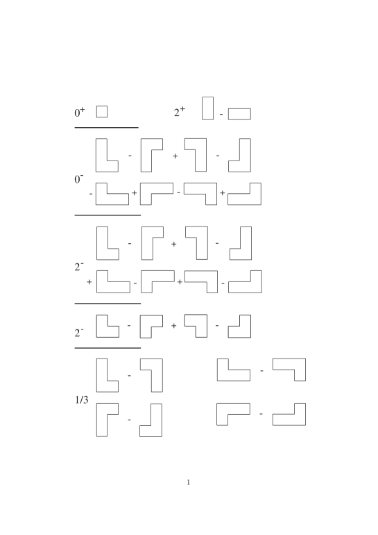
Figure 5: Some lattice realizations of the operators discussed in exercise 2. To clarify the role of the various symmetries, for the $2^{-}$ and 1/3 channels we have shown respectively two and four different realizations. For the $0^{+}$, $0^{-}$ and $2^{+}$ only the simplest possible realizations are shown.

On the cubic lattice the group of two dimensional rotations and reflections becomes the dihedral group $D_{4}$. This group is non abelian, has eight elements and five irreducible representations. Four of these are one-dimensional irreps, the last one has dimension two. The group structure is completely described by the table of characters [70] which we have reported in tab. 9 .

Table 9: Character table for the group $D_{4}$

	${\bf 1}$	$C_{4}^{2}$	$C_{4}(2)$	$C_{2}(2)$	$C_{2^{\prime}}(2)$
$A_{1}$	$1$	$1$	$1$	$1$	$1$
$A_{2}$	$1$	$1$	$1$	$-1$	$-1$
$B_{1}$	$1$	$1$	$-1$	$1$	$-1$
$B_{2}$	$1$	$1$	$-1$	$-1$	$1$
$E$	$2$	$-2$	$0$	$0$	$0$

In the top row of tab. 9 are listed the invariant classes of the group, and in the first column the irreducible representations. We followed the notations of [70] to label classes and representation (with the exception of the class containing the identity which we have denoted with ${\bf 1}$ instead of the usual $E$ to avoid confusion with the two-dimensional representation). The entries of the table allow to explicitly construct the various representations and hence also the lattice operators which we are looking for. The relationship of these operators with the various glueball states immediately follows from the group structure. In particular one can show that:

a] Only operators with angular momentum $J~{}(mod(4))$ can be constructed. This is a common feature of all cubic lattice regularizations. It means that glueball states which in the continuum have values of $J$ higher than 3 appear on the lattice as secondary states in the family of the corresponding $J~{}(mod(4))$ lattice operator.

b] The four one-dimensional irreps are in correspondence with the even $J$ states. More precisely:

$$0^{+}\to A_{1},\hskip 28.45274pt0^{-}\to A_{2},\hskip 28.45274pt2^{+}\to B_{1},\hskip 28.45274pt2^{-}\to B_{2}$$

This means that the discreteness of the lattice splits the degeneracy between $2^{+}$ and $2^{-}$ which we discussed above. The splitting between these two states gives us a rough estimates of relevance of the breaking of the full rotational group due to the lattice discretization. Precise Montecarlo data [83] have shown that in the scaling region this splitting is essentially zero within the errors, in agreement with our expectation that approaching the continuum limit the full continuum symmetries should be recovered. Notice however that this is a very non-trivial result since the operators associated to $2^{+}$ and $2^{-}$ on the lattice turn out to be very different.

c] All the odd parity states are grouped together in the two-dimensional irreducible representation $E$. This means that we cannot distinguish among them on the basis of the lattice symmetries. We can conventionally assume, say, that the $J=1$ states have a mass lower than the $J=3$ ones, and that the $J=3$ thus appear as secondaries in the $J=1$ family. In agreement with the above discussion, if the full rotational symmetry is recovered, we expect the states belonging to this family to be degenerate in parity and thus the lowest mass states, which are the ones that we can measure more precisely, to appear as a doublet. Also this prediction agrees with the data of [83].

The simplest lattice operators, constructed according to the character table, are shown in fig. 5.

A.3 Exercise 3: Character Expansion for the $SU(N)$ group.

In this exercise we shall give some basic informations on the character expansion for $SU(N)$ groups, and shall then expand, as an example the Wilson action in the character basis (for further details see Ref. [80]). Notice that, even if we deal in particular with the SU$(N)$ groups, most of the results that we shall discuss can hold for any Lie group $G$ and with minor modifications also for discrete groups.

The irreducible characters $\chi_{r}(U)$ are the traces of the irreducible representations (labelled by $r$) of the group. They form a complete orthonormal basis for the class functions on the group. A function $f(U)$ on the group is called a “class function” if it satisfies the relation:

$$f(U)=f(VUV^{\dagger})\hskip 56.9055pt\forall\,V\in{\rm SU}(N)~{}.$$ (E3.1)

In particular, the characters themselves are class functions. The pure gauge action, eq. (13), is a class function.

The following orthogonality relations between characters hold:

$$\int dU\,\chi_{r}(U)~{}\chi^{*}_{s}(U)=\delta_{r,s}~{},$$ (E3.2)

$$\sum_{r}d_{r}\chi_{r}(U~{}V^{\dagger})=\delta(U,V)~{},$$ (E3.3)

where $dU$ denotes the Haar measure (normalized to unity) on $SU(N)$ and $d_{r}$ denotes the dimension of the $r^{\rm th}$ representation.

Besides the above orthogonality relations there are two two other integration formulas of the characters which turn out to be very useful in the construction of SC expansions:

$$\int dU\,\chi_{r}(V_{1}U)~{}\chi_{s}(U^{\dagger}V_{2})=\delta_{r,s}\frac{\chi_{r}(V_{1}V_{2})}{d_{r}}~{};$$ (E3.4)

$$\int dU\,\chi_{r}(UV_{1}U^{\dagger}V_{2})=\frac{1}{d_{r}}\chi_{r}(V_{1})\chi_{r}(V_{2})~{}.$$ (E3.5)

Any class function can be expanded in the basis of the characters:

$$f(U)=\sum_{r}\chi_{r}(U)f_{r}~{},$$ (E3.6)

where the sum is over the set of all irreducible representations of the group, and the coefficients $f_{r}$ are given by

$$f_{r}\equiv\int dU\,\chi^{*}_{r}(U)f(U)~{}.$$ (E3.7)

Let us construct now the character expansion for the Wilson action.

The Boltzmann factor associated to each plaquette in the Wilson action is (see eq.(13)) :

$${\rm e}^{\frac{\beta}{N}{\rm Re}{\rm Tr}U_{\mu\nu}(n)}=\sum_{r}F_{r}(\beta)\chi_{r}(U_{\mu\nu}(n))~{},$$ (E3.8)

Notice that a factor 2 has been eliminated in the Boltzmann weight with respect to eq.(13) so as to avoid a double counting of the plaquettes. The coefficients $F_{r}$ are given by:

$$F_{r}(\beta)\equiv\int dU\,{\rm e}^{\frac{\beta}{N}{\rm Re}{\rm Tr}U}\chi^{*}_{r}(U)=\sum_{n=-\infty}^{\infty}{\rm det}\,I_{r_{j}-j+i+n}(\frac{\beta}{N})~{}.$$ (E3.9)

The $r_{j}$’s are a set of integers labelling the representation $r$ and they are constrained by: $r_{1}\geq\cdots\geq r_{N}=0$. The indices $1\leq i,j\leq N$ label the entries of the $N\times N$ matrix of which the determinant is taken and $I_{n}(\beta)$ denotes the modified Bessel function of order $n$.

As a consequence of the factor $d_{r}$ at the denominator in eq.s (E3.4, E3.5) the relevant coefficients in the character expansion (E3.8), namely the ones that will appear in the strong coupling expansions, are not the $F_{r}$ themselves, but the following normalized coefficients:

$$D_{r}(\beta)=\frac{F_{r}(\beta)}{d_{r}F_{0}(\beta)}~{}.$$ (E3.10)

Let us see in more detail two examples: the case of $SU(2)$ and the large $N$ limit.

Character expansion for $SU(2)$ We can parameterize the most general matrix $U$ belonging to $SU(2)$ by using the Pauli $\sigma$ matrices.

$$U=cos(\theta/2)+i\vec{\sigma}\vec{n}sin(\theta/2)~{}~{}~{}~{}~{}~{}~{}~{}~{}~{}(0\leq\theta<4\pi)~{}~{},$$ (E3.11)

where $\vec{n}$ is a three dimensional normalized vector.

The normalized Haar measure is in this case

$$DU=\sin^{2}(\theta/2)\frac{d\theta}{2\pi}\frac{d^{2}\vec{n}}{4\pi}~{}~{}~{}~{}.$$ (E3.12)

The irreducible representations are labeled by the angular momentum $j=0,\frac{1}{2},1,\cdots$ and have dimension $d_{j}=2j+1$.

The character of the $j^{th}$ irreducible representation is:

$$\chi_{j}(U)=\frac{\sin(j+\frac{1}{2})\theta}{\sin(\theta/2)}$$ (E3.13)

The Wilson action is in this case

$$exp\{\frac{1}{2}\beta\chi_{\frac{1}{2}}(U)\}\equiv exp\{\beta\cos(\theta/2)\}$$ (E3.14)

where $U$ is the plaquette variable.

If we insert eq.(E3.13) and (E3.14) in eq.(E3.9) we immediately recognize one of the integral representations of the modified Bessel functions.

Thus the expansion of the Wilson action in the character basis is

$$exp\{\frac{1}{2}\beta\chi_{\frac{1}{2}}(U)\}=\sum_{j}2(2j+1)\frac{I_{2j+1}(\beta)}{\beta}\chi_{j}(U)$$ (E3.15)

From this one can immediately recover the expression for the normalized coefficients $D_{j}(\beta)$

$$D_{j}(\beta)=\frac{I_{2j+1}(\beta)}{I_{1}(\beta)}$$ (E3.16)

Character expansion in the large $N$ limit It is easy to see that in the large $N$ limit we find a finite value for the coefficients $D_{r}(\beta)$ only if we simultaneously take the $\beta\to\infty$ limit while keeping the $\beta/N$ ratio fixed (in agreement with the ’t Hooft prescription). In this limit the coefficients $F_{r}(\beta)$ turn out to have a very simple form. In particular in the region $\beta/N<1$ one finds:

$$F_{0}(\beta/N) \sim {\rm e}^{\left(\frac{\beta}{2}\right)^{2}}~{},$$

$$F_{f}(\beta/N) \sim \frac{\beta}{2}\,{\rm e}^{\left(\frac{\beta}{2}\right)^{2}}~{},$$

where the index $f$ denotes the fundamental representation (whose dimension is $N$). The above relations imply that in the large $N$ limit

$$D_{f}(\beta/N)=\frac{\beta}{2N}~{}.$$ (E3.17)

Similar simplified relations hold also for higher representations.

A.4 Exercise 4: Evaluate the first order of the strong coupling expansion of the Wilson loop in $YM$ theories.

Let us evaluate the first term in the strong coupling expansion the expectation value $\langle\chi_{f}(U_{c})\rangle$, where $U_{c}$ is the ordered product of gauge variables along a Wilson loop “C” of size $R\times T$ and $\chi_{f}$ denotes the character of the fundamental representation. Following eq.(28) the expectation value is defined as:

$$\langle\chi_{f}(U_{c})\rangle=\frac{\int\prod_{n,\mu}dU_{\mu}(n)\chi_{f}(U_{c})e^{-S_{W}}}{Z}$$ (E4.1)

The first step is to insert in eq.(E4.1) the character expansion of the Wilson action (see eq.(E3.8)). The first non vanishing term in the expansion is the one in which we keep for all the plaquettes inside the Wilson loop (along the cristallographic plane, which ensures that we are keeping the minimum number of terms) and only for them, exactly the term in the expansion proportional to the fundamental representation. See fig. (6). In this way for all the links inside the Wilson loop and along the border we exactly find integrals of the type of eq.(E3.4).

This allow to perform all the group integrations in the expectation value, link after link. Each plaquette inside the loop gives a contribution $F_{f}(\beta)$, they are exactly $RT$. Each integration over the links gives a factor $1/d_{f}$. Again these are $RT$ (one must take into account the fact that for each integration that we perform some of the remaining links join together and thus at the end the total number of link integrals is not $2RT$ but only $RT$). Finally we must keep into account the $Z$ factor at the denominator of the expectation value. The simplest way to do this is to reorganize the strong coupling expansion so as to factorize also in front of the numerator the same factor $Z$. This simply amounts to normalize the coefficients of the expansion dividing them by $F_{0}(\beta)$. Collecting everything together we find

$$\langle\chi_{f}(U_{c})\rangle\sim\left(\frac{F_{f}(\beta)}{d_{f}F_{0}(\beta)}\right)^{RT}\equiv D_{f}(\beta)^{RT}~{}~{}~{}.$$ (E4.2)

This explains, by the way, why we introduced the normalized coefficients $D_{r}(\beta)$ in eq.(E3.10).

By using the definition of $\sigma$ (see eq.(43)) we immediately obtain from (E4.2)

$$\sigma=-\log D_{f}(\beta)$$ (E4.3)

Figure 6: Strong coupling expansion for the Wilson loop.

A.5 Exercise 5: Evaluate the first order of the strong coupling expansion of the lowest glueball mass in $YM$ theories.

The solution of this exercise goes along the same lines of the one on the Wilson loop. The only non trivial point is that we must find the surface of minimal area bordered by the two plaquettes. If we are interested in the lowest glueball state (i.e. the $0^{++}$ state) we know (see sect. 3.1.2) that it is enough to study the connected correlator of two elementary spacelike plaquettes (in the fundamental representation) located at two values of the time coordinate $t_{1}$ and $t_{2}$ in the limit in which $t\equiv|t_{2}-t_{1}|\to\infty$. In this limit the connected correlator decays exponentially, i.e.

$$\langle\chi_{f}(U_{ij}({\bf x},t_{1}))~{}\chi_{f}(U_{ij}({\bf x},t_{2}))\rangle\sim e^{-Mt}$$ (E5.1)

where $(U_{ij}({\bf x},t_{1}))$ is the plaquette (with spacelike indices $(i,j)$) located in the point $({\bf x},t_{1})$ of the lattice, and $M$ is the mass of the lowest glueball. It is easy to see that with this geometry the minimal surface connecting the two plaquettes is a long tube made of $4t$ plaquettes. Hence at the first order in the strong coupling expansion we have

$$\langle\chi_{f}(U_{ij}({\bf x},t_{1}))~{}\chi_{f}(U_{ij}({\bf x},t_{2}))\rangle\sim D_{f}(\beta)^{4t}$$ (E5.2)

from which we immediately see that

$$M(0^{++})=-4\log(D_{f}(\beta))$$ (E5.3)

A.6 Exercise 6: The effective string contribution to a rectangular Wilson loop.

In this exercise we construct the effective string theory contribution for a Wilson loop in the infrared limit, assuming a simple Nambu-Goto action for the string. As discussed in sect. 3.5 the Nambu-Goto action reduces in this limit to the theory of $d-2$ free massless scalar fields. In this exercise we shall compute the corresponding partition function $Z_{q}(R,T)$ which appears in eq. (52) following the discussion of ref. [71] (and references therein).

The Nambu string action is given by the area of the world–sheet:

$$S=\sigma\int_{0}^{T}d\tau\int_{0}^{R}d\varsigma\sqrt{g}\ \ ,$$ (E6.1)

where $g$ is the determinant of the two–dimensional metric induced on the world–sheet by the embedding in $R^{d}$:

$$g=\det(g_{\alpha\beta}) = \det\ \partial_{\alpha}X^{\mu}\partial_{\beta}X^{\mu}\ \ .$$

$$(\alpha,\beta=\tau,\varsigma,\ \mu=1,\dots,d)$$

and $\sigma$ is the string tension.

The reparametrization and Weyl invariances of the action (E6.1) require a gauge choice for quantization. We choose the ”physical gauge”

$$X^{1} = \tau$$

$$X^{2} = \varsigma$$ (E6.3)

so that $g$ is expressed as a function of the transverse degrees of freedom only:

$$g = 1+\partial_{\tau}X^{i}\partial_{\tau}X^{i}+\partial_{\varsigma}X^{i}\partial_{\varsigma}X^{i}$$

$$\ \ \ +\partial_{\tau}X^{i}\partial_{\tau}X^{i}\partial_{\varsigma}X^{j}\partial_{\varsigma}X^{j}-(\partial_{\tau}X^{i}\partial_{\varsigma}X^{i})^{2}$$

$$\ \ \ \ (i=3,\dots,d)~{}.$$

The fields $X^{i}(\tau,\varsigma)$ satisfy Dirichlet boundary conditions on $M$:

$$X^{i}(0,\varsigma)=X^{i}(T,\varsigma)=X^{i}(\tau,0)=X^{i}(\tau,R)=0\ \ .$$ (E6.5)

Due to the Weyl anomaly this gauge choice can be performed at the quantum level only in the critical dimension $d=26$. However, the effect of the anomaly is known to disappear at large distances [72], which is the region we are interested in.

Expanding the square root in Eq. (E6.1) we obtain, discarding terms of order $X^{4}$ and higher

$$S = \sigma RT+\frac{\sigma}{2}\int d^{2}\xi X^{i}(-\partial^{2})X^{i}$$ (E6.6)

$$\partial^{2} = \partial_{\tau}^{2}+\partial_{\varsigma}^{2}~{}.$$ (E6.7)

It is easy to see that this expansion of the action corresponds, for the partition function, to an expansion in powers of $(\sigma RT)^{-1}$. Therefore the action (E6.6) describes the infrared limit of the model defined by Eq. (E6.1), and will be relevant to the physics of large Wilson loops. The contribution of the fluctuations of the flux–tube to the Wilson loop expectation value in the infrared limit will be the partition function of our CFT, given by

$$Z_{q}(R,T)\propto\left[\det(-\partial^{2})\right]^{-\frac{d-2}{2}}~{}.$$ (E6.8)

The determinant must be evaluated with Dirichlet boundary conditions.

The spectrum of $-\partial^{2}$ with Dirichlet boundary conditions is given by the eigenvalues

$$\lambda_{mn}=\pi^{2}\left(\frac{m^{2}}{T^{2}}+\frac{n^{2}}{R^{2}}\right)$$ (E6.9)

corresponding to the normalized eigenfunctions

$$\psi_{mn}(\xi)=\frac{2}{\sqrt{RT}}\sin\frac{m\pi\tau}{T}\sin\frac{n\pi\varsigma}{R}~{}.$$ (E6.10)

The determinant appearing in Eq. (E6.8) can be regularized with the $\zeta$-function technique: defining

$$\zeta_{-\partial^{2}}(s)\equiv\sum_{mn=1}^{\infty}\lambda_{mn}^{-s}\ \,$$ (E6.11)

the regularized determinant is defined through the analytic continuation of $\zeta_{-\partial^{2}}^{\prime}(s)$ to $s=0$:

$$\det(-\partial^{2})=\exp\left[-\zeta_{-\partial^{2}}^{\prime}(0)\right]\ \ .$$ (E6.12)

The series in Eq. (E6.11) can be transformed, using the Poisson summation formula, to read

$$\zeta_{-\partial^{2}}(s)=-\frac{1}{2}\left(\frac{R^{2}}{\pi^{2}}\right)^{s}\zeta_{R}(2s)+\frac{\sqrt{\pi}Im\tau\Gamma(s-1/2)}{2\Gamma(s)}\left(\frac{R^{2}}{\pi^{2}}\right)^{s}\zeta_{R}(2s-1)$$

$$\ \ \ +\frac{2\sqrt{\pi}}{\Gamma(s)}\left(\frac{T^{2}}{\pi^{2}}\right)^{s}\sum_{n=1}^{\infty}\sum_{p=1}^{\infty}\left(\frac{\pi p}{nIm\tau}\right)^{s-1/2}K_{s-1/2}(2\pi pnIm\tau)$$ (E6.13)

where $\tau=iT/R$, $\zeta_{R}(s)$ is the Riemann $\zeta$ function and $K_{\nu}(x)$ is a modified Bessel function. The derivative $\zeta_{-\partial^{2}}^{\prime}(s)$ can be analytically continued to $s=0$ where it is given by

$$\zeta_{-\partial^{2}}^{\prime}(0)=\log(\sqrt{2R})-\frac{i\pi\tau}{12}-\sum_{n=1}^{\infty}\log(1-q^{n})$$ (E6.14)

where we have defined

$$q\equiv e^{2\pi i\tau}~{}.$$ (E6.15)

Introducing the Dedekind $\eta$-function

$$\eta(\tau)=q^{1/24}\Pi_{n=1}^{\infty}(1-q^{n})$$ (E6.16)

we obtain finally

$$\det(-\partial^{2})=\exp[-\zeta_{-\partial^{2}}^{\prime}(0)]=\frac{\eta(\tau)}{\sqrt{2R}}$$ (E6.17)

and

$$Z_{q}(R,T)\propto\left[\frac{\eta(\tau)}{\sqrt{R}}\right]^{-\frac{d-2}{2}}~{}.$$ (E6.18)

Substituting in Eq. (52) we obtain [71]

$$<W(R,T)>=e^{-\sigma RT+p(R+T)+k}\left[\frac{\eta(\tau)}{\sqrt{R}}\right]^{-\frac{d-2}{2}}~{}.$$ (E6.19)

Notice, as a concluding remark, that it is clear from the above discussion that the Nambu-Goto action that we studied in this exercise is only an instance of a large class of bosonic effective string models which reduce to the CFT studied in this exercise in the infrared limit. This is one of the possible explanations for the “string universality” discussed in sect. 3.5.3.

References

- [1] H. B. Nielsen and P. Olesen, “Vortex Line Models For Dual Strings,” Nucl. Phys. B61 (1973) 45.
- [2] G. ’t Hooft, “A Two-Dimensional Model For Mesons,” Nucl. Phys. B75 (1974) 461.
- [3] K. G. Wilson, “Confinement Of Quarks,” Phys. Rev. D10 (1974) 2445.
- [4] A. M. Polyakov, “String Representations And Hidden Symmetries For Gauge Fields,” Phys. Lett. B82 (1979) 247. A. M. Polyakov, “Gauge Fields As Rings Of Glue,” Nucl. Phys. B164 (1980) 171.
- [5] J. Gervais and A. Neveu, “The Quantum Dual String Wave Functional In Yang-Mills Theories,” Phys. Lett. B80 (1979) 255.
- [6] Y. Nambu, “QCD And The String Model,” Phys. Lett. B80 (1979) 372.
- [7] T. Eguchi and H. Kawai, “Reduction Of Dynamical Degrees Of Freedom In The Large N Gauge Theory,” Phys. Rev. Lett. 48 (1982) 1063.
- [8] J. Maldacena, “The Large Limit of Superconformal Field Theories and Supergravity,” Adv. Theor. Math. Phys. 2 (1998) 231. hep-th/9711200.
- [9] E. Witten, “Anti-de Sitter Space, Thermal Phase Transition, And Confinement In Gauge Theories” Adv.Theor.Math.Phys. 2, 253 (1998), hep-th/9803131.
- [10] K. Osterwalder and R. Schrader, “Axioms For Euclidean Green’s Functions,” Commun. Math. Phys. 31 (1973) 83. K. Osterwalder and R. Schrader, “Axioms For Euclidean Green’s Functions. 2,” Commun. Math. Phys. 42 (1975) 281.
- [11] R. Johnson and M. Teper, “Distinguishing J = 4 from J = 0 on a cubic lattice,” Nucl. Phys. Proc. Suppl. 73 (1999) 267 hep-lat/9808012.
- [12] H. Arisue and K. Tabata, “Strong coupling expansion of mass gap for Z(2) lattice gauge theory in three dimensions,” Phys. Lett. B322 (1994) 224.
- [13] V. Agostini, G. Carlino, M. Caselle and M. Hasenbusch, “The spectrum of the 2+1-dimensional gauge Ising model,” Nucl. Phys. B484 (1997) 331 hep-lat/9607029. M. Caselle and M. Hasenbusch, “Universal amplitude ratios in the 3D Ising model,” J. Phys. A A30 (1997) 4963 hep-lat/9701007.
- [14] E. Witten, Proc. Nato Adv. Study Institute on Recent Developments in Gauge Theories (Plenum Press, N.Y. 1980).
- [15] Y.M. Makeenko and A.A. Migdal, “Exact Equation for The Loop Average in Multicolor QCD,” Phys. Lett. 88B, 135 (1979); Y. Makeenko and A.A. Migdal, “Quantum Chromodynamics as Dynamics of Loops,” Nucl. Phys. B188, 269 (1981).
- [16] A.A. Migdal, “Loop Equations and Expansion,” Phys. Rept. 102, 199 (1984).
- [17] V.A. Kazakov and I.K. Kostov, “Nonlinear Strings in Two-Dimensional Gauge Theory,” Nucl. Phys. B176, 321 (1980)
- [18] S.M. Das, Rev. of Modern Physics 59 (1987) 235.
- [19] M. Billó, M. Caselle, A. D’Adda and S. Panzeri, “Finite temperature lattice QCD in the large N limit,” Int. J. Mod. Phys. A12 (1997) 1783 hep-th/9610144.
- [20] A. Hasenfratz, E. Hasenfratz and P. Hasenfratz, “Generalized Roughening Transition And Its Effect On The String Tension, ” Nucl. Phys. B180 (1981) 353. C. Itzykson, M. E. Peskin and J. B. Zuber, “Roughening Of Wilson’s Surface,” Phys. Lett. B95 (1980) 259.
- [21] M. Lüscher, K. Symanzik and P. Weisz, “Anomalies Of The Free Loop Wave Equation In The Wkb Approximation,” Nucl. Phys. B173 (1980) 365. M. Lüscher, “Symmetry Breaking Aspects Of The Roughening Transition In Gauge Theories, ” Nucl. Phys. B180 (1981) 317.
- [22] M. Caselle, R. Fiore, F. Gliozzi, M. Hasenbusch, K. Pinn and S. Vinti, “Rough interfaces beyond the Gaussian approximation,” Nucl. Phys. B432 (1994) 590 hep-lat/9407002.
- [23] M. Lüscher, G. Munster and P. Weisz, “How Thick Are Chromoelectric Flux Tubes?,” Nucl. Phys. B180 (1981) 1.
- [24] M. Caselle, F. Gliozzi, U. Magnea and S. Vinti, “Width of Long Colour Flux Tubes in Lattice Gauge Systems,” Nucl. Phys. B460 (1996) 397 hep-lat/9510019.
- [25] M. Caselle, R. Fiore, F. Gliozzi, M. Hasenbusch and P. Provero, “String effects in the Wilson loop: A high precision numerical test,” Nucl. Phys. B486 (1997) 245 hep-lat/9609041.
- [26] C. Bachas, “Convexity of the Quarkonium Potential,” Phys. Rev. D33 (1986) 2723.
- [27] G. S. Bali and K. Schilling, “Static quark-antiquark potential: Scaling behaviour and finite size effects in SU(3) LGT,” Phys. Rev. D46, 2636 (1992).
- [28] G. S. Bali, K. Schilling, and A. Wachter, “Complete corrections to the static interquark potential from gauge theory,” Phys. Rev. D56, 2566 (1997), hep-lat/9703019.
- [29] M. Caselle, R. Fiore, F. Gliozzi, P. Guaita and S. Vinti, “On the behavior of spatial Wilson loops in the high temperature phase of LGT,” Nucl. Phys. B422 (1994) 397 hep-lat/9312056. M. Caselle and A. D’Adda, “The Spatial string tension in high temperature lattice gauge theories,” Nucl. Phys. B427 (1994) 273 hep-lat/9403027.
- [30] C. J. Morningstar and M. Peardon, “The glueball spectrum from an anisotropic lattice study,” Phys. Rev. D60, 034509 (1999), hep-lat/9901004.
- [31] E. Witten, “Anti-de Sitter space and holography,” Adv. Theor. Math. Phys. 2 (1998) 253 [hep-th/9802150].
- [32] S. S. Gubser, I. R. Klebanov and A. M. Polyakov, “Gauge theory correlators from non-critical string theory,” Phys. Lett. B428 (1998) 105 [hep-th/9802109].
- [33] A. M. Polyakov, “String theory and quark confinement,” Nucl. Phys. Proc. Suppl. 68 (1998) 1 [hep-th/9711002].
- [34] A. M. Polyakov, “Confining strings,” Nucl. Phys. B486 (1997) 23 [hep-th/9607049].
- [35] I. R. Klebanov, “World-volume approach to absorption by non-dilatonic branes,” Nucl. Phys. B496 (1997) 231 [hep-th/9702076].
- [36] S. S. Gubser, I. R. Klebanov and A. A. Tseytlin, “String theory and classical absorption by three-branes,” Nucl. Phys. B499 (1997) 217 [hep-th/9703040].
- [37] M. Douglas, J. Polchinski and A. Strominger, “Probing five-dimensional black holes with D-branes,” JHEP 9712 (1997) 003 [hep-th/9703031].
- [38] I. Montvay, “Simulation of QCD and other similar theories,” hep-lat/9909020.
- [39] C. Csaki, H. Ooguri, Y. Oz, J. Terning “Glueball Mass Spectrum From Supergravity” JHEP 9901, 017 (1999), hep-th/9806201,
- [40] R.de Mello Koch, A. Jevicki, M. Mihailescu, J. P. Nunes, “Evaluation of glueball masses from supergravity”, Phys.Rev. D58 (1998) 105009, hep-th/9806125
- [41] M.Zyskin “A note on the glueball mass spectrum”, Phys. Lett. B439 (1998) 373, hep-th/9806128.
- [42] N.R.Constable and R.C Myers, “Spin-two glueballs, positive energy theorems and the AdS/CFT correspondence”, JHEP 9910 (1999) 037, hep-th/9908175.
- [43] R.Brower, S.D.Mathur and C.-I Tan, “Discrete spectrum of the graviton in the black hole background”, hep-th/9908196.
- [44] H. Ooguri, H.Robin, J. Tannenhauser, “Glueballs and their Kaluza-Klein cousins” Phys.Lett. B437, 77(1998), hep-th/9806171.
- [45] J. G. Russo, “New Compactifications of Supergravities and Large N QCD” Nucl.Phys. B543, 183 (1999), hep-th/9808117.
- [46] C. Csaki, Y. Oz, J. Russo, J. Terning, “Large N QCD from Rotating Branes” Phys.Rev. D59, 065012 (1999), hep-th/9810186.
- [47] J.G. Russo, K. Sfetsos, “Rotating D3-branes and QCD in three dimensions” Adv. Theor. Math. Phys. 3, 131 (1999), hep-th/9901056.
- [48] C. Csaki, J. Russo, K. Sfetsos, J.Terning, “Supergravity Models for 3+1 Dimensional QCD” Phys.Rev. D60, 044001 (1999), hep-th/9902067.
- [49] K. Suzuki, “ systems and ” hep-th/0001057.
- [50] J.A. Minahan, “Glueball mass spectra and other issues for supergravity duals of QCD models” JHEP 9901, 020 (1999), hep-th/9811156.
- [51] J. Maldacena, “Wilson loops in large N field theories” Phys.Rev.Lett. 80, 4859 (1998), hep-th/9803002.
- [52] S.J. Rey, J. Yee, “Macroscopic strings as heavy quarks in large N gauge theory and Anti-de Sitter supergravity” hep-th/9803001;
- [53] A. Brandhuber, N. Itzhaki, J. Sonnenschein, S. Yankielowicz, “Wilson loops, confinement, and phase transitions in large N gauge theories from supergravity” JHEP 9806, 001 (1998), hep-th/9803263.
- [54] S.J. Rey, S. Theisen, J. Yee, “Wilson-Polyakov loop finite temperature in large N gauge theory and Anti-de Sitter supergravity” Nucl.Phys. B527, 171 (1998), hep-th/9803135.
- [55] Nadav Drukker, David J. Gross, Hirosi Ooguri, “Wilson Loops and Minimal Surfaces”, Phys. Rev. D60 (1999) 125006, hep-th/9904191
- [56] Nadav Drukker, David J. Gross, Arkady A. Tseytlin, “Green-Schwarz string in : Semiclassical partition function,” hep-th/0001204
- [57] J. Greensite, P. Olesen, “Remarks on the Heavy Quark Potential in the Supergravity Approach” JHEP 9808 (1998) 009, hep-th/9806235
- [58] P. Olesen, “Some speculations on the gauge coupling in the ADS/CFT approach” JHEP 9904 (1999) 001, hep-th/9904034
- [59] J. Greensite, P. Olesen, “Worldsheet Fluctuations and the Heavy Quark Potential in the AdS/CFT Approach”, JHEP 9904 (1999) 001, hep-th/9901057
- [60] S. Forste, D. Ghoshal, S. Theisen, “Stringy Corrections to the Wilson Loop in N=4 Super Yang-Mills Theory”, JHEP 9908 (1999) 013, hep-th/9903042.
- [61] Y. Kinar, E. Schreiber, J. Sonnenschein and N. Weiss, “Quantum fluctuations of Wilson loops from string models”, hep-th/9911123.
- [62] S. Naik, “Improved heavy quark potential at finite temperature from anti-de Sitter supergravity”, Phys. Lett. B464 (1999) 73, hep-th/9904147.
- [63] H.Dorn and V.D.Pershin, “Concavity of the potential in the super Yang-Mills gauge theory and AdS/CFT duality” hep-th/9906073
- [64] K. Zarembo, “Wilson loop correlator in the AdS/CFT correspondence,” Phys. Lett. B459 (1999) 527 hep-th/9904149.
- [65] J. Erickson, G. W. Semenoff and K. Zarembo, “BPS vs. non-BPS Wilson loops in N = 4 supersymmetric Yang-Mills theory, ” Phys. Lett. B466 (1999) 239 hep-th/9906211.
- [66] J. Sonnenschein and A. Loewy, “On the supergravity evaluation of wilson loops correlators in confining theories”, hep-th/9911172.
- [67] M. Caselle, F. Gliozzi and U. Magnea, “Fluid interfaces in the 3-d Ising model as a dilute gas of handles,” Physica A215 (1995) 21.
- [68] A.M. Polyakov, “Gauge Fields and Strings,” Harwood (1987) 301 p. (Contemporary Concepts in Physics, 3).
- [69] D.J. Gross, H. Ooguri, “Aspects of large N gauge theory dynamics as seen by string theory” Phys.Rev. D58, 106002 (1998), hep-th/9805129.
- [70] M. Hamermesh, Group Theory and its Application to Physical Problems, Reading Mass.: Addison-Wesley, 1962
- [71] J. Ambjorn, P. Olesen and C. Peterson, “Three-Dimensional Lattice Gauge Theory And Strings,” Nucl. Phys. B244 (1984) 262.
- [72] P. Olesen, “Strings And QCD,” Phys. Lett. B160 (1985) 144. Books and Reviews on L.G.T.
- [73] C. Rebbi, Lattice Gauge Theories and Montecarlo Simulations, World Scientific 1983.
- [74] M. Creutz, Quarks, Gluons, and Lattices, Cambridge University Press, 1983.
- [75] Quantum Fields on the Computer, Ed. M. Creutz, World Scientific, 1992.
- [76] I. Montvay and G. Münster, Quantum Fields on a Lattice, Cambridge University Press, 1994.
- [77] C. Itzykson and J.-M. Drouffe, Statistical Field Theory, Cambridge University Press, 1989. (In particular chapters 6,7 and 8 are devoted to L.G.T.)
- [78] J. B. Kogut, “An Introduction To Lattice Gauge Theory And Spin Systems,” Rev. Mod. Phys. 51 (1979) 659.
- [79] J. B. Kogut, “A Review Of The Lattice Gauge Theory Approach To Quantum Chromodynamics, ” Rev. Mod. Phys. 55 (1983) 775.
- [80] J.M. Drouffe and J.B. Zuber, “Strong Coupling and Mean Field Methods in Lattice Gauge Theories,” Phys. Rep. 102(1983) 1.
- [81] R. Gupta, Introduction to lattice QCD. Les Houches lectures (1997 Summer School), hep-lat/9807028
- [82] M. Lüscher Advanced Lattice QCD Les Houches lectures (1997 Summer School), hep-lat/9802029
- [83] M. J. Teper, SU(N) gauge theories in (2+1) dimensions Phys. Rev. D59 (1999) 014512 hep-lat/9804008.
- [84] M. J. Teper, Glueball masses and other physical properties of SU(N) gauge theories in D = 3+1: A review of lattice results for theorists. hep-th/9812187.
- [85] G. S. Bali, “QCD forces and heavy quark bound states,” hep-ph/0001312
- [86] LATTICE93 Nucl. Phys. (Proc. Suppl.) B34 (1994); LATTICE94 Nucl. Phys. (Proc. Suppl.) B42 (1995); LATTICE95 Nucl. Phys. (Proc. Suppl.) B47 (1996); LATTICE96 Nucl. Phys. (Proc. Suppl.) B53 (1997); LATTICE97 Nucl. Phys. (Proc. Suppl.) B63 (1998); LATTICE98 Nucl. Phys. (Proc. Suppl.) B73 (1999). Reviews on the AdS/CFT correspondence.
- [87] P. Di Vecchia, “Large N gauge theories and AdS/CFT correspondence”, hep-th/9908148.
- [88] O.Aharony, S.S.Gubser, J.Maldacena, H.Ooguri and Y.Oz, “Large N field theories, string theory and gravity”, hep-th/9905111.