TAUP-2623-2000

In these lectures we describe the attempt to extract the expectation values of Wilson loops from the string/gauge correspondence. We start with the original calculation in $AdS_{5}\times S^{5}$. It is then extended to the non-conformal background of $D_{p}$ in the near horizon limit. We discuss the computation at finite temperature. Supergravity models that admit confinement in 3d and 4d are described. A theorem that determines the classical values of loops associated with a generalized background is derived. In particular we determine sufficient conditions for confining behavior. We then apply the theorem to various string models including type 0 ones. We describe an attempt to go beyond the classical string picture by incorporating quadratic quantum fluctuations. In particular we address the BPS configuration of a single quark, the supersymmetric determinant of $AdS_{5}\times S^{5}$  and a setup that corresponds to a confining gauge theory. We determine the form of the Wilson loop for actions that include non trivial $B_{\mu\nu}$ field. The issue of an exact determination of the value of the stringy Wilson loop is discussed. We end with a brief review of the baryons from the string/gauge correspondence

Lectures presented in the “Advanced School on Supersymmetry in the theories of fields, strings and branes” Santiago de Compostela-99.

1 Introduction

The idea to describe the Wilson loop of QCD in terms of a string partition function dates back to the early Eighties. For instance, a landmark paper in this direction [1] showed that the potential of quark anti-quark separated at a distance $L$ acquires a $-{c\over L}$ correction term ($c$ is a positive universal constant independent of the coupling) due to quantum fluctuations of a Nambu–Goto (NG) like action. An exact expression of the partition function of the NG action was derived in the large $d$ limit [2], where $d$ is the space-time dimension. The result, when translated to the quark anti-quark potential, took the following form $E(L)\sim{L\over\alpha^{\prime}}\sqrt{1-{2c\over L^{2}/\alpha^{\prime}}}$. Thus, by expanding it for small ${2c\over L^{2}/\alpha^{\prime}}$, one finds the linear confinement potential as well as the so called Lüscher term. It was later realized that in fact this expression is identical to the energy of the tachyonic mode of the bosonic string in flat spacetime with Dirichlet boundary conditions at $\pm L/2$ [3].

Recently there has been a Renaissance of the idea of a stringy description of the Wilson loop in the framework of Maldacena’s correspondence between large $N$ gauge theories and string theory [4, 5, 6, 7]. Technically, the main difference between the ”old” calculations and the modern ones is the fact that the spacetime background is no longer flat but rather curved and it includes additional “relevant” dimensions like the $AdS_{5}\times S^{5}$or certain deformation of it. Conceptually, the modern gauge/string duality gave the stringy description a more solid basis. The duality incorporate recipes of extracting physical properties of the boundary theory like correlation functions and others from the dual string theory. The Wilson loop falls into this category of physical gauge invariant properties that can be read from the string picture.

The first ”modern” computation [8, 9] was a classical calculation based on the $AdS_{5}\times S^{5}$metric which corresponds to the ${\cal N}=4$ supersymmetric theory. The geometrical shape of the loop was taken to be that of a infinite strip. It was then generalized to the circle [10] and to closed loops with cusps [11]. The latter paper further analyzed carefully the correspondence between the area of the string configuration and the Wilson loop as well as the contribution from the adjoint scalars to the expectation of the loop[14]

To make contact with non-supersymmetric gauge dynamics one makes use of Witten’s idea [12] of putting the Euclidean time direction on a circle with anti-periodic boundary conditions. This recipe was utilized to determine the behavior of the potential for the ${\cal N}=4$ theory at finite temperature [15, 13] as well as 3d pure YM theory [16] which is the limit of the former at infinite temperature. Later, a similar procedure was invoked to compute Wilson loops related to 4d YM theory, ‘t Hooft loops [16, 17] and the quark anti-quark potential in MQCD[18] and in Polyakov’s type 0 model [20, 21]. A unified scheme for all these models and variety of others was analyzed in [19]. A theorem that determines the leading and next to leading behavior of the classical potential associated with this unified setup was proven and applied to several models. In particular a corollary of this theorem states the sufficient conditions for the potential to have a confining nature.

Another map between string models and non-supersymmetric gauge theories is based on the correspondence with type 0 string theories[21]. It was argued that the RR tachyon interaction shifts $m^{2}$ of the tachyons to positive values. Area law Wilson loop characterizes the IR regime whereas in the UV asymptotically free-like behavior was detected[22, 23].

The baryonic configuration is another gauge invariant quantity that was identified in the string picture. First the baryonic vertex was idntified[26], then it was shown that the stringy baryons are stable[27] and finally they were related to exact solutions of the BPS equations[28, 29]

The issue of the quantum fluctuations and the detection of a Lüscher term was raised again in the modern framework in [31]. It was noticed there that a more accurate evaluation of the classical result [19] did not have the form of a Lüscher term. This is, of course, what one should have anticipated, since after all the origin of the Lüscher term [1] is the quantum fluctuations of the NG like string. The determinant associated with the bosonic quantum fluctuations of the pure YM setup was addressed in [31]. It was shown there that the system is approximately described by six operators that correspond to massless bosons in flat spacetime and two additional massive modes. The fermionic determinant was not computed in this paper. However, the authors raised the possibility that the latter will be of the form of massless fermions and hence there might be a violation of the concavity behavior of gauge potentials [52, 33].In [34] it was argued that in fact the fermionic operators are massive ones and thus the bosonic determinant dominates and there is an attractive interaction after all. The impact of the quantum fluctuations for the case of the $AdS_{5}\times S^{5}$case was discussed in [51, Naik]. Using the GS action [37, 38, 39, 48] with a particular $\kappa$ symmetry fixing, it was observed that the corresponding quantum Wilson loop suffers from UV logarithmic divergences. It was argued that by renormalizing the mass of the quarks one can remove the divergence.

The computations of Wilson loops in 3d and 4d pure YM theory can be confronted with the results found in lattice calculations. In particular, the main question is whether the correction to the linear potential in the form of a Lüscher term can be detected in lattice simulations. According to [41] there is some numerical evidence for a Lüscher term associated with a bosonic string, however the results are not precise enough to be convincing. Obviously,the ultimate dream is compatibility with heavy meson phenomenology. The topics discussed in these lectures were addressed in varius other publications[35]

The starting point of these lectures is the original determination of the Wilson loop[8] of the ${\cal N}=4$ SYM theory from the classical supargravity effective action of the type $II_{B}$ string theory on the $AdS_{5}\times S^{5}$background. We then extend in section 2 this calculation also to the generalized correspondence between non-conformal SYM theory with 16 supersymmetries in $d+1$ dimensions and the supergravity solution associated with $D_{d}$ branes in the the near horizon. For that purpose we first briefly describe this correspondence and then calculate the action of a static NG string in those backgrounds. In section 3 we analyze the behavior of the Wilson loop at finite temperature using a near extremal supergravity solution. It is shown that there is a critical separation length ( or critical temperature) above which the quark anti-quark are fully screened. Section 4 is devoted to the supergravity background which corresponds to pure YM theory in three and (four) dimensions, or to be more precise the limit of $T\rightarrow\infty$ of the maximal SYM theory in four ( five) dimensions. The set up is described, area law behavior of the Wilson loop is found as well as a screening behavior of a monopole anti-monopole pair via the ’t Hooft loop. A generalized Nambu Goto action for curved backgrounds with metric that depends on one coordinate is written down in section 5. A theorem that determines the leading and next to leading behavior of the Wilson loop associated with those scenarios is derived. A corolarry of that theorem determines necessary conditions for having an area law behavior. We then present a table where a list of models are analyzed using the results of the theorem. Other string models which can be analyzed using the tools that follow from the theorem are the various type zero models. In section 6 we briefly describe the string/gauge correspondence for the non -supersymmetric cases associated with type 0 models and then present the calculations of the Wilson loops in the various energy scales. Section 7 is devoted to the impact of the string quadratic quantum fluctuations. We address the issues of gauge fixing, the general structure of the bosonic determinant, the fluctuations in flat space-time, general scaling relation, the fermionic determinant in flat space-time, the determinant of a single quark in $AdS_{5}\times S^{5}$and the Wilson loop for that background and finally the derivation of the Luscher term for the confining cases. Section 8 is devoted to a discussion about possible exact determination of the Wilson loop. In section 9 we briefly discuss the determination of the Wilson loops in background with a non trivial WZ term. Section 10 is devoted to the analysis of baryons from supergravity. The basic baryonic vertex is described and implemented for the case of ${\cal N}=4$ and for the more interesting confining models.

2 The Wilson loop of ${\cal N}=4$

The Wilson loop operator is

$$W({\cal C})={1\over N}Tr[Pe^{i\oint_{\cal C}A}]$$

where ${\cal C}$ is a closed loop in space-time.

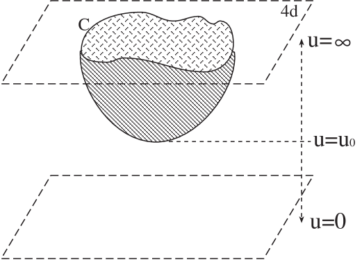
Figure 1: The basic setup of the Wilson loop

It is well known that one can extract the potential energy $E(L)$ of a system of external quark anti-quark from $<W({\cal C})>$ via

$$<W({\cal C})>=A(L)e^{-TE(L)}$$

for a loop which is an infinite strip ($T\rightarrow\infty$) (see fig. 2). Here is these lectures we restrict our attention only to loops with this type of shape. Loops of general shape, which are the natural objects in discussions of the loop equation, and in particular circular loops[10] and loops with cusps were analyzed in [11].

In fact in ${\cal N}=4$ the adjoint scalars can also “run” along the loop so the full Wilson loop is

$$W({\cal C})={1\over N}Tr[Pe^{i\oint_{{\cal C}}dsA_{\mu}\dot{\sigma}^{\mu}+\theta^{I}(s)X^{I}(\sigma)\sqrt{\dot{\sigma}^{2}}}]$$

Here we restrict ourselves only to the gauge fields. A way to introduce the infinitely heavy external quark pair is terms of $W$ bosons associated with the breaking of $U(N+1)\rightarrow U(N)$ where the expectation value of the Higgs field $\rightarrow\infty$

The natural candidate is

$$<W({\cal C})>\sim e^{-S}$$

where $S$ is the proper area of the string world-sheet which on the boundary of the $AdS_{5}$ is ${\cal C}$.

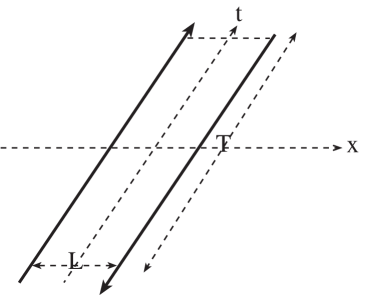
Figure 2: The Wilson loop setup for the $AdS_{5}\times S^{5}$

However, this includes the (infinite) mass of the W-bosons. The subtracted expression is

$$<W({\cal C})>\sim lim_{\Phi\rightarrow\infty}e^{-S_{\Phi}-l\Phi}$$

where $l$ is the length of the loop

In the framework of the correspondence between the $AdS_{5}\times S^{5}$supergravity theory and the large N, ${\cal}N=4$ super YM theory $S$ is given in terms of the Nambu-Goto action

$$S={1\over 2\pi{\alpha^{{}^{\prime}}}}\int d\tau d\sigma\sqrt{detG_{\mu\nu}\partial_{\alpha}X^{\mu}\partial_{\beta}X^{\nu}}$$

where $G_{\mu\nu}$ is the metric on the $AdS_{5}\times S^{5}$

$$ds^{2}=\alpha^{\prime}\left\{\frac{U^{2}}{R^{2}}[dt^{2}+dx_{i}^{2}]+R^{2}\frac{dU^{2}}{U^{2}}+R^{2}d\Omega_{5}^{2}\right\},$$

$$R^{2}=\sqrt{4\pi gN}$$

Notice that as expected the ${\alpha^{{}^{\prime}}}$ factors disappear.

Since we are interested in static configuration, it is natural to use the “static gauge” $\tau=t$ and $\sigma=x$ . In this gauge the action is

$$S = \frac{T}{2\pi}\int dx\sqrt{(\partial_{x}U)^{2}+(U^{4}/R^{4}}~{}~{}.$$ (1)

The “Hamiltonian” in the $x$ direction is a constant of motion.

$$\frac{U^{4}}{\sqrt{(\partial_{x}U)^{2}+(U^{4})/R^{4}}}=\mbox{const.}=R^{2}\sqrt{U_{0}^{4}},$$ (2)

This allows us to express $x$ as a function of $U$

$$x=\frac{R^{2}}{U_{0}}\int_{1}^{U/U_{0}}\frac{dy}{y^{2}\sqrt{(y^{4}-1)}}$$ (3)

where $U_{0}$ is determined by

$$L=2\frac{R^{2}}{U_{0}}\int_{1}^{\infty}\frac{dy}{y^{2}\sqrt{(y^{4}-1)}}=2\frac{R^{2}}{U_{0}}\frac{\sqrt{2}\pi^{3/2}}{\Gamma(1/4)^{2}}$$ (4)

The expression for the energy is regularized by integrating up to $U_{max}$ and renormalized by subtracting the mass of the $W$ boson $U_{max}/2\pi$ This renormalization is equivalent for the $AdS_{5}\times S^{5}$case to the use of the Legender transform of the energy advocated in [11]. The energy is given by

$$E=\frac{U_{0}}{\pi}\left\{\int_{1}^{\infty}\left(\frac{y^{2}}{\sqrt{y^{4}-1}}-1\right)-1\right\}.$$ (5)

so that the final expression for $E(L)$is

$$E=-{2\sqrt{2}\pi^{3/2}(4\pi g^{2}_{YM}N)^{1/2}\over\Gamma(1/4)^{4}}{1\over L}$$ (6)

The ${1\over L}$ dependence is dictated by conformal invariance since there is no scale in the problem. Notice however the non-trivial dependence $({g^{2}_{YM}N})^{1/2}$ which differs from the perturbative YM result $g^{2}_{YM}N$

3 Wilson loop for the non-conformal SYM theories with 16 Supersymmetries

A correspondence, which is a generalization of the Ads/CFT duality, between non-conformal boundary field theories in $p+1$ dimensions with 16 supersymmetries and the near horizon supergravity of $D_{p}$ branes was conjectured in [43]. The determination of the Wilson loop in those theories is thus a straightforward generalization of the computation performed for the $AdS_{5}\times S^{5}$background. We first briefly review the correspondence and then describe the result for the quark anti-quark energy.

3.1 A very brief review of the generalized correspondence

Let us examine now the generalization of the Ads/CFT duality to a correspondence between the SYM theory with 16 supersymetries in $p+1$ dimensions and the near horizon limit of the supergravity background of $N$ Dp-branes[43]. Consider a system of $N$ coincident extremal Dp-branes in the following limit [4]

$$g_{YM}^{2}=(2\pi)^{p-2}g_{s}{\alpha^{{}^{\prime}}}^{(p-3)/2}=\mbox{fixed},\;\;~{}~{}~{}~{}~{}{\alpha^{{}^{\prime}}}\rightarrow 0,~{}~{}~{}~{}~{}~{}U\equiv\frac{r}{{\alpha^{{}^{\prime}}}}=\mbox{fixed},$$ (7)

where $g_{s}=e^{\phi_{\infty}}$, and $g_{YM}$ is the coupling constant of the $p+1$ dimensional $U(N)$ SYM theory that lives on the $N$ Dp-branes. In the SYM picture $U$ corresponds to finite Higgs expectation value associated with a $U(N+1)\rightarrow U(N)\times U(1)$ symmetry breaking. The effective coupling of the SYM theory is $g_{eff}^{2}=g_{YM}^{2}NU^{p-3}$. Perturbation theory can be trusted in the region

$$g_{eff}\ll 1.$$ (8)

The type II supergravity solution describing $N$ coincident extremal Dp-branes is given by

$$ds^{2}=f_{p}^{-1/2}(-dt^{2}+dx_{1}^{2}+...+dx_{p}^{2})+f_{p}^{1/2}(dx_{p+1}^{2}+...+dx_{9}^{2}),$$

$$e^{-2(\phi-\phi_{\infty})}=f_{p}^{(p-3)/2},$$ (9)

$$A_{0...p}=-\frac{1}{2}(f_{p}^{-1}-1),$$

where $f_{p}$ is a harmonic function of the transverse coordinates $x_{p+1},...,x_{9}$

$$\alpha^{\prime 2}f_{p}=\alpha^{\prime 2}+\frac{d_{p}g^{2}_{YM}N}{U^{7-p}}~{},~{}~{}~{}~{}~{}~{}~{}~{}~{}~{}~{}~{}~{}~{}d_{p}=2^{7-2p}\pi^{9-3p\over 2}\Gamma({7-p\over 2})~{}.$$ (10)

In the special limit 7 the solution takes the form

$$ds^{2}={\alpha^{{}^{\prime}}}\left(\frac{U^{(7-p)/2}}{g_{YM}\sqrt{d_{p}N}}dx^{2}_{||}+\frac{g_{YM}\sqrt{d_{p}N}}{U^{(7-p)/2}}dU^{2}+g_{YM}\sqrt{d_{p}N}U^{(p-3)/2}d\Omega^{2}_{8-p}\right)$$

$$e^{\phi}=(2\pi)^{p-2}g_{YM}^{2}\left(\frac{g_{YM}^{2}d_{p}N}{U^{7-p}}\right)^{\frac{3-p}{4}}\sim\frac{g_{eff}^{(7-p)/2}}{N}.$$ (11)

We will also consider near extremal configurations which correspond to the decoupled field theories at finite temperature. To do it we take the limit (7) keeping the energy density on the brane finite. In this limit only the metric is modified and now reads

$$ds^{2}={\alpha^{{}^{\prime}}}\left\{\frac{U^{(7-p)/2}}{g_{YM}\sqrt{d_{p}N}}[-(1-{U^{(7-p)/2}_{0}\over U^{(7-p)/2}})dt^{2}+dy^{2}_{||}]+\right.$$

$$\left.\frac{g_{YM}\sqrt{d_{p}N}}{U^{(7-p)/2}(1-{U^{(7-p)/2}_{0}\over U^{(7-p)/2}})}dU^{2}+g_{YM}\sqrt{d_{p}N}U^{(p-3)/2}d\Omega^{2}_{8-p}\right\}$$ (12)

The dilaton is the same as in (3.1) and

$$U_{0}^{7-p}={\Gamma({9-p\over 2})2^{11-2p}\pi^{13-3p\over 2}\over(9-p)}g_{YM}^{4}\epsilon.$$ (13)

Here $\epsilon$ is the energy density of the brane above extremality and corresponds to the energy density of the Yang-Mills theory. With these formulas one can calculate the entropy per unit volume and we find

$$s={S\over V}=\left({\Gamma({9-p\over 2})^{2}2^{43-7p}\pi^{13-3p}\over(7-p)^{7-p}(9-p)^{9-p}}\right)^{1\over 2(7-p)}g_{YM}^{p-3\over 7-p}\sqrt{N}\epsilon^{9-p\over 2(7-p)}$$ (14)

The temperature follows from the first law of thermodynamics.

These extremal and near extremal solution can be trusted if the curvature in string units and the effective string coupling are small. These conditions yield

$$1\ll g_{eff}^{2}\ll N^{4\over 7-p}~{}.$$ (15)

which translate for $p<3$ to the following range of the energy scale $U$

$$(g_{YM}^{2}N)^{1/(3-p)}N^{4/(p-3)(7-p)}\ll U\ll(g_{YM}^{2}N)^{1/(3-p)}~{}.$$ (16)

For $p>3$ the $\ll$ signs are replaced with $\gg$ ones. In the supergravity description $U$ is the radial coordinate.

From the limits on the SYM and supergravity regimes it is clear that the “ phase diagram” includes other domains apart from these two. The new domains occur when both the effective coupling and the dilaton are large. When the dilaton becomes large one goes over to a description in terms of M theory for the even cases ( type $II_{A}$) whereas for the odd $p$ cases ( type $II_{B}$) an s-duality maps the strong string coupling to a weak coupling one.

A detailed description of all the regions is presented in [43]. The following figure summarize the structure of the theories along the entire $u$ axis for the various $D_{p}$ branes.

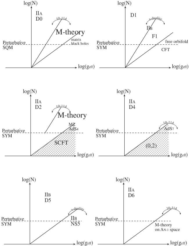
Figure 3: “Duality” between SYM with 16 supersymmetries and the supergravity of $D_{p}$ in the near horizon limit..

3.2 The quark anti-quark energy

By applying the procedure used in the previous section for ${\cal N}=4$ to the non-conformal, maximal supersymmetric backgrounds one finds for the energy of the quark anti-quark system (for $p\neq 5$)

$$E_{sg}\sim-({g_{YM}^{2}N\over L^{2}})^{1/(5-p)},$$ (17)

This result is valid as long as the range of $U$ we integrate over is in the allowed supergravity region. This implies that (i) The minimal value of $U$, $U_{0}$, has to be greater than the lower bound stated in (16), (ii) For $p<3$ since one cannot integrate up to $U=\infty$, to ensure a reasonable approximation one has to demand that $x(U_{ub})-L/2\ll L$, where $U_{ub}$ is the upper bound of $U$.

Generically for $p<3$ the result can be trusted only for the range 16 In certain cases we showed that in fact the range can be extended.

4 Wilson loops at finite temperature

We want to study the finite temperature effects on the Wilson line deduced from the supergravity solution [13, 15] We consider first that system that corresponds to the ${\cal N}=4$ SYM in four dimensions. For the finite temperature case the relevant solution is the near extremal solution which is Euclidean and periodic along the time direction. The period is the inverse of the Hawking temperature. The metric of the near extremal solution reads

$$ds^{2}=\alpha^{\prime}\left\{\frac{U^{2}}{R^{2}}[-f(U)dt^{2}+dx_{i}^{2}]+R^{2}f(U)^{-1}\frac{dU^{2}}{U^{2}}+R^{2}d\Omega_{5}^{2}\right\},$$

$$f(U)=1-U^{4}_{T}/U^{4},$$ (18)

$$R^{2}=\sqrt{4\pi gN},~{}~{}~{}~{}~{}~{}~{}~{}~{}~{}~{}U_{T}^{4}=\frac{2^{7}}{3}\pi^{4}g^{2}\mu~{},$$

where $\mu$ is the energy density above extremality on the brane and the Hawking temperature is $T=U_{T}/(\pi R^{2})$. The action is now

$$S = \frac{T}{2\pi}\int dx\sqrt{(\partial_{x}U)^{2}+(U^{4}-U_{T}^{4})/R^{4}}~{}~{}.$$ (19)

The “Hamiltonian” in the $x$ direction is now

$$\frac{U^{4}-U_{T}^{4}}{\sqrt{(\partial_{x}U)^{2}+(U^{4}-U_{T}^{4})/R^{4}}}=\mbox{const.}=R^{2}\sqrt{U_{0}^{4}-U_{T}^{4}},$$ (20)

so that $x$ as a function of $U$ is

$$x=\frac{R^{2}}{U_{0}^{3}}\sqrt{U_{0}^{4}-U_{T}^{4}}\int_{1}^{U/U_{0}}\frac{dy}{\sqrt{(y^{4}-1)(y^{4}-U_{T}^{4}/U_{0}^{4})}}~{}.$$ (21)

and in particular

$$L=2\frac{R^{2}}{U_{0}}\sqrt{\varepsilon}\int_{1}^{\infty}\frac{dy}{\sqrt{(y^{4}-1)(y^{4}-1+\varepsilon)}}$$ (22)

where $\varepsilon=1-U_{T}^{4}/U_{0}^{4}$.

What about the subtraction? We subtract the (infinite) mass of the W-boson which corresponds to a string stretched between the brane at $U=\infty$ and the $N$ branes at the horizon, $U=U_{T}$, and not at $U=0$. The reasons for this subtraction are: (i) It was shown that in the case of finite temperature the coordinates of the supergravity solution are not identical to the coordinates of the field theory living on the D-brane. A coordinate transformation is needed to match them. This transformation is such that from the point of view of the field theory living on the brane (at the one-loop order) the horizon is the origin. (ii) The Euclidean solution contains only the region outside the horizon. (iii) The local temperature close to the horizon is so high that it “burns” any static particle/string. The Our last argument is due to Hawking radiation. As is well known, due to the red shift-effect, the . In fact it is so high that any static will burn. In our case, by comparing the local temperature, $T_{loc}\sim T_{Haw}\sqrt{g^{tt}}$ to the string mass, $M_{s}=1/\sqrt{\alpha^{\prime}}$ The minimal distance for the string not to burn is $U_{T}(1+1/R^{2})\rightarrow U_{T}$ for $R\rightarrow\infty$.

Integrating from the horizon we obtain a finite result for the static energy

$$E=\frac{1}{\pi}\left\{U_{0}\int_{1}^{\infty}\left(\frac{\sqrt{y^{4}-1+\varepsilon}}{\sqrt{y^{4}-1}}-1\right)-U_{0}+U_{T}\right\}.$$ (23)

Figure 4: The distance $L$ between the quark-anti-quark pair as a function of $\epsilon=\epsilon(T,\tilde{U})$. Note that $L$ has a maximal value $L_{max}$.	Figure 5: The energy of the quark-anti-quark pair relative to the “free” quark situation as a function of $\epsilon=\epsilon(T,\tilde{U})$. Note that $E=0$ is achieved at $\epsilon_{C}<\epsilon_{max}$ corresponding to $L_{C}<L_{max}$.

We can extract from it $E(L,T)$ only numerically. At low temperature $TL\ll 1$

$$E=-{2\sqrt{2}\pi^{3/2}(4\pi g^{2}_{YM}N)^{1/2}\over\Gamma(1/4)^{4}}{1\over L}[1+c(TL)^{4}]$$ (24)

where $c$ is a positive numerical constant which does not depend on $R$. The underlying conformal nature of the theory reveals itself in the fact that $EL$ can depend on $T$ only through the combination $TL$. The behavior of $L$ as a function of $\epsilon$ seems a priori puzzling since following fig. 4 and fig. 5 $E(L,T)$ is double valued for $L>L_{max}$.

Fortunately physics tells us to believe the result only in the region $0<L<L_{C}$ where $L_{C}<L_{max}$. The existence of $L_{C}$ is seen in fig. 4. Starting from the low temperature region $\epsilon\sim 1$ we reach $\epsilon_{C}$ at which $E=0$. At this point the energy associated with our string configuration (fig. 5) is the same as the energy of a pair of free quark and anti-quark pair.

Note that $\epsilon_{C}$ is reached before $L$ reaches its maximal value $L_{max}$ (fig. 4).

Once we reach $L_{C}$ our string configuration (fig. 5) does not correspond to the lowest energy configuration which is $E=0$. For a given temperature $T$ we encounter two regions with different behavior. For $L<<1/T$ we observe a Coulomb like behavior while for $L>>1/T$ the quarks become free due to screening by the thermal bath. In fig 8. we have plotted $E=E(L)$ for a given $T$ by eliminating $\epsilon$ between eqs. (22) and (23) and trusting the result up to $L_{C}$.

Identical results are found for the correlation function of two temporal Wilson lines $W_{t}$ separated by a distance $L$

$$<W_{t}(0)W_{t}(L)>$$

Figure 6: The energetically favorable configuration for $L<L_{C}$.	Figure 7: The energetically favorable configuration for $L>L_{C}$.

Figure 8: The energy $E$ of the quark-anti-quark pair as a function of $L$ for a given $T$. The solid line corresponds to the numerical calculation up to $L_{C}$, the dashed line indicates the expected behavior for large $L$.

5 Area law behavior of Wilson lines from supergravity

Following the stringy interpretation of the Wilson loops of supersymmetric gauge theories at zero and finite temperature, a natural question to ask is whether one can detect, using the string/gauge duality, the confining nature of pure YM theory. We discuss here the computation in a setup that corresponds to “pure YM” theory in three dimensions, in four dimensional and finally we compute the ’t Hooft loop.

5.1 Confinement in 3 dimensional YM theory

The breaking of supersymmetry can be accomplished by choosing anti-periodic boundary conditions on the compactified time direction such that the ${\cal N}=4$ fermions and scalars acquire masses

$$m_{fermions}\sim T\qquad m_{scalars}\sim g_{YM4}^{2}T$$

Decoupling of these fields occurs in the limit of $T\rightarrow\infty$ of the Euclidean 4d temperature. The effective theory in this limit is known to be a gauge theory in 3d with a coupling

$$g_{YM_{3}}^{2}=g_{YM_{4}}^{2}T~{}.$$

The idea is, thus, to consider the Wilson loop along two space directions for the case of the near extremal D3 brane solution.

The metric of near extremal D3 branes in the large N limit is

$$ds^{2}=\alpha^{\prime}\left\{\frac{U^{2}}{R^{2}}[-f(U)dt^{2}+dx_{i}^{2}]+R^{2}f(U)^{-1}\frac{dU^{2}}{U^{2}}+R^{2}d\Omega_{5}^{2}\right\}$$

$$f(U)=1-U^{4}_{T}/U^{4}$$ (25)

$$R^{2}=\sqrt{4\pi gN},~{}~{}~{}~{}~{}~{}~{}~{}~{}~{}~{}U_{T}^{4}=\frac{2^{7}}{3}\pi^{4}g^{2}\mu~{},$$

where $\mu$ is the energy density. and we take one direction, $Y\rightarrow\infty$ and the other direction, $L$, to be finite. In this limit the wilson line is invariant under translation in the $Y$ direction. Therefore, for $LT\gg 1$, we obtain zero temperature non-supersymmetric Yang-Mills theory in three dimensions.

Using the (5.1) the relevant NG action for the spatial Wilson loop is

$$S=\frac{Y}{2\pi}\int dx\sqrt{\frac{U^{4}}{R^{4}}+\frac{(\partial_{x}U)^{2}}{1-U_{T}^{4}/U^{4}}}.$$ (26)

The distance between the quark and the anti-quark is

$$L=2\frac{R^{2}}{U_{0}}\int_{1}^{\infty}\frac{dy}{\sqrt{(y^{4}-1)(y^{4}-\lambda)}},$$ (27)

where $\lambda=U_{T}^{4}/U_{0}^{4}<1$ and $U_{0}$ is the minimal value of $U$. The energy is

$$E=\frac{U_{0}}{\pi}\int_{1}^{\infty}dy\left(\frac{y^{4}}{\sqrt{(y^{4}-1)(y^{4}-\lambda)}}-1\right)+\frac{U_{T}-U_{0}}{\pi},$$ (28)

Notice that in the limit $U_{0}\rightarrow U_{T}$ ($\lambda\rightarrow 1$) we get $L\rightarrow\infty$. In this limit the main contribution to the integrals in (27) and (28) comes from the region near $y=1$. Therefore, we get for large $L$

$$E=T_{QCD}L.$$ (29)

The tension of the QCD string is

$$T_{QCD}=\frac{\pi}{2}R^{2}T^{2},$$ (30)

Since both $T\rightarrow\infty$ and $R^{2}\rightarrow\infty$, it is clear that in these limit one cannot get a finite string tension. The hope is that the structure survives also when one penetrate to the small $R$ domain where obviously the supergravity approximation is not valid and one has to incorporate the full string theory.

Note also that the area law behavior, does not imply confinement in the 3+1 dimensional theory with temperature. This result interpolates between confinement in 2+1 dimensions ($LT\gg 1$) and Coulomb behavior in ${\cal N}=4$ YM in 3+1 dimensions ($LT\ll 1$). Is it really a 3d pure YM theory? The answer is that it is Not. There are varius reasons for that[16]. One obvious one is that it is a construction of ${\cal N}=4$ in 4d at $T\rightarrow\infty$ which is in fact not identical to pure YM theory in 3d. This manifest itself in the form of the meson meson interaction [10, 30] that is not dominated by a glueball exchange. A more general argument s that one cannot anticipate to deduce from gravity higher spin states like those one find along a Regge-trajectory. Nevertheless, it seems that the deviations do not change the basic fact tat it admits confinement.

5.2 Area law in four dimensional YM theory

The approach of the previous section to confinement can be generalized to obtain confinement in four dimensions from supergravity. We need to consider the supergravity solution of near-extremal D4-brane in the decoupling limit. A D4-brane is described in M-theory as a wrapped M5-brane so from the point of view of M-theory we relate the near-extremal solution of M5-brane to confinement in four dimensions as was suggested in sec. 4 of [26].

The near-extremal solution of D4-branes in the decoupling limit is [43]

$$ds^{2}=\alpha^{\prime}\left[\frac{U^{3/2}}{R_{4}^{3/2}}\left((1-U_{T}^{3}/U^{3})dx_{0}^{2}+dx_{1}^{2}+...+dx_{4}^{2}\right)+\right.$$

$$\left.\frac{R_{4}^{3/2}}{U^{3/2}(1-U_{T}^{3}/U^{3})}dU^{2}+R_{4}^{3/2}\sqrt{U}d\Omega^{2}_{4}\right],$$ (31)

$$e^{\phi}=\frac{1}{(2\pi)^{2}}g_{5}^{2}\left(\frac{U^{3}}{R^{3}}\right)^{1/4},$$

where $R_{4}^{3/2}=g_{5}\sqrt{\frac{N}{4\pi}}$ and $g_{5}$ is the 5D SYM coupling constant.

We would like to study the spatial Wilson loop in the region where $LT\gg 1$. In this region the effective description is via a non-supersymmetric YM theory in four dimensions with coupling constant

$$g_{YM}^{2}=g_{5}^{2}T.$$ (32)

Unlike the supergravity solution which was used in the previous section the supergravity solution (5.2), which we use here, cannot be trusted for arbitrary $U$. $L$, is related to $U$ by $L\sim 1/U$ and hence it is also bounded.

Before we perform the calculation of the spatial Wilson line let us first find the upper bound on $LT$ and the bounds on $g_{YM}$ and $g_{eff}^{2}=g_{YM}^{2}N$. The restrictions on $U$ and hence on $U_{T}$, are such that the curvature in string units and the effective string coupling are small. The result of these restrictions is (16) [43]

$$\frac{1}{Ng_{5}^{2}}\ll U_{T}\ll\frac{N^{1/3}}{g_{5}^{2}}.$$ (33)

Therefore, the supergravity solution can be trusted only for distances

$$Ng_{5}^{2}\gg L\gg\frac{g_{5}^{2}}{N^{1/3}}.$$ (34)

To find the bound on $T$ we use the relation between $T$ and $U_{T}$ (the temperature can be obtained from (5.2) and $\left.T=\frac{1}{4\pi}\frac{dg_{tt}}{dU}\right|_{U=U_{T}}$)

$$T=\frac{3\sqrt{\pi}}{g_{5}\sqrt{N}}\sqrt{U_{T}},$$ (35)

to get

$$\frac{1}{Ng_{5}^{2}}\ll T\ll\frac{1}{N^{1/3}g_{5}^{2}}~{}.$$ (36)

From (32) we find that the four dimensional coupling constant is bounded by

$$\frac{1}{N}\ll g_{YM}^{2}\ll\frac{1}{N^{1/3}}~{}.$$ (37)

We see, therefore, that in the large $N$ limit $g_{YM}$ must go to zero. For the four dimensional effective coupling, $g_{eff}$, we have

$$1\ll g_{eff}^{2}\ll N^{2/3}.$$ (38)

Thus the effective four dimensional coupling constant $g_{eff}$ must be large otherwise we cannot trust the supergravity description. Finally we turn to the bound for $TL$. To be able to use the supergravity results described below we need to find a region where $TL\gg 1$. From (34) and (55) we get

$$N^{2/3}\gg TL\gg\frac{1}{N^{4/3}}.$$ (39)

Therefore, in the large $N$ limit there is a region for which we can trust our results. Note that unlike the 3d case, considered in the previous section, in the 4d case, for any finite $N$, $L$ is bounded.

Let us now derive the area law behavior. The action for the string in this case is

$$S=\frac{Y}{2\pi}\int dx\sqrt{\frac{U^{3}}{R_{4}^{3}}+\frac{\partial_{x}U^{2}}{1-U_{T}^{3}/U^{3}}},$$ (40)

Using the same manipulations as in [8] we get

$$L=2\frac{R_{4}^{3/2}}{U_{0}^{1/2}}\int_{1}^{\infty}\frac{dy}{\sqrt{(y^{3}-1)(y^{3}-\lambda_{4})}},$$

$$E=\frac{U_{0}}{\pi}\int_{1}^{\infty}dy\left(\frac{y^{3}}{\sqrt{(y^{3}-1)(y^{3}-\lambda_{4})}}-1\right)+\frac{U_{T}-U_{0}}{\pi},$$ (41)

where $\lambda_{4}=\frac{U_{T}^{3}}{U_{0}^{3}}$. For $TL\gg 1$ we have $(U_{T}-U_{0})/U_{0}\ll 1$ and the integrals are dominated by the region close to $y=1$. Therefore, as in the previous section, we get

$$E=T_{YM}L$$ (42)

where the string tension is

$$T_{YM}=\frac{8}{27\pi^{2}}g_{YM}^{2}NT^{2}~{}.$$ (43)

This agrees with known large $N$ results if $T$ is identified with $\Lambda_{QCD}$ up to a $N$ independent constant factor.

5.3 ’t Hooft line

In YM theories the “ electric-magnetic” dual of the Wilson line is the ’t Hooft line. Just as one extract the quark anti-quark potential from the former, the later determines the monopole anti-monopole potential. We would like to address now the question of how to construct a supergravity model which associates with the ’t Hooft line.

Consider the supergravity background of near extremal $D_{4}$ branes 5.2. At large distances the effective theory is four dimensional along $x_{1},x_{2},x_{3},x_{4}$. The stringy realization of a monopole? is a D2-brane ending on the D4-brane. The D2-brane is wrapped along $x_{0}$ so from the point of view of the four dimensional theory it is a point like object. The BI action of a D2-brane is

$$S=\frac{1}{(2\pi\alpha^{\prime})^{3/2}}\int d\tau d\sigma_{1}d\sigma_{2}e^{-\phi}\sqrt{\mbox{det}h},$$ (44)

where $h$ is the induced metric. For the D2-brane we consider, which is infinite along one direction and winds the $x_{0}$ direction, we get

$$S=\frac{Y}{g_{YM}^{2}}\int dx\sqrt{\partial_{x}U^{2}+\frac{U^{3}-U_{T}^{3}}{R_{4}^{3}}},$$

where we have used (32). Note the $1/g_{YM}^{2}$ factor which is expected for a monopole. The distance between the monopole and the anti-monopole is

$$L=2\frac{R_{4}^{3/2}}{U_{0}^{1/2}}\sqrt{\epsilon}\int_{1}^{\infty}\frac{dy}{\sqrt{(y^{3}-1)(y^{3}-1+\epsilon)}}~{}.$$ (45)

where $\epsilon=1-(U_{T}/U_{0})^{3}$. The energy (after subtracting the energy corresponding to a free monopole and anti-monopole) is

$$E=\frac{2U_{0}}{(2\pi)^{3/2}g_{YM}^{2}}\left[\int_{1}^{\infty}dy\left(\frac{\sqrt{y^{3}-1+\epsilon}}{{\sqrt{y^{3}-1}}}\right)-1\right]+\frac{2(U_{T}-U_{0})}{(2\pi)^{3/2}}.$$ (46)

For $LT\gg 1$ it is energetically favorable for the system to be in a configuration of two parallel D2-branes ending on the horizon and wrapping $x_{0}$ So in the ”YM region” we find screening of the magnetic charge which is another indication to confinement of the electric charge.

6 Classical Wilson loops - general results

Equipped with the experience with the determination of the various loops in sections 1-5, we would like now to analyze the general setting We introduce here a space-time metric that unifies all these models and determine the corresponding static potential[19].

Consider a 10d space-time metric

$$ds^{2}=-G_{00}(s)dt^{2}+G_{x_{||}x_{||}}(s)dx^{2}_{||}+G_{ss}(s)ds^{2}+G_{x_{T}x_{T}}(s)dx^{2}_{T}$$ (47)

where $x_{||}$ are $p$ space coordinates on a $D_{p}$ brane and $s$ and $x_{T}$ are the transverse coordinates. The corresponding Nambu-Goto action is

$$S_{NG}=\int d\sigma d\tau\sqrt{det[\partial_{\alpha}x^{\mu}\partial_{\beta}x^{\nu}G_{\mu\nu}]}\\$$

Upon using $\tau=t$ and $\sigma=x$, where $x$ is one of the $x_{||}$ coordinates, the action for a static configuration reduces to

$$S_{NG}=T\cdot\int dx\sqrt{f^{2}(s(x))+g^{2}(s(x))(\partial_{x}s)^{2}}\\$$

where

$$f^{2}(s(x))\equiv G_{00}(s(x))G_{x_{||}x_{||}}(s(x))\qquad g^{2}(s(x))\equiv G_{00}(s(x))G_{ss}(s(x))$$ (48)

and $T$ is the time interval. The equation of motion (geodesic line) is

$$\frac{ds}{dx}=\pm\frac{f(s)}{g(s)}\cdot\frac{\sqrt{f^{2}(s)-f^{2}(s_{0})}}{f(s_{0})}$$

For a static string configuration connecting “Quarks” separated by a distance $L$ we therefore have

$$L=\int dx=2\int_{s_{0}}^{s_{1}}\frac{g(s)}{f(s)}\frac{f(s_{0})}{\sqrt{f^{2}(s)-f^{2}(s_{0})}}ds$$

The NG action and the corresponding energy $E={S_{NG}\over T}$ are divergent. The action is renormalized by subtracting the quark masses[8]. For the $AdS_{5}\times S^{5}$ case it is equivalent to the procedure suggested by [11].

$$m_{q}=\int_{0}^{s_{1}}g(s)ds$$ (49)

So that the renormalized quark anti-quark potential is

$$E=f(s_{0})\cdot L+2\int_{s_{0}}^{s_{1}}\frac{g(s)}{f(s)}(\sqrt{f^{2}(s)-f^{2}(s_{0})}-f(s))ds-2\int_{0}^{s_{0}}g(s)ds$$ (50)

The behavior of the potential is determined by the following theorem[19].

Theorem 1

Let $S_{NG}$ be the NG action defined above, with functions $f(s),g(s)$ such that:

1. $f(s)$ is analytic for $0<s<\infty$. At $s=0$, ( we take here that the minimum of $f$ is at $s=0$ ) its expansion is:

   $$f(s)=f(0)+a_{k}s^{k}+O(s^{k+1})$$

   with $k>0\;,\;a_{k}>0$.

2. $g(s)$ is smooth for $0<s<\infty$. At $s=0$, its expansion is:

   $$g(s)=b_{j}s^{j}+O(s^{j+1})$$

   with $j>-1\;,\;b_{j}>0$.

3. $f(s),g(s)\geq 0$ for $0\leq s<\infty$.

4. $f^{\prime}(s)>0$ for $0<s<\infty$.

5. $\int^{\infty}g(s)/f^{2}(s)ds<\infty$.

Then for (large enough) $L$ there will be an even geodesic line asymptoting from both sides to $s=\infty$, and $x=\pm L/2$. The associated potential is

1. if $f(0)>0$, then

   1. if $k=2(j+1)$,

      $E=f(0)\cdot L-2\kappa+O((\log L)^{\beta}e^{-\alpha L})$

   2. if $k>2(j+1)$,

      $E=f(0)\cdot L-2\kappa-d\cdot L^{-\frac{k+2(j+1)}{k-2(j+1)}}+O(L^{\gamma})$.

   where $\gamma={-\frac{k+2(j+1)}{k-2(j+1)}-\frac{1}{k/2-j}}$ and $\beta$,$\kappa$, $\alpha$ and $d$ are positive constants determined by the string configuration.

   In particular, there is linear confinement

2. if $f(0)=0$, then if $k>j+1$,

   $E=-d^{\prime}\cdot L^{-\frac{j+1}{k-j-1}}+O(L^{\gamma^{\prime}})$

   where $\gamma^{\prime}={-\frac{j+1}{k-j-1}-\frac{2k-j-1}{(2k-j)(k-j-1)}}$ and $d^{\prime}$ is a coefficient determined by the classical configuration.

   In particular, there is no confinement

A detailed proof of this theorem is given in [19].

6.1 Corollary- Sufficient conditions for confinement

A corollary that follows straightforwardly from the theorem states sufficient conditions for confinement. In fact two sufficient conditions can be extracted. Confinement occurs if either of the two conditions is obeyed:

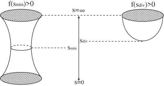
Figure 9: Sufficient conditions for confinement On the left a space-time with a metric such that $f$ has a minimum at $s_{min}$ with $f(s_{min})>0$ and on the right a space-time with horizon where $g$ diverges at $s_{div}$ and $f(s_{div})\neq 0.$

(i) $f$ has a minimum at $s_{min}$ and $f(s_{min})\neq 0$

or (ii) $g$ diverges at $s_{div}$ and $f(s_{div})\neq 0.$

In the case that there are several minima to $f$ it is the one with the greatest value of $s_{min}$ which is relevant. Models that obey the first condition $f(s_{min})\neq 0$ are characterized by having two disconnected boundaries (see fig. 9). The theory on the boundary can be made unitary only provided that the probability of propagating a physical signal from one boundary component to the other is negligible. Models that belong to the second condition have generically a boundary theory that relate to a bulk theory with an horizon.

6.2 Applications to various models

In the table below we summarize briefly the application of the theorem to the models discussed in sections 2-4 as well as some additional models of the rotating brane, the $D_{3}-D_{-1}$ system and MQCD.

Model	Nambu-Goto Lagrangian	Energy
$AdS_{5}\times S^{5}\cite[cite]{[\@@bibref{}{Mal2}{}{}]}$	$\sqrt{U^{4}/R^{4}+(U^{\prime})^{2}}$	$-\frac{2\sqrt{2}{\pi}^{3/2}R^{2}}{\Gamma(\frac{1}{4})^{4}}\cdot L^{-1}$
non-conformal
$D_{p}$ brane[43, 16]	$\sqrt{(U/R)^{7-p}+(U^{\prime})^{2}}$	$-d^{\prime}\cdot L^{-2/(5-p)}$
(16 susy)		$+O(l^{-2/(5-p)-2(6-p)/(5-p)(7-p)})$
Pure YM in 4d at		$\sim L^{-1}(1-c(LT)^{4})$ for $L<<L_{c}$
finite temperature	$\sqrt{(U/R)^{4}(1-(U_{T}/U)^{4})+(U^{\prime})^{2}}$	full screening $L>L_{c}$
[16, 15]
Dual model of
Pure YM in 3d	$\sqrt{(U/R)^{4}+(U^{\prime})^{2}(1-(U_{T}/U)^{4})^{-1}}$	$\frac{U_{T}^{2}}{2\pi R^{2}}\cdot L-2\kappa+O((\log L)^{\beta}\;e^{-\alpha L})$
[12, 16, 32, 31]
Dual model of
Pure YM in 4d	$\sqrt{(U/R)^{3}+(U^{\prime})^{2}(1-(U_{T}/U)^{3})^{-1}}$	$\frac{U_{T}^{3/2}}{2\pi R^{3/2}}\cdot L-2\kappa+O((\log L)^{\beta}\;e^{-\alpha L})$
Rotating $D_{3}$ [44]	$\sqrt{C}\sqrt{\frac{U^{6}}{U_{0}^{4}}\Delta+(U^{\prime})^{2}\frac{U^{2}\Delta}{1-a^{4}/U^{4}-U_{0}^{6}/U^{6}}}$	$4/3{U_{T}^{2}\over R^{2}}CL+...$
$D_{3}+D_{-1}$ [45]	$\sqrt{(U^{4}/R^{4}+q)+(U^{\prime})^{2}(1+qR^{4}/U^{4})}$	qL+…
$MQCD$ [18]	$2\sqrt{2\zeta}\sqrt{\cosh(s/R_{11})}\sqrt{1+s^{\prime 2}}$	$E=2\sqrt{2\zeta}\cdot L-2\kappa$
		$+O((\log L)^{\beta}\;e^{-1/\sqrt{2}R_{11}L})$
’t Hooft loop	$\frac{1}{g^{2}_{YM}}\sqrt{(U/R)^{3}(1-(U_{T}/U)^{3})+(U^{\prime})^{2}}$	full screening
[13, 17]		of monopole pair

7 Wilson loops associated with type 0 string models

Three avenues were taken recently on the way to extract information about non-superrsymmetric confining Wilson loops from classical supergravity effective actions. The first associated with the introduction of temperature was discussed in section 4. The second based on orbifolding of the $AdS_{5}\times S^{5}$[36] is not addressed in these lectures. The third option ( which is in fact equivalent to the second one) conjectures a duality between boundary gauge theories and type 0 string theories in the same spirit of the AdS/CFT correspondence. The determination of the potential in such scenario is the topic of this chapter which we start with a brief reminder of what are type 0 string theories.

7.1 What is a type 0 string theory

• Type 0 string is supersymmetric on the world sheet but not in space-time due to a non-chiral GSO projection. In 10d the massless spectra of type $0_{A}$ and $0_{B}$ string theory is given by

  $$type\ 0_{A}\ : (NS-,NS-)\oplus(NS+,NS+)\oplus(R+,R-)\oplus(R-,R+)$$

  $$type\ 0_{B}\ : (NS-,NS-)\oplus(NS+,NS+)\oplus(R+,R+)\oplus(R-,R-)$$ (51)

• The $(NS-,NS-)$ states (which are projected out in the type II theories) are the tachyons.

  The $(NS+,NS+)$ are the space-time metric $G_{\mu\nu}$ the NS $B_{\mu\nu}$ and the dilaton $\phi$.

  The states $(R+,R-)\oplus(R-,R+)$ for a doublet of the vector $A_{\mu}$ and $A_{\mu\nu\rho}$- the three form of the type $II_{A}$ and similarly $(R+,R+)\oplus(R-,R-)$ is a doubling of the axion $\chi$, the RR $B_{\mu\nu}$ and the self dual four form $C^{+}_{\mu\nu\rho\sigma}$.

• Thus, the type $0_{A}$ and type $0_{B}$ differ from the type $II_{A}$ and type $II_{B}$ in the following properties

  (i) No space-time fermions from the closed string sector.

  (ii) Doubling of the RR fields.

  (iii) Tachyons.

• The type 0 effective actions are consistent only provided (i) The Tachyon $m_{tach}^{2}$ can be shifted to $m_{tach}^{2}>0$ (ii) No dilaton ( and possible other massless fields) tadpoles (iii) Small string coupling and small curvature, $g_{st}<<1\qquad{\cal R}<<1$. It is plausible [21, 23] that due to the interaction with the RR fields the tachyons indeed loose their tachyonic nature. The absence of tadpoles was shown in string tree level. Generically , condition (iii) cannot be obtained throughout the whole range of scales but only in part of it.

• The low energy effective action of the type $0_{B}$ theories is composed of the $(NS+,NS+)$ sector which is identical to the one of type $II_{B}$, a tacyon sector, the RR sectors and the coupling of the later with the tachyon. The corresponding “ equations of motion” for $\phi,G_{\mu\nu},T$ and $C_{\mu\nu\rho\sigma}$ take the following form

  $$\phi : c_{0}+2\nabla^{\mu}\nabla_{\mu}\phi-4\nabla^{\mu}\phi\nabla_{\mu}\phi-{1\over 2}m^{2}T^{2}=0$$

  $$G_{\mu\nu} : R_{\mu\nu}+2\nabla_{\mu}\nabla_{\nu}\phi-\mbox{$\frac{1}{4}$}\nabla_{\mu}T\nabla_{\nu}T-{e^{2}\phi\over 96}f_{T}(T)(F_{\mu\cdot}F_{\nu}^{\ \cdot}-\mbox{$\frac{1}{10}$}G_{\mu\nu}F_{\cdot}F^{\cdot})=0$$

  $$T : (-\nabla^{\mu}\nabla_{\mu}+2\nabla^{\mu}\phi\nabla_{\mu}+m^{2})T-{e^{2}\phi\over 240}f^{\prime}_{T}(T)(F_{\cdot}F^{\cdot}=0$$

  $$C_{\mu\nu\rho\sigma} : \nabla_{\mu}[f_{T}(T)F^{\mu\nu\rho\sigma\tau}]=0$$ (52)

  where $c_{0}=-{D-10\over\alpha^{\prime}}$ describes a non-critical string, $f_{T}(T)=1+T+{1\over 2}T^{2}+...$ which may turn out to be $f_{T}(T)=e^{T}$. and $m^{2}={D-2\over 4\alpha^{\prime}}$.

• Since there is a doubling of the RR fields, one can have two types of theories. One in which only one type of RR field is turned on and the other when both. The former is referred to as the the electric theory or magnetic and the latter is the dyonic theory. In the dyonic case the flux of electric and magnetic RR field has to be equal. The interaction term between the tachyons and the RR fields is characterized by $h(T)=f(T),h(T)=f^{-1}(T)$ and $h(T)=f(T)+f^{-1}$ for the electric, magnetic and dyonic cases respectively.

7.2 The string/gauge correspondence and the Wilson loop

Before describing possible solutions of the equations, we discuss now the corresponding boundary gauge theories.

• The critical electric type $0_{B}$[21] theory with $N$ electric $D_{3}$ branes is conjectured to be dual to a non-supersymemtric $SU(N)$ gauge theory with six scalars in the adjoint.

• The dyonic theory on the other hand[23] does include fermions due to the open string between the electric and magnetic $D_{3}$ branes, thus constituting an $SU(N)\times SU(N)$ gauge theory with 6 adjoint scalars and 4 bifundamental fermions in the representation $(N,\bar{N})+(\bar{N},N)$.

• The five dimensional non-critical theories[25] correspond to a pure $SU(N)$ YM theory in the electric case and an $SU(N)\times SU(N)$ with fermions in one $(N,\bar{N})+(\bar{N},N)$ representation

• Solutions of the equations of motion were studied thoroughly for the critical case [21, 22]. Here we want to demonstrate the procedure of extracting the “ gauge theory properties” for the 5d non-critical case[25].

• We search for solutions of the equations 52 which are functions of the fifth coordinate only $\{\phi,G_{\mu\nu},T,F_{\cdot}\}(\rho)$. For the following parametrization of the metric

  $$dS^{2}=e^{-4\phi+4\lambda}d\rho^{2}+e^{2\lambda}dx_{\mu}^{2}$$

  the equations read

  $$\ddot{\Phi}+\mbox{$\frac{1}{2}$}(5+\mbox{$\frac{3}{16}$}T^{2})e^{-4\Phi+8\lambda}-\mbox{$\frac{5}{4}$}Q^{2}h(T)e^{-2\Phi+8\lambda}=0\ ,$$ (53)

  $$\ddot{\lambda}-\mbox{$\frac{3}{4}$}Q^{2}h(T)e^{-2\Phi+8\lambda}=0\ ,$$ (54)

  $$\ddot{T}+\mbox{$\frac{3}{4}$}Te^{-4\Phi+8\lambda}-2Q^{2}h^{\prime}(T)e^{-2\Phi+8\lambda}=0\ .$$ (55)

  

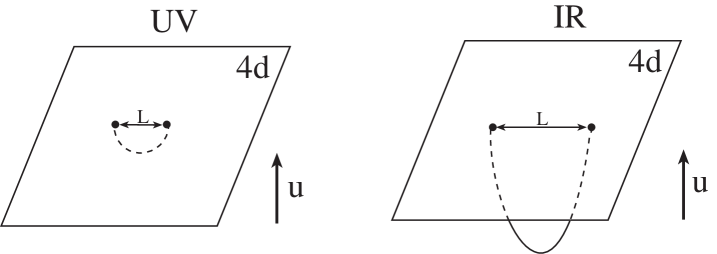
  Figure 10: The IR and UV regimes- For a small separation distance $L$ (left) the Wilson loop “explores” only the large $u$ region and for large $L$ (right) it reaches small values of $U$

• The dependence of the various fields on the fifth coordinate $\rho$ ( which was denoted in previous sections by $u$ or $s$) translates into the dependence of the gauge dynamics on the scale- the renormalization group flow. To test such a correspondence one has to identify what region of the fifth coordinate associates with the IR and UV regimes in the gauge picture. Clearly, due to the possibility to transform coordinates, the answer to this question should be based on a “meter” which is a physical quantity. Nothing is more natural in the present context than the use of the Wilson loop itself as the measuring device. From the two drawings above it is clear that the $u\rightarrow\infty$ region corresponds to small distance scales and hence to the UV regime and that the Wilson loop that stretch all the way to small values of $u$ ends on the boundary on points separated with a large distance, namely, it relates to the IR regime.

• From the equation of motion for the metric we find that $\ddot{\lambda}>0$[25] and hence the function $f$ defined in the theorem also has $\ddot{f}>0$. For boundary conditions such that $\dot{\lambda}<0$ the function $f$ has a minimum at some $\rho_{min}$ at which

  $$f(\rho_{min})>0$$

  Thus the solution obeys the first sufficient condition for confinement that was derived from the theorem of section 5. In fact one can show that this the structure of any generic solution, since the number of parameters (four) in solutions found by expanding around $\rho_{min}$ matches the dimension of the space of solutions.

• The conclusion is therefore that the generic solution to the equations of motion admits an area law behavior in the IR regime. Recall, however, that to have a unitary theory on the boundary at $u\rightarrow\infty$ one has to assure that no physical signal can propagate from this boundary to the other one at $\rho=0$.

• The confinement nature can also be verified using arguments based on the bulk 5d gauged-supergravity[42] and in particular from the screening nature of the ’t Hooft loop. It is also important to note that in this regime one can trust the supergravity solution since both the string coupling and the curvature are small. It is less clear to what extent a similar validity characterizes that UV regime.

• It was argued [21] that there is a UV fixed point which locally takes the form of an $AdS_{5}\times S^{5}$. Moreover around the fixed point $f$ behaves like a $logL$ so that it was argued [22] that

  $$\Delta V_{1}\sim{1\over log{L_{0}\over L}}{1\over L}$$

  namely, an asymptotic freedom behavior. Klebanov and Tseytlin [23] found that the higher order correction produces a WIlson line of the form

  $$\Delta V_{2}\sim{1\over log{L_{0}\over L}-clog\ log{L_{0}\over L}}{1\over L}$$

  which resembles the 2 loop correction in the gauge theory picture.

8 Quantum fluctuations

So far we have discussed Wilson loops from their correspondence to certain classical string configuration. Now we write down the machinery to incorporate quantum fluctuations and present some results about the QM determinant of some of the classical setups discussed above [34].

We start with introducing quantum fluctuations around the classical bosonic configuration

$$x^{\mu}(\sigma,\tau)=x^{\mu}_{cl}(\sigma,\tau)+\xi^{\mu}(\sigma,\tau)$$

The quantum correction of the Wilson line is

$$\langle W\rangle={\rm e}^{-E_{cl}(L)T}~{}\int\prod_{a}d\xi_{a}\exp\left(-\int d^{2}\sigma\sum_{a}\xi^{a}{\cal O}^{a}\xi^{a}\right)$$

where $\xi^{a}$ are the fluctuations left after gauge fixing. The corresponding free energy is

$$F_{B}=-\log{\cal{Z}}_{(2)}=-\sum_{a}{1\over 2}\log\det{\cal O}_{a}$$

8.1 Gauge fixing

In the classical treatment it is convenient to choose for the worldsheet coordinates $\tau=t$ and $\sigma=x$. In computing the quantum corrections it seems that there are several equivalent gauge fixings. One can still use the gauge of above, namely set $\xi_{x}=0$, or fix $\sigma=u,\ \xi_{u}=0$ (we denote here $s$ by $u$) so that there are no fluctuations in the space-time metric. However, it turns out that those gauges suffer from singularities at the minimum of the configuration $u_{0}$. A gauge that is free from those singularities is the “normal coordinate gauge” $\sigma=u_{cl}$ and the fluctuation in $x,u$ plane is in the coordinate normal to $u_{cl}$.

An important subtle issue is whether associated with these gauge fixings there are ghosts that have to be taken into account. As will be shown below it is clear that for the flat case there are none. The role of the ghosts for the non-trivial backgrounds is less clear.

8.2 General form of the bosonic determinant

In the $\sigma=u$ gauge and after a change of variables the free energy is given by

$$F_{B}=-{1\over 2}\log{\det{\cal O}_{x}}-{(p-1)\over 2}\log{\det{\cal O}_{x_{II}}}-{(8-p)\over 2}\log{\det{\cal O}_{x_{T}}}$$ (56)

where

$$\hat{\cal O}_{x} = \left[\partial_{x}\left((1-{f^{2}(u_{0})\over f^{2}(u_{cl})})\partial_{x}\right)+{G_{xx}(u_{cl})\over G_{tt}(u_{cl})}({f^{2}(u_{cl})\over f^{2}(u_{0})}-1)\partial_{t}^{2}\right]$$

$$\hat{\cal O}_{x_{II}} = \left[\partial_{x}\left({G_{y_{i}y_{i}}(u_{cl})\over G_{xx}(u_{cl})}\partial_{x}\right)+{G_{y_{i}y_{i}}(u_{cl})\over G_{tt}(u_{cl})}{f^{2}(u_{cl})\over f^{2}(u_{0})}\partial_{t}^{2}\right]$$

with $\hat{\cal O}={2\over f(u_{0})}{\cal O}$ and a similar expression for $\hat{\cal O}_{x_{T}}$. The boundary conditions are $\hat{\xi}(-L/2,t)=\hat{\xi}(L/2,t)=0$

8.3 Bosonic fluctuations in flat space-time

Let us recall first the determinant in flat space-time. The fluctuations in this case are determined by the following action

$$S_{(2)}={1\over 2}\int d\sigma d\tau\sum_{i=1}^{D-2}\left[\left(\partial_{\sigma}\xi_{i}\right)^{2}+\left(\partial_{\tau}\xi_{i}\right)^{2}\right]$$

The corresponding eigenvalues are

$$E_{n,m}=({{n\pi\over L}})^{2}+({{m\pi}\over T})^{2}$$

and the free energy is given by

$$-\frac{2}{D-2}F_{B}=\log\prod_{nm}E_{n,m}=T{\pi\over 2L}\sum_{n}n+O(L)$$

Regulating this result using Riemann $\zeta$ function we find that the quantum correction to the linear quark anti-quark potential is

$\Delta V(L)=-{1\over T}F_{B}=-(D-2){\pi\over 24}\cdot{1\over L}$

which is the so-called Lüscher term[1].

8.4 General scaling relation, and the $L$ dependence of $\Delta V$

Consider an operator of the form

$${\cal O}[A,B]=A^{2}F_{t}(v)\partial_{t}^{2}+B^{2}\partial_{v}({\cal O}_{v})$$

where $v$ is a coordinate whose range is independent of $L$ The correction to the potential $V[A,B]$ due to fluctuations determined by such an operator is

$$V[A,B]=(B/A)\cdot V[1,1]$$

For the operators that describe the fluctuations associated with metrics such that

$$f(u)=au^{k}\qquad g(u)=bu^{j}$$ (58)

like for instance for the $D_{p}$ brane solution in the near horizon limit we find that $A^{2}=bu_{0}^{j}\;,\;B^{2}=\frac{a^{2}}{b}u_{0}^{2k-j-2}\rightarrow B/A=\frac{a}{b}u_{0}^{k-j-1}$ Therefore, the potential is proportional to

$B/A=\frac{a}{b}u_{0}^{k-j-1}\rightarrow\Delta V\propto L^{-1}$

Thus, the quantum correction of the quark anti-quark potential is of Lüscher type[1]for models of $D_{p}$ branes with 16 supersymmetries, in particular also the $AdS_{5}\times S^{5}$ model.

8.5 The fermionic fluctuations in flat space-time

The NSR action of the type II superstring with RR fields like on $AdS_{5}\times S^{5}$ is not known. On the other hand the manifestly space-time supersymmetric Green Schwarz action was written down for the $AdS_{5}\times S^{5}$ case[47] To demonstrate the use of the GS action we start with the fermionic determinant in flat space-time

The fermionic part of the $\kappa$ gauged fixed GS-action is

$$S_{F}^{flat}=2i\int d\sigma d\tau\bar{\psi}\Gamma^{i}\partial_{i}\psi$$

where $\psi$ is a Weyl-Majorana spinor, $\Gamma^{i}$ are the SO(1,9) gamma matrices, $i,j=1,2$ and we explicitly considered a flat classical string. Thus the fermionic operator is

$$\hat{\cal O}_{F}=D_{F}=\Gamma^{i}\partial_{i}\qquad(\hat{\cal O}_{F})^{2}=\Delta=\partial_{x}^{2}-\partial_{t}^{2}$$

The total free energy is

$$F=8\times\left(-{1\over 2}\log\det\Delta+\log\det D_{F}\right)=0$$

since for D=10, we have 8 transverse coordinates and 8 components of the unfixed Weyl-Majorana spinor. Thus in flat space-time the energy associated with the supersymmetric string is not corrected by quantum fluctuations.

8.6 The determinant for a free BPS quark of $AdS_{5}\times S^{5}$

The $\kappa$ fixed GS action[47] is based on treating the target space as the coset $SU(2,2|4)/(SO(1,4)\times SO(5))$. The action incorporates the coupling to the RR field. The square of the operator associated with the fermionic fluctuations of a BPS string representing a single quark is

$$8\times\ \left({\cal O}^{2}_{\psi}=({R\over u})^{2}\partial_{t}^{2}+({u\over R})^{2}\partial_{u}^{2}-{7/4\over R^{2}}\right)$$

where $R$ is the $AdS_{5}\times S^{5}$radius. The bosonic operators are of the form

$$3\times[{\cal O}_{x} = ({R\over u})^{2}\partial_{t}^{2}+({u\over R})^{2}\partial_{u}^{2}-{3\over R^{2}}$$

$$5\times[{\cal O}_{\theta} = ({R\over u})^{2}\partial_{t}^{2}+({u\over R})^{2}\partial_{u}^{2}-{7/4\over R^{2}}]$$

where $\{t,x,u,\theta\}\equiv\{\tau,{\xi\over u},\sigma,\xi_{\theta}\}$ and $\theta$ is the coordinate on the $S^{5}$ According to a theorem of McKean and Singer[49] the divergences of a Laplacian type operator of the form

$$\Delta=\nabla^{2}+X=-{1\over\sqrt{g}}D_{a}(g^{ab}\sqrt{g}D_{b})+X$$

vanishes if there is a match between the fermionic and bosonic coefficients of $\nabla^{2}$ and $X$. In the present case there are $8$ bosonic and $8$ fermionic $\nabla^{2}$ terms and hence there is no quadratic divergences, and the coefficients of $X$ are $8\times 7/4$ from the fermions and $3\times 3+5\times 1$ from the bosons so there are also no logarithmic divergences. It is thus clear that the divergent parts of the determinant associated with the supersymmetric fluctuation of a BPS string “quark” vanish. This problem is related to issues associated with certain BPS soliton solutions[50].

8.7 The determinant for a Wilson line of $AdS_{5}\times S^{5}$

The GS action was further simplified by using a particular $\kappa$ fixing[48]

$$S_{GS} = \int d^{2}\sigma[\sqrt{g}g^{\alpha\beta}(y^{2}[\partial_{\alpha}x^{p}-2i\bar{\psi}\Gamma^{p}\partial_{\alpha}\psi][\partial_{\beta}x^{p}-2i\bar{\psi}\Gamma^{p}\partial_{\beta}\psi]$$

$$+ {1\over y^{2}}\partial_{\alpha}y^{t}\partial_{\beta}y^{t})+4\epsilon^{\alpha\beta}\partial_{\alpha}y^{t}\bar{\psi}\Gamma^{t}\partial_{\beta}\psi]$$

where $\psi$ is a Majorana-Weyl spinor and the $Ads_{5}\times S^{5}$ metric is written in terms of the $4+6$ coordinates $ds^{2}=y^{2}dx_{II}^{p}dx_{II}^{p}+{1\over y^{2}}dy^{i}_{x_{T}}idy^{i}_{x_{T}}$ The bosonic operators in the normal gauge now read

$$2\times\qquad{\cal O}_{x_{II}}\ \ \ = \partial_{x}^{2}-{u^{4}\over u_{0}^{4}}\partial_{t}^{2}$$

$$5\times\qquad{\cal O}_{\theta}\ \ \ = \partial_{x}^{2}-{u^{4}\over u_{0}^{4}}\partial_{t}^{2}+2{u^{6}\over u_{0}^{4}}$$

$$1\times\qquad{\cal O}_{normal} = \partial_{x}^{2}-{u^{4}\over u_{0}^{4}}\partial_{t}^{2}+5u^{2}-3{u^{4}\over u_{0}^{2}}$$

The fermionic part of the action for the classical solution leads to the operator

$$\hat{\cal O}^{2}_{\psi}={u_{0}^{2}\over R^{2}}\Gamma^{1}\partial_{x}+\left({u_{cl}^{4}\over{u_{0}^{2}R^{2}}}\Gamma^{0}+{u_{cl}^{4}\over R^{4}}\cdot{\sqrt{u_{cl}^{4}-u_{0}^{4}}\over u_{0}^{2}}\Gamma^{2}\right)\partial_{t}$$

where we use $\Gamma$ matrices of SO(1,4), the $AdS_{5}$ tangent space. Squaring this operator, we find

$$\left({R^{2}\over u_{0}^{2}}\hat{\cal O}_{F}\right)^{2}=\partial_{x}^{2}-{u_{cl}^{4}\over u_{0}^{4}}\partial_{t}^{2}={R^{2}\over u_{0}^{2}}\hat{\cal O}_{II}$$

Thus the transverse fluctuations ${\cal O}_{x_{II}}$ are cancelled by the fermionic fluctuations. We are left with 6 fermionic degrees of freedom, the normal bosonic fluctuation and 5 additional bosonic fluctuations associated with ${\cal O}_{\theta}$. Using our general result we know that the quantum correction of the potential is of a Luscher type. The universal coefficient and in particular its sign has not yet been determined.

In [51] the bosonic and fermionic determinants were analyzed in a different gauge fixing procedure. The 2d reparametrization invariance was treated in the Riemann normal coordinates and a diffent fixing of the $\kappa$ symmetry was invoked. Using these gauge fixings a closed expression for the supersymmetric determinant was written down.

$$W(C)=e^{-A_{R}}\;{\det\left(-\Delta_{F}-{1\over 4}R^{(2)}+1\right)\over\det\left(-\Delta_{cl}+2\right)\det^{{1\over 2}}\left(-\Delta_{cl}+4-R^{(2)}\right)\det^{{5\over 2}}\left(-\Delta_{cl}\right)}$$ (62)

where $A_{R}$ is the regulated area, $\Delta_{cl}$ is the classical Laplacian and $\Delta_{F}=g^{\alpha\beta}\nabla_{\alpha}\nabla_{\beta}$ The corresponding free energy suffers from logarithmic divergences. It was suggested to renormalize the quark masses to get read of this divergence.

8.8 The determinant for “confining scenarios”

Let us consider first the the setup which is dual to the pure YM theory in 3d. For that case where the Euclidean coordinate is compactified

$$f(u)=u^{2}/R^{2}\qquad g(u)=(1-(\frac{u_{T}}{u})^{4})^{-1/2}$$ (63)

so that $g$ diverges at the horizon $u=u_{T}$. In the large $L$ limit

$$\hat{\cal O}_{x_{II}} \longrightarrow \frac{u_{T}^{2}}{2R^{2}}\left[\partial_{x}^{2}+\partial_{t}^{2}\right]$$

$$\hat{\cal O}_{t} \longrightarrow {u_{T}^{2}\over 2R^{2}}e^{-2u_{T}L}\left[\partial_{x}^{2}+\partial_{t}^{2}\right]$$

$$\hat{\cal O}_{\theta} \longrightarrow \left[\frac{R^{2}}{2}[\partial_{x}^{2}+\partial_{t}^{2}\right]$$ (64)

We see that the operators for transverse fluctuations, $\hat{\cal O}_{x_{II}}$, $\hat{\cal O}_{t}$, turn out to be simply the Laplacian in flat spacetime, multiplied by overall factors, which are irrelevant. Therefore, the transverse fluctuations yield the standard Lüscher term proportional to $1/L$. The longitudinal normal fluctuations give rise to an operator $\hat{\cal O}_{n}$ corresponding to a scalar field with mass $2u_{T}/R^{2}=\alpha$. Such a field contributes a Yukawa like term

$$\approx-\frac{\sqrt{\alpha}e^{-\alpha L}}{\sqrt{L}}$$

to the potential. Thus, in the metric that corresponds to the “pure YM case” there are 7 Luscher type modes and one massive mode. It can be shown that a similar behavior occurs in the general confining setup [34]. Had the fermionic modes been those of flat space-time then the total coefficient in front of the Luscher term would have been a repulsive Culomb like potential[31] which contradicts gauge dynamics[52]. However the point is that due to the RR flux the corresponding GS action cannot be that of a flat space-time. Indeed the fermionic fluctuations also become massive so that the total interaction is attractive after all which is in accordance with [32].

9 On the exact determination of stringy Wilson loops

So far we have discussed the determination of Wilson loops from the classical string and the way quantum fluctuations modify the classical result. An interesting question to address is whether in certain circumstances one can find an exact expression for the Wilson loop. Such an exact result was derived for the simplest case of a string in flat space-time. Since the derivation was originally done in terms of the energy of the sting in the Polyakov formulation, we first show that for a static case the latter is equal to the NG action ( for a diagonal space-time metric).

Recall the form of the Polyakov action in the covariant world sheet gauge

$$S_{Poly}=T_{st}\int d^{2}\sigma\partial_{\alpha}X^{\mu}\partial^{\alpha}X^{\nu}G_{\mu\nu}(X)$$ (65)

and the corresponding space-time energy

$$E=T_{st}\int_{0}^{\pi}d\sigma\partial_{\tau}X^{\mu}G_{\mu 0}$$

Consider a classical configuration that associates with a “Wilson loop” along the two coordinates $X(\sigma)$ , $u(\sigma)$ and the rest of the coordinates are set to zero, with the following boundary conditions

$$X^{1}(0)=0;X^{1}(\pi)=L;\qquad u(0)=u(\pi)=\infty;\qquad X^{0}=\tau$$

Using the equations of motion it is a straightforward exercise to show that

$$S_{NG}\sim E=\int_{u_{0}}^{\infty}{du\over\partial_{x}u}{f^{2})\over f_{0}}$$ (66)

where $x=X^{1}$, $f$ and $f_{0}$ were defined in section 5.

Consider now the bosonic string in flat space-time which implies that it stretches only along $x$ with the boundary conditions of above.

$$X^{1}(\sigma\tau) = {L\over\pi}\sigma+\sum_{n=1}^{\infty}{\alpha^{i}_{n}\over n}sin(n\sigma)e^{-in\tau}$$

$$X^{0}(\sigma\tau) = 2\pi\alpha^{\prime}E\tau+i\sum_{n=1}^{\infty}{\alpha^{0}_{n}\over n}cos(n\sigma)e^{-in\tau}$$

The energy of the lowest tachyonic state is given by

$$E^{2}=P^{i}P_{i}+m_{tach}{{}^{2}}=({L^{i}\over 2\pi\alpha^{\prime}})^{2}-{(D-2)\over 24}{1\over\alpha^{\prime}}\\$$

so that[3]

$E=T_{st}L\sqrt{1-{(D-2)\over 24}{1\over T_{st}L^{2}}}$

For $L>>(T_{s})^{-1/2}$ this can be expanded to yield

$$\sim T_{st}L-\pi{(D-2)\over 24}{1\over L}+...$$

where the string tension $T^{-1}_{st}=2\pi\alpha^{\prime}$. Thus this expansion yields the Luscher quadratic fluctuation term.

Moreover, this result is identical to the expression for the NG action derived for a bosonic string in flat space-time in the large $D$ limit[2]

$$D\rightarrow\infty\qquad{\pi\over 24T_{st}L^{2}}\rightarrow 0\qquad{D\pi\over 24T_{st}L^{2}}\rightarrow finite$$

A more challenging question is whether one can find such “exact” solution for a non-flat space-time. A naive conjecture is that for the $Ads_{5}\times S^{5}$ the result is $\sim-{\sqrt{g^{2}N}\over L}\sqrt{1+{c\over\sqrt{g^{2}N}}}$. However, whereas its large $g^{2}N$ expansion includes the result of [8] and a non trivial Luscher term, it does not permit a smooth extrapolation to the weak coupling region where the potential behaves like $\sim-{g^{2}N\over L}$.

10 Wilson loops for string actions with a $B_{\mu\nu}$ background

Exact results are known for non trivial backgrounds of group manifolds and coset spaces. That is one motivation to re-examine Wilson loops in the presence of $B_{\mu\nu}$ background which is an essential part of the action of a string on group manifold. In fact there are other independent reason to study this case. One additional reason is the $AdS_{3}$ string theory that attracted recently a lot of attention and another one is the world-sheet approach to non-commutative geometry.

The bosonic action in the presence of a WZ term can be written as

$$S_{B}=S_{NG}+\int d^{2}\sigma e^{\alpha\beta}\partial_{\alpha}X^{\mu}\partial_{\beta}X^{\nu}B_{\mu\nu}$$

For the application of using the string action to compute the Wilson loop we consider a classical string configuration where $X^{0}(\tau)=\tau$ and the only non trivial coordinates are $X^{1}(\sigma)\equiv x(\sigma)$ and $u(\sigma)$. For such configurations the only components of $B_{\mu\nu}$ that can contribute are $B_{01}\equiv B$ and $B_{0u}\equiv B_{u}$. We consider here the case that only $B_{01}\equiv B$ is non-trivial. In the coordinate choice $\tau=x^{0}$ and $\sigma=x$ the WZ term takes the form $S_{WZs}=T\int dx[B(x)]$. Assuming again a diagonal metric, the action in the static gauge takes the form

$$S_{NG+WZ}=T\int dx[\sqrt{f^{2}+g^{2}(\partial_{x}u)^{2})}-B(x)]$$ (68)

were $f$ and $g$ were defined in section 5. The equation of motion for this action takes the form

$${f^{2}\over\sqrt{f^{2}+g^{2}(\partial_{x}u)^{2})}}-B=f_{0}-B_{0}$$ (69)

where $f_{0}$ and $B_{0}$ are the values of $f$ and $B$ respectively at $u_{0}$ where $u^{\prime}=0$. For the case that $f=B$ having $u^{\prime}=0$ at one point implies $u^{\prime}=0$ everywhere. Moreover, in this case the action of the classical configuration vanishes.

Consider the case where $f\neq B$. A particular simple case is when $B$ is a constant. Obviously for closed string the WZ term for such a case is a total derivative and hence vanishes, however for the open string it is not. The equations of motion are not modified and the action is just the NG action plus an additional term of the form $S_{B}=TLB$. Note that such a correction translates into an addition of a linear potential to the quark anti-quark interaction.

Using the boundary conditions the value of $u_{0}$ is related to $L$ as follows

$$L/2=\int_{u_{0}}^{\infty}{du}={g\over f}{f_{0}+B-B_{0}\over\sqrt{f^{2}-(f_{0}+B-B_{0})^{2}}}$$ (70)

The action for a configuration that solves the equation of motion is

$$S_{NG+WZ}=T\int_{u_{0}}^{\infty}{du}{g\over f}{f^{2}-B(f_{0}+B-B_{0})\over\sqrt{f^{2}-(f_{0}+B-B_{0})^{2}}}$$ (71)

We can now determine the relation between the quark anti-quark potential and the separation disctance $L$ as follows

$$E{q\bar{q}}=(f_{0}-B_{0})L+2\int_{u_{0}}^{\infty}du{g\over f}\sqrt{f^{2}-(f_{0}+B-B_{0})^{2}}$$ (72)

since $E_{q\bar{q}}={S_{NG}\over T}$

It is thus clear that for $f=B$ indeed the action and hence the energy vanish. For sting theoris where $f_{0}-B_{0}$ does not vanish the Wilson loop admits an area law behaviour with a string tension equal to $f_{0}-B_{0}$. This resutl holds provided that the second term is sub leading. For the pure NG case ( with no WZ tern) this was proven in the theorem (see section 5) and the next to leading classical correction was found to be of the order $O(logLe^{-\alpha L})$.

In the case with no $B$ the NG action was renormalized by substructing the “masses of the two quarks”, namely, $S_{Ren}=S-2\int_{0}^{\infty}dug(U)$ (For a space-time metric that admits an horizon at $u=u_{T}$ the range of integration starts from $u_{T}$ and not from $u=0$.) A natural question is how to renomalize the $S_{NG+WZ}$ action. It is obvious now that a straight line with $\partial_{x}u=\infty$ is not a solution of the equation of motion. So one has to substruct the action associated with the quark string $S_{Ren}=S-2S^{quark}$

Let us analyze now the Wilson loop of a string in an $Ads_{3}$ background and in particular the $SL(2R)$ WZW model. The action takes the form

$${\cal L}_{SL(2R)}=\sqrt{(\partial_{x}u)^{2}+u^{4}}-\alpha u^{2}$$ (73)

where the values of $\alpha$ are $\pm 1$ associated with the two possible orientation of the string connecting the points $x=0$ and $x=L$. The equation of motion now reads

$$\alpha u^{2}-{u^{4}\over\sqrt{(\partial_{x}u)^{2}+u^{4}}}=(\alpha-1)u_{0}^{2}$$

where $u_{0}$ is a minimum of $u$ where $(\partial_{x}u)=0$.

For $\alpha=1$ the solution is that $(\partial_{x}u)=0$ everywhere and thus the classical configuration that connects the two points on boundary is just a straight line on the boundary. This is a BPS string of zero energy. For $\alpha=-1$ again one cannot connect two points at finite separation distance by a string that penetrates the bulk. As for the full exact quantum energy. It is clear that in the superstring case there would not be any quantum corrections. However, for the bosonic string theory one anticipates to have a Luscher term as the full answer of the following form $E={{3\over 1-2/k}+21\over 24}{1\over L}$ where $k$ is the level of the WZW model.

It seems that always in a WZW theory with aboundary the value of the action at the extremum vanishes. In that case the only solution is that $u^{\prime}=0$ every where and so the two points on the boundary are necessarily connected by a straight line so the energy (which is zero ) is not a function of $L$. In a similar manner coset models based on a WZW theory with a boundary can be analyzed.

11 Baryon Configurations from string ( supergravity) models

Consider now on the AdS surface $N_{c}$ external quarks. What is the string system that can connect them? Clearly a string cannot connect a pair of quarks ( only a pair of a quark anti-quark). Alternatively the $N$ quarks can be connected to a Baryon vertex The question is how can we construct such a baryon vertex from the building blocks of the type $II_{B}$ on the backgroud? Witten [26] proposed a baryon vertex which is based on a a five brane wrapped on the $S^{5}$ located at a certain point of the $AdS_{5}$. The type $II_{B}$ self-dual five-form field $G_{5}$ has a flux of $N_{c}$ unites coming out the $S^{5}$. $\int_{S^{5}\times R}{G_{5}\over 2\pi}=N$ On the $D_{5}$ world volume there is a coupling of $G_{5}$ to an abelian gauge field

$$\int_{S^{5}\times R}a\wedge{G_{5}\over 2\pi}$$

So the $G_{5}$ contributes $N$ unites of $a$ charge. The total charge in the $S^{5}$ closed universe has to vanish. The strings behave as fermions so that the $N$ quarks are in a completely antisymmetric representation

$N$ strings ending on the $D_{5}$ brane provide this needed charge

11.1 Baryons of ${\cal N}=4$ SYM in four dimensions

The baryons of the ${\cal N}=4$ SYM theory are BPS states. The BPS equations associated with the worldvolume Born-Infeld plus WZW action of a D5-brane in the background of N D3-branes were studied in [28, 29]. BPS-exact solutions were constructed. A Hanany-Witten type mechanism was invoked in the case that a D5-brane is dragged across a stack of N D3-branes. It was shown that a bundle of N fundamental strings joining the two types of branes is created. tes via the AdS/CFT correspondence.

Since we have in mind that our aim is the study of baryons in confining non-supersymmetric models, where the notion of a BPS state does not apply we use here a different approach which is based on a “zero order” account of the action[27]. In such an approach we consider independet contributions to the action from the baryonic vertex and the strings, namely

$$S_{total}=S_{D5}+NS_{1F}.$$ (74)

(i)The first contribution comes from the string stretched between the boundary of the AdS₅ space and the D5-brane wrapped on the $S_{5}$.

(ii) The second contribution comes from the D5-branes itself. a static D5-brane wrapped on $S^{5}$

$$S_{D5}=\frac{1}{(2\pi)^{5}{\alpha^{{}^{\prime}}}^{3}e^{\phi}}\int dx^{6}\sqrt{h}=\frac{TNU_{0}}{8\pi},$$ (75)

where $U_{0}$ is the location of the baryon vertex in the bulk, $T$ is the time period which we take to infinity and $h$ is the induced metric on the fivebrane.

$$S_{1F}=\frac{T}{2\pi}\int dx\sqrt{U_{x}^{2}+U^{4}/R^{4}},$$ (76)

where $U_{x}=\frac{\partial U}{\partial x}$ and $R^{4}=4\pi g_{s}N$.

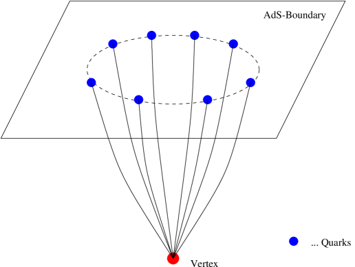
Figure 11: The Baryon Vertex

The configuration which we consider ( see Fig. 11) is such that the strings end on a surface with radius $L$ in a symmetric way.

The stability conditions for a consistent baryonic configuration are the following:

(i) The symmetric quark configuration ensures that

$$\sum F_{x_{i}}=0$$

(where $x_{i}$ are the direction along the boundary where the field theory is living.

(ii) Along the $U$ direction the no-force condition is

$$\delta U\frac{TN}{8\pi}=\delta U\frac{TN(U_{x})_{0}}{2\pi\sqrt{(U_{x})_{0}^{2}+U_{0}^{4}/R^{4}}},$$ (77)

where $(U_{x})_{0}=\frac{\partial U}{\partial x}|_{U_{0}}$ and $\delta U$ is the variation of $U$ at $x=0$ where the string hits the baryon vertex.

This condition can be derived as follows The variation of (74) under $U\rightarrow U+\delta U$ contains a volume term as well as a surface term. The volume term leads to the Euler-Lagrange equation whose solution satisfies [43]

$$\frac{U^{4}}{\sqrt{U_{x}^{2}+U^{4}/R^{4}}}=\mbox{const.}$$ (78)

because the action does not depend explicitly on $x$. The surface term yields the no force conditoin.

This implies the following relation between $U_{0}$ and the radius of the baryon $L$

$$L=\frac{R^{2}}{U_{0}}\int_{1}^{\infty}\frac{dy}{y^{2}\sqrt{(\beta^{2}y^{4}-1)}}~{}$$ (79)

where $\beta=\sqrt{16/15}$. The energy of a single string is given by

$$E=\frac{1}{2\pi}U_{0}\left(\int_{1}^{\infty}dy\frac{\beta y^{2}}{\sqrt{\beta^{2}y^{4}-1}}-1\right)-\frac{U_{0}}{2\pi}$$ (80)

Where we subtract the energy of the configuration with the D5-brane located at $U=0$. Since $g_{xx}$ vanishes at $U=0$ any radial string which reaches this point ends on the D5-brane. As a result the energy of the fermionic strings, which we subtract equals the energy of free quarks. Note that since $g_{tt}(U=0)=0$ the contribution of the D5-brane located at $U=0$ to the energy vanishes.

Inserting the relation (79) into (80) one finds that the energy of each string is

$$E=-\alpha_{st}{\sqrt{2g_{YM}^{2}N}\over L},~{}~{}\mbox{where}~{}~{}\alpha_{st}=~{}\frac{1}{4}\sqrt{\frac{5}{6\pi}}{}_{2}F_{1}[\frac{1}{2},\frac{3}{4},\frac{7}{4};\frac{15}{16}]\times{}_{2}F_{1}[\frac{1}{2},-\frac{1}{4},\frac{3}{4};\frac{15}{16}]\simeq 0.036$$ (81)

The total energy of the baryon configuration is therefore

$$E=-\alpha_{B}N{\sqrt{2g_{YM}^{2}N}\over L},~{}~{}\mbox{where}~{}~{}\alpha_{B}=...\simeq 0.007$$ (82)

Since the force $F=\frac{dE}{dL}$ is positive the baryon configuration is stable. Moreover, as expected from the field theory large N analysis, the energy is proportional to $N$ times that of the quark anti-quark system.

11.2 Baryons in non-SUSY theories

We discuss YM in three dimensions (the generalization to the four dimensional case is straight forward). The supergravity solution associated with pure YM in three dimensions is given by the near-extremal D3-branes solution in the decoupling limit

$$ds^{2}=\frac{U^{2}}{R^{2}}\left[-(1-\frac{U_{T}^{4}}{U^{4}})dt^{2}+\sum_{i=1}^{3}dx_{i}^{2}\right]+\frac{R^{2}}{U^{2}(1-\frac{U_{T}^{4}}{U^{4}})}dU^{2}+R^{2}d\Omega_{5}^{2}~{}.$$ (83)

To obtain three dimensional theory we need to go to the IR limit and to consider distances (along $x_{1},x_{2},x_{3}$) which are much larger then $1/T$. At the region where we can trust the supergravity solution, $R^{2}\geq 1$, the theory is not quite three dimensional YM theory. Nevertheless, it does possess the properties of YM in three dimensions which are relevant to the present discussion [12, 16, 46, 53].

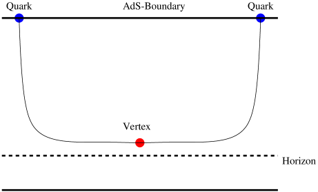
Figure 12: The baryon in non supersymmetric theories

The surface term gives

$$\frac{1}{4}=\frac{U_{0}^{\prime}}{(1-U_{T}^{4}/U_{0}^{4})\sqrt{U^{4}/R^{4}+(U_{0}^{\prime})^{2}/(1-U_{T}^{4}/U_{0}^{4})}}.$$ (84)

To go to the IR limit we need to consider large $L$. As in the Wilson loop case this means that $U_{0}\rightarrow U_{T}$. At this limit the integrals of $L$ and $E$ are controlled by the region near $U_{0}$ and their ratio is a constant which determins the QCD string tension. At first sight it seems that eq.(84) will change dramatically the relation between $E$ and $L$. However, at the IR limit ($U_{0}\rightarrow U_{t}$) eq.(84) implies that $U_{0}^{\prime}$ vanishes so the relation is again, as expected, linear

$$E=NT_{YM}L,~{}~{}~{}\mbox{where}~{}~{}~{}T_{YM}=\pi R^{2}T^{2}.$$ (85)

We should note the same relation holds for non-supersymmetric YM in four dimensions with the string tension found in [16].

11.3 Baryons with $k<N$ quarks

An important test to the stringy bayonic configurations of confining backgrounds is the question whether there are stable baryons made out of $k$ quarks when $k<N$. For example the case $k=N-1$ gives rise to a baryonic configuration in the anti-fundamenatl representation. In a confining theory we do not expect to find such a state (it cost an infinite amount of energy to separate $N-k$ quarks all the way to infinity leaving behind the k-baryonic system).

Let us start with the setup that corresponds to the ${\cal N}=4$ SYM theory. The way supergravity enables us to construct baryons with less quarks is illustrated in figure 4. In this figure we have the usual baryonic vertex with $k$ strings stretched out to the boundary at $U=\infty$ and the rest $N-k$ strings reaching $U=0$.

This configuration is stable provided that $\frac{dE}{dL}>0$. The calculation of the energy of this configuration proceeds in a similar way to the calculation of the energy of $k=N$ baryonic system carries in section 2. the surface term gives now the following relation

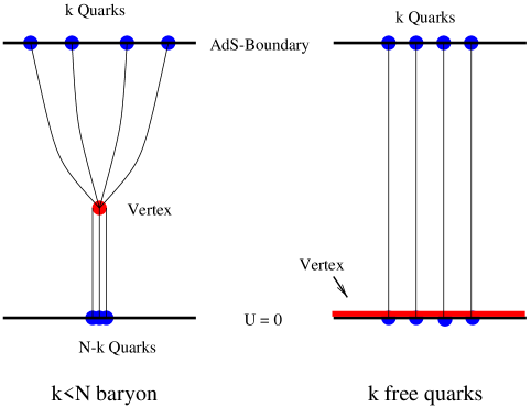
Figure 13: The $k<N$ “baryon” vs. $k$ free quarks. Since the longitudinal metric vanishes at $U=0$ the the surface $U=0$ is in fact a point and hence the vertex is smeared along this “surface” $U=0$. As a result the string can move freely at the boundary.

$$\frac{U_{x}}{\sqrt{U_{x}^{2}+U^{4}/R^{4}}}=A,~{}~{}~{}\mbox{where}~{}~{}~{}A=\frac{5N-4k}{4k}.$$ (86)

For $k=N$ we get $A=1/4$ and for $k<N$ we have $A>1/4$. It follows from (86) that $A\leq 1$. The upper bound , $A=1$ corresponds to $U_{x}\rightarrow\infty$ and $k=5N/8$. since the strings are radial the baryon size vanishes.

The energy of the k-quarks baryon is

$$E_{k}=\frac{U_{0}}{2\pi}\left[(N-k)+N/4+k\left(\int_{1}^{\infty}dy(\frac{y^{2}}{\sqrt{y^{4}-(1-A^{2})}}-1)-1\right)\right].$$ (87)

Where we have made the same kind of subtraction as in the $k=N$ configuration i.e. we have substracted the energy of $k$ quarks as depicted in fig.4b. For $A=1$ ($k=5N/8$) the energy vanishes which implies that the location of the D5-brane is a moduli of the system. For $A<1$ the energy is $bU_{0}$ with some negative $b$ and $U_{0}$ is determined, as usual, in terms of $L$.

Next we would like to analyze the non-supersymmetic case. As we remarked at the begging of this section, in a confining field theory we do not expect to find such states. This expectation seems to be supported by the AdS supergravity approach. The energy of a radial string is

$$E=\frac{1}{2\pi}\int_{U_{0}}^{U_{1}}dU\sqrt{G_{xx}G_{uu}}\sim\log(U_{0}-U_{T}).$$ (88)

Therefore, the energy of a string stretched between the D5-brane and the horizon is infinite and hence even the case $k=N-1$ cost an infinite amount of energy. Thus the baryonic configuration with $k=N$ is the only stable baryonic configuration with finite energy in agreement with field theory results.

Acknowledgements I would like to thank J. Labastida and J. Barbon for inviting me to present these lectures. The lectures are based on work done in collaboration with A. Armoni, A.Brandhuber,, E.Fuchs, N.Itzhaki, Y. Kinar, J. Maldacena, E. Schreiber, A Tseytlin, N. Weiss and S. Yankielowicz. I would like to thank them for the collaboration and for many useful discussions. This work is supported in part by the US-Israrel Binational Science Foundation, by GIF - the German-Israeli Foundation for Science Research, and by the Israel Science Foundation.

Note added While preparing these lecture notes the preprint [55] came out. In this work the contribution of the quantum fluctuations in the $AdS_{5}\times S^{5}$case is addressed in the framework of a Green Schwarz formulation. It is shon there that the partition function is well defined and finite. The BPS single quark, the circular loop and inifnite strip are annalyzed.

References

- [1] M. Luscher, K. Symanzik, P. Weisz, ”Anomalies of the free loop wave equation in the WKB approximation” Nucl. Phys. B173 (1980) 365.
- [2] O. Alvarez, Phys. Rev. D24 (1981) 440.
- [3] J. F. Arvis Phys. Lett. 127B (1983) 106.
- [4] J. M. Maldacena, “The Large N Limit of Superconformal Field Theories and Supergravity”, Adv.Theor.Math.Phys. 2 (1998) 231-252, hep-th/9711200.
- [5] S. S. Gubser, I. R. Klebanov and A. M. Polyakov, “Gauge Theory Correlators from Non-Critical String Theory”,Phys.Lett. B428 (1998) 105-114, hep-th/9802109.
- [6] E. Witten, “Anti De Sitter Space And Holography”, Adv. Theor. Math. Phys. 2 (1998) 253-291, hep-th/9802150.
- [7] O. Aharony, S. S. Gubser, J. Maldacena, H. Ooguri, Y. Oz “Large N Field Theories, String Theory and Gravity” hepth-9905111
- [8] J. Maldacena, ”Wilson loops in large field theories”, Phys. Rev. Lett. 80 (1998) 4859-4862, hep-th/9803002.
- [9] S.-J. Rey and J. Yee, “Macroscopic strings as heavy quarks in the large N gauge theory and anti-de Sitter supergravity”, hep-th/9803001.
- [10] D. Berenstein, R. Corrado, W. Fischler, J. Maldacena “ The Operator Product Expansion for Wilson Loops and Surfaces in the Large N Limit” Phys.Rev. D59 (1999) 105023 hep-th/9809188
- [11] N. Drukker, D. Gross and H. Ooguri ”Wilson Loops and Minimal Surfaces”, hep-th/9904191
- [12] E. Witten, ”Anti-de Sitter Space, Thermal Phase Transition, and Confinement in Gauge Theories”, hep-th/9803131.
- [13] A. Brandhuber, N. Itzhaki, J. Sonnenschein, S. Yankielowicz, ”Wilson Loops in the Large N Limit at Finite Temperature”, hep-th/9803137.
- [14] See the talk of D.Gross in this school.
- [15] S.J. Rey, S. Theisen and J.T. Yee, ”Wilson-Polyakov loop at finite Temperature in large gauge theory and anti-de Sitter supergravity”, hep-th/9803135.
- [16] A. Brandhuber, N. Itzhaki, J. Sonnenschein, S. Yankielowicz, ”Wilson Loops, Confinement, and Phase Transitions in Large N Gauge Theories from Supergravity”, JHEP 9806 (1998) 001,hep-th/9803263
- [17] D. Gross and H. Ooguri “Aspects of Large N Gauge Theory Dynamics as Seen by String Theory” Phys.Rev. D58 (1998) 106002, hep-th/9805129
- [18] Y. Kinar, E. Schreiber, J. Sonnenschein, ”Precision ’Measurements’ of the Potential in MQCD”, hep-th/9809133.
- [19] Y. Kinar, E. Schreiber and J. Sonnenschein, “ Potential from Strings in Curved Spacetime - Classical Results”, hep-th/9811192.
- [20] A.M. Polyakov, ”The Wall of the Cave”, hep-th/9809057.
- [21] I.R. Klebanov and A.A. Tseytlin, ”D-Branes and Dual Gauge Theories in Type 0 Strings”, hep-th/9811035.
- [22] J.A. Minahan, “Glueball Mass Spectra and Other Issues for Supergravity Duals of QCD Models”, hep-th/9811156.
- [23] I.R. Klebanov and A.A. Tseytlin, ”Asymptotic Freedom and Infrared Behavior in the Type 0 String Approach to Gauge Theory”, hep-th/9812089.
- [24] I.R. Klebanov and A.A. Tseytlin, ”A non-supersymmetric large N CFT from type 0 string theory”, hep-th/9901101.
- [25] Adi Armoni, E. Fuchs, J. Sonnenschein “Confinement in 4D Yang-Mills Theories from Non-Critical Type 0 String Theory” JHEP 9906 (1999) 027 hep-th/9903090
- [26] E. Witten, “Baryons and Branes in Anti-de Sitter Space”, hep-th/9805112.
- [27] A. Brandhuber, N. Itzhaki, J. Sonnenschein, S. Yankielowicz, “Baryons from supergravity”, JHEP 9807 (1998) 020 hep-th/9806158
- [28] Y. Imamura, “ Baryon Mass and Phase Transitions in Large N Gauge Theory” Prog.Theor.Phys. 100 (1998) 1263-1272 hep-th/9806162;
- [29] C. G. Callan, A. Guijosa, K. G. Savvidy, “ Baryons and Flux Tubes in Confining Gauge Theories from Brane Actions” Nucl.Phys. B555 (1999) 183-200 3. hep-th/9810092; “ Baryons and String Creation from the Fivebrane Worldvolume Action” Nucl.Phys. B547 (1999) 127-142
- [30] J. Sonnenschein, A. Loewy “ On the Supergravity Evaluation of Wilson Loop Correlators in Confining Theories” JHEP 0001 (2000) 042, hep-th/9911172
- [31] J. Greensite, P. Olesen, ”Remarks on the Heavy Quark Potential in the Supergravity Approach”, hep-th/9806235; ”Worldsheet Fluctuations and the Heavy Quark Potential in the AdS/CFT Approach”, hep-th/9901057.
- [32] H. Dorn and H.-J. Otto “On Wilson loops and -potentials from the AdS/CFT relation at ” hep-th/9812109;
- [33] H. Dorn, V. D. Pershin “ Concavity of the potential in super Yang-Mills gauge theory and AdS/CFT duality” hep-th/9906073
- [34] Y. Kinar, E. Schreiber, J. Sonnenschein, N.Weiss “Quantum fluctuations of Wilson loops from string models” hep-th/9911123
-
[35]
Ofer Aharony, Edward Witten
“ Anti-de Sitter Space and the Center of the Gauge Group”
JHEP 9811 (1998) 0181. hep-th/9807205
A. Volovich “Near Anti-de Sitter Geometry and Corrections to the Large N Wilson Loop” hep-th/9803220
E. Alvarez, C. Gomez, T. Ortin , “String Representation of Wilson Loops” Nucl.Phys. B545 (1999) 217-232, hep-th/9806075 A. Brandhuber, K. Sfetsos “ Wilson loops from multicentre and rotating branes, mass gaps and phase structure”, hep-th/9906201
K. Zarembo, “ Wilson Loop Correlator in the AdS/CFT Correspondence” Phys.Lett. B459 (1999) 527-534 hep-th/9904149 - [36] S. Kachru , E. Silverstein , “ 4d Conformal Field Theories and Strings on Orbifolds” hep-th/9802183 [abs, src, ps, other] : Phys.Rev.Lett. 80 (1998) 4855-4858
- [37] R. R. Metsaev, A. A. Tseytlin, ”Type IIB superstring action in background”, hep-th/9805028.
- [38] I. Pesando, ”A Gauge Fixed Type IIB Superstring Action on ”, hep-th/9808020.
- [39] R. Kalosh, J. Rahmfeld, ”The GS String Action on ”, hep-th/9808038.
- [40] R. Kallosh, A. A. Tseytlin, ”Simplifying Superstring Action on ”, hep-th/9808088.
- [41] M. Teper, ”Glueball masses and other physical properties of gauge theories in D=3+1”, hep-th/9812187.
- [42] L. Girardello, M. Petrini, M. Porrati and A. Zaffaroni, “Confinement and Condensates Without Fine Tuning in Supergravity Duals of Gauge Theories”, hep-th/9903026.
- [43] N. Itzhaki, J. Maldacena, J. Sonnenschein and S. Yankielowicz, ”Supergravity And The Large Limite Of Theories With Sixteen Supercharges”, hep-th/9802042.
- [44] C. Csáki, Y. Oz, J.Russo, J. Terning, ”Large QCD from Rotating Branes”, hep-th/9810186.
- [45] Hong Liu, A. A. Tseytlin “D3-brane - D-instanton configuration and N=4 super YM theory in constant self-dual background” Nucl.Phys. B553 (1999) 231-249,hep-th/9903091
- [46] M. Li, “’t Hooft Vortices on D-branes”, JHEP 9807 (1998) 003, hep-th/9803252.
- [47] R. R. Matsev and A. A. Tseytlin “Supersymmetric D3 brane action in ” Phys.Lett. B436 (1998) 281-288, hep-th/9806095
- [48] R. Kalosh and A. A. Tseytlin, “Simplifying superstring action on JHEP 9810 (1998) 016, hep-th/9808088
- [49] McKean and I. Singer J. Diff. Geom. 1 (1967) 43.
- [50] N. Graham, R. L. Jaffe Phys.Lett. B435 (1998) 145-151, hep-th/9805150, Nucl.Phys. B544 (1999) 432-447, hep-th/9808140; M. Shifman, A. Vainshtein, M. Voloshin, Phys.Rev. D59 (1999) 045016 hep-th/9810068; H., M. Stephanov, P. van Nieuwenhuizen, A. Rebhan Nucl.Phys. B542 (1999) 471-514 hep-th/9802074
- [51] S. Forste, D. Ghoshal and S. Theisen Stringy Corrections to the Wilson Loop in N=4 Super Yang-Mills Theory”, JHEP 9908 (1999) 013, hep-th/9903042 bibitemNaikS. Naik, “ Improved heavy quark potential at finite temperature from anti-de Sitter supergravity” Phys.Lett. B464 (1999) 73-76, hep-th/9904147
- [52] C. Bachas, Phys. Rv. D33 (1986) 2723.
- [53] C. Csaki, H. Ooguri, Y. Oz and J. Terning, “Glueball Mass Spectrum From Supergravity”, hep-th/9806021.
- [54] G. Horowitz and A. A. Tseytlin “A new class of exact solutions in string theory” hep-th 9409021
- [55] N. Drukker, D. J. Gross and A. A. Tseytlin “Green Schwarz string in semiclassical partition function” hep-th 0001204.
- [56] E. Witten, ”Branes And The Dynamics Of QCD”, Nucl.Phys. B507 (1997) 658-690, hep-th/9706109.
- [57] A.M. Polyakov, “String Theory and Quark Confinement”, Nucl. Phys. Proc. Suppl. 68 (1998) 1-8, hep-th/9711002.