Embedding Branes in Flat Two-time Spaces

Abstract:

We show how non-near horizon, non-dilatonic $p$-brane theories can be obtained from two embedding constraints in a flat higher dimensional space with 2 time directions. In particular this includes the construction of D3 branes from a flat 12-dimensional action, and M2 and M5 branes from 13 dimensions. The worldvolume actions are found in terms of fields defined in the embedding space, with the constraints enforced by Lagrange multipliers.

E mbedding geometric manifolds in higher dimensional flat spaces can be a useful tool for studying global properties of these manifolds. Typical examples of extending the dimension for a better understanding of the geometry are the description of the $d$-dimensional sphere $S^{d}$ by embedding it in $(d+1)$-dimensional Euclidean space and the description of $AdS_{d}$ as a hyperboloid in flat $(d+1)$-dimensional space with two timelike directions. The embedding is encoded, in both cases, in one constraint on the embedding coordinates and makes the $SO(p,q)$ global symmetry of these geometries manifest. Any choice of coordinates on the $d$-dimensional manifold will break this manifest symmetry.

The two examples above are combined in [1], where the $AdS_{p+2}\times S^{n-1}$ near-horizon geometry of $p$ branes in $D=p+n+1$ dimensions is described starting from a flat $(D+2)$-dimensional space. Two constraints are imposed, which respectively reduce $p+3$ dimensions to the $AdS_{p+2}$ manifold and $n$ dimensions to the $S^{n-1}$ sphere. The Born–Infeld action for the near-horizon theories of these branes can then be expressed in terms of $(D+2)$-dimensional fields, while the embedding constraints are imposed by means of Lagrange multipliers. The Wess–Zumino (WZ) terms in these actions can be obtained from a constant $(p+2)$ form in $D+2$ dimensions, which must be integrated over a $(p+2)$-dimensional manifold which has the worldvolume as its boundary.

This talk is based on the paper [2]. We will show, following [2], how the full spacetime metric of a brane can be embedded isometrically in ${{{\rm I\kern-1.79993ptE}}}^{D,2}$. In this way we generalize the construction of [1] to not just near-horizon, but to the full brane geometry. We will show that even if the geometry is not a product of $AdS$ times a sphere, the brane geometry can still be embedded in flat $(D+2)$-dimensional space with signature $(D,2)$. The two constraints are no longer independent in the sense that they do not constrain separate coordinates of the embedding space, but instead a non-trivial mixing of the coordinates is involved.

As in [1], also the forms for the WZ terms are obtained in this picture. For that construction, we will assume [3] that a $p$ brane evolving in a space with two times couples to a $(p+3)$-form field strength. The field strength is then contracted to a $(p+2)$-form which can be used for the WZ term. To make this contraction we will have to introduce an extra vector field which only in the near-horizon limit will have an elegant form.

One may wonder whether the whole geometry cannot be embedded with just one extra dimension and why we need two timelike directions for the embedding space. First of all, it has been shown [4] that the embedding of a surface in a flat space of co-dimension 1 imposes, by use of the Einstein equations, that the surface has constant curvature (if the surface has dimensionality $d>2$). This corresponds to familiar cases as the embedding of spheres and (anti–)de Sitter in flat spaces. Therefore, in order to embed brane backgrounds, which do not have constant curvature, we need at least two extra dimensions.

To determine the signature of the embedding space we use the following argument. An interesting aspect of brane spacetimes is that they are not globally hyperbolic. According to Penrose [5], a global isometric embedding in normal flat Minkowski space, i.e. in ${{{\rm I\kern-1.79993ptE}}}^{n,1}$, is only possible for a spacetime which is globally hyperbolic. Penrose’s argument is essentially that the restriction of the time coordinate $X^{0}$ of ${{{\rm I\kern-1.79993ptE}}}^{n,1}$ to the embedded spacetime $M$ would serve as a time-function on $M$, i.e., a function which increases along every future directed timelike curve. Moreover, if the embedding is suitably regular, the level sets (constant time slices) would actually serve as Cauchy surfaces on $M$, implying global hyperbolicity. In a sense any embedded surface inherits global hyperbolicity from the ambient space. No such obstruction arises for embeddings in flat space with more than one timelike direction. We will describe therefore a minimal embedding of general brane backgrounds in flat spaces with two extra dimensions and $(D,2)$ signature.

In section 1 we give the embedding of the geometry, commenting on global properties and on the near-horizon approximation. The worldvolume actions will be constructed in section 2. The essential step in that section is the construction of the forms. General results for the electric field strengths are given, before completing the construction for the example of the D3-brane.

1 Embedding: The geometry

In this section we describe the embedding of a $SO(n)$ invariant $p$-brane in a $(D+2)=(n+p+3)$-dimensional spacetime. We will obtain the embedding by requiring that the known metric of the brane is obtained from a flat $(D,2)$ metric, i.e. we demand that the embedding is isometric [6, 7]. The $D$-dimensional $p$-brane geometry can generally be described by a metric of the form

$$ds^{2} = A(r)^{2}\left[-dt^{2}+dx_{p}\cdot dx_{p}\right]+$$ (1)

$$+B(r)^{2}dr^{2}+C(r)^{2}d\Omega_{n-1}^{2}\,,$$

where $dx_{p}\cdot dx_{p}$ is the $p$-dimensional spacelike part of the worldvolume, and $d\Omega_{n-1}^{2}$ is the metric for the $n$-sphere.

On the embedding space ${{\rm I\kern-1.79993ptE}}^{(D,2)}$ we take cartesian coordinates $X^{M}$, with $M=0,\ldots,D+1$, which we divide as $X^{M}=(X^{\mu},X^{p+1},X^{p+2},X^{\alpha})$ (with $\mu=0,\ldots,p$, $\alpha=p+3,\ldots,D+1$). Using these coordinates, the metric looks as follows

$$ds^{2} = -(dX^{0})^{2}+(dX^{1})^{2}+\ldots+(dX^{p+1})^{2}+$$ (2)

$$-(dX^{p+2})^{2}+\ldots+(dX^{D+1})^{2}\,.$$

To obtain the two embedding constraints, we start by making a change of the $(D+2)$-dimensional coordinates, such that we make a subgroup $SO(p,1)\times SO(n)\subset SO(p+n+1,2)$ manifest. This is achieved by using a mixture of hyperspherical and horospherical coordinates $\{\rho,z,x^{\mu},\beta,n^{\alpha}\}$

$$X^{-}\equiv X^{p+2}-X^{p+1}=\frac{\rho}{z},$$

$$X^{+}\equiv X^{p+2}+X^{p+1}=\rho z+\frac{\rho}{z}x^{\mu}x_{\mu},$$

$$X^{\mu}=\rho\frac{x^{\mu}}{z}\,,\quad X^{\alpha}=\beta n^{\alpha}\,,$$ (3)

where $n^{\alpha}$ ($\sum_{\alpha}(n^{\alpha})^{2}=1$) parametrise the sphere $S^{n-1}$. In these new coordinates, the metric reads

$$ds^{2}=\frac{\rho^{2}}{z^{2}}\left[dx^{\mu}dx_{\mu}+dz^{2}\right]-d\rho^{2}+d\beta^{2}+\beta^{2}dn^{\alpha}dn^{\alpha}\,.$$ (4)

Comparing (4) and (1) we identify $dx^{\mu}dx_{\mu}$ with $-dt^{2}+dx_{p}.dx_{p}$ and $dn^{\alpha}dn^{\alpha}$ with $d\Omega_{n-1}^{2}$. Then $\beta$, $\rho$ and $z$ are functions of $r$ and are still to be determined. The comparison gives

$$\beta=C(r)\,,\quad\frac{\rho}{z}=A(r)\,,$$

$$-d\rho^{2}+\frac{\rho^{2}}{z^{2}}dz^{2}+d\beta^{2}=B(r)^{2}dr^{2}\,.$$ (5)

The differential equation can be rewritten to give

$$\frac{C^{\prime 2}-B^{2}}{A^{\prime}}=(\rho z)^{\prime}\equiv F^{\prime}\,.$$ (6)

From all this we can derive the following embedding functions

$$X^{-} = A(r)\,,\quad X^{+}=F(r)+A(r)x^{\mu}x_{\mu}$$

$$X^{\mu} = A(r)x^{\mu}\,,\quad X^{\alpha}=C(r)n^{\alpha}\,.$$ (7)

We can, furthermore, express the constraints in terms of the $X^{M}$ coordinates only. Denoting the inverse function with an overbar, i.e., $\bar{f}(f)=f(\bar{f})=\mathord{\!\leavevmode\hbox{ \begin{picture}(0.6,0.7)\put(0.0,0.0){\line(1,0){0.5}} \put(0.15,0.0){\line(0,1){0.7}} \put(0.35,0.0){\line(0,1){0.8}} \put(0.3,0.8){\rule{0.5pt}{0.5pt}}\put(0.26,0.78){\rule{0.5pt}{0.5pt}}\put(0.22,0.76){\rule{0.5pt}{0.5pt}}\put(0.18,0.74){\rule{0.5pt}{0.5pt}}\put(0.14,0.72){\rule{0.5pt}{0.5pt}}\put(0.1,0.7){\rule{0.5pt}{0.5pt}}\put(0.06,0.68){\rule{0.5pt}{0.5pt}}\put(0.02,0.66){\rule{0.5pt}{0.5pt}}\put(-0.02,0.64){\rule{0.5pt}{0.5pt}}\put(-0.06,0.62){\rule{0.5pt}{0.5pt}}\put(-0.1,0.6){\rule{0.5pt}{0.5pt}}\put(-0.14,0.58){\rule{0.5pt}{0.5pt}} \end{picture}}}$, we can write $r=\bar{A}(X^{-})$. Thus, our two constraints are

$$\phi_{1} = X^{-}X^{+}-X^{\mu}X_{\mu}-X^{-}F(\bar{A}(X^{-}))=0$$

$$\phi_{2} = \sum_{\alpha}(X^{\alpha})^{2}-\left[C(\bar{A}(X^{-}))\right]^{2}=0\,.$$ (8)

These constraints are therefore determined by the functions $A$, $C$ and $F$. The latter is determined up to a constant by (6) in terms of $A$, $B$ and $C$.

Note that so far there is no definition of the radial variable $r$. We can use different parametrizations, e.g. it will turn out that in some cases it is useful to take $A$ or $C$ itself as the radial variable. In the standard brane cases, the functions $A$, $B$ and $C$ will take the form of some harmonic function to some power in the transverse space of the brane. We will further adopt the name $r$ for that transverse coordinate, use just the name $A$ for the parameter in the first mentioned parametrization, and use $R$ for the radial coordinate such that $C(R)=R$.

From now on we will assume that the functions $A$, $B$ and $C$ are indeed harmonic functions in $n$ dimensions with a flat limit at $r\rightarrow\infty$. For non-dilatonic D- and M-branes, they are of the following form

$$H=\left(1+\frac{1}{r^{\kappa}}\right)\,,\quad A(r)=H^{-\frac{1}{p+1}}$$

$$B(r)=H^{\frac{1}{\kappa}}\,,\quad C(r)=rH^{\frac{1}{\kappa}}$$ (9)

where $\kappa\equiv n-2=D-p-3$. Here a priori $r>0$ and $r=0$ corresponds to the horizon, but we will come back to this later.

With this explicit form for the functions $A$, $B$ and $C$ we can evaluate the function $F$. Using (6) we get

$$F^{\prime}(r)=-wr^{1-\kappa}(1+r^{-\kappa})^{\frac{2}{\kappa}+\frac{1}{p+1}-1}(1+2r^{\kappa})\,,$$ (10)

(where $w=\frac{p+1}{\kappa}$), which can be integrated to give (up to a constant)

$$F(r) = -{\textstyle{w\over\kappa}}\left[B_{\frac{r^{\kappa}}{r^{\kappa}+1}}\left({\textstyle{-1\over p+1}},1-{\textstyle{2\over\kappa}}\right)\right.+$$ (11)

$$\left.+2B_{\frac{r^{\kappa}}{r^{\kappa}+1}}\left({\textstyle{p\over p+1}},-{\textstyle{2\over\kappa}}\right)\right]\,.$$

Here we used the incomplete Beta function

$$B_{x}(a,b) = \int_{0}^{x}t^{a-1}(1-t)^{b-1}dt=$$

$$= a^{-1}x^{a}{}_{2}F_{1}(a,1-b;a+1;x)\,,$$

which is defined for $0<x\leq 1$. This means that $F(r)$ is well defined in the region $r>0$, which is what we were looking for.

Note that near the horizon ($r\to 0$), where the brane geometry is well described by $AdS_{p+2}\times S_{D-p-2}$ [8], we get $F\sim w^{2}r^{-\frac{1}{w}}$ and the embedding functions (7) reduce to those used in [1].

Using the embedding (7) we can now study the global properties of the brane geometries. Before considering the higher dimensional D- and M-branes, let us first look at the simpler example of the extreme Reissner–Nordstrøm (RN) black hole. (A large list of embedding functions for other solutions of General Relativity is given in [9]). The RN black hole fits our general embedding scheme with $D=4$ and $p=0$, $\kappa=1$, $w=1$. Here, rather than working with the radial variable $r$ as in (9), we use the variable $R\equiv r+1$, which has the property $C(R)=R$. Then the functions $A$ and $B$ are given by $A(R)=B(R)^{-1}=1-1/R$. The horizon is now at $R=1$ and $R=0$ corresponds to the singularity. Using (6), we then find

$$F_{RN}(R)=\frac{1}{R-1}-3R-R^{2}-4\log|R-1|\,.$$

The entire Reissner–Nordstrøm black hole geometry can be drawn using parametrization (7) as is shown in figure 1. We only draw the relevant directions ($X^{-}$, $X^{+}$, and $X^{0}$), which basically means we only draw the $R$ and $t$ coordinates of the black hole (every point in the graph should be thought of as a 2-sphere). The lines in the graph are therefore constant $t$ and constant $R$ lines.

We can read off the following global features from the picture. The geometry consists of 2 distinct regions: region I, the asymptotically flat region for $R>1$ which corresponds to $X^{-}>0$. For big $R$ the surface flattens and $X^{-}\to 1$, which is the flat limit. Region II is the region inside the horizon ($X^{-}<0$), the singularity ($R=0$) corresponds to $X^{-}\to-\infty$. This is the global picture we recognize from the familiar Penrose diagram for extreme RN black hole as can be found in [2].

The two regions are connected in an $AdS$-throat. It seems that these two regions are disconnected, the constant time lines all diverge near $X^{-}=0$ and never cross the horizon, but this is just an artifact of the parametrization. Actually, we know that the near-horizon geometry is equivalent to $AdS_{2}$, which is known to have no problems at its ’horizon’. Indeed, a different parametrization exists (the advanced or retarded Finkelstein coordinates) in which lightlike geodesics pass smoothly through the horizon into the interior region, as is depicted in figure 2.

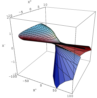
Figure 1: Extreme Reissner–Nordstrøm black hole parametrised by $R$ and $t$.

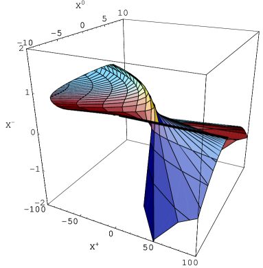
Figure 2: Extreme Reissner–Nordstrøm black hole in advanced Finkelstein coordinates $R$ and $v$ (with $v=t-R^{*}$, where $R^{*}=\int\frac{B(R)}{A(R)}dR$). The thick horizontal line is the horizon $R=1$.

One of the features of $AdS$ spaces is that they admit closed timelike curves. The usual remedy for this is to consider the covering space $CAdS$ instead of $AdS$ itself. Looking at figures 1 and 2 we see that the RN black hole geometry suffers from the same problem, it admits closed timelike curves. Again this is remedied by considering the covering space. The result of this of course is that the space then consists of multiple universes.

Let us now move to the non-dilatonic branes. As discussed in [10], the general brane solution case (9) can be divided in two classes: $p$ odd or $p$ even, with quite different global properties.

Let us first consider the $p$ odd case. In the exterior region ($r>0$), the function $A(r)$ is analytic and positive and vanishes as $r\to 0$. If we take $A$ to be our new radial variable instead of $r$, we see that $A$ can be continued through the horizon to negative $A$ [10]. The range of $A$ is from -1 to 1. The analytic extension of the metric is

$$ds^{2}=A^{2}dx_{\mu}dx^{\mu}+\left(1-A^{p+1}\right)^{-\frac{2}{\kappa}}\times$$ (12)

$$\times \left[w^{2}\left(1-A^{p+1}\right)^{-2}A^{-2}dA^{2}+d\Omega^{2}\right]\,,$$

which is even in $A$. This leads to

$$F(A) = -{\textstyle{w\over\kappa}}(\mbox{sign }A)\bigl{[}B_{A^{p+1}}\left({\textstyle{-1\over p+1}},1-{\textstyle{2\over\kappa}}\right)+$$ (13)

$$+B_{A^{p+1}}\left({\textstyle{p\over p+1}},-{\textstyle{2\over\kappa}}\right)\bigr{]}\,.$$

The embedding functions (7) are then odd in $A$. This means that the embedded space is symmetric around the horizon and completely nonsingular. For the non-dilatonic branes, the D3 and M5 fit this picture. The embedding, depicted in figure 3 for the D3-brane case, nicely shows these features (an analogous picture for the M5-brane can be found in [2]). It is clearly visible there is no interior region, just two symmetric ’exterior’ regions connected in the AdS-throat as was expected from the Penrose diagram [10] [2].

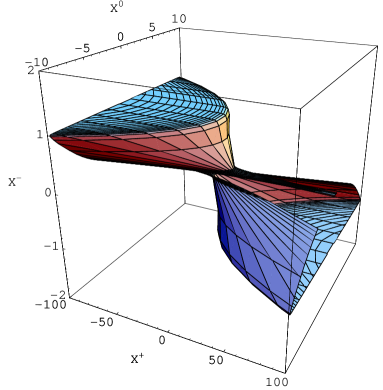
Figure 3: $p$ odd branes (D3). Two asymptotically flat regions connected in AdS.

In the $p$ even case, the metric and embedding functions are neither even nor odd. It is useful in this case to adopt so-called Schwarzschild coordinates, defined by $R^{\kappa}=r^{\kappa}+1$. In these coordinates the horizon (which is still a coordinate singularity) is at $R=1$. At $R=0$ there is a true curvature singularity. Expressed in this coordinate, $A(R)$ can be continued through the horizon into negative $A$ and its range is $\{-\infty,1\}$. As already stated in [10], the Penrose diagram for these spaces is equivalent to the extreme Reissner–Nordstrøm diagram.

The embedding of the M2-brane metric illustrates these features. The expression (11) of $F$ is only well defined in the region $R>1$. It is not possible to find a continuous expression for $F$ valid in both regions ($0<R\leq 1$ and $R>1$). But, nevertheless, a continuous embedding is obtained using in the interior region

$$F(R<1) = {\textstyle{w\over\kappa}}\bigr{[}B_{R^{\kappa}}\left({\textstyle{1\over p+1}}+{\textstyle{2\over\kappa}},-{\textstyle{1\over p+1}}\right)+$$

$$-2B_{R^{\kappa}}\left({\textstyle{1\over p+1}}+{\textstyle{3\over\kappa}},-{\textstyle{1\over p+1}}\right)\bigr{]}\,.$$

The global properties of the M2-brane are qualitatively the same as those of the RN black hole depicted in figure 1. We refer to [2] for the M2-picture.

2 The brane action

We would like to write the action of a brane placed in the background of other branes using the embedding of the previous section. A typical (schematic) form of the action is

$$S_{p+1} = \int_{W}d^{p+1}\xi\sqrt{-\det{\cal G}_{\mu\nu}}+\int_{B}\Omega_{(p+2)}+$$ (14)

$$+\int_{W}d^{p+1}\xi[\lambda_{1}\phi_{1}+\lambda_{2}\phi_{2}]\,,$$

where $W=\partial B$ is the $(p+1)$-dimensional world volume of the brane. The expression for ${\cal G}_{\mu\nu}$ differs in each case. For example, for Dp-branes ${\cal G}_{\mu\nu}\equiv\partial_{\mu}X^{M}\partial_{\nu}X^{N}\eta_{MN}+{\cal F}_{\mu\nu}$, with ${\cal F}_{\mu\nu}$ the field strength of the gauge field living on the world volume of the brane. The fields $\lambda_{1},\lambda_{2}$ are two Lagrange multipliers implementing the constraints (8). $\Omega_{(p+2)}(X^{M})$ is a function of the forms coupling to the brane, such that it reduces to the appropriate Wess–Zumino term when projected onto the physical hypersurface. Its explicit form will be determined for the D3-brane case in section 2.2. An analogous treatment for M2 and M5 is given in [2].

2.1 Embedding the field strength

Let us now try to embed the field strengths appearing in the Wess–Zumino term. We will assume [3] that a brane (extended in $p$ spatial directions) fluctuating in a spacetime with two times should evolve in both time directions, and therefore couple to a (p+3)-form field strength. We assume therefore that the $(D+2)$-dimensional theory can be coupled to a rank $p+3$ electric field strength $K_{e}$, and to a rank $n$ magnetic field strength $K_{m}$.

This ansatz is the most natural one for the D3-brane, because in this case the $10$-dimensional self-dual field strength is extended to a self-dual field strength in $12$ dimensions. If there would be a supergravity theory in $D=12$, the bosonic configuration with flat $(10,2)$ space and a constant self-dual field strength would solve the equations of motion. This is obvious for the Maxwell equation (there can be no Chern–Simons terms built from a 5 form potential in 12 dimensions and so the Maxwell equation would take the standard form), but for the Einstein equations it is only true because the field strength is self-dual. In a $D$-dimensional spacetime with zero or two times, a self-dual field strength has a vanishing energy momentum tensor for $D=4$ mod 4. (For Lorentzian signature it is $D=2$ mod 4). What this would mean is that the ten-dimensional D3-brane solution would just be the projection to a complicated hypersurface of an almost trivial 12 dimensional supergravity solution.

Let us start by analysing how an electric $(p+2)$-form field strength $F^{(p+2)}$ gets embedded in the $(D+2)$-dimensional space. Our aim is to obtain $F$ as a restriction of a $p+3$-form $K^{(p+3)}$ to the $D$-dimensional hypersurface $\Sigma$. A general non-dilatonic brane is described in $D$ dimensions by the fields [11]

$$ds^{2} = H^{-\frac{2}{p+1}}\left[-dt^{2}+dx_{1}^{2}+\cdots+dx_{p}^{2}\right]+$$

$$+H^{\frac{2}{\kappa}}\left[dr^{2}+r^{2}d\Omega_{D-p-2}^{2}\right],$$

$$G_{01...p} = -H^{-1}=-A^{p+1},$$

$$\Phi = 0\,,$$ (15)

using the notation of section 1. We can write the (electric) field strength as ($F\equiv dG$)

$$F=-(p+1)A^{p}A^{\prime}dr\wedge dt\wedge dx_{1}\wedge\cdots\wedge dx_{p}\,,$$ (16)

where the prime denotes differentiation with respect to $r$.

To find the embedding, we start by considering a constant $(p+3)$-form in $D+2$ dimensions

$$K_{e}=\frac{p+1}{(p+3)!}\epsilon_{\mu^{\prime}_{0}...\mu^{\prime}_{p+2}}dX^{\mu^{\prime}_{0}}\wedge dX^{\mu^{\prime}_{1}}...\wedge dX^{\mu^{\prime}_{p+2}}$$ (17)

($\mu^{\prime}=0,\ldots,p+2$). In order to get a rank $(p+2)$ field strength, we contract $K_{e}$ with a vector field $V$, with components $V=V^{M}(\frac{\partial}{\partial X^{M}}$), which so far remains arbitrary. (There is a sign ambiguity in this contraction; we chose to make it on the left, i.e. $K(V)_{\mu^{\prime}_{1}...\mu^{\prime}_{p+2}}\equiv V^{\mu^{\prime}_{0}}K_{\mu^{\prime}_{0}...\mu^{\prime}_{p+2}}$). Such a contraction yields

$$K_{e}(V)=\frac{p+1}{(p+2)!}\epsilon_{\mu^{\prime}_{0}...\mu^{\prime}_{p+2}}V^{\mu^{\prime}_{0}}dX^{\mu^{\prime}_{1}}\wedge...dX^{\mu^{\prime}_{p+2}}\,.$$ (18)

Then we reduce the resulting $(p+2)$-form to the $D$ dimensional hypersurface by using the embedding functions (7),

$$K_{e}(V)|_{\Sigma}=\frac{p+1}{2}A^{\prime}A^{p+1}dr\wedge dt\wedge dx_{1}\wedge\cdots dx_{p}\times$$

$$\times\left[2V^{\mu}x_{\mu}+V^{+}(\frac{F^{\prime}}{A^{\prime}}-x^{\mu}x_{\mu})-V^{-}\right]\,,$$ (19)

where we defined $V^{\pm}\equiv V^{p+2}\pm V^{p+1}$. Next we impose that $K_{e}(V)|_{\Sigma}=F$. From this we can determine $V^{M}$, using the ansatz $V^{\mu^{\prime}}=\alpha(r)X^{\mu^{\prime}}$. Because $K_{e}$ only has components in the longitudinal directions, $V^{\alpha}$ stays undetermined. When the field strength also includes a magnetic part, this $V^{\alpha}$ comes into play, as we will see in the next subsection. It follows that, in order for (19) to match with (16), $\alpha(r)$ has to obey

$$\alpha(r)(\frac{AF^{\prime}}{A^{\prime}}-F)=-\frac{2}{A}$$ (20)

which gives, using (6)

$$\alpha(r)=\frac{2}{AF+w^{2}C^{2}(2C^{\kappa}-1)}\,.$$ (21)

or, in terms of the embedding coordinates ($\alpha(r)\to\alpha(r(X))\equiv\alpha(X)$)

$$\alpha(X)=\frac{2}{w^{2}(X_{\alpha})^{2}\left[2(X_{\alpha})^{\kappa}-1+w^{-2}\right]-(X_{M})^{2}}$$ (22)

and $V^{\mu^{\prime}}(X)=\alpha(X)X^{\mu^{\prime}}$.

2.2 D3-brane embedding

Let us now discuss, as an example, how this construction works for the D3-brane in the background produced by other D3-branes. We refer to [2] for a discussion of the embedding of the M2- and M5-brane.

The 10-dimensional Wess–Zumino term is the integral of the self-dual field strength $F$ that couples to the D3-branes solution of the type IIB supergravity theory. For the 12-dimensional theory we construct a self-dual 6 form $K$, i.e.

$$\star{K}\wedge K=\eta_{12}|K|^{2},$$ (23)

where $\eta_{12}$ is the volume form on ${{\rm I\kern-1.79993ptE}}^{(D,2)}$. Our aim is to obtain $F$ as a restriction of $K$ to the 10 dimensional surface $\Sigma$. The D3-brane is described by the fields (15) with $p+1=\kappa=4$, $D=10$. We can therefore write the self-dual field strength in terms of the embedding functions as

$$F=-4A^{\prime}A^{3}dt\wedge dx\wedge dy\wedge dz\wedge dr+4\omega_{(5)}\,,$$ (24)

where $\omega_{(5)}\equiv\sin(\theta)^{4}\sin(\phi_{1})^{3}\sin(\phi_{2})^{2}\sin(\phi_{3})d\theta\wedge d\phi_{1}\wedge...\wedge d\phi_{4}$ is the volume form on the unit 5-sphere.

To find the embedding, we again start by considering a constant form in the embedding space, which in this case we take to be a self-dual six-form

$$K = \frac{4}{6!}(\epsilon_{\mu^{\prime}_{0}...\mu^{\prime}_{5}}dX^{\mu^{\prime}_{0}}\wedge dX^{\mu^{\prime}_{1}}...\wedge dX^{\mu^{\prime}_{5}}+$$ (25)

$$+ \epsilon_{\alpha_{1}...\alpha_{6}}dX^{\alpha_{1}}\wedge dX^{\alpha_{1}}...\wedge dX^{\alpha_{6}}),$$

In order to get a rank 5 field strength, we contract, as we have done for the general electric case, $K$ with a vector field $V$. Such a contraction yields

$$K(V) = \frac{4}{5!}(\epsilon_{\mu^{\prime}_{0}...\mu^{\prime}_{5}}V^{\mu^{\prime}_{0}}dX^{\mu^{\prime}_{1}}\wedge...\wedge dX^{\mu^{\prime}_{5}}+$$ (26)

$$+ \epsilon_{\alpha_{1}...\alpha_{6}}V^{\alpha_{1}}dX^{\alpha_{2}}\wedge...\wedge dX^{\alpha_{6}})\,.$$

Again we reduce the resulting 5 form to the 10-dimensional hypersurface by using the embedding functions (7). By requiring the matching $K(V)|_{\Sigma}=F$, we get the constraints on our vector field $V$. The resulting 5 form $K(V)|_{\Sigma}$ is precisely the Wess–Zumino term $\Omega_{5}$ we were looking for.

Let us analyse separately the two terms in the right hand side of (24), (25) and (26). The electric part has already been studied in the general case in the previous subsection. In this case it gives $V^{\mu^{\prime}}=\alpha(r)X^{\mu^{\prime}}$ with

$$\alpha(X)=\frac{2}{2(X^{\alpha}X_{\alpha})^{3}-X^{M}X_{M}}\,.$$ (27)

The magnetic part in (25) can be rewritten in terms of the radial coordinate $r$ and the angular coordinates $\theta$,$\phi_{i}$ ($i=1,\cdots,4$)

$$\frac{1}{6!}\epsilon_{\alpha_{1}...\alpha_{6}}dX^{\alpha_{1}}\wedge\cdots\wedge dX^{\alpha_{6}}=$$

$$\quad\quad=C^{\prime}C^{5}dr\wedge\omega_{5}\,.$$ (28)

For the second term in (26) to match with the second term in (24), we have to require that the vector $V^{\alpha}$ points in the radial direction when decomposed in the $r,\theta,\phi_{i}$ basis, that is

$$V^{\alpha}\frac{\partial}{\partial X^{\alpha}}\equiv V^{\alpha}\frac{\partial r}{\partial X^{\alpha}}\frac{\partial}{\partial r}\,.$$ (29)

This gives

$${\textstyle{1\over 5!}}\epsilon_{\alpha_{1}...\alpha_{6}}V^{\alpha_{1}}dX^{\alpha_{2}}\wedge...\wedge dX^{\alpha_{6}}=$$

$$\quad\quad=C^{\prime}C^{5}V^{\alpha}\frac{\partial r}{\partial X^{\alpha}}\omega_{5}\,.$$ (30)

Matching this with (24) requires

$$V^{\alpha}\frac{\partial r}{\partial X^{\alpha}}=(C^{\prime}C^{5})^{-1}\,,$$ (31)

which, using the ansatz $V^{\alpha}=\epsilon(r)X^{\alpha}$, is solved by

$$V^{\alpha}=C^{-6}X^{\alpha}=(1+r^{4})^{-\frac{3}{2}}X^{\alpha}\,.$$ (32)

We notice that $\epsilon(r\to 0)=\alpha(r\to 0)\to 1$, so that in the near-horizon approximation we have $V^{M}=X^{M}$ as was already found in [1].

The general form of the vector field in terms of the 12-dimensional coordinates is

$$V^{\mu^{\prime}}=\frac{2X^{\mu^{\prime}}}{2(X^{\alpha}X_{\alpha})^{3}-X^{M}X_{M}},\,V^{\alpha}=\frac{X^{\alpha}}{(X^{\beta}X_{\beta})^{3}}\,.$$ (33)

3 Discussion

The aim of this talk has been to report on a global description [2] of non-dilatonic branes by isometrically embedding them in flat space with two extra dimensions and two times, thus extending the ideas of [1]. We have gained a rather clear global picture of the geometry, giving insight in the structure around coordinate singularities and in the symmetries. In particular, the differences between $p$-branes with $p$ even and $p$ odd, previously pointed out in [10], are clearly apparent. Like the familiar embedding of anti-de Sitter spacetime as a quadric, our embeddings are periodic in time. This is consistent with some suggestions in [12], but one may of course always pass to the covering space.

In the context of supergravity and string theory, $p$-branes are coupled to $(p+2)$-form field strengths. An embedding of the brane thus has to include, besides the embedding of the geometry, a prescription for the forms in the higher dimensional space. This is obtained by defining constant $(p+3)$-forms in $D+2$ dimensions, and contracting them using a vector $V$. The form of $V$ is determined by matching the projection on the surface with the known forms for the branes field strengths.

Unfortunately, the geometric significance of the vector field $V$ remains unclear. In the case of the M2-brane it is not even unique, since the $V^{\alpha}$ components are arbitrary. A co-dimension 2 surface has a 2-dimensional normal plane. In the D3 and M5 cases, the vector $V$ does not lie in this 2-plane, except in the near-horizon limit. Specifically, the normal 2-plane is spanned by $\partial_{\mu}\phi_{1}$ and $\partial_{\mu}\phi_{2}$. One may check that $V$ is not a linear combination of $\partial_{\mu}\phi_{1}$ and $\partial_{\mu}\phi_{2}$. The bosonic action for probe branes in the embedded background (14) is completely determined after the construction of $V$. It could be interesting to investigate if the vector $V$ can have some role in the context of F-theory [13].

Finally it is possible that the methods developed in this paper may be applicable to scenarios in which one regards the universe as a brane embedded in a higher-dimensional spacetime.

References

- [1] P. Claus, R. Kallosh, J. Kumar, P.K. Townsend and A. Van Proeyen, J. High Energy Phys. 06 (1998) 004 ; hep-th/9801206.
- [2] L. Andrianopoli, M. Derix, G.W. Gibbons, C. Herdeiro, A. Santambrogio and A. Van Proeyen, Isometric Embedding of BPS Branes in Flat Spaces with Two Times, hep-th/9912049
- [3] S.F. Hewson, An approach to F-theory, hep-th/9712017.
- [4] L.P. Eisenhart, Riemannian Geometry, Princeton university press Princeton (N.J.) (1997) 306 p.
- [5] R. Penrose, A remarkable property of plane waves in General Relativity, Rev. Mod. Phys. 37 N. 1 (1965) 215.
- [6] H.Goenner, Local Isometric embeddings of Riemannian Manifolds and Einstein’s Theory of Gravitation, in “General Relativity and Gravitation: One hundred years after the birth of Einstein”, Edited by A.Held, Vol.1.
- [7] A.Friedman, Isometric Embeddings of Riemannian manifolds into Euclidean spaces, Rev. Mod. Phys. 37 (1965) 201.
- [8] G.Gibbons, P.Townsend, Vacuum interpolation in supergravity via super p-branes, Phys. Rev. Lett. 71 (1993) 3754; hep-th/9307049.
- [9] J.Rosen, Embedding various relativistic Riemannian spaces in Pseudo Euclidean spaces, Rev. Mod. Phys. 37 (1965) 204.
- [10] G.W. Gibbons, G.T. Horowitz and P.K. Townsend, Higher dimensional resolution of dilatonic black hole singularities, Class. and Quant. Grav. 12 (1995) 297, hep-th/9410073.
- [11] M.J.Duff and J.X.Lu, The self-dual type IIB superthreebrane, Phys. Lett. B 273 (1991) 409; for the M-branes see, for instance K.Stelle lectures on supergravity p-branes, hep-th/9701088.
- [12] G.W. Gibbons, Wrapping Branes in Space and Time, hep-th/9803206.
- [13] C. Vafa, Evidence for F-Theory, Nucl. Phys. B 469 (1996) 403.