Abstract

We describe consequences of the chiral anomaly in the theory of quantum wires, the (quantum) Hall effect, and of a four-dimensional cousin of the Hall effect. We explain which aspects of conductance quantization are related to the chiral anomaly. The four-dimensional analogue of the Hall effect involves the axion field, whose time derivative can be interpreted as a (space-time dependent) difference of chemical potentials of left-handed and right-handed charged fermions. Our four-dimensional analogue of the Hall effect may play a significant rôle in explaining the origin of large magnetic fields in the (early) universe.

1 What is the chiral anomaly?

The chiral abelian anomaly has been discovered, in the past century, by Adler, Bell and Jackiw, after earlier work on $\pi^{0}$-decay starting with Steinberger and Schwinger; see e.g. [1] and references given there. It has been rederived in many different ways of varying degree of mathematical rigor by many people. Diverse physical implications, especially in particle physics, have been discussed. It is hard to imagine that one may still be able to find new, interesting implications of the chiral anomaly that specialists have not been aware of, for many years. Yet, until very recently — in the past century, but only two to three years ago — this turned out to be possible, and we suspect that further applications may turn up in the future! This little review is devoted to a discussion of physical implications of the chiral anomaly that have been discovered recently.

Before we turn to physics, we recall what is meant by “chiral (abelian) anomaly”. In general terms, one speaks of an anomaly if some quantum theory violates a symmetry present at the classical level, (i.e., in the limit where $\hbar\to 0$). By “violating a symmetry” one means that it is impossible to construct a unitary representation of the symmetry transformations of the classical system underlying some quantum theory on the Hilbert space of pure state vectors of the quantum theory. (By “violating a dynamical symmetry” is meant that it is impossible to construct such a representation that commutes with the unitary time evolution of the quantum theory.)

It is quite clear that understanding anomalies can be viewed as a problem in group cohomology theory. A fundamental example of an anomalous symmetry group is the group of all symplectic transformations of the phase space of a classical Hamiltonian system underlying some quantum theory.

The anomalies considered in this review are ones connected with infinite-dimensional groups of gauge transformations which are symmetries of some classical Lagrangian systems with infinitely many degrees of freedom (Lagrangian field theories). Thus, we consider a theory of charged, massless fermions coupled to an external electromagnetic field in Minkowski space-time of even dimension $2n$. Let $\gamma^{0},\gamma^{1},\ldots,\gamma^{2n-1}$ denote the usual Dirac matrices, and define

$$\gamma\;:=\;i\,\gamma^{0}\,\gamma^{1}\ldots\gamma^{2n-1}\ .$$ (1.1)

Then $\gamma$ anti-commutes with the covariant Dirac operator

$$D\;:=\;i\,\gamma^{\mu}\,\left(\partial_{\mu}-iA_{\mu}\right)\ ,$$ (1.2)

where $A$ is the vector potential of the external electromagnetic field. Let $\psi(x)$ denote the Dirac spinor field and $\bar{\psi}(x)$ the conjugate field. We define the vector current, ${\mathcal{J}}^{\mu}$, and the axial vector current $\widetilde{{\mathcal{J}}}^{\mu}$, by

$${\mathcal{J}}^{\mu}\;:=\;\bar{\psi}\gamma^{\mu}\psi\ ,\ \widetilde{{\mathcal{J}}}^{\mu}\;:=\;\bar{\psi}\gamma^{\mu}\gamma\psi\ .$$ (1.3)

At the classical level, these currents are conserved,

$$\partial_{\mu}{\mathcal{J}}^{\mu}\;=\;0~{},~{}~{}\partial_{\mu}\widetilde{{\mathcal{J}}}^{\mu}\;=\;0~{},$$ (1.4)

on solutions of the equations of motion, $(D\psi=0)$. The conservation of the vector current is intimately connected with the electromagnetic gauge invariance of the theory,

$${}\psi(x)\mapsto e^{i\chi(x)}\psi(x)~{},~{}~{}\bar{\psi}(x)\mapsto\bar{\psi}(x)\;e^{-i\chi(x)}$$

$${}~{}~{}~{}~{}~{}~{}A_{\mu}(x)\mapsto A_{\mu}(x)+\partial_{\mu}\chi(x)~{},$$ (1.5)

where $\chi(x)$ is a test function on space-time. When $\chi$ is constant in $x$ the transformations (1.5) are a global symmetry of the classical theory corresponding to the conserved quantity

$$Q\;=\;\int d\underline{x}\;{\mathcal{J}}^{0}\left(x^{0},\underline{x}\right)$$ (1.6)

which is the electric charge. The conservation of $Q$ (independence of $x^{0}$) follows, of course, from the fact that the Noether current ${\mathcal{J}}^{\mu}$ associated with (1.5) satisfies the continuity equation (1.4).

The conservation of the axial vector current $\widetilde{{\mathcal{J}}}^{\mu}$, in the classical theory, is connected with the invariance of the theory under local chiral rotations

$${}\psi(x)\mapsto e^{i\alpha(x)\gamma}\psi(x),~{}~{}\bar{\psi}(x)\mapsto\bar{\psi}(x)\;e^{i\alpha(x)\gamma}$$

$${}~{}~{}~{}~{}~{}~{}~{}~{}~{}~{}~{}A_{\mu}(x)\mapsto A_{\mu}(x)+\gamma\partial_{\mu}\alpha(x)~{},$$ (1.7)

where $\alpha(x)$ is a test function on space-time. In particular, when $\alpha$ is a constant the transformations (1.7) are a global symmetry of the classical theory corresponding to the conserved charge

$$\widetilde{Q}\;=\;\int d\underline{x}\;\widetilde{{\mathcal{J}}}^{0}\left(x^{0},\underline{x}\right)$$ (1.8)

(which, according to (1.4), is independent of $x^{0}$).

It turns out that, in the quantum theory, the local chiral rotations (1.7) do not leave quantum-mechanical transition amplitudes invariant, and the axial vector current $\widetilde{{\mathcal{J}}}^{\mu}$ is not a conserved current, for arbitrary external electromagnetic fields. This phenomenon is called chiral (abelian) anomaly.

Let us see where the chiral anomaly comes from, for theories in two and four space-time dimensions. We start with the discussion of two-dimensional theories. We consider a quantum theory which has a conserved vector current ${\mathcal{J}}^{\mu}$ and — if the external electromagnetic field vanishes — a conserved axial vector current $\widetilde{{\mathcal{J}}}^{\mu}$, i.e.,

$$\partial_{\mu}\,{\mathcal{J}}^{\mu}\;=\;0~{},~{}~{}\partial_{\mu}\,\widetilde{{\mathcal{J}}}^{\mu}\;=\;0~{}.$$ (1.9)

In two space-time dimensions, ${\mathcal{J}}^{\mu}$ and $\widetilde{{\mathcal{J}}}^{\mu}$ are related to each other by

$$\widetilde{{\mathcal{J}}}^{\mu}\;=\;\varepsilon^{\mu\nu}\,{\mathcal{J}}_{\nu}$$ (1.10)

where $\varepsilon^{00}=\varepsilon^{11}=0~{},~{}~{}\varepsilon^{01}=-\varepsilon^{10}=1$. The continuity equation

$$\partial_{\mu}\,{\mathcal{J}}^{\mu}\;=\;0$$

has the general solution

$${\mathcal{J}}^{\mu}(x)\;=\;\frac{q}{2\pi}~{}\varepsilon^{\mu\nu}\left(\partial_{\nu}\,\varphi\right)(x)~{},$$ (1.11)

where $\varphi(x)$ is an arbitrary scalar field on space-time, and $q$ denotes the electric charge. Using eqs. (1.11) and (1.10) and the continuity equation,

$$\partial_{\mu}\,\widetilde{{\mathcal{J}}}^{\mu}\;=\;0~{},$$

for the axial vector current, we find that the field $\varphi$ must obey the equation of motion

$$\square~{}\varphi(x)\;=\;0~{}.$$ (1.12)

Thus, if the vector- and axial vector currents are conserved then the potential $\varphi$ of the vector current is a massless free field. The theory of the massless free field is an example of a Lagrangian field theory. It has an action functional, $S$, given by

$$S(\varphi)\;=\;\frac{1}{4\pi}\int d^{2}x\;\left(\partial_{\mu}\varphi\right)(x)\left(\partial^{\mu}\varphi\right)(x)~{}.$$ (1.13)

The “momentum”, $\pi(x)$, canonically conjugate to $\varphi(x)$ is defined, as usual, by

$$\pi(x)\;=\;\delta S(\varphi)\big{/}\delta\left(\partial_{0}\varphi(x)\right)\;=\;\frac{1}{2\pi}~{}\frac{\partial\varphi(x)}{\partial t}~{},$$ (1.14)

where $t=x^{0}$ denotes time; (the “velocity of light” $c=1$). In the quantum theory, $\varphi$ and $\pi$ are operator-valued distributions on Fock space satisfying the equal-time canonical commutation relations

$$\left[\pi\left(t,\underline{x}\right)~{},~{}~{}\varphi\left(t,\underline{y}\right)\right]\;=\;-i\delta\left(\underline{x}-\underline{y}\right)~{}.$$ (1.15)

Since

$${\mathcal{J}}^{\mu}(x)\;=\;\frac{q}{2\pi}~{}\varepsilon^{\mu\nu}\left(\partial_{\nu}\varphi\right)(x)~{},$$

and

$$\widetilde{{\mathcal{J}}}^{\mu}(x)\;=\;\varepsilon^{\mu\nu}{\mathcal{J}}_{\nu}(x)\;=\;\frac{q}{2\pi}~{}\left(\partial^{\mu}\varphi\right)(x)~{},$$

eq. (1.15) yields the well known anomalous commutator

$$\left[{\mathcal{J}}^{0}\left(t,\underline{x}\right)~{},~{}~{}\widetilde{{\mathcal{J}}}^{0}\left(t,\underline{y}\right)\right]\;=\;i~{}\frac{q^{2}}{2\pi}~{}\delta^{\prime}\left(\underline{x}-\underline{y}\right)~{}.$$ (1.16)

Next, we imagine that the system is coupled to a classical external electric field $E(x)$. In two space-time dimensions, the electric field is given in terms of the electromagnetic vector potential $A_{\mu}$ by

$$E(x)\;=\;\varepsilon^{\mu\nu}\left(\partial_{\mu}A_{\nu}\right)(x)~{}.$$ (1.17)

The action functional for the theory in an external electric field is given by

$$S\left(\varphi,A\right) = \frac{1}{4\pi}\int d^{2}x\left(\partial_{\mu}\varphi\right)(x)\left(\partial^{\mu}\varphi\right)(x)~{}+~{}\frac{1}{q}\int d^{2}x{\mathcal{J}}^{\mu}(x)A_{\mu}(x)$$ (1.18)

$$= \frac{1}{4\pi}\int d^{2}x\left\{\left(\partial_{\mu}\varphi\right)(x)\left(\partial^{\mu}\varphi\right)(x)~{}+~{}2\,\varepsilon^{\mu\nu}\partial_{\nu}\varphi(x)A_{\mu}(x)\right\}~{}.$$

The equation of motion (Euler-Lagrange equation) obtained from the action function (1.18) is

$$\square~{}\varphi(x)\;=\;E(x)~{}.$$ (1.19)

Using (1.10) and (1.11), we see that equation (1.19) is equivalent to

$$\partial_{\mu}\widetilde{{\mathcal{J}}}^{\mu}(x)\;=\;\frac{q}{2\pi}~{}E(x)~{},$$ (1.20)

i.e., the axial vector current fails to be conserved in a non-vanishing external electric field $E$. Equation (1.20) is the standard expression of the chiral anomaly in two space-time dimensions.

From the currents ${\mathcal{J}}^{\mu}$ and $\widetilde{{\mathcal{J}}}^{\mu}$ one can construct chiral currents, ${\mathcal{J}}_{\ell}^{\mu}$ and ${\mathcal{J}}_{r}^{\mu}$, for left-moving and right-moving modes by setting

$${\mathcal{J}}_{\ell}^{\mu}\;=\;{\mathcal{J}}^{\mu}-\widetilde{{\mathcal{J}}}^{\mu}~{},~{}~{}{\mathcal{J}}_{r}^{\mu}\;=\;{\mathcal{J}}^{\mu}+\widetilde{{\mathcal{J}}}^{\mu}~{}.$$ (1.21)

They satisfy the equations

$$\partial_{\mu}{\mathcal{J}}_{\ell/r}^{\mu}\;=\;\mp~{}\frac{q}{2\pi}~{}E(x)~{}.$$ (1.22)

From eqs. (1.17) and (1.22) we infer that one can define modified chiral currents, $\widehat{{\mathcal{J}}}_{\ell/r}^{\mu}$, which are conserved:

$$\widehat{{\mathcal{J}}}_{\ell/r}^{\mu}(x)\;:=\;{\mathcal{J}}_{\ell/r}^{\mu}\;\pm\;\frac{q}{2\pi}~{}\varepsilon^{\mu\nu}A_{\nu}(x)~{}.$$ (1.23)

Then

$$\partial_{\mu}\widehat{{\mathcal{J}}}_{\ell/r}^{\mu}(x)\;=\;0~{},$$

but $\widehat{{\mathcal{J}}}_{\ell/r}^{\mu}$ fail to be gauge-invariant. Nevertheless the conserved charges,

$$N_{\ell}\;:=\int d\underline{x}\;\widehat{{\mathcal{J}}}_{\ell}^{0}\left(t,\underline{x}\right)~{},~{}~{}N_{r}\;:=\int d\underline{x}\;\widehat{{\mathcal{J}}}_{r}^{0}\left(t,\underline{x}\right)~{},$$ (1.24)

are gauge-invariant. They count the total electric charge of left-moving and of right-moving modes, respectively, present in a physical state of the system.

The anomalous commutators are given by

$$\left[{\mathcal{J}}^{0}\left(t,\underline{x}\right)~{},~{}~{}\widehat{{\mathcal{J}}}_{\ell/r}^{0}\left(t,\underline{y}\right)\right]\;=\;\mp\;i~{}\frac{q^{2}}{2\pi}~{}\delta^{\prime}\left(\underline{x}-\underline{y}\right)~{}.$$

The left-moving / right-moving charged fields of the theory can be expressed as normal-ordered exponentials of spatial integrals of $\frac{1}{q}~{}\widehat{{\mathcal{J}}}_{\ell/r}^{0}(x)$, i.e., as vertex operators; they transform correctly under gauge transformations.

This completes our review of the chiral anomaly and of anomalous commutators in two dimensions, and we now turn to four- (or higher-) dimensional systems.

We consider charged, massless Dirac fermions described by a Dirac spinor field $\psi(x)$ and its conjugate field $\bar{\psi}(x)=\psi^{*}(x)\gamma_{0}$. We study the effect of coupling these fields to external vector- and axial-vector potentials, $A_{\mu}$ and $Z_{\mu}$, respectively. The theory of these fields provides an example of Lagrangian field theory, the action functional being given by

$$S\left(\bar{\psi},\psi;A,Z\right)\;:=\int d^{2n}x~{}\bar{\psi}(x)D_{A,Z}\psi(x)~{},$$ (1.25)

where the covariant Dirac operator is

$$D_{A,Z}\;=\;i\gamma^{\mu}\left(\partial_{\mu}-iA_{\mu}-iZ_{\mu}\gamma\right)~{},$$ (1.26)

with $\gamma~{}(=$ “$\gamma^{5}$”) as in eq. (1.1). The fields $A_{\mu}$ and $Z_{\mu}$ are arbitrary external fields (i.e., they are not quantized, for the time being). We define the effective action, $S_{\rm eff}(A,Z)$, by

$$e^{iS_{\rm eff}(A,Z)}\;:=\;{\rm const}\int{\mathcal{D}}\psi{\mathcal{D}}\bar{\psi}\;e^{iS(\bar{\psi},\psi;A,Z)}\ ,$$ (1.27)

where the constant is chosen such that $S(A=0,Z=0)=0$, and $\hbar$ and $c$ have been set to 1. After Wick rotation,

$$t=x^{0}\to-ix^{0},~{}A_{0}\to iA_{0},~{}Z_{0}\to iZ_{0},~{}\gamma^{0}\to-i\gamma^{0}~{},$$ (1.28)

eq. (1.27) reads

$$e^{-S_{\rm eff}^{E}(A,Z)}\;=\;\left[\int{\mathcal{D}}\psi{\mathcal{D}}\bar{\psi}\;e^{-S^{E}(\bar{\psi},\psi;A,Z)}\right]_{\rm ren}$$ (1.29)

where the integral on the R.S. is interpreted as a renormalized Gaussian Berezin integral. Thus

$$e^{-S_{\rm eff}^{E}(A,Z)}\;=\;{\rm det}_{\rm ren}\left(D_{A,Z}\right)~{},$$ (1.30)

where, after Wick rotation,

$$D_{A,Z}\;=\;i\,\gamma^{\mu}\left(\partial_{\mu}-i\,A_{\mu}-i\,Z_{\mu}\gamma\right)$$

is an anti-hermitian elliptic operator, and the subscripts “ren” indicate that (for $n\geq 2$) a multiplicative renormalization must be made.

The effective action $S_{\rm eff}^{E}(A,Z)$ is the generating function for the Euclidian Green functions of the vector- and axial vector currents. At non-coinciding arguments,

$${}\langle{\mathcal{J}}^{\mu_{1}}(x_{1})\ldots\widetilde{{\mathcal{J}}}^{\nu_{1}}(y_{1})\ldots\rangle_{A,Z}^{c}$$

$${}~{}~{}~{}~{}=(-iq)\;\frac{\delta}{\delta A_{\mu_{1}}(x_{1})}\;\ldots\;(-iq)\;\frac{\delta}{\delta Z_{\nu_{1}}(y_{1})}\;\ldots S_{\rm eff}^{E}(A,Z)~{},$$ (1.31)

where $q$ is the electric charge, and $\langle(\cdot)\rangle_{A,Z}^{c}$ denotes a connected expectation value.

We should like to understand how $S_{\rm eff}^{E}(A,Z)$ changes under the gauge transformations

$$A_{\mu}\to A_{\mu}+\partial_{\mu}\chi~{},~{}~{}Z_{\mu}\to Z_{\mu}+\partial_{\mu}\alpha~{}.$$ (1.32)

Following Fujikawa [2], we perform a phase transformation and a chiral rotation of $\psi$ and $\bar{\psi}$ under the integral on the R.S. of eq. (1.29). We set

$$\psi^{\prime}(x)\;=\;e^{i\left(\chi(x)+\alpha(x)\gamma\right)}\,\psi(x)~{},~{}~{}\bar{\psi}^{\prime}(x)\;=\;\bar{\psi}(x)\;e^{-i\left(\chi(x)-\alpha(x)\gamma\right)}~{}.$$ (1.33)

Then

$$S^{E}\left(\bar{\psi}^{\prime},\psi^{\prime};A+d\chi,Z+d\alpha\right)\;=\;S^{E}\left(\bar{\psi},\psi;A,Z\right)~{},$$ (1.34)

where $d\chi$ denotes the gradient, $(\partial_{\mu}\chi)$, of $\chi$. Next, we must determine the Jacobian, $J$, of the transformation (1.33),

$${\mathcal{D}}\,\bar{\psi}^{\prime}\;{\mathcal{D}}\,\psi^{\prime}\;=:\;J\,{\mathcal{D}}\,\bar{\psi}\,{\mathcal{D}}\,\psi~{}.$$ (1.35)

Obviously, phase transformations,

$$\psi^{\prime}\;=\;e^{i\chi}\,\psi~{},~{}~{}\bar{\psi}^{\prime}\;=\;\bar{\psi}\;e^{-i\chi}$$

have Jacobian $J=1$. However, this may not be so for chiral rotations. Formally, under chiral rotations, the Jacobian turns out to be

$$J\;=\;{\rm exp}\,\left[2i\,{\rm Tr}\left(\alpha\gamma\right)\right]~{}.$$ (1.36)

The problem with the R.S. of (1.36) is that, a priori, it is ill-defined. Let us assume that non-compact Euclidian space-time is replaced by a $2n$-dimensional sphere. Then $D_{A,Z}$ has discrete spectrum, with eigenvalues $i\,\lambda_{m}$ corresponding to eigenspinors $\psi_{m}(x),~{}m\in{\mathbb{Z}}$. Formally,

$${\rm Tr}\,(\alpha\gamma)\;=\;\sum_{m}\int d^{2n}x\;\alpha(x)\;\psi_{m}^{*}(x)\gamma\;\psi_{m}(x)~{}.$$

We regularize the R.S. by replacing it by

$$\sum_{m}e^{-\left(\lambda_{m}^{2}\big{/}M^{2}\right)}\int d^{2n}x\;\alpha(x)\;\psi_{m}^{*}(x)\gamma\;\psi_{m}(x)$$ (1.37)

and, afterwards, letting $M\to\infty$. Expression (1.37) is nothing but

$${\rm Tr}\,\left(\alpha\,\gamma\;e^{\left(D_{A,Z}^{2}\big{/}M^{2}\right)}\right)~{}.$$ (1.38)

From Alvarez-Gaumé’s calculations [3] concerning the index theorem, for example, we infer that

$$\lim_{M\to\infty}{\rm Tr}\,\left(\alpha\,\gamma\;e^{\left(D_{A,Z}^{2}\big{/}M^{2}\right)}\right)\;=\;-\int d^{2n}x\;\alpha(x)\;{\mathcal{A}}(x)~{},$$ (1.39)

where ${\mathcal{A}}(x)$ is the index density described more explicitly below. From (1.39) and (1.36) we obtain that

$$J\;=\;{\rm exp}\,\left[-2i\int d^{2n}x\;\alpha(x)\;{\mathcal{A}}(x)\right]~{}.$$ (1.40)

With (1.34), (1.35) and (1.29), eq. (1.40) yields

$$S_{\rm eff}^{E}\left(A+d\chi,Z+d\alpha\right)\;=\;S_{\rm eff}^{E}(A,Z)\,-\,2i\int d^{2n}x\;\alpha(x)\;{\mathcal{A}}(x)~{}.$$ (1.41)

When combined with (1.31) eq. (1.41) is seen to yield

$${}\left[\delta\,S_{\rm eff}^{E}\left(A+d\chi,0\right)\big{/}\delta\chi(x)\right]_{\chi=0}$$

$${}~{}~{}~{}~{}~{}=\;\partial_{\mu}\left(\delta\,S_{\rm eff}^{E}(A,0)\big{/}\delta\,A_{\mu}(x)\right)$$

$${}~{}~{}~{}~{}~{}=\;\frac{i}{q}\ \partial_{\mu}\langle{\mathcal{J}}^{\mu}(x)\rangle_{A}\;=\;0~{},$$ (1.42)

and

$${}\left[\delta\,S_{\rm eff}^{E}\left(A,Z+d\alpha\right)\big{/}\delta\alpha(x)\right]_{Z=\alpha=0}$$

$${}~{}~{}~{}~{}~{}=\;\partial_{\mu}\left(\left[\delta\,S_{\rm eff}\left(A,Z\right)\big{/}\delta\,Z_{\mu}(x)\right]_{Z=0}\right)$$

$${}~{}~{}~{}~{}~{}=\;\frac{i}{q}\ \partial_{\mu}\langle\widetilde{{\mathcal{J}}}^{\mu}(x)\rangle_{A}\;=\;-2i\,{\mathcal{A}}(x)~{},$$ (1.43)

i.e.,

$$\partial_{\mu}\langle{\mathcal{J}}^{\mu}(x)\rangle_{A}\;=\;0~{},~{}~{}\partial_{\mu}\langle\widetilde{{\mathcal{J}}}^{\mu}(x)\rangle_{A}\;=\;-2q\,{\mathcal{A}}(x)~{}.$$ (1.44)

Introducing the chiral currents

$${\mathcal{J}}_{\ell}^{\mu}\;:=\;{\mathcal{J}}^{\mu}-\widetilde{{\mathcal{J}}}^{\mu}~{},~{}~{}{\mathcal{J}}_{r}^{\mu}\;:=\;{\mathcal{J}}^{\mu}+\widetilde{{\mathcal{J}}}^{\mu}~{},$$ (1.45)

where ${\mathcal{J}}_{\ell/r}^{\mu}$ is the current of left-handed/right-handed fermions, we see that (1.44) is equivalent to

$$\partial_{\mu}\langle{\mathcal{J}}_{\ell}^{\mu}(x)\rangle_{A}\;=\;2\,q\,{\mathcal{A}}(x)~{},~{}~{}\partial_{\mu}\langle{\mathcal{J}}_{r}^{\mu}(x)\rangle_{A}\;=\;-2\,q\,{\mathcal{A}}(x)~{}.$$ (1.46)

Locally, we can solve the equation

$$\delta\,\omega\left(x;A\right)\;=\;{\mathcal{A}}(x)~{},$$ (1.47)

where $\delta$, the co-differential, is the dual of exterior differentiation $d$, the solution $\omega(\,\cdot\,;\,A)$ being a 1-form. The 1-form $\omega(\,\cdot\,;\,A)$ is, however, not gauge-invariant. We may now define modified currents,

$$\widehat{{\mathcal{J}}}_{\ell/r}^{\mu}(x)\;=\;{\mathcal{J}}_{\ell/r}^{\mu}(x)\;\mp\;2\,q\,\omega^{\mu}(x;A)~{}.$$ (1.48)

They are not gauge-invariant, but, according to eqs. (1.47), (1.48), they are conserved, i.e.,

$$\partial_{\mu}\ \widehat{{\mathcal{J}}}_{\ell/r}^{\mu}(x)\;=\;0~{}.$$ (1.49)

Passing to the operator formulation of quantum field theory (i.e., undoing the Wick rotation (1.28), which amounts to Osterwalder-Schrader reconstruction), the conserved currents $\widehat{{\mathcal{J}}}_{\ell/r}^{\mu}$ give rise to conserved charges,

$$N_{\ell/r}\;:=\int d\underline{x}\;\widehat{{\mathcal{J}}}_{\ell/r}^{0}(t,\underline{x})$$ (1.50)

which (for gauge-transformations continuous at infinity) are gauge-invariant.

We should like to determine the equal-time commutators of the (gauge-invariant) currents ${\mathcal{J}}_{\ell/r}^{\mu}(x)$. Let ${\mathcal{V}}$ denote the affine space of configurations of external electromagnetic vector potentials, $A$, corresponding to static electromagnetic fields. We consider the Hilbert bundle, ${\mathcal{H}}$, over ${\mathcal{V}}$ whose fibre, ${\mathcal{F}}_{A}$, at a point $A\in{\mathcal{V}}$ is the Fock space of state vectors of free, chiral (e.g., left-handed) fermions coupled to the vector potential $A$. Then ${\mathcal{H}}$ carries a projective representation, $U$, of the group ${\mathcal{G}}$ of time-independent electromagnetic gauge transformations,

$$g\;=\;\left(g^{\chi}(x)\right)~{},~{}~{}g^{\chi}(x)\;=\;e^{i\chi(x)}~{},~{}~{}\chi(x)\;=\;\chi(\underline{x})~{}~{}({\rm indep.~{}of~{}}t)~{},$$

with the following properties:

(i)

$U(g)~{}:~{}{\mathcal{F}}_{A}\;\longrightarrow\;{\mathcal{F}}_{A+d\chi}$  ,

and, on the fibre ${\mathcal{F}}_{A+d\chi}$ ,

(ii)

$U(g)\,\psi(x;A)\bigm{|}_{{\mathcal{F}}_{A}}\;U(g)^{-1}\;=\;e^{i\chi(x)}\;\psi(x;A+d\chi)$ ,

where $\psi(x;A)$ is the Dirac spinor field acting on ${\mathcal{F}}_{A}$; (and similarly for $\bar{\psi}(x;A)$). The generator, $G(\chi)$, of the gauge transformation $U(g^{\chi}(\cdot))$ is given by

$$G(\chi)\;=\int d\underline{x}\;\chi(\underline{x})\;G(x)~{},$$

where

$$G(x)\;=\;-i\,\underline{\nabla}~{}\cdot~{}\frac{\delta}{\delta\,\underline{A}\,(x)}~{}+~{}\frac{1}{q}\ {\mathcal{J}}_{\ell}^{0}(x;A)~{}.$$ (1.51)

Here

$$\underline{\nabla}~{}\cdot~{}\frac{\delta}{\delta\;\underline{A}}\ =\ \sum_{j=1}^{2n-1}\partial_{j}~{}\cdot~{}\frac{\delta}{\delta\,A_{j}}\ .$$

Locally, the (phase) factor of the projective representation $U$ of ${\mathcal{G}}$ can be made trivial by redefining the generators $G$:

$$G(x)\;\longrightarrow\;\widehat{G}(x)\;:=\;-i\,\underline{\nabla}~{}\cdot~{}\frac{\delta}{\delta\,\underline{A}(x)}~{}+~{}\frac{1}{q}\ \widehat{{\mathcal{J}}}_{\ell}^{0}(x;A)~{}.$$ (1.52)

The operators $\widehat{G}(x)$ generate a representation of the group ${\mathcal{G}}$ of gauge transformations on ${\mathcal{H}}$ iff

$$\left[\widehat{G}\left(t,\underline{x}\right)~{},~{}~{}\widehat{G}\left(t,\underline{y}\right)\right]\;=\;0$$ (1.53)

for all times $t$. That (1.52) is the right choice of generators compatible with (1.53) follows, heuristically, from the fact that $\widehat{{\mathcal{J}}}_{\ell}^{\mu}(x;A)$ is a conserved current.

Because the current ${\mathcal{J}}_{\ell}^{\mu}(x;A)$ is gauge-invariant, we have that

$$\left[\underline{\nabla}~{}\cdot~{}\frac{\delta}{\delta\,\underline{A}(x)}~{},~{}~{}{\mathcal{J}}_{\ell}^{0}\left(y;A\right)\right]\;=\;0~{}.$$ (1.54)

Thus, using (1.48), (1.54) and (1.53), we find that

$$0 \displaystyle\mathop{=}^{!} \left[\widehat{G}\left(t,\underline{x}\right)~{},~{}~{}\widehat{G}\left(t,\underline{y}\right)\right]$$ (1.55)

$$= \frac{1}{q^{2}}\ \left[{\mathcal{J}}_{\ell}^{0}\left(t,\underline{x}\right)~{},~{}~{}{\mathcal{J}}_{\ell}^{0}\left(t,\underline{y}\right)\right]~{}-~{}2\,i\,\underline{\nabla}~{}\cdot~{}\frac{\delta}{\delta\,A(t,\underline{x})}\ \omega^{0}\left(t,\underline{y};A\right)$$

$${}~{}~{}~{}~{}~{}~{}~{}~{}~{}~{}~{}+\;2\,i\,\underline{\nabla}~{}\cdot~{}\frac{\delta}{\delta\,A(t,\underline{y})}\ \omega^{0}\left(t,\underline{x};A\right)~{}.$$

This equation determines the anomalous commutator

$$\left[{\mathcal{J}}_{\ell}^{0}\left(t,\underline{x}\right)~{},~{}~{}{\mathcal{J}}_{\ell}^{0}\left(t,\underline{y}\right)\right]\;=\;\left[\widehat{{\mathcal{J}}}_{\ell}^{0}\left(t,\underline{x}\right)~{},~{}~{}\widehat{{\mathcal{J}}}_{\ell}^{0}\left(t,\underline{y}\right)\right]~{}.$$ (1.56)

Of course, our arguments are heuristic, but, hopefully, provide a reasonably clear idea about the origin of anomalous commutators. A more erudite, mathematically clean derivation of (1.55) can be based on an analysis of the cohomology of ${\mathcal{G}}$; see e.g. [4].

In order to arrive at explicit versions of eqs. (1.46), (1.47) and (1.55) in various even dimensions, we must know the explicit expressions for the index density ${\mathcal{A}}(x)$ and the one-form $\omega(x;A)$. We shall not have any occasion to consider systems coupled to a non-trivial chiral gauge field $Z$. We therefore set $Z=0$. Then, in two space-time dimensions,

$${\mathcal{A}}(x)\;=\;-\ \frac{1}{4\pi}\ E(x)~{},$$ (1.57)

by comparison of (1.45) with (1.20), and, by (1.48) and (1.57),

$$\omega^{\mu}(x;A)\;=\;-\ \frac{1}{4\pi}\ \varepsilon^{\mu\nu}\,A_{\nu}(x)~{},$$ (1.58)

see also (1.23) and (1.17). In four space-time dimensions

$${\mathcal{A}}(x) = -\ \frac{1}{32\,\pi^{2}}~{}*~{}\left(F\wedge F\right)(x)$$ (1.59)

$$= -\ \frac{1}{32\,\pi^{2}}~{}F_{\mu\nu}(x)~{}\widetilde{F}^{\mu\nu}(x)~{},$$

where $\wedge$ denotes the exterior product and $*$ the “Hodge dual”. By eq. (1.47),

$$\omega^{\mu}\left(x;A\right)\;=\;-~{}\frac{1}{32\,\pi^{2}}\ \varepsilon^{\mu\nu\lambda\rho}~{}A_{\nu}(x)~{}F_{\lambda\rho}(x)~{}.$$ (1.60)

Thus eqs. (1.47) read

$$\partial_{\mu}\langle{\mathcal{J}}_{\ell/r}^{\mu}(x)\rangle_{A}\;=\;\mp\ \frac{q}{32\,\pi^{2}}~{}*~{}\left(F\wedge F\right)(x)~{},$$ (1.61)

and, from eqs. (1.55), (1.56) and (1.60), we conclude that

$${}\left[{\mathcal{J}}_{\ell/r}^{0}\left(t,\underline{x}\right)~{},~{}~{}{\mathcal{J}}_{\ell/r}^{0}\left(t,\underline{y}\right)\right]\;=\;\left[\widehat{{\mathcal{J}}}_{\ell/r}^{0}\left(t,\underline{x}\right)~{},~{}~{}\widehat{{\mathcal{J}}}_{\ell/r}^{0}\left(t,\underline{y}\right)\right]$$

$${}~{}~{}~{}~{}~{}=\;\pm~{}i~{}\frac{q^{2}}{4\pi^{2}}\ \left(\underline{B}(\underline{x},t)\,\cdot\,\underline{\nabla}\right)~{}\delta~{}\left(\underline{x}-\underline{y}\right)~{},$$ (1.62)

a well known result; see [1].

The key fact reviewed in this section, from which all other results can be derived, is eq. (1.41), i.e.,

$$S_{\rm eff}^{E}\left(A+d\chi,~{}Z+d\alpha\right)\;=\;S_{\rm eff}^{E}\left(A,Z\right)-2\,i\int d^{2n}x~{}\alpha(x)~{}{\mathcal{A}}(x)~{}.$$ (1.63)

In order to describe a system in which only the left-handed fermions are charged, while the right-handed fermions are neutral, one may just set

$$A\;=\;-\,Z\;=\;a$$ (1.64)

in eq. (1.63), where $a$ is the electromagnetic vector potential to which the left-handed fermions are coupled; see (1.25), (1.26) and (1.46). Denoting the effective action of this system by $W_{\ell}(a)$, we find from (1.63) and (1.64) that

$$W_{\ell}\left(a+d\chi\right)\;=\;W_{\ell}(a)+\,2\,i\int d^{2n}x\,\chi(x)\,{\mathcal{A}}(x)~{}.$$ (1.65)

Similarly,

$$W_{r}\left(a+d\chi\right)\;=\;W_{r}(a)-2\,i\int d^{2n}x\,\chi(x)\,{\mathcal{A}}(x)~{},$$ (1.66)

for charged right-handed fermions.

Eqs. (1.65) and (1.66) show that a theory of massless chiral fermions coupled to an external electromagnetic field is anomalous, in the sense that it fails to be gauge-invariant. But let us imagine that space-time, ${\mathbb{R}}^{2n}$, is the boundary of a $(2n+1)$-dimensional half-space $M$, (i.e., $\partial M$ = physical space-time $\cong{\mathbb{R}}^{2n}$). Let $A$ denote a smooth U(1)-gauge potential on $M$ which is continuous on $\partial M$, with

$$A\bigm{|}_{\partial M}\;=\;a~{}.$$ (1.67)

Let $\omega^{2n+1}(\cdot;A)$ denote the usual Chern-Simons $(2n+1)$-form on $M$. The Chern-Simons action on $M$ is defined by

$$S_{CS}(A)\;:=\;i\int_{M}\omega^{2n+1}\left(\xi;A\right)~{},$$ (1.68)

where $\xi$ denotes a point in $M$. It should be recalled that

$$\omega^{2n+1}\left(\cdot;A+d\chi\right)\;=\;\omega^{2n+1}(\cdot;A)\,+\,d\chi\wedge\left(*\,{\mathcal{A}}\right)~{}.$$ (1.69)

Since $d(*\,{\mathcal{A}})=0~{}$,  $d\chi\wedge(*\,{\mathcal{A}})=d\left(\chi\left(*\,{\mathcal{A}}\right)\right)~{}$, and hence, by Stokes’ theorem,

$$S_{CS}\left(A+d\chi\right) = S_{CS}(A)+i\int_{\partial M}\chi(x)\,(*\,{\mathcal{A}})(x)$$ (1.70)

$$= S_{CS}(A)+i\int_{\partial M}d^{2n}x\,\chi(x)\,{\mathcal{A}}(x)~{}.$$

It follows that

$$W_{\ell/r}(a)\;\mp\;S_{CS}(A)~{}~{}{\rm is~{}}gauge-invariant.$$ (1.71)

This result has a $(2n+1)$-dimensional interpretation (see [5]): Consider a (parity-violating) theory of massive, charged fermions described by $2^{n}$-component Dirac spinors on a $(2n+1)$-dimensional space-time $M$ with non-empty boundary $\partial M$. These fermions are minimally coupled to an external electromagnetic vector potential $A$. We impose some anti-selfadjoint spectral boundary conditions on the $(2n+1)$-dimensional, covariant Dirac operator $D_{A}$. The action of the system is given by

$$S\left(\bar{\psi},\psi;A\right)\;:=\;\int_{M}d^{2n+1}\xi\,\bar{\psi}(\xi)\left(D_{A}+m\right)\,\psi(\xi)~{},$$ (1.72)

where $m$ is the bare mass of the fermions. The effective action of the system is defined by

$$e^{-S_{\rm eff}^{E}(A)} := \left[\int{\mathcal{D}}\psi\,{\mathcal{D}}\bar{\psi}\;e^{-S^{E}\left(\bar{\psi},\psi;A\right)}\right]_{\rm ren}$$ (1.73)

$$= {\rm det}_{\rm ren}\left(D_{A}+m\right)~{},$$

where the subscript “ren” indicates that renormalization may be necessary to define the R.S. of (1.73). Actually, for $n=1$, no renormalization is necessary; but, for $n=2$, e.g. an infinite charge renormalization must be made. It turns out that, for $n=1$ and $n=2$ (after renormalization),

$$S_{\rm eff}^{E}(A)\;=\;W_{\ell/r}\left(A\bigm{|}_{\partial M}\right)\,\mp\,S_{CS}(A)\,+\,{\mathcal{O}}\,\left(\frac{1}{m}\right)~{},$$ (1.74)

up to a Maxwell term depending on renormalization conditions, where the correction terms are manifestly gauge-invariant; see [5,6]. (Whether the R.S. of (1.74) involves $W_{\ell}$ or $W_{r}$ depends on the definition of $D_{A}$).

The physical reason underlying the result claimed in eq. (1.74) is that, in a system of massive fermions described by $2^{n}$-component Dirac spinors confined to a space-time $M$ with a non-empty, $2n$-dimensional boundary $\partial M$, there are massless, chiral fermionic surface modes propagating along $\partial M$.

This completes our heuristic review of aspects of the chiral abelian anomaly that are relevant for the physical applications to be discussed in subsequent sections. The abelian anomaly is, of course, but a special case of the general theory of anomalies involving also non-abelian, gravitational, global, …anomalies. In recent years, this theory has turned out to be important in connection with the theory of branes in string theory and with understanding aspects of $M$-theory. But, in this review, such applications will not be described.

In Sect. 2, we describe physical systems, important features of which can be understood as consequences of the two-dimensional chiral anomaly: incompressible (quantum) Hall fluids and ballistic wires.

In Sect. 3, we describe degrees of freedom in four dimensions which may play an important rôle in the generation of seeds for cosmic magnetic fields in the very early universe. This will turn out to be connected with the four-dimensional chiral anomaly.

In Sect. 4, a brief review of the theory of “transport in thermal equilibrium through gapless modes” developed in [7] is presented.

In Sects. 5 and 6, we combine the results of this section with those in Sect. 4 to derive physical implications of the chiral anomaly for the systems introduced in Sects. 2 and 3.

Some conclusions and open problems are described in Sect. 7.

2 Quantized conductances

The original motivation for the work described in this review has been to provide simple and conceptually clear explanations of various formulae for quantized conductances, which have been encountered in the analysis of experimental data. Here are some typical examples.

Example 1. Consider a quantum Hall device with, e.g., an annular (Corbino) geometry. Let $V$ denote the voltage drop in the radial direction, between the inner and the outer edge, and let $I_{H}$ denote the total Hall current in the azimuthal direction. The Hall conductance, $G_{H}$, is defined by

$$G_{H}\;=\;I_{H}/V~{}.$$ (2.1)

One finds that if the longitudinal resistance vanishes (i.e., if the two-dimensional electron gas in the device is “incompressible”) then $G_{H}$ is a rational multiple of $\frac{e^{2}}{h}$, i.e.,

$$G_{H}\;=\;\frac{n}{d}\ \cdot\ \frac{e^{2}}{h}~{},~{}~{}n\;=\;0,1,2,\ldots,~{}~{}d\;=\;1,2,3,\ldots~{}.$$ (2.2)

In (2.2), $e$ denotes the elementary electric charge and $h$ denotes Planck’s constant. Well established Hall fractions, $f_{H}:=\frac{n}{d}$, in the range $0<f_{H}\leq 1$ are listed in Fig. 1; (see [8]; and [9, 10, 11] for general background).

Example 2. In a ballistic (quantum) wire, i.e., in a pure, very thin wire without back scattering centers, one finds that the conductance $G_{W}=I/V$ ($I$: current through the wire, $V$: voltage drop between the two ends of the wire) is given by

$$G_{W}\;=\;2N~{}\frac{e^{2}}{h}~{},~{}~{}N\;=\;0,1,2,\ldots,$$ (2.3)

under suitable experimental conditions (“small” $V$, temperature not “very small”, “adiabatic gates”); see [12, 13].

Example 3. In measurements of heat conduction in quantum wires, one finds that the heat current is an integer multiple of a “fundamental” current which depends on the temperatures of the two heat reservoirs at the ends of the wire.

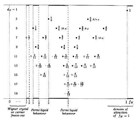
Figure 1: Observed Hall fractions $\sigma_{H}=n_{H}/d_{H}$ in the interval $0<\sigma_{H}\leq 1$.

If electromagnetic waves are sent through an “adiabatic hole” connecting two half-spaces one approximately finds an “integer quantization” of electromagnetic energy flux.

Our task is to attempt to provide a theoretical explanation of these remarkable experimental discoveries; hopefully one that enables us to predict further related effects.

Conductance quantization is observed in a rather wide temperature range. It appears that it is only found in systems without dissipative processes. When it is observed it is insensitive to small changes in the parameters specifying the system and to details of sample preparation; i.e., it has universality properties. — It will turn out that the key feature of systems exhibiting conductance quantization is that they have conserved chiral charges; (such conservation laws will only hold approximately, i.e., in slightly idealized systems). Once one has understood this point, the right formulae follow almost automatically, and one arrives at natural generalizations.

In order to give a first indication how the effects described here might be related to the two-dimensional chiral anomaly, we consider Example 1, the quantum Hall effect, in more detail. For readers not familiar with this remarkable effect [14], we summarize some of its key features.

A quantum Hall fluid (QHF) is an interacting electron gas confined to some domain in a two-dimensional plane (an interface between a semiconductor and an insulator, with compensating background charge) subject to a constant magnetic field $\vec{B}^{(0)}$ transversal to the confinement plane. Among experimental control parameters is the filling factor, $\nu$, defined by

$$\nu\;=\;\frac{n^{(0)}}{B^{(0)}\big{/}\left(\frac{h\,c}{e}\right)}$$

where $n^{(0)}$ is the (constant) electron density, $B^{(0)}$ is the component of the magnetic field $\vec{B}^{(0)}$ perpendicular to the plane of the fluid, and $\frac{h\,c}{e}$ is the quantum of magnetic flux. The filling factor $\nu$ is dimensionless.

Transport properties of a QHF in an external electric field (of small frequency) are described by the equation

$$\underline{J}\left(t,\underline{x}\right)\;=\;{~{}\sigma_{L}~{}~{}~{}\sigma_{H}\choose-\sigma_{H}~{}~{}\sigma_{L}}~{}~{}\underline{E}\left(t,\underline{x}\right)~{},$$ (2.4)

where $\underline{x}$ is a point in the sample, $\underline{J}$ is the bulk electric current parallel to the sample plane and $\underline{E}$ is the component of the external electric field parallel to the sample plane. Furthermore, $\sigma_{L}$ denotes the longitudinal conductivity, and $\sigma_{H}$ is the transverse – or Hall conductivity. In two dimensions, conductances and conductivities have the same dimension of [(charge)²/action], and it is not difficult to see that

$$G_{H}\;=\;\sigma_{H}~{}.$$ (2.5)

Experimentally, one observes that the longitudinal conductivity, $\sigma_{L}$, vanishes when the filling factor $\nu$ belongs to certain small intervals [9], a sign that there are no dissipative processes in the fluid. Such a QHF is called “incompressible”, for reasons explained below. Furthermore, on every interval of $\nu$ where $\sigma_{L}$ vanishes, the Hall conductivity $\sigma_{H}$ is a rational multiple of $\frac{e^{2}}{h}$ , as claimed in (2.2).

Next, we recall the basic equations of the electrodynamics of an incompressible QHF; see [8]. It is useful to combine the two-dimensional space of the fluid and time to a three-dimensional space-time. The electromagnetic field tensor of the system is given by

$$F_{\mu\nu}\;=\;\ \left(\begin{array}[]{lll}~{}~{}0&E_{1}&E_{2}\\ -E_{1}{}{}&~{}0&B\\ -E_{2}&-B{}{}&0\end{array}\right)~{},$$ (2.6)

where $E_{1}$ and $E_{2}$ are the components of an external electric field in the plane of the sample, and $B$ is the component of an external magnetic field, $\vec{B}$, perturbing the constant field $\vec{B}^{(0)}$ perpendicular to the sample plane; $\left(\vec{B}_{\rm total}=\vec{B}^{(0)}+\vec{B}\right)$.

We define $J^{0}(x)$ to denote the sum of the electron charge density in the space-time point $x=(t,\underline{x})$ and the uniform background charge density $en^{(0)}$. We set $J^{\mu}=(J^{0},\underline{J})$.

From the three-dimensional homogeneous Maxwell equations (Faraday’s law),

$$\partial_{\mu}\,F_{\nu\lambda}\;+\;\partial_{\nu}\,F_{\lambda\mu}\;+\;\partial_{\lambda}\,F_{\mu\nu}\;=\;0~{},$$ (2.7)

the continuity equation for the electric current density (conservation of electric charge),

$$\partial_{\mu}\,J^{\mu}\;=\;0~{},$$ (2.8)

and from the transport equation (2.4) with $\sigma_{L}=0$, it follows [8] that

$$J^{0}\;=\;\sigma_{H}\,B~{}.$$ (2.9)

Equations (2.4), for $\sigma_{L}=0$, and (2.9) can be combined to the equation

$$J^{\mu}\;=\;\sigma_{H}\;\varepsilon^{\mu\nu\lambda}\;F_{\nu\lambda}$$ (2.10)

of Chern-Simons electrodynamics, [5]. Eqs. (2.10) describe the response of an incompressible QHF to an external electromagnetic field (perturbing the constant magnetic field $\vec{B}^{(0)}$).

Unfortunately, eqs. (2.10) are compatible with the continuity equation (2.8) for $J^{\mu}$ only if $\sigma_{H}$ is constant throughout space-time. But realistic samples have a finite extension.

The finite extension of the sample, confined to a space-time region $\Omega=D\times{\mathbb{R}}$, where $D$ is e.g. a disk or an annulus, is taken into account by setting the Hall conductivity $\sigma_{H}(\cdot)$ to zero outside $\Omega$, i.e.,

$$\sigma_{H}(\xi)\;=\;\sigma_{H}\;\chi_{\Omega}(\xi)~{},$$ (2.11)

for $\xi\in{\mathbb{R}}^{3}$, where $\sigma_{H}$ is the (constant) value of the Hall conductivity inside the sample, and $\chi_{\Omega}$ is the characteristic function of $\Omega$. Taking the divergence of eq. (2.10), we get that

$$\partial_{\mu}\;J^{\mu}\;=\;\sigma_{H}\;\varepsilon^{\mu\nu\lambda}\;\left(\partial_{\mu}\,\chi_{\Omega}\right)~{}F_{\nu\lambda}~{},$$ (2.12)

i.e., $\partial_{\mu}J^{\mu}$ fails to vanish on the boundary, $\partial D$, of the sample. However, conservation of electric charge is a fundamental law of nature for closed systems. Thus, there must be an electric current, $J_{\partial\Omega}$, localized on the boundary $\partial\Omega$ of the sample space-time such that the total electric current

$$J_{\rm total}^{\mu}\;=\;J^{\mu}+J_{\partial\Omega}^{\mu}$$ (2.13)

satisfies the continuity equation. The boundary current $J_{\partial\Omega}^{\mu}$ must be tangential to the boundary $\partial\Omega$ of the sample space-time. Hence it determines a current density, $I^{\alpha}$, on the (1+1)-dimensional space-time $\partial\Omega$, where the index $\alpha$ refers to a choice of coordinates on $\partial\Omega$. Eq. (2.12) and the continuity equation for $J_{\rm total}^{\mu}$ then imply that

$$\partial_{\alpha}\,I^{\alpha}\;=\;-\,\sigma_{H}\;\varepsilon^{\alpha\beta}\;F_{\alpha\beta}~{}.$$ (2.14)

This equation identifies $I^{\alpha}$ as an anomalous current. Thus, there must be chiral modes (left-movers or right-movers, depending on the orientation of $\Omega$ and the direction of the external magnetic field) propagating along the boundary. They carry the well known diamagnetic edge currents. If ${\mathcal{J}}_{\ell}^{\alpha}$ (or ${\mathcal{J}}_{r}^{\alpha}$) denotes the corresponding quantum-mechanical current operator then the edge current $I^{\alpha}$ is given by the quantum-mechanical expectation value, $\langle{\mathcal{J}}_{\ell/r}^{\alpha}\rangle_{A}$, of ${\mathcal{J}}_{\ell}^{\alpha}$ (or ${\mathcal{J}}_{r}$). The currents ${\mathcal{J}}_{\ell}^{\alpha}$ have the anomalous commutators

$$\left[{\mathcal{J}}_{\ell}^{0}\left(t,\underline{x}\right),~{}{\mathcal{J}}_{\ell}^{0}\left(t,\underline{y}\right)\right]\;=\;\frac{i\,\sigma_{H}}{2\pi}\;\delta^{\prime}\left(\underline{x}-\underline{y}\right)~{},$$ (2.15)

see eqs. (1.21) and (1.16), and hence generate a chiral $\hat{u}(1)$-current algebra with central charge given by $\sigma_{H}$.

We now return to the physics of the bulk of an incompressible QHF. The absence of dissipation $(\sigma_{L}=0)$ in the transport of electric charge through the bulk can be explained by the existence of a mobility gap in the energy spectrum between the ground state energy of the QHF and the energies of extended, excited bulk states. This property motivates the term “incompressible”: It is not possible to add an additional electron to, or subtract one from the fluid by injecting only an arbitrarily small amount of energy. An important consequence of incompressibility is that the total electric charge is a good quantum number to label different sectors of physical states of an incompressible QHF (at zero temperature).

We propose to study the bulk physics of incompressible QHF’s in the scaling limit, in order to describe the universal transport laws of such fluids. For this purpose, we consider a QHF confined to a sample of diameter $\propto\theta$, where $\theta$ is a dimensionless scale factor. The scaling limit is the limit where $\theta\to\infty$, with distances and time rescaled by a factor $\theta^{-1}$. In rescaled coordinates, the fluid is thus confined to a sample of constant finite diameter.

The presence of a positive mobility gap in the system implies that, in the scaling limit, the effective theory describing an incompressible QHF must be a “topological field theory”. The states of a topological field theory are indexed by static, pointlike sources localized in the bulk and labelled by certain charge quantum numbers which generate a fusion ring; see [8, 11].

It is not difficult [10] to find the effective action, $S_{\rm eff}(A)$, in the scaling limit, where $A$ is the electromagnetic vector potential of the external electromagnetic field $F_{\mu\nu}$, see eq. (2.6). A possible starting point is eq. (2.10), relating the expectation value of the electric current to the external electromagnetic field:

$$J^{\mu}(\xi)\;=\;\delta\,S_{\rm eff}(A)\big{/}\delta\,A_{\mu}(\xi)\;=\;\sigma_{H}\;\varepsilon^{\mu\nu\lambda}\;F_{\nu\lambda}(\xi)~{}.$$ (2.16)

The solution of eq. (2.16) is

$$S_{\rm eff}(A)\;=\;\sigma_{H}\,S_{CS}(A)\;=\;\frac{\sigma_{H}}{2}\int_{\Omega}d^{3}\xi\;\varepsilon^{\mu\nu\lambda}\,A_{\mu}(\xi)\,\partial_{\nu}\,A_{\lambda}(\xi)~{},$$ (2.17)

i.e., $S_{\rm eff}$ is proportional to the Chern-Simons action $S_{CS}$. The Chern-Simons action is not invariant under gauge transformations of $A$ that do not vanish on the boundary $\partial\Omega$ of the sample. Since electromagnetic gauge invariance is a fundamental property of quantum-mechanical systems, eq. (2.17) for $S_{\rm eff}(A)$ must be corrected by a boundary term. Let $a$ denote the restriction of $A$ to the boundary $\partial\Omega$ of the sample. Then, as pointed out in eq. (1.71), the expression $W_{\ell/r}(a)\mp S_{CS}(A)$ is gauge-invariant, where $W_{\ell/r}(a)$ is the effective action of charged chiral modes propagating along $\partial\Omega$. Thus, in the scaling limit,

$$S_{\rm eff}(A)\;=\;\sigma_{H}\left[\mp W_{\ell/r}(a)+S_{CS}(A)\right]~{},$$ (2.18)

(depending on the sign of $\sigma_{H}$). It is well known that the action $W_{\ell/r}(a)$ is the generating function for the connected Green functions of the chiral current operators, ${\mathcal{J}}_{\ell/r}^{\alpha}$, on $\partial\Omega$, which generate a $\hat{u}(1)$-current algebra. Formula (2.18) plays an important rôle in understanding the physics of incompressible quantum Hall fluids.

In the next section, we consider systems of massless chiral modes in four-dimensional space-time, with physical properties some of which are related to the four-dimensional chiral anomaly, and which may play a significant rôle in the physics of the early universe.

3 Branes, axions and charged fermions

The very early universe is filled with a hot plasma of charged leptons, quarks, gluons, photons, … . At a time after the big bang when the temperature $T$ is of the order of 80 $TeV$ chirality flips of light charged leptons, in particular of right-handed electrons, constitute a dynamical process slower than the expansion rate of the universe. Thus, for $T\gtrsim$ 80 $TeV$, the chiral charges, $N_{\ell}$ and $N_{r}$, defined in eq. (1.50) of Sect. 1, are approximately conserved for electrons. They are related to an approximate chiral symmetry of the electronic sector of the standard model. Among other results, we shall attempt to show that if, in the very early universe, the chemical potentials of left-handed and right-handed electrons are different from each other, this may give rise to the generation of large, cosmic magnetic fields, [15]; (see also [7] for a similar, independent suggestion). This effect is, in a sense explained in Sects. 4 and 6, an effect in equilibrium statistical mechanics. However, this is precisely what may make it appear quite unnatural and implausible: The chiral charges, $N_{\ell}$ and $N_{r}$, are not really conserved; leptons are massive. The very early universe is not really in an equilibrium state, and the chemical potentials of left-handed and right-handed electrons neither have an unambiguous meaning, nor would they be space- and time-independent. It may then be wrong, or, at least, misleading, to invoke results from equilibrium statistical mechanics to explore effects in the physics of the very early universe.

A way out from these difficulties can be found by seeking inspiration from an analogy with the quantum Hall effect: Consider a quantum Hall fluid (QHF), confined to a strip of macroscopic width $\ell$ in the plane. If the QHF is incompressible then there are no light (gapless) modes propagating through the bulk of the sample; but, as shown in the last section, there are gapless, chiral modes propagating along the boundaries of the sample. Let $\Omega$ denote the space-time of the fluid; it is a slab of width $\ell$ in three-dimensional Minkowski space. The two components of the boundary, $\partial\Omega$, of $\Omega$ are denoted by $\partial_{+}\Omega$, $\partial_{-}\Omega$, respectively. As shown in the last section, eq. (2.18), (see also [10] for more details) the effective action of such an incompressible QHF (in the scaling limit) is given by

$$S_{\rm eff}(A)\;=\;\sigma_{H}\left[W_{\ell}\left(a_{+}\right)+W_{r}\left(a_{-}\right)-S_{CS}(A)\right]~{},$$ (3.1)

(if the direction of the external magnetic field $\vec{B}^{(0)}$ is chosen appropriately, given an orientation of $\Omega$). In (3.1), $A$ is an external electromagnetic vector potential on $\Omega$, and

$$a_{\pm}\;:=\;A\bigm{|}_{\partial_{\pm}\Omega}~{},$$ (3.2)

is the restriction of the 1-form $A$ to a component, $\partial_{\pm}\Omega$, of the boundary of $\Omega$; $W_{\ell/r}(\cdot)$ is the two-dimensional, anomalous effective action for charged, chiral (left-moving, or right-moving, respectively) surface modes propagating along $\partial_{+}\Omega,~{}\partial_{-}\Omega$, respectively; and $S_{CS}(\cdot)$ is the three-dimensional topological Chern-Simons action, see (2.17). Many universal features of the quantum Hall effect can be derived directly from eq. (3.1).

Suppose, in analogy to what we have just discussed, that the world, as known to us, is a movie showing the dynamics of light modes propagating along two parallel 3-branes in a five-dimensional space-time, $M$. More precisely, we imagine that $M$ is a slab of width $\ell$ in five-dimensional space-time, ${\mathbb{R}}^{5}$, the two components, $\partial_{+}M$ and $\partial_{-}M$, of the boundary of $M$ being identified with the two parallel 3-branes. Let us imagine that, through the five-dimensional bulk $M$ of the system, a massive, charged, four-component spinor field $\psi$ propagates. We consider the response of this system to coupling the charged fermions described by $\psi$ to a five-dimensional, external electromagnetic vector potential, $\hat{A}$. By $A_{\pm}$ we denote the four-dimensional vector potentials on $\partial_{\pm}M$ obtained by restricting $\hat{A}$ to $\partial_{\pm}M$. As discussed at the end of Sect. 1, there are chiral, left-handed or right-handed, charged, fermionic surface modes propagating along $\partial_{+}M$, $\partial_{-}M$, which are coupled to $A_{+},A_{-}$, respectively; see [6]. In eq. (1.74), the effective action of this system has been reported. It is given by

$${}S_{\rm eff}^{E}(\hat{A})\;=\;W_{\ell}(A_{+})+W_{r}(A_{-})-S_{CS}(\hat{A})$$

$${}~{}~{}~{}~{}~{}~{}~{}~{}~{}~{}~{}+(4\,\ell\,e^{2})^{-1}\int_{M}d^{5}\xi\;F_{\hat{A}}(\xi)^{2}+\ldots~{},$$ (3.3)

where the dots stand for terms $\sim O\left(\frac{1}{m}\right)$ , and the renormalization conditions have been chosen in such a way that the constant $e^{2}$ in front of the five-dimensional Maxwell term is the four-dimensional feinstructure constant. The components, $\hat{A}_{K}$, of $\hat{A}$ are denoted by

$$\hat{A}_{\mu}\;=:\;A_{\mu}~{},~{}~{}\mu\,=\,0,1,2,3,~{}~{}~{}\hat{A}_{4}\;=:\;\varphi~{},$$ (3.4)

i.e., $(\hat{A}_{K})=(A,\varphi),~{}K=0,1,2,3,4.$

In order to make contact with the laws of physics in four space-time dimensions, we should insist on the requirement that left-handed and right-handed fermions propagating along $\partial_{+}M$ and $\partial_{-}M$, respectively, couple to the same electromagnetic vector potential, i.e., that

$$A_{+}\left(x,x^{4}=\ell\right)\;=\;A_{-}\left(x,x^{4}=0\right)\;\equiv\;A(x)~{}.$$ (3.5)

This requirement is met if we assume that

$$\hat{A}\left(x,x^{4}\right)~{}~{}{\rm is~{}}independent~{}{\rm of~{}}x^{4}~{}.$$ (3.6)

In this case,

$$S_{CS}(\hat{A}) = \frac{i\,\ell}{32\,\pi^{2}}\int_{N}\varphi\left(F_{A}\wedge F_{A}\right)$$ (3.7)

$$= \frac{i\,\ell}{32\,\pi^{2}}\int_{N}d^{4}x\;\varphi(x)\;\varepsilon^{\mu\nu\lambda\rho}\,F_{\mu\nu}(x)\,F_{\lambda\rho}(x)$$

where $N\cong{\mathbb{R}}^{4}$ is a slice through $M$ parallel to $\partial_{\pm}M$, $\mu,\nu=0,1,2,3,$ and $F_{A}=(F_{\mu\nu})$ is the four-dimensional field tensor; (the trivial integration over $x^{4}$ has produced the factor $\ell$). Furthermore, the Maxwell term on the R.S. of (3.3) reduces to

$$\frac{1}{4\,e^{2}}~{}\left\{\int_{N}d^{4}x\,F_{\mu\nu}(x)\,F^{\mu\nu}(x)+\,2\int_{N}d^{4}x\,\left(\partial_{\mu}\varphi\right)(x)\left(\partial^{\mu}\varphi\right)(x)\right\}~{}.$$ (3.8)

Finally,

$$W_{\ell}\left(A_{+}=A\right)+W_{r}\left(A_{-}=A\right)\;=\;S_{\rm eff}^{E}(A)~{},$$ (3.9)

with $S_{\rm eff}^{E}(A)=S_{\rm eff}^{E}(A,Z=0)$ as in eqs. (1.29), (1.30). Thus, the complete effective action of the system is given by

$$S_{\rm eff}^{E}\left(\varphi;A\right) = S_{\rm eff}^{E}(A)~{}+~{}\frac{i\ell}{32\,\pi^{2}}\int_{N}\varphi\left(F_{A}\wedge F_{A}\right)$$ (3.10)

$$+ \frac{1}{4\,e^{2}}~{}\left\{\int_{N}d^{4}x\;F_{A}^{2}(x)+\,2\int_{N}d^{4}x\left(\nabla\varphi\right)^{2}(x)\right\}~{}.$$

Clearly, there is something quite unnatural about this approach: It is conditions (3.5) and (3.6)! If $A_{+}$ were different from $A_{-}$ then the fermionic effective action $S_{\rm eff}^{E}(A)=S_{\rm eff}^{E}(A,Z=0)$ would be replaced by $S_{\rm eff}^{E}(A,Z)$, where $A=\frac{1}{2}(A_{+}+A_{-})$ and $Z=\frac{1}{2}(-A_{+}+A_{-})$. Thus the surface modes would not only couple to the electromagnetic field, but also to a chiral gauge field $Z$ for which there is no experimental evidence, and the gauge fields would sample a five-dimensional space-time.

These unnatural features can be avoided by following Connes’ formulation of gauge theories with fermions [16]. Then the effective action displayed in eq. (3.10) can be reproduced as follows: One sets $M=N\times{\mathbb{Z}}_{2}$, $N\cong{\mathbb{R}}^{4}$ and treats the discrete “fifth dimension”, ${\mathbb{Z}}_{2}$, by using elementary tools from non-commutative geometry [16]. By adding a “non-commutative”, five-dimensional Chern-Simons action, as constructed in [17], to Connes’ version of the Yang-Mills action (for a U(1)-gauge field) and to the standard fermionic effective action, one can reproduce actions like the one in eq. (3.10); see [17]. There is no room, here, to review the details of these constructions.

In analogy to what we have discussed above, one may argue that string theories arise as effective theories of surface modes propagating along 9-branes in an “eleven-dimensional” space-time, starting from eleven-dimensional $M$-theory, (with anomalies of the surface theories cancelled by certain eleven-dimensional Chern-Simons actions). One realization of this idea appears in [18]. But we shall not pursue these ideas any further, in this review.

Instead, we ask whether the effective action in (3.10) ought to look familiar to people holding a conventional point of view that physical space-time is four-dimensional. The answer is “yes”! The scalar field $\varphi$ appearing in the effective action on the R.S. of (3.10) can be interpreted as the axion. The axion field was originally introduced by Peccei and Quinn [19] to solve the strong CP problem. There are various reasons, including, primarily, experimental ones, to feel unhappy about introducing an axion into the standard model. But there is also a good reason to do so: String theory predicts the existence of an axion, the “model-independent axion” first described by Witten [20].

The argument in favor of the model-independent axion goes as follows: String theory tells us that there must exist a second-rank antisymmetric tensor field, i.e., a two-form, $B_{\mu\nu}$. The gauge-invariant field strength, $H$, a three-form, corresponding to $B$ is given by

$$H\;=\;dB-\omega_{3YM}+\omega_{3G}~{},$$ (3.11)

where $d$ denotes exterior differentiation, and $\omega_{3YM}$ and $\omega_{3G}$ are the gauge-field (“Yang-Mills”) and gravitational (Lorentz) Chern-Simons three-forms. (The coefficients in front of these Chern-Simons forms are proportional to the number, $N_{f}$, of species of fermions coupled to the gauge- and gravitational fields. In the following we shall set $N_{f}=1$.) The field strength $H$ is invariant under the gauge transformations $B\to B+d\lambda$, where $\lambda$ is an arbitrary one-form, and under gauge- and local Lorentz transformations accompanied by shifts of $B$. The equation of motion of $H$ is

$$\partial^{\mu}\;H_{\mu\nu\lambda}\;=\;0~{},$$ (3.12)

or $\delta H=0$, where $\delta$ is the co-differential. We consider the components of $B_{\mu\nu}$ with $\mu,\nu=0,\ldots,3$ and assume that $B$ is independent of coordinates of internal dimensions (of the string theory target). Then, in four-dimensional (non-compact) space-time, the three-form $H$ is dual to a one-form, $Z$, and the equation of motion (3.12) becomes

$$\partial_{\mu}\,Z_{\nu}-\partial_{\nu}\,Z_{\mu}\;=\;0~{},~{}~{}{\rm or~{}}~{}d\,Z\;=\;0~{}.$$ (3.13)

By Poincaré’s lemma,

$$Z_{\mu}\;=\;\partial_{\mu}\;\alpha~{},~{}~{}{\rm or}~{}~{}Z\;=\;d\,\alpha~{},$$ (3.14)

where $\alpha$ is a scalar field. By (3.11), the scaling dimension of $\alpha$ is two. Introducing a constant, $\ell$, with the dimension of length, we set

$$\alpha\;=\;\frac{1}{\ell\,e^{2}}\ \varphi~{},$$ (3.15)

where $\varphi$ has scaling dimension = 1; ($e^{2}$ is the feinstructure constant).

From $d^{2}=0$ and (3.11) we obtain the equation

$$dH(x)\;=\;*{\mathcal{A}}(x)+{\rm const.}~{}{\rm tr}\,\left(R(x)\wedge R(x)\right)$$ (3.16)

where

$$*{\mathcal{A}}(x)\;=\;-~{}\frac{i}{32\,\pi^{2}}~{}\left(F(x)\wedge F(x)\right)$$ (3.17)

is the index density, see eq. (1.59), ($*$ denotes the Hodge dual), and $R(x)$ is the Riemann curvature tensor. Assuming that space-time is flat, hence $R=0$, and considering the special case, where the electromagnetic field is the only gauge field in the system, we obtain

$$dH\;=\;-~{}\frac{i}{32\,\pi^{2}}~{}\left(F_{A}\wedge F_{A}\right)~{}.$$ (3.18)

Recalling that

$$H\;=\;*~{}\left(\frac{1}{\ell\,e^{2}}~{}d\,\varphi\right)~{},$$

see (3.13)–(3.15), we find that (3.18) yields the following equation of motion for $\varphi$:

$$\square\;\varphi\;=\;-~{}\frac{i\ell\,e^{2}}{32\,\pi^{2}}~{}\ast\left(F_{A}\wedge F_{A}\right)~{}.$$ (3.19)

This equation is the Euler-Lagrange equation corresponding to the action functional

$$\frac{1}{2\,e^{2}}\int d^{4}x\,\left(\nabla\varphi\right)^{2}(x)+\frac{i\ell}{32\,\pi^{2}}\int\varphi\left(F_{A}\wedge F_{A}\right)~{},$$ (3.20)

which reproduces the R.S. of (3.10), up to the fermionic effective action and the Maxwell term! The second term in (3.20) can be understood as arising from coupling fermions to the axion. The term in the bare action of the fermions describing their coupling to the axion is given by

$$\frac{\ell^{2}}{2}\int d^{4}x\,H_{\mu\nu\lambda}\,\bar{\psi}\gamma^{\mu}\gamma^{\nu}\gamma^{\lambda}\psi\;=\;\frac{\ell}{2}\int d^{4}x\;\partial_{\mu}\varphi\bar{\psi}\gamma^{\mu}\gamma\psi~{},$$ (3.21)

where $\gamma=\gamma^{5}$. Carrying out the Berezin integral over the fermionic degrees of freedom — see eq. (1.29) — we find an effective action for the fermions given by

$$S_{\rm eff}^{E}\left(A,Z\;=\;\frac{\ell}{2}~{}d\varphi\right) = S_{\rm eff}^{E}\left(A,Z=0\right)\,-\,i\ell\int d^{4}x\;\varphi(x)\;{\mathcal{A}}(x)$$ (3.22)

$$= S_{\rm eff}^{E}(A)~{}-~{}\frac{i\ell}{32\,\pi^{2}}\int\varphi\left(F_{A}\wedge F_{A}\right)~{},$$

in accordance with (3.20). The first equation in (3.22) is eq. (1.41), the second follows from (1.59).

Thus, coupling charged Dirac fermions to an external electromagnetic vector potential $A$ and an axion $\varphi$ yields the effective action (3.22). Adding to it the Maxwell term and the kinetic energy term for $\varphi$, we again obtain the action (3.10)!

One may argue that, in any case, the presence of an axion in the theory may be an indication that there must exist extra (classical or, perhaps more plausibly, discrete or “non-commutative”) dimensions. But, for our applications in Sect. 6, this point is not important. What will matter is that the time derivative of the axion field will play the rôle of a, generally speaking, space-time dependent “chemical potential” for right-handed leptons.

But, quite independently of the properties of fermions (which, for example, may acquire masses through a Higgs-Kibble mechanism), the axion, $\varphi$, will turn out to be the driving force for a possible generation of large cosmic magnetic fields.

As our discussion at the beginning of this section, up to eq. (3.10), has shown it is legitimate to view a four-dimensional system of fermions in an external electromagnetic and an external axion field as the four-dimensional analogue of the edge degrees of freedom of an incompressible quantum Hall fluid. It supports electric currents analogous to the diamagnetic edge currents of a quantum Hall fluid.

4 Transport in thermal equilibrium through gapless
modes

In this section we prepare the ground for a theoretical explanation of effects such as the ones described in Sects. 2 (Examples 1 through 3) and 3. We consider a quantum-mechanical system ${\mathcal{S}}$ whose dynamics is determined by a Hamiltonian $H$, which is a selfadjoint operator on the Hilbert space ${\mathcal{H}}$ of pure state vectors of ${\mathcal{S}}$ with discrete energy spectrum. It is assumed that the system obeys conservation laws described by some conserved “charges” $N_{1},\ldots,N_{L}$ commuting with all observables of the system. Hence

$$\left[H,N_{\ell}\right]\;=\;0~{},~{}~{}\left[N_{\ell},N_{k}\right]\;=\;0~{},~{}~{}\ell,k\;=\;1,\ldots,L~{},$$ (4.1)

(e.g. in the sense that the spectral projections of $H$ and of $N_{\ell},N_{k}$ commute with one another, for all $k$ and $\ell$.) The system ${\mathcal{S}}$ is coupled to $L$ reservoirs, ${\mathcal{R}}_{1}\ldots,{\mathcal{R}}_{L}$, with the property that the expectation value of the conserved charge $N_{\ell}$ in a stationary state of ${\mathcal{S}}$ can be tuned to some fixed value through exchange of “quasi-particles” between ${\mathcal{S}}$ and ${\mathcal{R}}_{\ell}$, i.e., through a current between ${\mathcal{S}}$ and ${\mathcal{R}}_{\ell}$ that carries “$N_{\ell}$-charge”, for all $\ell=1,\ldots,L$ .

We are interested in describing a thermal equilibrium state of ${\mathcal{S}}$ coupled to ${\mathcal{R}}_{1},\ldots,{\mathcal{R}}_{L}$, at a temperature $T=(k_{B}\beta)^{-1}$. According to Gibbs, we should work in the grand-canonical ensemble. The reservoirs ${\mathcal{R}}_{1},\ldots{\mathcal{R}}_{L}$ then enter the description of the thermal equilibrium of ${\mathcal{S}}$ only through their chemical potentials $\mu_{1},\ldots,\mu_{L}$. The chemical potential $\mu_{\ell}$, is a thermodynamic parameter canonically conjugate to the charge $N_{\ell}$; in particular, the dimension of $\mu_{\ell}\cdot N_{\ell}$ is that of an energy. According to Landau and von Neumann, the thermal equilibrium state of ${\mathcal{S}}$ at temperature $(k_{B}\beta)^{-1}$ in the grand-canonical ensemble, with fixed values of $\mu_{1},\ldots,\mu_{L}$, is given by the density matrix

$$\rho_{\beta,\underline{\mu}}\;=\;\Xi_{\beta,\underline{\mu}}^{-1}~{}\exp\,\left[-\beta\,\left(H-\sum_{\ell=1}^{L}\mu_{\ell}\,N_{\ell}\,\right)\right]~{},$$ (4.2)

where the grand partition function $\Xi_{\beta,\underline{\mu}}$ is determined by the requirement that

$${\rm Tr}\;\rho_{\beta,\underline{\mu}}\;=\;1~{}.$$ (4.3)

(It is assumed here that ${\rm exp}\left[-\beta\left(H-\sum\mu_{\ell}N_{\ell}\right)\right]$  is a trace-class operator on ${\mathcal{H}}$, for all $\beta>0$; we are studying a system in a compact region of physical space.) The equilibrium expectation of a bounded operator, $a$, on ${\mathcal{H}}$ is defined by

$$\langle a\rangle_{\beta,\underline{\mu}}\;:=\;{\rm Tr}~{}\left(\rho_{\beta,\underline{\mu}}\,a\right)~{}.$$ (4.4)

Let ${\mathcal{J}}(x)=\left({\mathcal{J}}^{0}(x),\underline{{\mathcal{J}}}(x)\right)$ be a conserved quantum-mechanical current density of ${\mathcal{S}}$, where $x=(\underline{x},t)$, $t$ is time and $\underline{x}$ is a point of physical space contained inside ${\mathcal{S}}$. We are interested in calculating the expectation values of products of components of ${\mathcal{J}}$ in the state $\rho_{\beta,\underline{\mu}}$; in particular, we should like to calculate $\langle\underline{{\mathcal{J}}}(x)\rangle_{\beta,\underline{\mu}}$. Of course, if the dimension of space is larger than one, $\langle\underline{{\mathcal{J}}}(x)\rangle_{\beta,\underline{\mu}}$ vanishes unless rotation invariance is broken by some external field. If $\underline{{\mathcal{J}}}(x)$ is a vector current then $\langle\underline{{\mathcal{J}}}(x)\rangle_{\beta,\underline{\mu}}$ vanishes unless the state $\rho_{\beta,\underline{\mu}}$ is not invariant under space-reflection and time reversal. This happens if some of the charges $N_{1},\ldots,N_{L}$ are not invariant under space-reflection and time reversal, i.e., if they are chiral.

To say that ${\mathcal{J}}$ is conserved means that it satisfies the continuity equation

$$\partial_{\mu}\,{\mathcal{J}}^{\mu}\;=\;0~{},$$ (4.5)

where $x^{0}=t$ denotes time, and $\partial_{\mu}=\partial/\partial x^{\mu}$. If the space-time of the system ${\mathcal{S}}$ is topologically trivial (“star-shaped”) then eq. (4.5) implies that there is a globally defined vector field $\underline{\varphi}(x)$ such that

$${\mathcal{J}}^{0}(x)\;=\;\frac{q}{2\pi}\;{\rm div}\,\underline{\varphi}(x)~{},~{}~{}\underline{{\mathcal{J}}}(x)\;=\;-\,\frac{q}{2\pi}~{}\frac{\partial}{\partial t}~{}\underline{\varphi}(x)~{},$$ (4.6)

with $q$ the electric charge.

Let us suppose that $\underline{\varphi}(x)$ is an operator-valued distribution on ${\mathcal{H}}$, whose time-dependence is determined by the formal Heisenberg equation

$$\frac{\partial}{\partial t}\ \underline{\varphi}(x)\;=\;\frac{i}{\hbar}~{}\left[H,\underline{\varphi}(x)\right]~{}.$$ (4.7)

[Technically, we are treading on somewhat slippery ground here; but we shall proceed formally, in order to explain the key ideas on a few pages.] From (4.6) and (4.7) we derive that

$$\langle\underline{{\mathcal{J}}}(x)\rangle_{\beta,\underline{\mu}}\;=\;\frac{iq}{h}~{}\langle\left[H,\underline{\varphi}(x)\right]\rangle_{\beta,\underline{\mu}}~{}.$$ (4.8)

Formally, the R.S. of (4.8) vanishes, because $\langle(\cdot)\rangle_{\beta,\underline{\mu}}$ is a time-translation invariant state. However, the field $\underline{\varphi}$ turns out to have ill-defined zero-modes, and it is not legitimate to pretend that $[H,\underline{\varphi}(x)]=H\underline{\varphi}(x)-\underline{\varphi}(x)H$, because both terms on the R.S. are divergent, due to the zero-modes of $\underline{\varphi}$. What is legitimate is to claim that

$$\frac{\partial}{\partial t}~{}\underline{\varphi}(x)\;=\;\frac{i}{h}~{}\left[H-\sum_{\ell=1}^{L}\mu_{\ell}N_{\ell},\underline{\varphi}(x)\right]\;+\;\frac{i}{h}\sum_{\ell=1}^{L}\mu_{\ell}\left[N_{\ell},\underline{\varphi}(x)\right]~{},$$ (4.9)

and that the expectation value

$$\bigg{\langle}\left[H-\sum_{\ell=1}^{L}\mu_{\ell}N_{\ell},\underline{\varphi}(x)\right]\bigg{\rangle}_{\beta,\underline{\mu}}$$

vanishes. This can be seen by replacing the Hamiltonian $H$ by a regularized Hamiltonian $H^{(\varepsilon)}$ generating a dynamics that eliminates the zero-modes of $\underline{\varphi}$. One replaces the state $\rho_{\beta,\underline{\mu}}$ by a regularized state $\rho_{\beta,\underline{\mu}}^{(\varepsilon)}$ proportional to $\exp\left[-\beta\left(H^{(\varepsilon)}-\sum\mu_{\ell}N_{\ell}\right)\right]$, and we set

$$\langle a\rangle_{\beta,\underline{\mu}}^{(\varepsilon)}\;:=\;{\rm tr}\,\left(\rho_{\beta,\underline{\mu}}^{(\varepsilon)}a\right)~{},$$

for any bounded operator $a$ on ${\mathcal{H}}$. Then

$$\langle\underline{{\mathcal{J}}}(x)\rangle_{\beta,\underline{\mu}} = \lim_{\varepsilon\to 0}~{}\frac{iq}{h}~{}\bigg{\langle}\left[H^{(\varepsilon)}\;-\sum_{\ell=1}^{L}\mu_{\ell}N_{\ell},\underline{\varphi}(x)\right]\bigg{\rangle}_{\beta,\underline{\mu}}^{(\varepsilon)}$$ (4.10)

$$+ \lim_{\varepsilon\to 0}~{}\sum_{\ell=1}^{L}\frac{iq\mu_{\ell}}{h}~{}\langle\left[N_{\ell},\underline{\varphi}(x)\right]\rangle_{\beta,\underline{\mu}}^{(\varepsilon)}~{}.$$

Obviously

$$\bigg{\langle}\left[H^{(\varepsilon)}\;-\;\sum_{\ell=1}^{L}\mu_{\ell}N_{\ell},\underline{\varphi}(x)\right]\bigg{\rangle}_{\beta,\underline{\mu}}^{(\varepsilon)}\;=\;0~{},$$ (4.11)

and one might be tempted to expect that $\displaystyle\mathop{\lim}_{\varepsilon\to 0}\langle\left[N_{\ell},\underline{\varphi}(x)\right]\rangle_{\beta,\underline{\mu}}^{(\varepsilon)}$ vanishes, for all $\ell$, because the charges $N_{\ell}$ are conserved. However, as long as the regularization is present $(\varepsilon\neq 0)$, these charges are not conserved, and there is no guarantee that the second term on the R.S. of (4.10) vanishes!

We conclude that

$$\langle\underline{{\mathcal{J}}}(x)\rangle_{\beta,\underline{\mu}} = \lim_{\varepsilon\to 0}~{}\sum_{\ell=1}^{L}~{}\frac{iq\mu_{\ell}}{h}~{}\langle\left[N_{\ell},\underline{\varphi}(x)\right]\rangle_{\beta,\underline{\mu}}^{(\varepsilon)}$$ (4.12)

$$=: \sum_{\ell=1}^{L}~{}\frac{iq\mu_{\ell}}{h}~{}\langle\left[N_{\ell},\underline{\varphi}(x)\right]\rangle_{\beta,\underline{\mu}}~{}.$$

Eq. (4.12) might be called a current sum rule.

Let us assume that the conserved charges $N_{\ell},\ell=1,2,\ldots,$ are given as integrals of the 0-components of conserved currents over space. Then the current sum rule (4.12) implies that if $\langle\underline{{\mathcal{J}}}(x)\rangle_{\beta,\underline{\mu}}\neq 0$ there must be gapless modes in the system. The proof, see [7], is analogous to the proof of the Goldstone theorem in the theory of broken continuous symmetries.

The sum rule (4.12) is the main result of this section. A careful derivation of equation (4.12) and of our analogue of the Goldstone theorem could be given by using the operator-algebra approach to quantum statistical mechanics [21]. But, in order to reach our punch line on a reasonable number of pages, we refrain from entering into a careful technical discussion.

5 Conductance quantization in ballistic wires and in incompressible quantum Hall fluids

In this section, we combine the results of Sects. 2 and 4, in order to gain insight into the phenomena of conductance quantization, as discussed at the beginning of Sect. 2. We first study a ballistic wire, i.e., a very thin, long, clean conductor without back scattering centers (impurities). The ends of the wire are connected to two reservoirs filled with electrons at chemical potentials $\mu_{\ell},\mu_{r}$, respectively, with

$$\mu_{\ell}-\mu_{r}\;=\;V~{},$$ (5.1)

where $V$ is the voltage drop through the wire.

A ballistic wire is a three-dimensional, elongated metallic object with a tiny cross section in the plane perpendicular to its principal axis. Thus, at low temperature, the three-dimensional nature of the wire merely implies that there are several, say $N$, species of electrons labelled by discrete quantum numbers that originate from the motion in the plane perpendicular to the axis of the wire. Every species of electrons forms a one-dimensional Luttinger liquid [22], and these Luttinger liquids may interact with each other. Every Luttinger liquid has two conserved vector current operators, ${\mathcal{J}}^{(i,s)\mu}$, and conserved chiral current operators, $\widehat{{\mathcal{J}}}_{\ell/r}^{(i,s)\mu}$, where $s=\uparrow,\downarrow$ denotes the magnetic quantum number of the electrons in the i^th Luttinger liquid (“spin up” and “spin down”), and $i=1,\ldots,N$. The chiral current operators $\widehat{{\mathcal{J}}}_{\ell}^{(i,s)\mu}$ are as in eqs. (1.21)–(1.23). The total electric current operator and the total chiral current operators are given by

$${\mathcal{J}}^{\mu}\;=\;\sum_{i=1\atop s=\uparrow,\downarrow}^{N}{\mathcal{J}}^{(i,s)\mu}~{},~{}~{}\widehat{{\mathcal{J}}}_{\ell/r}^{\mu}\;=\;\sum_{i=1\atop s=\uparrow,\downarrow}^{N}\widehat{{\mathcal{J}}}_{\ell,r}^{(i,s)\mu}~{}.$$ (5.2)

They are conserved. The total electric charge operators counting the electric charges of chiral (left-moving and right-moving) modes in the wire are the operators $N_{\ell}$ and $N_{r}$ defined in eq. (1.24). Their expectation values in a thermal equilibrium state of the wire are tuned by the chemical potentials, $\mu_{\ell},\mu_{r}$, respectively, of the reservoirs at the right and left end of the wire.

Imagine that the wire is kept at a constant temperature $\beta^{-1}$. Our description of the electron gas in the wire in terms of a finite number of Luttinger liquids correctly captures electric transport properties of the wire only if $\beta^{-1}$ and $eV$, with $e$ the elementary electric charge, are tiny as compared to the energy scale of the motion in the plane perpendicular to the axis of the wire. (However, $\beta^{-1}$ and $eV$ should be large as compared to the energy scale of weak back scattering centers.) We shall assume that these conditions are met. Then we may apply the current sum rule (4.12) derived in the last section, and the formulae for the anomalous commutators derived in Sect. 1, see (1.16) and the equation after (1.24), in order to calculate the electric current, $I$, in the wire corresponding to a voltage drop $V$. The current sum rule (4.12) yields

$$I = \langle\underline{{\mathcal{J}}}(x)\rangle_{\beta,\underline{\mu}}$$ (5.3)

$$= \frac{iq}{h}~{}\left\{\mu_{\ell}\,\big{\langle}\left[N_{\ell},\underline{\varphi}(x)\right]\big{\rangle}_{\beta,\underline{\mu}}+\mu_{r}\,\big{\langle}\left[N_{r},\underline{\varphi}(x)\right]\big{\rangle}_{\beta,\underline{\mu}}\right\}~{},$$

where $\underline{\varphi}$ is the potential of the current ${\mathcal{J}}^{\mu}$. Since the currents ${\mathcal{J}}^{(i,s)\mu}$ of all the Luttinger liquids are conserved, every one of them can be derived from a potential, $\varphi^{(i,s)}$,

$${\mathcal{J}}^{(i,s)\mu}(x)\;=\;\frac{q}{2\pi}~{}\varepsilon^{\mu\nu}\left(\partial_{\nu}\,\varphi^{(i,s)}\right)(x)~{},$$ (5.4)

see eq. (1.11), and $q=-e$, because the electric charge of an electron is equal to minus the elementary electric charge.

Plugging (5.4) and (5.2) into eq. (5.3) and recalling eq. (1.24) and the anomalous commutator

$${}\left[\widehat{{\mathcal{J}}}_{\ell/r}^{(i,s)0}\left(\underline{y},t\right),~{}\varphi^{(i^{\prime},s^{\prime})}\left(\underline{x},t\right)\right]$$

$$~{}~{}~{}~{}~{}=~{}\pm i~{}\frac{e}{2\pi}~{}\delta_{ii^{\prime}}\,\delta_{ss^{\prime}}\,\delta\left(\underline{x}-\underline{y}\right)~{},$$ (5.5)

see eqs. (1.11), (1.15), (1.16), we find that

$$I = -~{}\frac{ie}{h}~{}\sum_{i=1\atop s=\uparrow,\downarrow}^{N}\left\{\mu_{\ell}\bigg{\langle}\left[N_{\ell}^{(i,s)},~{}\varphi^{(i,s)}\left(\underline{x},t\right)\right]\bigg{\rangle}_{\beta,\underline{\mu}}\right.$$ (5.6)

$${}~{}~{}~{}~{}~{}~{}~{}~{}~{}~{}~{}~{}~{}~{}~{}~{}~{}~{}\left.+~{}\mu_{r}\,\bigg{\langle}\left[N_{r}^{(i,s)},~{}\varphi^{(i,s)}\,\left(\underline{x},t\right)\right]\bigg{\rangle}_{\beta,\underline{\mu}}\right\}$$

$$= \frac{e^{2}}{h}\times 2N\times\left(\mu_{\ell}-\mu_{r}\right)$$

$$= 2N~{}\frac{e^{2}}{h}~{}V~{}.$$

Thus, we have derived the formula

$$G_{W}\;=\;\frac{I}{V}\;=\;2N~{}\frac{e^{2}}{h}~{},$$ (5.7)

as claimed in Example 2 at the beginning of Sect. 2.

Of course, the number, $N$, of Luttinger liquids of electrons in the wire depends on the mean Fermi energy of the wire (at zero temperature) and hence on the electron density in the wire and can be tuned.

The quantization of the Hall conductance of an incompressible Hall fluid in a Hall sample with e.g. an annular (Corbino) geometry (see Example 1) can be understood by using very similar arguments as in the example of quantum wires. Let $V$ denote the voltage drop between the outer and the inner edge of the sample. We assume that $eV$ and the temperature $\beta^{-1}$ are tiny, as compared to the mobility gap in the bulk of the fluid. Let us also assume, temporarily, that the electric field created by connecting the outer and inner edge to the two leads of a battery with voltage drop $V$ does not penetrate into the bulk of the sample (i.e., that, in the bulk, it is screened completely). If this assumption (which will actually turn out to be irrelevant, later) is made then the entire Hall current, $I_{H}$, in the sample is carried by the chiral modes propagating along the edges of the sample, i.e., $I_{H}$ is given by the expectation value of the sum, $\widehat{{\mathcal{J}}}_{\ell}^{1}+\widehat{{\mathcal{J}}}_{r}^{1}$, of the edge currents, $\widehat{{\mathcal{J}}}_{\ell}^{\mu},\widehat{{\mathcal{J}}}_{r}^{\mu}$. For an appropriate choice of orientation, $\widehat{{\mathcal{J}}}_{\ell}^{\mu}$ is the current at the outer edge and $\widehat{{\mathcal{J}}}_{r}^{\mu}$ is the current at the inner edge of the sample. The two edges are separated by the bulk, and, for a macroscopic sample, tunnelling of quasi-particles from one edge to the other one can be neglected for all practical purposes. This implies that the currents, $\widehat{{\mathcal{J}}}_{\ell}^{\mu}$ and $\widehat{{\mathcal{J}}}_{r}^{\mu}$, and hence the charge operators $N_{\ell}$ and $N_{r}$ defined in eq. (1.24), are conserved to very high accuracy. The anomalous commutators of $\widehat{{\mathcal{J}}}_{\ell}^{\mu}$ and $\widehat{{\mathcal{J}}}_{r}^{\mu}$ are given in eq. (2.15), and the analogue of Eqs. (1.11) and (5.4) is

$${\mathcal{J}}^{\mu}(x)\;=\;e~{}\frac{\sqrt{f_{H}}}{2\pi}~{}\varepsilon^{\mu\nu}~{}\left(\partial_{\nu}\varphi\right)(x)~{}.$$ (5.8)

Inserting these equations into the current sum rule (4.12), one finds that

$$I_{H} = -\;\frac{e}{h}~{}\sqrt{f_{H}}~{}\left\{\mu_{\ell}\big{\langle}\left[N_{\ell},\varphi\left(\underline{x},t\right)\right]\big{\rangle}_{\beta,\underline{\mu}}+\mu_{r}\big{\langle}\left[N_{r},\varphi\left(\underline{x},t\right)\right]\big{\rangle}_{\beta,\underline{\mu}}\right\}$$ (5.9)

$$= \frac{e^{2}}{h}~{}f_{H}\,\left(\mu_{\ell}-\mu_{r}\right)$$

$$= \sigma_{H}~{}V~{}.$$

These arguments do not make it clear why the Hall fraction $f_{H}=\left(e^{2}/h\right)^{-1}\sigma_{H}$ is a rational number, and we have no clue, so far, which rational numbers may turn up in physical samples. Understanding the rational quantization of $f_{H}$ is not quite an easy matter; see [8, 11]. Here we can only sketch some key ideas. Let $\psi(\underline{x},t)$ denote the field (a “chiral vertex operator”) creating an electron or a hole propagating along the inner (or along the outer) edge of the sample. This field has the form

$$\psi\left(\underline{x},t\right)\;=\;:\,e^{iq\varphi_{\ell/r}(\underline{x},t)}\;:\;\varepsilon\left(\underline{x},t\right)~{},$$ (5.10)

where $q$ is a real number to be determined, $\varphi_{\ell/r}(\underline{x},t)$ is the potential of the conserved chiral edge current, i.e., it is a massless, chiral free field, and $\varepsilon(\underline{x},t)$ is an electrically neutral so-called simple current of a rational chiral conformal field theory describing chiral modes of zero charge propagating along the edge. The field $\psi(\underline{x},t)$ must carry electric charge $\pm e$. Using formula (5.8) and recalling that $\varepsilon$ has zero electric charge, we find that

$$q\;=\;1\big{/}\sqrt{f_{H}}~{}.$$ (5.11)

Furthermore, the field $\psi(\underline{x},t)$ must obey Fermi statistics (because electrons and holes are fermions). Hence it must have half-integer “conformal spin”, i.e.,

$$s_{\psi}\;\equiv\;1/2~{}{\rm mod.~{}}1~{}.$$ (5.12)

By eq. (5.10), the conformal spin of $\psi$ is given by

$$s_{\psi}\;=\;\frac{q^{2}}{2}~{}+~{}s_{\varepsilon}\;=\;\frac{1}{2\,f_{H}}~{}+~{}s_{\varepsilon}~{},$$ (5.13)

where $s_{\varepsilon}$ is the conformal spin of $\varepsilon$. Because $\varepsilon$ is a simple current of a rational chiral conformal field theory, $s_{\varepsilon}$ is a rational number, i.e., $s_{\varepsilon}=\frac{k}{\ell}$, with $k$ and $\ell$ two relatively prime integers. Thus (5.12) and (5.13) imply that

$$\frac{1}{2\,f_{H}}~{}+~{}\frac{k}{\ell}~{}\equiv~{}1/2~{}{\rm mod.~{}}1~{}.$$ (5.14)

It follows that $f_{H}$ is a rational number. For more details see [8, 23, 24] and, especially, [11]. Properties of the rational chiral conformal field theories that may appear in the context of the quantum Hall effect are discussed in [8, 11]. One noteworthy result is that, unless $f_{H}$ is an integer, there must be chiral modes (quasi-particles) of fractional electric charge and fractional statistics, sometimes called Laughlin vortices, propagating along the edges of the sample.

Let us see what happens if the electric field $\underline{E}$ can penetrate into the bulk of an incompressible quantum Hall fluid. Electric transport in such Hall fluids can be understood by combining the arguments outlined above with Hall’s law in the bulk. The total Hall current, $I_{H}$, is given by

$$I_{H}\;=\;I_{H}^{\rm edge}+I_{H}^{\rm bulk}~{},$$ (5.15)

where $I_{H}^{\rm edge}$ is the edge current studied above, and $I_{H}^{\rm bulk}$ is a current carried by extended bulk states. Let $\gamma$ denote an arbitrary smooth oriented curve connecting a point on the inner edge to a point on the outer edge of the sample. Then

$$I_{H}^{\rm bulk}\;=\;-\sum_{k,\ell}\int_{\gamma}J^{k}\left(\underline{x},t\right)\;\varepsilon_{k\ell}\;ds^{\ell}\left(\underline{x}\right)~{},$$ (5.16)

where $J^{k}$ is the $k$-component of the bulk current; see eq. (2.4). As usual,

$$J^{k}\left(\underline{x},t\right)\;=\;\big{\langle}{\mathcal{J}}^{k}\left(\underline{x},t\right)\big{\rangle}_{A}\;=\;\delta\,S_{\rm eff}(A)\big{/}\delta\,A_{k}\left(\underline{x},t\right)~{}.$$ (5.17)

By eqs. (2.17), (2.18), the R.S. of (5.17) is given by

$$\delta\,S_{\rm eff}(A)\big{/}\delta\,A_{k}\left(\underline{x},t\right)\;=\;\sigma_{H}\;\varepsilon_{k\ell}\;E^{\ell}\left(\underline{x},t\right)~{},$$ (5.18)

see also (2.4) (with $\sigma_{L}=0$). Thus

$$I_{H}^{\rm bulk}\;=\;\sigma_{H}\int_{\gamma}\underline{E}\left(\underline{x},t\right)\,\cdot\,d\underline{s}(\underline{x})~{}.$$ (5.19)

We have shown in eq. (5.9) that

$$I_{H}^{\rm edge}\;=\;\sigma_{H}\,\left(\mu_{\ell}-\mu_{r}\right)~{}.$$ (5.20)

Thus, combining (5.15), (5.19) and (5.20), we conclude that

$$I_{H}\;=\;I_{H}^{\rm edge}+I_{H}^{\rm bulk}\;=\;\sigma_{H}\,\left(\mu_{\ell}-\mu_{r}+\int_{\gamma}\underline{E}\left(\underline{x},t\right)\,\cdot\,d\underline{s}\left(\underline{x}\right)\right)~{}.$$ (5.21)

But the expression in the parenthesis on the R.S. of (5.21) is nothing but the total voltage drop $V$ between the outer and the inner edge. Hence (5.21) implies that

$$I_{H}\;=\;\sigma_{H}\;V~{},$$ (5.22)

as desired.

Transport phenomena such as heat conduction through a quantum wire or a Hall sample (see Example 3 at the beginning of Sect. 2) can be studied along similar lines: In a physical system where modes of different chirality do not interact with each other (such as the modes at the inner and at the outer edge of the sample containing an incompressible Quantum Hall fluid) the left-moving and the right moving modes can be coupled to different reservoirs at different temperatures $\beta_{\ell}^{-1}$ and $\beta_{r}^{-1}$. This results in a non-zero heat current given by an expectation value of the component $T^{01}$ of the energy-momentum tensor of the conformal field theory describing the chiral modes in an equilibrium state where the left-movers are at temperature $\beta_{\ell}^{-1}$ and the right-movers at temperature $\beta_{r}^{-1}\neq\beta_{\ell}^{-1}$. (Such expectation values can be calculated from Virasoro characters.) These ideas lead to a conceptually clean understanding of the effects described in Example 3 at the beginning of Sect. 2.

6 A four-dimensional analogue of the Hall effect, and the generation of large, cosmic magnetic fields in the early universe

In this section, we further explore the four-dimensional analogue of the Hall effect described in Sect. 3. We shall apply our findings to exhibit effects that may play an important rôle in early-universe cosmology. Our results represent an elaboration upon those in [15, 7].

We start our analysis by studying a system of massless Dirac fermions coupled to an external electromagnetic field in four-dimensional Minkowski space. Using results derived in Sects. 1 and 4, we derive equations analogous to eqs. (5.3)–(5.6) for the conductance of a quantum wire.

From Sect. 1 we recall the expression for the anomalous commutators between vector- and axial-vector — or chiral currents.

$$\left[\widehat{{\mathcal{J}}}_{\ell/r}^{0}\left(t,\underline{x}\right),~{}\widehat{{\mathcal{J}}}_{\ell/r}^{0}\left(t,\underline{y}\right)\right]\;=\;\pm~{}i~{}\frac{q^{2}}{4\pi^{2}}~{}\left(\underline{B}\left(\underline{x},t\right)\,\cdot\,\underline{\nabla}\right)\;\delta\left(\underline{x}-\underline{y}\right)~{},$$ (6.1)

where $q$ is the charge of the fermions — see eq. (1.62) — and

$$\left[\widehat{{\mathcal{J}}}_{\ell}^{0}\left(t,\underline{x}\right)\,,~{}\widehat{{\mathcal{J}}}_{r}^{0}\left(t,\underline{y}\right)\right]\;=\;0~{}.$$ (6.2)

With (1.45) and (1.48), these equations yield

$$\left[\widehat{{\mathcal{J}}}_{\ell/r}^{0}\left(t,\underline{y}\right)\,,~{}{\mathcal{J}}^{0}\left(t,\underline{x}\right)\right]\;=\;\pm~{}i~{}\frac{q^{2}}{8\pi^{2}}~{}\left(\underline{B}\left(\underline{y},t\right)\,\cdot\,\underline{\nabla}_{\underline{x}}\right)~{}\delta\left(\underline{x}-\underline{y}\right)~{},$$ (6.3)

where ${\mathcal{J}}^{\mu}$ is the $\mu$-component of the conserved vector current. In Sect. 4, we have introduced the vector potential, $\underline{\varphi}$, of ${\mathcal{J}}^{\mu}$:

$${\mathcal{J}}^{0}(x)\;=\;\frac{q}{2\pi}~{}{\rm div}\;\underline{\varphi}(x)\,,~{}\underline{{\mathcal{J}}}(x)\;=\;-\,\frac{q}{2\pi}~{}\frac{\partial}{\partial t}~{}\underline{\varphi}(x)~{}.$$ (6.4)

Eqs. (6.3) and (6.4) imply that

$$\left[\widehat{{\mathcal{J}}}_{\ell/r}^{0}\left(\underline{y},t\right)\,,~{}\underline{\varphi}\left(\underline{x},t\right)\right] = \pm~{}i~{}\frac{q}{4\pi}~{}\underline{B}\left(\underline{y},t\right)~{}\delta\left(\underline{x}-\underline{y}\right)$$ (6.5)

$$\pm {\rm curl~{}}\underline{\Pi}\left(\underline{x}-\underline{y},t\right)$$

where $\underline{\Pi}$ is some vector-valued distribution.

Next, we recall that the operators

$$N_{\ell/r}\;:=\;\int d\underline{y}~{}\widehat{{\mathcal{J}}}_{\ell/r}^{0}\;\left(\underline{y},t\right)$$ (6.6)

are conserved. They are interpreted as the electric charge operators for left-handed/right-handed fermionic modes. The chemical potentials conjugate to $N_{\ell/r}$ are denoted by $\mu_{\ell/r}$. Let us imagine that, at very early times in the evolution of our universe (or others), there was an asymmetry in the population of left-handed and right-handed fermionic modes, (as argued in [15] for the example of electrons before the electroweak phase transition). Then

$$\mu_{\ell}~{}\neq~{}\mu_{r}~{},$$ (6.7)

in the state of the universe at those very early times. Let us furthermore imagine that the state of the universe at those early times was, to a good approximation, a thermal equilibrium state at an inverse temperature $\beta$ ( $\lesssim\left(80~{}TeV\right)^{-1}$, as argued in [15]) and with chemical potentials $\mu_{\ell}$ and $\mu_{r}$. (It may well be that this is an unrealistic assumption. — It will subsequently turn out that it is unimportant!)

Under these assumptions, we may apply the current sum rule (4.12) derived in Sect. 4. Combining eqs. (6.5), (6.6) and (4.12), and using that $\int\limits_{{\mathbb{R}}^{3}}d\underline{y}~{}{\rm curl~{}}\underline{\Pi}\left(\underline{x}-\underline{y},t\right)=0$, for all $\underline{x},t$, we find that

$$\big{\langle}\underline{{\mathcal{J}}}(x)\big{\rangle}_{\beta,\underline{\mu}} = \frac{iq}{h}~{}\left\{\mu_{\ell}\big{\langle}\left[N_{\ell},\underline{\varphi}(x)\right]\big{\rangle}_{\beta,\underline{\mu}}\;+\;\mu_{r}\;\big{\langle}\left[N_{r},\underline{\varphi}(x)\right]\big{\rangle}_{\beta,\underline{\mu}}\right\}$$ (6.8)

$$= -~{}\frac{q^{2}}{4\pi\,h}~{}\left(\mu_{\ell}-\mu_{r}\right)~{}\underline{B}(x)~{},$$

as claimed in [7]. This equation is the analogue of (5.6).

Treating the electromagnetic field as a classical, but dynamical field, its dynamics is governed by Maxwell’s equations,

$$\underline{\nabla}\,\cdot\,\underline{B}\;=\;0~{},~{}~{}\underline{\nabla}\wedge\underline{E}\;+\;\partial_{t}\,\underline{B}\;=\;0~{},$$

and

$$\underline{\nabla}\,\cdot\,\underline{E}\;=\;\langle{\mathcal{J}}^{0}\rangle_{\beta,\underline{\mu}}~{},~{}~{}\underline{\nabla}\wedge\underline{B}-\partial_{t}\,\underline{E}\;=\;\langle\underline{{\mathcal{J}}}\rangle_{\beta,\underline{\mu}}~{}.$$ (6.9)

There is no reason to imagine that the charge density, $\langle{\mathcal{J}}^{0}\rangle_{\beta,\underline{\mu}}$, in the very early universe is different from zero. In the last equation of (6.9), the current on the R.S. is given by eq. (6.8). Actually, assuming that there are some dissipative processes evolving in the early universe, an equation for the current,

$$\underline{J}(x)\;:=\;\langle\underline{{\mathcal{J}}}(x)\rangle_{\beta,\underline{\mu}}~{},$$

more realistic than (6.8) may be

$$\underline{J}(x)\;=\;\sigma_{L}\,\underline{E}\,(x)\;+\;\sigma_{T}\,V\,\underline{B}\,(x)~{},$$ (6.10)

where $\sigma_{L}$ is an Ohmic longitudinal conductivity, and

$$\sigma_{T}\;:=\;-~{}\frac{q^{2}}{4\pi\,h}$$ (6.11)

is the analogue of the “transverse” or Hall conductivity; furthermore,

$$V\;:=\;\mu_{\ell}-\mu_{r}$$ (6.12)

is the analogue of the voltage drop considered in the Hall effect. The quantity $\sigma_{T}$ is “quantized”, just like the Hall conductivity: If there are $N>1$ species of charged, massless fermions, with electric charges $q_{1},\ldots,q_{N},$ then

$$\sigma_{T}\;=\;-~{}\frac{1}{4\pi\,h}~{}\left(\sum_{j=1}^{N}q_{j}^{2}\right)~{},$$ (6.13)

which is the precise analogue of a formula for the quantization of the Hall conductivity derived in [8], and, for $q_{j}=\pm\,e,~{}j=1,\ldots,N,$ of eq. (5.6).

Let us temporarily assume that $\sigma_{L}=0$, (i.e., we neglect dissipative processes). Then Maxwell’s equations, together with eq. (6.10) (for $\sigma_{L}=0$) and the assumption that the charge density vanishes, yield the following system of linear equations:

$${}\underline{\nabla}\,\cdot\,\underline{B}\;=\;0~{},~{}~{}\underline{\nabla}\wedge\underline{E}\;+\;\partial_{t}\,\underline{B}\;=\;0~{},$$

$${}\underline{\nabla}\,\cdot\,\underline{E}\;=\;0~{},~{}~{}\underline{\nabla}\wedge\underline{B}\,-\,\partial_{t}\,\underline{E}\;=\;\sigma_{T}\,V\,\underline{B}~{}.$$ (6.14)

Because all coefficients are constant, these equations can be solved by Fourier transformation, and it is enough to construct propagating wave solutions corresponding to an arbitrary, but fixed wave vector $\underline{k}$. The equations $\underline{\nabla}\cdot\underline{B}=\underline{\nabla}\cdot\underline{E}=0$ imply that

$$\underline{k}\,\cdot\,\widehat{\underline{B}}\;=\;\underline{k}\,\cdot\,\widehat{\underline{E}}\;=\;0~{},$$ (6.15)

i.e., that only the components of the Fourier transforms $\widehat{\underline{B}}$ and $\widehat{\underline{E}}$ of $\underline{B}$ and $\underline{E}$ (evaluated at the wave vector $\underline{k}$) perpendicular to $\underline{k}$ can be non-zero. Denoting the components of $\widehat{\underline{B}}$ and $\widehat{\underline{E}}$ perpendicular to $\underline{k}$ by $\widehat{\underline{B}}^{T},~{}\widehat{\underline{E}}^{T}$, respectively, the remaining equations in (6.14) yield

$$\partial_{t}~{}{~{}\widehat{\underline{E}}^{T}\choose~{}\widehat{\underline{B}}^{T}~{}}~{}=~{}K(\underline{k})~{}{~{}\widehat{\underline{E}}^{T}\choose~{}\widehat{\underline{B}}^{T}~{}}~{},$$ (6.16)

where (in an orthonormal basis chosen in the plane perpendicular to $\underline{k}$) the matrix $K(\underline{k})$ is given by

$$K\,(\underline{k})\;=\;\left(\begin{array}[]{cccc}~{}0{}&~{}0{}&~{}-\,\sigma_{T}\,V{}&~{}-\,i\,k{}\\ ~{}0{}&~{}0{}&i\,k{}&~{}-\,\sigma_{T}\,V{}\\ ~{}0{}&~{}i\,k{}&~{}0{}&~{}0{}\\ ~{}-\,i\,k{}&~{}0{}&~{}0{}&~{}0{}\end{array}\right)$$ (6.17)

with $k=|\underline{k}|$. The circular frequency of a propagating wave solution of (6.14) with wave vector $\underline{k}$ is given by $\omega(\underline{k})$, where $i\,\omega(\underline{k})$ is an eigenvalue of $K(\underline{k})$. By (6.17),

$$\omega\,(\underline{k})^{2}\;=\;k^{2}~{}\pm~{}k\,\sigma_{T}\,V~{},$$ (6.18)

as one readily checks. Thus, if

$$|\underline{k}|\;=\;k\,<\,\sigma_{T}\,V$$ (6.19)

there are two purely imaginary frequencies, and eqs. (6.14) have solutions $\left(\underline{B}\left(\underline{x},t\right),~{}\underline{E}\left(\underline{x},t\right)\right)$ growing exponentially fast in time and with the property that

$$\underline{B}\left(\underline{x},t\right)\,\cdot\,\underline{E}\left(\underline{x},t\right)\;\neq\;0~{}.$$ (6.20)

It is almost as easy to solve Maxwell’s equations (6.9), with $\underline{J}$ given by (6.10), for $\sigma_{L}\neq 0$. For wave vectors $\underline{k}$ satisfying

$$\sigma_{L}^{2}\;<\;|\underline{k}|\;\sigma_{T}\,V\;<\;\left(\sigma_{T}\,V\right)^{2}~{},$$ (6.21)

one again finds exponentially growing electromagnetic fields; (perturbation theory). Dissipative processes will subsequently damp out electric fields.

In [15], calculations similar to those just presented are used to argue that, in the very early universe, large, cosmic electromagnetic fields may have been generated as a consequence of an asymmetric population of left-handed and right-handed electron modes $(q=-e)$. However, these arguments rest on rather shaky hypotheses; (the state of the early universe is assumed to be a thermal equilibrium state, and the charges $N_{\ell}$ and $N_{r}$, see eq. (6.6), are assumed to be approximately conserved). We propose to reconsider these arguments in the light of the analogy between the (2+1)-dimensional (bulk) description of the Hall effect and the (4+1)-dimensional description of chiral fermions discussed at the beginning of Sect. 3, eqs (3.3) through (3.10). What we have described, so far, in this section are calculations analogous to those reported in eqs. (5.6), (5.8) and (5.9). Next, we generalize our analysis in a way analogous to that followed in eqs. (5.15) through (5.22), starting from the effective action given in (3.10); (see also (3.20)).

We integrate out all degrees of freedom (quarks, gluons, leptons, the weak gauge fields — $W,Z$ — etc.), except for the electromagnetic and the axion field. We have seen, at the beginning of Sect. 3, eqs. (3.4), (3.10), that the axion could be viewed as the four-component of a five-dimensional electromagnetic vector potential, $\widehat{A}$, which does not depend on the coordinate, $x^{4}$, in the direction perpendicular to the four-dimensional branes on which we live; see (3.6). We could pursue a five- (or higher-) dimensional approach to early-universe cosmology (as presently popular), — but let’s not! We propose to view the axion as the “model-independent (invisible)” axion first described in [20]. It has a geometrical origin (in superstring theory). It couples to all gauge fields present in the system through a term

$$\frac{i\,\ell}{32\,\pi^{2}}\int\varphi\left(F_{W}\wedge F_{W}\right)~{},$$ (6.22)

where $F_{W}$ is the field strength of a gauge field $W$ appearing in our theoretical description, and to the curvature tensor $R$; see (3.16). All gauge fields, except for the electromagnetic vector potential $A$, shall be integrated out. The (Euclidian-region-) functional integrals have the form

$$\int d\mu(W)~{}{\rm exp~{}}\left[\frac{i\,\ell}{32\,\pi^{2}}\int\varphi\left(F_{W}\wedge F_{W}\right)\right]\;=:\;e^{-\,U(\varphi)}~{}.$$ (6.23)

Since $\frac{i}{32\,\pi^{2}}~{}\left(F_{W}\wedge F_{W}\right)$ is the index density, the integrand in $U(\varphi)$ can be shown to be periodic in $\varphi$, for $\varphi$ independent of $x$, with period $\frac{2\pi}{\ell}~{}$. It is known that (somewhat loosely speaking) $d\mu$ is a positive measure and that it is invariant under space reflection, which changes the sign of $\int F_{W}\wedge F_{W}$. It follows that  ${\rm exp}\left(-U(\varphi)\right)$ is real and has its maxima at $\varphi=\frac{2\pi}{\ell}~{}n,~{}~{}n=0,\pm 1,\pm 2,\ldots~{}.$ (See e.g. [25] for more details.)

A transition amplitude from a configuration $\left(A_{\rm in},\varphi_{\rm in}\right)$ of the electromagnetic — and the axion field at a very early time, $t_{1}$, to a configuration $\left(A_{\rm out},\varphi_{\rm out}\right)$ at a much later time, $t_{2}$, can be computed from the Feynman path integral

$$\int{\mathcal{D}}A\;{\mathcal{D}}\varphi~{}e^{i\,S_{\rm eff}(A,\varphi)/\hbar}~{},$$ (6.24)

with boundary conditions $\left(A(t_{1}),\varphi(t_{1})\right)=\left(A_{\rm in},\varphi_{\rm in}\right)$ and $\left(A(t_{2}),\varphi(t_{2})\right)=\left(A_{\rm out},\varphi_{\rm out}\right)$. In (6.24), $S_{\rm eff}(A,\varphi)$ denotes the total effective action over Minkowski space. It is obtained from $S_{\rm eff}^{E}(A,\varphi)$, the effective action in the Euclidian region, by undoing the Wick rotation described in eq. (1.28). By eqs. (3.10) or (3.20) and (6.23), $S_{\rm eff}(A,\varphi)$ has the general form

$$S_{\rm eff}(A,\varphi) = \frac{1}{4\,e^{2}}\int d^{4}x\left\{F_{\mu\nu}(x)\,F^{\mu\nu}(x)\,+\,2\,\left(\partial_{\mu}\varphi\right)(x)\left(\partial^{\mu}\varphi\right)(x)\right\}$$ (6.25)

$$+ \frac{\ell}{32\,\pi^{2}}\int\varphi(x)\left(F\wedge F\right)(x)\,-\,U(\varphi)\,+\,W(A)~{},$$

where $W(A)$ is of higher than second order in $A$ and arises from integrating out all charged fields in the theory; furthermore, $e^{2}$ is the effective (one-loop renormalized) feinstructure constant. It is not necessary, in this approach, to assume that all the fermions in the theory be massless. They can acquire masses through the Higgs–Kibble mechanism. (The arguments of complex chiral Higgs fields then contain a term proportional to the axion field $\varphi$ which, however, can be absorbed in a change of variables.) Furthermore, calculating transition amplitudes with the help of Feynman path integrals does not presuppose that the system is in or close to thermal equilibrium.

We now insert expression (6.25) into the functional integral (6.24) and try to evaluate the latter by using a semi-classical expansion based on the stationary-phase method. The equations for the saddle point are

$$\delta\,S_{\rm eff}(A,\varphi)\big{/}\delta A_{\mu}(x)\;=\;0~{},~{}~{}\delta\,S_{\rm eff}(A,\varphi)\big{/}\delta\varphi(x)\;=\;0~{}.$$ (6.26)

To simplify matters, we consider solutions of these equations describing fairly small electromagnetic fields and an axion field that varies only slowly in space-time. Then we can neglect the term $W(A)$ in (6.25) and we may omit all contributions to $U(\varphi)$ involving derivatives, $\partial_{\mu}\varphi$, of the axion field $\varphi$. The saddle point equations (6.26) then yield the following coupled Maxwell–Dirac-axion equations:

$$\partial_{\mu}\,F^{\mu\nu} = \frac{\ell\,e^{2}}{8\,\pi^{2}}~{}\partial_{\mu}\,\left(\varphi\,\widetilde{F}^{\mu\nu}\right)~{},$$

$$\square\;\varphi = \frac{\ell\,e^{2}}{32\,\pi^{2}}~{}*~{}\left(F\wedge F\right)-U^{\prime}(\varphi)~{},$$ (6.27)

(and we have set $c=1$ and $\hbar=1$). Let $J_{M}^{\mu}$ denote the magnetic current that could be present if there were magnetic monopoles moving through the early universe. Then the full set of Maxwell–Dirac-axion equations reads

$$\partial_{\mu}\,\widetilde{F}^{\mu\nu} = J_{M}^{\nu}~{},~{}~{}\partial_{\mu}\,F^{\mu\nu}\;=\;\frac{\ell\,e^{2}}{8\,\pi^{2}}~{}\left\{\left(\partial_{\mu}\varphi\right)\;\widetilde{F}^{\mu\nu}\,+\,\varphi\,J_{M}^{\nu}\right\}~{},$$

$$\square\;\varphi = \frac{\ell\,e^{2}}{32\,\pi^{2}}~{}*~{}\left(F\wedge F\right)\,-\,U^{\prime}(\varphi)~{}.$$ (6.28)

The first equation in (6.28) replaces the homogeneous Maxwell equations,
$\left(\partial_{\mu}\widetilde{F}^{\mu\nu}=0,~{}~{}{\rm for~{}}J_{M}^{\nu}=0\right)~{}.$ In vector notation, the system of equations (6.28) reads

$$\underline{\nabla}\,\cdot\,\underline{B} = J_{M}^{0}~{},~{}~{}\underline{\nabla}\wedge\underline{E}\;+\;\dot{\underline{B}}\;=\;\underline{J}_{M}~{},$$

$$\underline{\nabla}\,\cdot\,\underline{E} = \frac{\ell\,e^{2}}{8\,\pi^{2}}~{}\left\{\left(\underline{\nabla}\,\varphi\right)\,\cdot\,\underline{B}\;+\;\varphi\,J_{M}^{0}\right\}~{},$$

$$\nabla\wedge\underline{B} - \dot{\underline{E}}\;=\;-\;\frac{\ell\,e^{2}}{8\,\pi^{2}}~{}\left\{\dot{\varphi}\,\underline{B}\;+\;\underline{\nabla}\,\varphi\wedge\underline{E}\;+\;\varphi\,\underline{J}_{M}\right\}~{},$$

$$\square\;\varphi = -\;\frac{\ell\,e^{2}}{8\,\pi^{2}}~{}\underline{E}\,\cdot\,\underline{B}\;-\;U^{\prime}(\varphi)~{}.$$ (6.29)

In order to gain some insight into properties of solutions of these highly non-linear equations, we study their linearization around various special solutions. Already this part of the analysis, let alone a study of the full, non-linear equations, is quite lengthy; see [26] for a beginning. Here we just sketch results in a few interesting special situations.

We shall first assume that $J_{M}^{\mu}\equiv 0$, i.e., that there aren’t any magnetic monopoles around.

(i)   We set $U(\varphi)=0$ and consider the following special solution of eqs. (6.29).

$${}\underline{E}\;=\;\underline{B}\;\equiv\;0~{},$$

$${}\varphi\left(\underline{x},t\right)\;=\;\frac{V}{\ell}~{}\cdot\;t~{},$$ (6.30)

where $V$ is a constant. Linearizing (6.29) around (6.30), we obtain the equations

$$\underline{\nabla}\,\cdot\,\underline{B} = 0~{},~{}~{}\underline{\nabla}\wedge\underline{E}\;+\;\dot{\underline{B}}\;=\;0~{},$$

$$\underline{\nabla}\,\cdot\,\underline{E} = 0~{},~{}~{}\underline{\nabla}\wedge\underline{B}\;-\;\dot{\underline{E}}\;=\;-\;\frac{e^{2}}{8\,\pi^{2}}~{}V\,\underline{B}~{},$$

$$\square\;\varphi = 0~{}.$$ (6.31)

With the exception of the wave equation for the axion field $\varphi$, these equations are identical to eqs. (6.14), with $\sigma_{T}=\frac{e^{2}}{8\,\pi^{2}}~{}.$ Had we not set $\hbar=1$, the equation for $\sigma_{T}$ would read

$$\sigma_{T}\;=\;-\;\frac{e^{2}}{4\,\pi\,h}~{},$$

which is precisely eq. (6.11), with $q=e$! Recall that, in the analysis presented at the beginning of this section,

$$V\;=\;\mu_{\ell}\;-\;\mu_{r}~{}.$$

This equation and (6.30) tell us that, apparently, the field $\ell\dot{\varphi}$ has the interpretation of the difference of chemical potentials of left- and right-handed fermions! This interpretation magically fits with the five-dimensional interpretation of the axion field $\varphi$ as the four-component, $\widehat{A}_{4}$, of an electromagnetic vector potential $\widehat{A}$ defined over a slab of height $\ell$ in five-dimensional Minkowski space; see eqs. (3.4), (3.6) and (3.10). Then

$$\dot{\varphi}\;=\;\dot{\widehat{A}}_{4}\;=\;E_{4}$$

is the four-component of the electric field. Integrating $E$ along an oriented curve, $\gamma$, joining a point on the lower face of the slab to a point on the upper face, at fixed time, we obtain

$$\int\limits_{\gamma}\sum_{K=1}^{4}E_{K}\,\cdot\,ds^{K}\;=\;\int\limits_{0}^{\ell}dx^{4}\,E_{4}(\xi)\;=\;\int\limits_{0}^{\ell}dx^{4}\,\dot{\varphi}(\xi)~{},$$ (6.32)

where $\xi=(x,x^{4})=(t,\underline{x},x^{4})$, and we have assumed in the first equality that $E$ does not depend on $x^{4}$ (see assumption (3.6)) and $E_{4}$ does not depend on $\underline{x}$. Since, for solution (6.30),

$$E_{4}(\xi)\;=\;\dot{\varphi}(\xi)\;=\;\frac{V}{\ell}~{},$$

eq. (6.32) yields

$$\int\limits_{\gamma}\sum_{K=1}^{4}E_{K}\,\cdot\,ds^{K}\;=\;V~{}.$$ (6.33)

This shows that, in the five-dimensional interpretation of the axion, $V$ is the “voltage drop” between the two four-dimensional branes corresponding to the lower and upper face of the five-dimensional slab. This observation makes the analogy between the effects studied here and the Hall effect yet a little more precise.

Solutions of eqs. (6.31) have been studied earlier in this section; see (6.16) through (6.20). They have unstable modes growing exponentially in time, with $\underline{B}(\underline{x},t)\,\cdot\,\underline{E}(\underline{x},t)\neq 0$ .

(ii)   Now $U(\varphi)\neq 0$; $U^{\prime}(\varphi)(x):=\delta U(\varphi)\big{/}\delta\varphi(x)$ is a periodic function with minima at $\frac{2\pi}{\ell}~{}n$, $n=0,\pm 1,\pm 2,\ldots$ . We linearize equations (6.29) around the solution $\underline{E}=\underline{B}\equiv 0~{}$, $\varphi=\varphi_{c}(t)$ , where $\varphi_{c}(t)$ solves the equation

$$\ddot{\varphi}(t)\;=\;-\;U^{\prime}\left(\varphi\left(t\right)\right)~{}.$$ (6.34)

This is the equation of motion of a planar pendulum in a force field with potential $U$. We have learnt in our courses on elementary mechanics how to solve (6.34), using energy conservation. For “small energy”, a solution, $\varphi_{c}(t)$, of (6.34) is a periodic function of $t$; for “large energy”, $\varphi_{c}(t)$ grows linearly in $t$, with periodic modulations superimposed; and $\dot{\varphi}_{c}(t)$ is periodic in $t$.

Eqs. (6.29), with $J_{M}^{\mu}\equiv 0$, linearized around $\underline{E}=\underline{B}=0~{},$ $\varphi=\varphi_{c}(t)~{},$ yield the equations

$${}\underline{\nabla}\,\cdot\,\underline{B}\;=\;0~{},~{}~{}\underline{\nabla}\wedge\underline{E}\;+\;\dot{\underline{B}}\;=\;0~{},$$

$${}\underline{\nabla}\,\cdot\,\underline{E}\;=\;0~{},~{}~{}\underline{\nabla}\wedge\underline{B}\,-\,\dot{\underline{E}}\;=\;-\;\frac{\ell\,e^{2}}{8\,\pi^{2}}~{}\dot{\varphi}_{c}\,\underline{B}~{},$$ (6.35)

which can be solved by Fourier transformation in the space variables. The equations for the components, $\widehat{\underline{B}}^{T}$ and $\widehat{\underline{E}}^{T}$, of the Fourier components of $\underline{B}$ and $\underline{E}$ perpendicular to the wave vector $\underline{k}$ are two Mathieu equations of the form

$${~{}\dot{\xi}~{}\choose~{}\dot{\eta}~{}}~{}=~{}\left(\begin{array}[]{ll}0&1\\ h_{k}(t){}{}&0\end{array}\right)~{}{~{}\xi~{}\choose~{}\eta~{}}~{},$$

where $k=|\underline{k}|$ and $h_{k}(t)$ depends on $k$ and is linear in $\dot{\varphi}_{c}(t)$; see [26]. These equations yield

$$\ddot{\xi}(t)\;=\;h_{k}(t)\;\xi(t)~{}.$$ (6.36)

In solving this equation one encounters the phenomenon of the parametric resonance, i.e., for $k$ in a family of intervals, eq. (6.36) has a solution growing exponentially in time. Hence the electromagnetic field has unstable modes growing exponentially in time and with $\underline{B}\cdot\underline{E}\neq 0$.

The parametric resonance has appeared in cosmology in other contexts. In our analysis it plays an entirely natural and essentially model-independent rôle and may help to explain where large, cosmic (electro) magnetic fields might come from.

Of course, eqs. (6.29) are Lagrangian equations of motion. They are derived from the action functional (6.25), (with $W=0$ and $U$ independent of derivatives of $\varphi$). The Lagrangian density does not depend on time explicitly. Therefore, there is a conserved energy functional, ${\mathcal{E}}(A,\varphi)$. The special solutions considered in (6.30) and (6.34) have infinite (axionic) energy. The instabilities in the time evolution of the electromagnetic field are due to a reshuffling of energy from axionic to electromagnetic degrees of freedom.

Clearly, it would be interesting to construct finite-energy solutions of eqs. (6.29), with an initial axion field depending not only on time but also on space. Of particular significance is situation (ii), with $U\neq 0$. Interpreting $\ell\dot{\varphi}$ as a difference of chemical potentials for left- and right-handed fermions, we are thus considering states of the universe with spatially varying, time-dependent chemical potentials triggering an asymmetric population of left-handed and right-handed fermionic modes. This asymmetry gradually disappears, due to chirality-changing processes, and the field energy stored in axionic degrees of freedom is reshuffled into certain electromagnetic field modes triggering the growth of cosmic electromagnetic fields. Large electric fields rapidly die out because of dissipative processes; (the energy loss from the electric field into matter degrees of freedom is described by $\underline{E}\cdot\underline{J}\propto\sigma_{L}|\underline{E}|^{2}+\ldots~{}.$) But large magnetic fields may survive for a comparatively long time.

Describing these phenomena within the approximation of linearizing eqs. (6.29) (possibly supplemented by a dissipative Ohmic term) around special solutions, including space-dependent ones, of infinite or finite energy, is feasible; [26]. But our understanding of the effects of the non-linearities in eqs. (6.29) remains, not surprisingly, very rudimentary.

Some speculations on the rôle played by magnetic monopoles in the effects described here are contained in the last section; see also [26].

7 Conclusions and outlook

In this review we have shown how the chiral, abelian anomaly helps to explain important features of the (quantum) Hall effect, such as the existence of edge currents and aspects of the quantization of the Hall conductivity, and of its four-dimensional cousin, which may play a significant rôle in explaining the origin of large, cosmic magnetic fields. Our analysis is essentially model-independent, a fact that makes it quite trustworthy. How significant the four-dimensional variant of the Hall effect is in early-universe cosmology remains to be understood in more detail. This will require a better understanding of orders of magnitude of various physical quantities and of the properties of solutions of the non-linear Maxwell–Dirac-axion equations (6.29). A beginning has been made in [15, 26]. — There is no doubt that the following equations

$$J_{\rm bulk}\;=\;\sigma_{T}\,*\,F~{},~{}~{}\delta\,J_{\rm edge}\;=\;-\;\sigma_{T}\,E~{},$$ (7.1)

with $\sigma_{T}=\sigma_{H}$, for bulk- and edge-currents of an incompressible Hall fluid (see eqs. (2.10) and (2.14)), and

$$J^{\nu}\;=\;\sigma_{T}\,\ell\,\left\{\left(\partial_{\mu}\,\varphi\right)\;\widetilde{F}^{\mu\nu}\;+\;\varphi\,J_{M}^{\nu}\,\right\}~{},$$ (7.2)

where $\sigma_{T}=-\frac{1}{4\,\pi\,h}~{}\left(\sum_{j=1}^{N}q_{j}^{2}\right)~{},$ with $N$ the number of species of charged fermions with electric charges $q_{1},\ldots,q_{N}$, (see eqs. (6.13) and (6.28)) are significant laws of nature connected with the chiral anomaly.

For the future, it would be important to gain a better understanding of the contents of equations (6.29), (possibly corrected by dissipative terms and/or ones coming from $\delta W(A)\big{/}\delta A_{\mu}(x)$, which have been neglected), including the rôle played by magnetic monopoles and dyons $\left(J_{M}^{\mu}\neq 0\right)$. (Eqs. (6.29) and their fully quantized counterparts appear to offer some clue for understanding (axion-driven) monopole–anti-monopole annihilation, triggering the growth of certain modes of the electromagnetic field.) Some understanding of these issues has been gained in [26]; but much work remains to be done. We have also studied the influence of gravitational fields on the processes described in Sect. 6 [26] (in analogy to the “geometric” (or gravitational) Hall effect in 2+1 dimensions described in the third paper quoted under [10] and to the phenomenon of “quantized” heat currents in quantum wires mentioned in Sects. 3 and 5). But there is no room here to describe our results in detail. Our findings will have to be combined with cosmic evolution equations.

————————

In this review, we have only quoted literature that we used in carrying out the calculations described here. Many further references may be found in [7, 8, 10, 15, 20, 26].

References

-
[1]
R. Jackiw, in “Current Algebra and Its Applications”,
S.B. Treiman, R. Jackiw and D.J. Gross (eds.), Princeton University
Press, Princeton NJ, 1972.
L. Alvarez-Gaumé and E. Witten, Nucl. Phys. B 234, 269 (1983). - [2] K. Fujikawa, Phys. Rev. Letters 42, 1195 (1979); Phys. Rev. 21, 2848 (1980); Phys. Rev. D 22, 1499 (1980); Phys. Letters 171 B, 424 (1986).
- [3] L. Alvarez-Gaumé, Commun. Math. Phys. 90, 161 (1983).
-
[4]
R. Stora, in: “New Developments in Quantum Field Theory
and Statistical Mechanics”, M. Lévy and P. Mitter (eds.), Plenum,
New York 1977, p. 201.
L.D. Faddeev, Phys. Letters 145 B, 81 (1984).
J. Mickelsson, Commun. Math. Phys. 97, 361 (1985).
B. Zumino, Nucl. Phys. B 253, 477 (1985). -
[5]
S. Deser, R. Jackiw and S. Templeton, Ann. of Phys. 140, 372 (1982)
A.N. Redlich, Phys. Rev. Letters 52, 18 (1984).
I. Affleck, J. Harvey and E. Witten, Nucl. Phys. B 206, 413 (1982).
E. Witten, Nucl. Phys. B 249, 557 (1985). -
[6]
C. G. Callan and J.A. Harvey, Nucl. Phys. B 250, 427 (1985).
S. Chandrasekharan, Phys. Rev. D 49, 1980 (1994).
D.B. Kaplan and M. Schmaltz, Phys. Letters 368 B, 44 (1996). -
[7]
A. Yu. Alekseev, V.V. Cheianov, and J. Fröhlich, Phys. Rev. Letters 81, 3503 (1998).
J. Fröhlich, in: “Les Relations entre les Mathématiques et la Physique Théorique” (Festschrift for the 40th anniversary of the IHÉS), Louis Michel (ed.), Presses Universitaires de France, Paris 1998.
See also: A. Yu. Alekseev, V.V. Cheianov and J. Fröhlich, Phys. Rev. B 54, R 17 320 (1996). -
[8]
J. Fröhlich and T. Kerler, Nucl. Phys. B 354, 369–417 (1991).
J. Fröhlich and E. Thiran, J. Stat. Phys. 76, 209–283 (1994).
J. Fröhlich, T. Kerler, U.M. Studer and E. Thiran, Nucl. Phys. B 453 [FS], 670–704 (1995).
J. Fröhlich, U.M. Studer and E. Thiran, J. Stat. Phys. 86, 821–897 (1997). - [9] R.E. Prange and S.M. Girvin (eds.) “The Quantum Hall Effect”, 2nd ed., Graduate Texts in Contemporary Physics, Springer-Verlag, Berlin, Heidelberg, New York 1990. M. Stone (ed.), “Quantum Hall Effect”, World Scientific Publ. Co., Singapore 1992.
-
[10]
X.G. Wen, Phys. Rev. B 40, 7387 (1989).
X.G. Wen and A. Zee, Phys. Rev. B 46, 2290 (1992).
J. Fröhlich and U.M. Studer, Rev. Mod. Phys. 65, 733 (1993). - [11] J. Fröhlich, B. Pedrini, Chr. Schweigert, J. Walcher, “Universality in Quantum Hall Systems: Coset Construction of Incompressible States”, preprint cond-mat/0002330.
- [12] B.J. van Wees et al., Phys. Rev. Lett. 60, 848 (1988).
- [13] A. Yacoby et al., Phys. Rev. Lett. 77, 4612 (1996).
-
[14]
K. von Klitzing, G. Dorda and M. Pepper, Phys. Rev. Letters 45, 494 (1980).
D.C. Tsui, H.L. Störmer and A.C. Gossard, Phys. Rev. B 48, 1559 (1982). -
[15]
I. I. Tkachev, Sov. Astron. Lett. 12, 305 (1986).
M. Turner and L. Widrow, Phys. Rev. D 37, 2743 (1988).
M. Joyce and M. Shaphoshnikov, Phys. Rev. Letters 79, 1193 (1997), (astro-ph/9703005). - [16] A. Connes, “Noncommutative Geometry”, Academic Press, New York, London, Tokyo 1994, (especially Chapter VI, Sect. 5).
- [17] A.H. Chamseddine and J. Fröhlich, J. Math. Phys. 35, 5195 (1994).
- [18] P. Hořava and E. Witten, Nucl. Phys. B 460, 506 (1996); Nucl. Phys. B 475, 94 (1996).
- [19] R.D. Peccei and H.R. Quinn, Phys. Rev. Lett. 38, 1440 (1977).
-
[20]
E. Witten, Phys. Letters 149 B, 351,
(1984).
J.E. Kim, “Cosmic Axion”, 2nd Intl. Workshop on Gravitation and Astrophysics, Univ. of Tokyo 1997, astro-ph/9802061. -
[21]
D. Ruelle, “Statistical Mechanics (Rigorous
Results)”, W.A. Benjamin, New York, Amsterdam 1969.
O. Bratteli and D. Robinson, “Operator Algebras and Quantum Statistical Mechanics”, vol. I and II, Springer-Verlag, Berlin, Heidelberg, New York 1979. -
[22]
S. Tomonaga, Progr. Theor. Phys. 5, 544
(1950).
J.M. Luttinger, J. Math. Phys. 4, 1154 (1963).
D.C. Mattis and E.H. Lieb, J. Math. Phys. 6, 304 (1965).
J. Sólyom, Adv. Phys. 28, 209 (1979).
F.D.M. Haldane, J. Phys. C 14, 2585 (1981). - [23] N. Read, Phys. Rev. Lett. 65, 1502 (1990).
- [24] J. Fröhlich et al., “The Fractional Quantum Hall Effect, Chern-Simons Theory, and Integral Lattices”, in Proc. of ICM ’94, S.D. Chatterji (ed.), Birkhäuser Verlag, Basel, Boston, Berlin 1995.
- [25] C. Vafa and E. Witten, Phys. Rev. Letter 53, 535 (1983).
- [26] Ph. Werner, diploma thesis, ETH-Zürich, spring 2000; J. Fröhlich, B. Pedrini and Ph. Werner, in preparation.