VUB/TENA/00/1, hep-th/0002180

denef@math.columbia.edu; asevrin, troost@tena4.vub.ac.be

ABSTRACT

Motivated by the results of Hashimoto and Taylor, we perform a detailed study of the mass spectrum of the non-abelian Born-Infeld theory, defined by the symmetrized trace prescription, on tori with constant magnetic fields turned on. Subsequently, we compare this for several cases to the mass spectrum of intersecting D-branes. Exact agreement is found in only two cases: BPS configurations on the four-torus and coinciding tilted branes. Finally we investigate the fluctuation dynamics of an arbitrarily wrapped Dp-brane with flux.

1 Introduction

One of the most fascinating consequences of the discovery of D-branes is their intimate connection with gauge theories [1]. The dynamics of the massless fields on an isolated D$p$-brane is well described by a $U(1)$ Born-Infeld action. When more than one brane is present, the situation changes. The strings stretching between two branes have a mass proportional to the shortest distance between those branes. When the branes coincide, additional massless states appear. In this way, the effective action for $N$ well separated branes, described by a $(U(1))^{N}$ Born-Infeld theory, gets promoted to a $U(N)$ non-abelian Born-Infeld theory [2]. The precise form of a non-abelian Born-Infeld theory is still unclear. The two leading terms are known. The $F^{2}$ term is nothing but a $U(N)$ Yang-Mills theory, while the $F^{4}$ term has been obtained directly from both the calculation of a four point open string amplitude [3] and from a three-loop beta-function [4]. As the effective action has to reproduce tree-level open string amplitudes, it is clear that the trace over the Lie algebra elements should necessarily be taken outside the square root. On this basis and from the fact that for the open superstring, odd powers of the fieldstrength should vanish, Tseytlin formulated a conjecture for the non-abelian Born-Infeld action [5]: before taking the trace, the Lie algebra elements should be fully symmetrized. Checking this proposal at the level of $F^{6}$ and higher directly, is a formidable task as it requires at least either the calculation of a six-point string amplitude or a five-loop beta-function.

In a beautiful paper [6] (see also [7]), it was shown that certain aspects of the full Born-Infeld can be probed by switching on sufficiently large constant background fields. A direct test of the non-abelian Born-Infeld theory emerged in this way. Upon compactifying the theory on a torus and T-dualizing, one obtains a configuration of intersecting D-branes which allows for a string theoretic calculation of the spectrum. Subsequently, one calculates the spectrum of the Born-Infeld theory. Consistency requires that both results agree. However, some evidence was found that this was not the case [6]. In [8] it was shown that the example at hand was not sufficient to uniquely resolve the discrepancy at order $F^{6}$. This was the main motivation of the present work in which tools are developed which make the calculation possible for arbitrary configurations.

The analysis in [6] was limited to the four-torus, as only in that case the spectrum of the off-diagonal fluctuations of the corresponding Yang-Mills theory was known[9]. Recently, one of us extended the analysis of [9] to other tori [10]. Using these results, we systematically study the spectrum of the non-abelian Born-Infeld theory in the presence of constant magnetic background fields on various tori. The two-torus provides the clearest and simplest example of the discrepancy.

The outline of this paper is as follows. In the next section, we briefly recapitulate the abelian Born-Infeld theory and its stringy interpretation. Section three is devoted to the calculation of the quadratic fluctuations of the non-abelian Born-Infeld theory. A general prescription is developed which allows to perform the calculation in the presence of arbitrary constant and abelian backgrounds. In section four we apply these results to the simplest case: the two-torus with arbitrary magnetic fields. We compare both Born-Infeld and string theory results. In the following section, additional sample calculations are made: general configurations on $T^{4}$ and BPS configurations on $T^{6}$ are studied. The subsequent section is devoted to more involved wrappings of Dp-branes on $T^{p}$. We end with some speculations on the true structure of the non-abelian Born-Infeld theory.

2 Abelian Born-Infeld

As a warm-up exercise, we examine the spectrum of the now well-understood abelian case and compare it to the string theory spectrum. The abelian Born-Infeld lagrangian describes an isolated D$p$-brane. For a configuration with no transverse scalars excited, it is simply

$${\cal L} = -\,\left(\det(\delta_{\alpha}^{\,\beta}+2\pi\alpha^{\prime}F_{\alpha}^{\,\beta})\right)^{\frac{1}{2}},$$ (2.1)

with $F_{\alpha}{}^{\beta}\equiv\partial_{\alpha}A^{\beta}-\partial^{\beta}A_{\alpha}$. We expand the gauge field $A_{\alpha}$ around a fixed background ${\cal A}_{\alpha}$, $A_{\alpha}={\cal A}_{\alpha}+\delta A_{\alpha}$ and choose the background such that its fieldstrength ${\cal F}$ is constant. Eq. (2.1) becomes,

$${\cal L} = -\Big{(}\det(1+{\cal F}+\delta F)\Big{)}^{\frac{1}{2}},$$ (2.2)

$$= -(\det{\cal G})^{-\frac{1}{4}}\Big{(}\det(1+{\cal G}\delta F+{\cal B}\delta F)\Big{)}^{\frac{1}{2}},$$ (2.3)

where

$${\cal G} \equiv (1-{\cal F}^{2})^{-1},$$ (2.4)

$${\cal B} \equiv -{\cal F}(1-{\cal F}^{2})^{-1}.$$ (2.5)

We ignore the leading constant term and drop the term linear in the fluctuations as it is a total derivative. The first non-trivial term is quadratic in the fluctuations and upon partial integration it assumes a simple form,

$${\cal L}_{quad}=\frac{1}{4}(\det{\cal G})^{-\frac{1}{4}}tr({\cal G}\delta F{\cal G}\delta F).$$ (2.6)

When only magnetic background fields are turned on, i.e. ${\cal F}_{0i}=0$, this reduces to

$${\cal L}_{quad} = \frac{1}{2}(\det{\cal G})^{-\frac{1}{4}}\Big{(}{\cal G}^{ij}\delta F_{0i}\delta F_{0j}-\frac{1}{2}{\cal G}^{ij}{\cal G}^{kl}\delta F_{ik}\delta F_{jl}\Big{)}.$$ (2.7)

By an orthogonal transformation, we can always bring the background fields in a canonical form such that only ${\cal F}_{12}$, ${\cal F}_{34}$, ${\cal F}_{56}$, … are possibly different from zero. Doing this and introducing $\lambda_{i}$,

$$\lambda_{2i-1}=\lambda_{2i}\equiv 1+({\cal F}_{2i-1\,2i})^{2},$$ (2.8)

we obtain the final form for the lagrangian,

$${\cal L}_{quad} = \frac{1}{2}\sqrt{\prod_{k}\lambda_{k}}\Big{(}\lambda^{-1}_{i}\delta F_{0i}\delta F_{0i}-\frac{1}{2}\lambda_{i}^{-2}\delta F_{ij}\delta F_{ij}\Big{)}.$$ (2.9)

We compactify some of the spacelike directions on a torus, and turn on magnetic fields in these directions only. We subsequently determine the spectrum of masses in the uncompactified directions. We take the compactified space to be $T^{2n}$ and write the length of the $i^{th}$ cycle, ${\cal C}_{i}$, as $L_{i}$. Upon rescaling the space-like directions, eq. (2.9) becomes, modulo an irrelevant overall scale factor, an ordinary abelian Yang-Mills theory. In this way we immediately obtain the spectrum of the abelian Born-Infeld theory,

$$M^{2}=\sum_{i}\frac{1}{\lambda_{i}}\Big{(}\frac{2\pi m_{i}}{L_{i}}\Big{)}^{2},$$ (2.10)

where the $m_{i}$ are integers.

We now make contact with string theory [6]. In order that the transition functions are well defined, the first Chern class should be an integer. In order to achieve this, we parametrize the background as,

$${\cal F}_{2i-1\,2i}=\frac{2\pi n_{i}}{L_{2i-1}L_{2i}},\quad{\cal A}_{2i-1}=0,\quad{\cal A}_{2i}={\cal F}_{2i-1\,2i}x^{2i-1},$$ (2.11)

where $n_{i}$ are integers. This configuration corresponds to a single D$2n$-brane wrapped around $T^{2n}$ with a certain number of lower dimensional D-branes dissolved in it. To calculate its spectrum from string theory we closely follow [6] and T-dualize along the ${\cal C}_{2i}$, $i\in\{1,\cdots,n\}$ cycles. The resulting configuration is a single D$n$-brane wrapped once around the ${\cal C}^{\prime}{}_{2i-1}$ cycles and $n_{i}$ times around the ${\cal C}^{\prime}{}_{2i}$ cycles of the dual torus. The sizes of the cycles of the dual torus are $L^{\prime}_{2i-1}=L_{2i-1}$ and $L^{\prime}_{2i}=2\pi L_{2i}^{-1}$. Calculating the spectrum of the dual configuration using string theory is now straightforward and yields

$$M^{2}=\sum_{i=1}^{n}\bigg{(}\frac{4\pi^{2}m^{\prime}{}_{2i-1}^{2}}{L^{\prime}{}^{2}_{2i-1}+n_{i}^{2}L^{\prime}{}^{2}_{2i}}+\frac{m^{\prime}{}^{2}_{2i}L^{\prime}{}^{2}_{2i-1}n_{i}^{2}L^{\prime}{}^{2}_{2i}}{L^{\prime}{}^{2}_{2i-1}+n_{i}^{2}L^{\prime}{}^{2}_{2i}}\bigg{)}.$$ (2.12)

Identifying the integers $m^{\prime}_{2i-1}$ and $n_{i}m^{\prime}_{2i}$ with $m_{2i-1}$ and $m_{2i}$ respectively and switching back to the original variables, shows that eqs. (2.10) and (2.12) match. In other words, both string theory and the Born-Infeld theory yield the same spectrum.

3 Quadratic fluctuations of non-abelian Born-Infeld

Turning to the non-abelian theory, we introduce Lie algebra valued gauge fields $A_{\alpha}$ and their fieldstrength $F_{\alpha\beta}=\partial_{\alpha}A_{\beta}-\partial_{\beta}A_{\alpha}-i{[}A_{\alpha},A_{\beta}{]}$. Following [5], we define the non-abelian Born-Infeld lagrangian by

$${\cal L} = -STr\left(\det(\delta_{\alpha}^{\,\beta}+F_{\alpha}^{\,\beta})\right)^{\frac{1}{2}}.$$ (3.1)

Taking a symmetrized trace means that upon expanding the action in powers of the fieldstrength, one first symmetrizes all the Lie algebraic factors and subsequently one takes the trace.

We consider a constant background fieldstrength ${\cal F}$ and denote the background connection by ${\cal A}$. All background fields take values in the Cartan subalgebra (CSA). We parametrize the fieldstrength as $F={\cal F}+\delta F$ and the connection by $A={\cal A}+\delta A$. In terms of these variables, the lagrangian becomes,

$${\cal L} = -STr\left(\det(1+{\cal F}+\delta F)\right)^{\frac{1}{2}}$$ (3.2)

$$= -STr(\det{\cal G})^{-\frac{1}{4}}\Big{(}\det(1+{\cal G}\delta F+{\cal B}\delta F)\Big{)}^{\frac{1}{2}},$$ (3.3)

where ${\cal G}$ and ${\cal B}$ were defined in eqs. (2.4) and (2.5). Picking out the term quadratic in the fluctuations gives

$${\cal L}_{quad} = -STr\Big{(}(\det{\cal G})^{-\frac{1}{4}}(\frac{1}{2}tr{\cal B}\delta_{2}F-\frac{1}{4}tr({\cal G}\delta_{1}F{\cal G}\delta_{1}F$$ (3.4)

$$+{\cal B}\delta_{1}F{\cal B}\delta_{1}F)+\frac{1}{8}(tr{\cal B}\delta_{1}F)^{2})\Big{)},$$

where we used,

$$D\cdot \equiv \partial-i{[}{\cal A},\cdot{]},$$ (3.5)

$$\delta F \equiv \delta_{1}F+\delta_{2}F,$$ (3.6)

$$\delta_{1}F_{\alpha\beta} \equiv D_{\alpha}\delta A_{\beta}-D_{\beta}\delta A_{\alpha},$$ (3.7)

$$\delta_{2}F_{\alpha\beta} \equiv -i{[}\delta A_{\alpha},\delta A_{\beta}{]}.$$ (3.8)

Again, we take the background field purely magnetic, implying ${\cal G}^{00}=-1,{\cal G}^{0i}={\cal B}^{0i}=0,{\cal B}^{ij}=-({\cal F})^{i}_{k}{\cal G}^{kj}$. The lagrangian reads then,

$${\cal L}_{quad} = -STr\Big{(}(\det{\cal G})^{-\frac{1}{4}}(-\frac{1}{2}{\cal B}^{ij}\delta_{2}F_{ij}-\frac{1}{2}{\cal G}^{ij}\delta_{1}F_{0i}\delta_{1}F_{0j}$$ (3.9)

$$+\frac{1}{4}{\cal G}^{ij}{\cal G}^{kl}\delta_{1}F_{ik}\delta_{1}F_{jl}+\frac{1}{4}{\cal B}^{ij}{\cal B}^{kl}\delta_{1}F_{il}\delta_{1}F_{jk})+\frac{1}{8}({\cal B}^{ij}\delta_{1}F_{ij})^{2})\Big{)}.$$

The terms proportional to ${\cal B}^{2}$ lead, upon partial integration, to,

$$-\frac{3i}{4}Str(\det{\cal G})^{-\frac{1}{4}}{\cal B}^{ij}{\cal B}^{kl}{[}{\cal F}_{{[}ij},\delta A_{k{]}}{]}\delta A_{l},$$ (3.10)

where, when performing the symmetrized trace, the commutator term has to be considered as a single Lie algebra element. Later on, we will see that this term gives an additional contribution to the zero point energy.

As an intermezzo, we now turn to the calculation of the symmetrized traces. In the analysis of the lagrangian at the quadratic level, we get two kinds of contributions: those linear and those quadratic in the field strength variation. Recalling that the background field strength takes values in the CSA, we get that for the linear terms, the symmetrized trace reduces to an ordinary trace.

$$\mbox{type 1}\equiv STr(\delta_{2}F{\cal F}_{1}{\cal F}_{2}\cdots{\cal F}_{n-1}) = Tr(\delta_{2}F{\cal F}_{1}{\cal F}_{2}\cdots{\cal F}_{n-1})$$ (3.11)

We turn now to the contributions quadratic in the variation of the field strength. They are of the form,

type 2 $$\equiv STr(\delta_{1}\bar{F}\delta_{1}F{\cal F}_{1}{\cal F}_{2}\cdots{\cal F}_{2n})$$ (3.12)

$$=\frac{1}{(2n+1)!}Tr\{\delta_{1}\bar{F}(\delta_{1}F{\cal F}_{1}{\cal F}_{2}\cdots{\cal F}_{2n}+\mbox{all permutations})\},$$

where the presence of the subindices and the bar above the first variation reflects the possibility that these various terms might have different space-time index structures. Since all fields are in the fundamental representation of the group $U(N)$, [5], we have

$${\cal F} = \sum_{a=1}^{N}{\cal F}^{a}E_{aa},$$

$$\delta F = \sum_{a,b=1}^{N}\delta F^{ab}E_{ab},$$ (3.13)

where $E_{ab}$ is an $N\times N$ matrix unit, i.e. it is an $N\times N$ matrix which is zero except on the $a^{th}$ row and $b^{th}$ column where there is a 1. Using this notation, we can perform the trace in the type 2 term,

type 2 $$= \frac{1}{(2n+1)!}\sum_{a,b=1}^{N}\delta_{1}\bar{F}^{ba}\delta_{1}F^{ab}$$ (3.14)

$$\Big{(}2n!{\cal F}_{1}^{b}{\cal F}_{2}^{b}\cdots{\cal F}_{2n}^{b}+(2n-1)!{\cal F}_{1}^{a}{\cal F}_{2}^{b}\cdots{\cal F}_{2n}^{b}+(2n-1)!{\cal F}_{1}^{b}{\cal F}_{2}^{a}{\cal F}_{3}^{b}\cdots{\cal F}_{2n}^{b}$$

$$+\cdots+(2n-1)!{\cal F}_{1}^{b}{\cal F}_{2}^{b}\cdots{\cal F}_{2n-1}^{b}{\cal F}_{2n}^{a}+2!(2n-2)!{\cal F}_{1}^{a}{\cal F}_{2}^{a}{\cal F}_{3}^{b}\cdots{\cal F}_{2n}^{b}+\cdots$$

$$\cdots+2n!{\cal F}_{1}^{a}{\cal F}_{2}^{a}\cdots{\cal F}_{2n}^{a}\Big{)}.$$

From this expression we see that we can look at each sector with given $a$ and $b$ separately. In other words we work with a $U(2)$ subgroup. Defining ${\cal F}^{a}={\cal F}^{0}+{\cal F}^{3}$ and ${\cal F}^{b}={\cal F}^{0}-{\cal F}^{3}$, we get for fixed $a$ and $b$,

type 2 $$= \Big{(}\delta_{1}\bar{F}^{ba}\delta_{1}F^{ab}+\delta_{1}\bar{F}^{ab}\delta_{1}F^{ba}\Big{)}\Big{(}{\cal F}_{1}^{0}\cdots{\cal F}_{2n}^{0}+\frac{1}{3}({\cal F}_{1}^{3}{\cal F}_{2}^{3}{\cal F}_{3}^{0}\cdots{\cal F}_{2n}^{0}$$ (3.15)

$$+{\cal F}_{1}^{3}{\cal F}_{2}^{0}{\cal F}_{3}^{3}{\cal F}_{4}^{0}\cdots{\cal F}_{2n}^{0}+\cdots+{\cal F}_{1}^{0}\cdots{\cal F}_{2n-2}^{0}{\cal F}_{2n-1}^{3}{\cal F}_{2n}^{3})$$

$$+\frac{1}{5}({\cal F}_{1}^{3}{\cal F}_{2}^{3}{\cal F}_{3}^{3}{\cal F}_{4}^{3}{\cal F}_{5}^{0}\cdots{\cal F}_{2n}^{0}+\cdots)+\cdots$$

$$\cdots+\frac{1}{2n+1}{\cal F}_{1}^{3}\cdots{\cal F}_{2n}^{3}\big{)}.$$

This suggests a simple way to implement the symmetric trace. Given some arbitrary even function of the backgroundfields $H({\cal F})$, we get in a $U(2)$ subsector,

$$STr(\delta_{1}\bar{F}\delta_{1}FH({\cal F}))=\Big{(}\delta_{1}\bar{F}^{ba}\delta_{1}F^{ab}+\delta_{1}\bar{F}^{ab}\delta_{1}F^{ba}\Big{)}{\cal I}(H),$$ (3.16)

where

$${\cal I}(H)\equiv\frac{1}{2}\int^{1}_{0}d\alpha\Big{(}H({\cal F}^{0}+\alpha{\cal F}^{3})+H({\cal F}^{0}-\alpha{\cal F}^{3}\Big{)}.$$ (3.17)

These results allow for the calculation of the symmetrized trace through second order in the fluctuations in the presence of constant abelian background. In the remainder of this section, we will use this to make the action eq. (3.9) as explicit as possible. We consider the Born-Infeld theory on an even-dimensional torus $T^{2n}$. This time an orthogonal transformation is not sufficient to bring the background into a form where only $f_{i}\equiv{\cal F}_{2i-1\,2i}$, for $i\in\{1,2,\dots,n\}$, are non-zero. In order not to overload the formulae, we will assume this anyway. Furthermore, without loss of any generality, we will work with a $U(2)$ theory. The background is of the form

$$f_{i}=f_{i}^{0}\sigma_{0}+f_{i}^{3}\sigma_{3},$$ (3.18)

where $\sigma_{0}$ is the $2\times 2$ unit matrix and $\sigma_{1}$, $\sigma_{2}$ and $\sigma_{3}$ are the Pauli matrices. The fluctuations are written as

$$\delta F=\sum_{a=0}^{3}\delta F^{(a)}\sigma_{a}.$$ (3.19)

Combining the term proportional to $\delta_{2}{\cal F}$ with eq. (3.10), we get the zero-point energy term,

$${\cal L}_{0} = \sum_{i=1}^{n}\delta F^{(3)}_{2i-1\,2i}\Bigg{\{}-\sqrt{\frac{\prod_{k\neq i}(1+(f_{k}^{0}+f_{k}^{3})^{2})}{1+(f_{i}^{0}+f_{i}^{3})^{2}}}(f^{0}_{i}+f^{3}_{i})+$$ (3.20)

$$\qquad\sqrt{\frac{\prod_{k\neq i}(1+(f_{k}^{0}-f_{k}^{3})^{2})}{(1+(f_{i}^{0}-f_{i}^{3})^{2}}}(f^{0}_{i}-f^{3}_{i})+$$

$$\qquad 2\sum_{j\neq i}f_{j}^{-}{\cal I}\bigg{(}f_{i}f_{j}\sqrt{\frac{\prod_{k\neq i,j}(1+f_{k}^{2})}{(1+f_{i}^{2})(1+f_{j}^{2})}}\ \bigg{)}\Bigg{\}}.$$

In a similar way, we obtain from eq. (3.9) the kinetic term

$${\cal L}_{1}=\sum_{i=1}^{n}{\cal I}\Bigg{\{}\sqrt{\frac{\prod_{k\neq i}(1+f_{k}^{2})}{1+f_{i}^{2}}}\ \Bigg{\}}\sum_{a=1}^{2}\Big{(}(\delta_{1}F^{(a)}_{0\,2i-1})^{2}+(\delta_{1}F^{(a)}_{0\,2i})^{2}\Big{)},$$ (3.21)

and the potential

$${\cal L}_{2} = -\frac{1}{2}\sum_{i=1}^{n}\sum_{j\neq i}{\cal I}\Bigg{\{}\sqrt{\frac{\prod_{k\neq i,j}(1+f_{k}^{2})}{(1+f_{i}^{2})(1+f_{j}^{2})}}\ \Bigg{\}}\sum_{a=1}^{2}\Big{(}(\delta_{1}F^{(a)}_{2i-1\,2j-1})^{2}+$$ (3.22)

$$\qquad(\delta_{1}F^{(a)}_{2i\,2j})^{2}+2(\delta_{1}F^{(a)}_{2i-1\,2j})^{2}\Big{)}-$$

$$\sum_{i=1}^{n}{\cal I}\Bigg{\{}\sqrt{\frac{\prod_{k\neq i}(1+f_{k}^{2})}{(1+f_{i}^{2})^{3}}}\ \Bigg{\}}\sum_{a=1}^{2}\Big{(}(\delta_{1}F^{(a)}_{2i-1\,2i})^{2}\Big{)}.$$

The total Born-Infeld lagrangian is the sum of ${\cal L}_{0}$, ${\cal L}_{1}$ and ${\cal L}_{2}$. Using gauge invariance, one can show that the rescaling in eq. (3.20) coincides with the last rescaling in eq. (3.22). As the expression for the lagrangian is rather involved, we turn in the next two sections to some specific examples which we then compare to string theory.

4 A case study: D2-branes on $T^{2}$

The simplest case at hand are two $D2$-branes on $T^{2}$. T-dualizing along one of the directions gives two D1-branes intersecting each other at a certain angle. This picture allows for a string theoretic calculation of the spectrum. Subsequently, this can be compared to the spectrum obtained from the non-abelian Born-Infeld theory.

4.1 The spectrum from string theory

We consider IIB string theory on $T^{2}\times M_{8}$, where $M_{8}$ is the eight-dimensional Minkowski space, in the presence of two D1-branes wrapped around $T^{2}$ and intersecting each other at an angle $\gamma$. We take the two branes along the 1-axis and rotate one of them over an angle $\gamma$ into the 12-plane. We now proceed with the calculation of the masses low-lying states thereby closely following [11] (see also [12] and [13]).

Combining the string coordinates on the torus as $Z\equiv X^{1}+iX^{2}$, we get the boundary conditions for the end point of a string tied to the first D1-brane

$$\mbox{Im}\,Z|_{\sigma=0} = 0,$$

$$\mbox{Re}\,\partial_{\sigma}Z|_{\sigma=0} = 0,$$ (4.1)

and for the end point tied to the rotaded brane

$$\mbox{Im}\,e^{i\gamma}Z|_{\sigma=\pi} = 0,$$

$$\mbox{Re}\,\partial_{\sigma}e^{i\gamma}Z|_{\sigma=\pi} = 0.$$ (4.2)

Implementation of the boundary conditions leads to the following mode expansion

$$Z=\sum_{m\in\mathbb{Z}}\left(a_{m-\beta}e^{i(m-\beta)(\tau+\sigma)}+a_{-m-\beta}^{\dagger}e^{i(m+\beta)(\tau-\sigma)}\right),$$ (4.3)

where $\beta=\gamma/\pi$. Using,

$$\frac{d}{dx}\frac{e^{ax}}{1-e^{x}} = \frac{1}{x^{2}}+\frac{1}{12}(-6(a-1)a-1)-\frac{1}{6}((a-1)a(2a-1))x+{\cal O}(x^{2}),$$

$$\frac{d}{dx}\frac{e^{(1+a)x}}{1-e^{2x}} = \frac{1}{2x^{2}}+\frac{1}{12}(1-3a^{2})+\frac{1}{6}(a-a^{3})x+{\cal O}(x^{2}),$$ (4.4)

we get the regularized expressions for the vacuum energy of a boson with a moding shifted by $\beta$,

$$\frac{1}{2}\sum_{n=1}^{\infty}(n-\beta)=-\frac{1}{24}+\frac{1}{4}\beta(1-\beta),$$ (4.5)

and for Ramond and Neveu-Schwarz fermions respectively,

$$-\frac{1}{2}\sum_{n=1}^{\infty}(n-\beta) = \frac{1}{24}-\frac{1}{4}\beta(1-\beta),$$

$$-\frac{1}{2}\sum_{n=1}^{\infty}(n-\frac{1}{2}-\beta) = -\frac{1}{48}+\frac{1}{4}\beta^{2}.$$ (4.6)

For the configuration under study, we find that the vacuum energy in the Ramond sector vanishes, while in the Neveu-Schwarz sector it is given by:

$$2\pi\Big{(}6\times(-\frac{1}{24})+2\times(-\frac{1}{24}+\frac{1}{4}\beta(1-\beta))+$$

$$\qquad 6\times(-\frac{1}{48})+2\times(-\frac{1}{48}+\frac{1}{4}\beta^{2})\Big{)}=\gamma-\pi.$$ (4.7)

Now it becomes simple to calculate the masses of the low-lying states in the Neveu-Schwarz sector. The relevant states are

$$(a_{-\beta})^{m}\psi_{-\frac{1}{2}+\beta}|0>_{NS}$$ (4.8)

with a mass given by

$$M^{2} = (2m-1)\gamma,$$ (4.9)

and

$$(a_{-\beta})^{m}\psi^{\prime}{}_{-\frac{1}{2}-\beta}|0>_{NS}$$ (4.10)

with a mass given by

$$M^{2} = (2m+3)\gamma.$$ (4.11)

4.2 The spectrum from Born-Infeld theory

We will restrict ourselves to the study of the off-diagonal gauge field fluctuations. This can easily be generalized, without altering our results, to include the transverse scalars and the fermions as well. We consider the $U(2)$ Born-Infeld lagrangian on $T^{2}$ and choose the diagonal background

$$f\equiv{\cal F}_{12}=f^{0}\sigma_{0}+f^{3}\sigma_{3}.$$ (4.12)

From eqs. (3.20-3.21), we get an expression for the part of the Lagrangian quadratic in the fluctuations,

$${\cal L}_{quad} = \Bigg{\{}-\frac{f^{0}+f^{3}}{\sqrt{1+(f^{0}+f^{3})^{2}}}+\frac{f^{0}-f^{3}}{\sqrt{1+(f^{0}-f^{3})^{2}}}\Bigg{\}}\delta_{2}F_{12}^{(3)}+$$

$${\cal I}\bigg{\{}\frac{1}{\sqrt{1+f^{2}}}\bigg{\}}\sum_{a=1}^{2}\sum_{i=1}^{2}\Big{(}\delta_{1}F_{0i}^{(a)}\Big{)}^{2}-{\cal I}\bigg{\{}\frac{1}{\sqrt{(1+f^{2})^{3}}}\bigg{\}}\sum_{a=1}^{2}\Big{(}\delta_{1}F_{12}^{(a)}\Big{)}^{2}.$$

Performing the symmetrized trace integrals, we obtain the final result,

$${\cal L}_{quad} = -\left\{\frac{f^{0}+f^{3}}{\sqrt{1+(f^{0}+f^{3})^{2}}}-\frac{f^{0}-f^{3}}{\sqrt{1+(f^{0}-f^{3})^{2}}}\right\}\delta_{2}F_{12}^{(3)}+$$ (4.14)

$$\frac{\mbox{arcsinh}(f^{0}+f^{3})-\mbox{arcsinh}(f^{0}-f^{3})}{2f^{3}}\sum_{i,a=1}^{2}\delta_{1}\Big{(}F_{0i}^{(a)}\Big{)}^{2}-$$

$$\frac{1}{2f^{3}}\left\{\frac{f^{0}+f^{3}}{\sqrt{1+(f^{0}+f^{3})^{2}}}-\frac{f^{0}-f^{3}}{\sqrt{1+(f^{0}-f^{3})^{2}}}\right\}\sum_{a=1}^{2}\Big{(}\delta_{1}F_{12}^{(a)}\Big{)}^{2}.$$

From this it follows that the spectrum of the non-abelian Born-Infeld theory is the same as that of the corresponding non-abelian Yang-Mills theory, but rescaled by a factor $\varepsilon$,

$$\varepsilon = \left\{\frac{f^{0}+f^{3}}{\sqrt{1+(f^{0}+f^{3})^{2}}}-\frac{f^{0}-f^{3}}{\sqrt{1+(f^{0}-f^{3})^{2}}}\right\}\times$$ (4.15)

$$\qquad\frac{1}{\mbox{arcsinh}(f^{0}+f^{3})-\mbox{arcsinh}(f^{0}-f^{3})}.$$

The spectrum of a $U(2)$ Yang-Mills theory on $T^{2n}$ was calculated in [10]. Combining this with the previous, we get the Born-Infeld spectrum for the off-diagonal fluctuations of the gauge fields, it is given by

$$M^{2} = 2(2m-1)\varepsilon f^{3},$$

$$M^{2} = 2(2m+3)\varepsilon f^{3}.$$ (4.16)

4.3 Comparing results

T-dualizing the Born-Infeld configuration, we get two D1-branes wrapped around $T^{2}$ and intersecting each other at an angle $\gamma$ given by

$$\gamma=\mbox{arctan}\left\{\frac{2f^{3}}{1+(f^{0})^{2}-(f^{3})^{2}}\right\}.$$ (4.17)

Combining eqs. (4.9) and (4.11) with eq. (4.17) and comparing it to eq. (4.16), shows that the spectrum calculated from string theory does not match the spectrum predicted by the non-abelian Born-Infeld theory. Of course, in the limit when $f^{3}$ vanishes, which probes the abelian sector, both results match. The Taylor expansion of the Born-Infeld rescaling around $f^{0}=f^{3}=0$ consists of terms of the form $(f^{0})^{2m}(f^{3})^{2n}$, $m,\,n\in\mathbb{N}$. Such a term arises from the $F^{2m+2n+2}$ terms in the non-abelian Born-Infeld action. Agreement with the string theoretic results occurs only for $(m,n)=(m,0)$ and $(m,n)=(0,1)$, from which it follows that through order $F^{4}$, the Born-Infeld action gives correct results. The mismatch appearing at order $F^{6}$ and higher is quite serious.

5 Some other cases

5.1 D4 on $T^{4}$

In [6], $D4$ configurations on $T^{4}$ were investigated. We reexamine this case and show that for self-dual configurations, the string theory results agree with the non-abelian Born-Infeld predictions. However, we provide strong indications that any other configuration will disagree at order $F^{6}$ and higher.

We start by taking two 2-branes on $T^{4}$ along the 14 plane and rotating one of them first over an angle $\gamma_{1}$ in the 12 plane and subsequently over an angle $\gamma_{2}$ in the 43 plane. The spectrum was obtained in [6]. The low-lying NS states have masses

$$M^{2} = (2m_{1}-1)\gamma_{1}+(2m_{2}+1)\gamma_{2},$$

$$M^{2} = (2m_{1}+1)\gamma_{1}+(2m_{2}-1)\gamma_{2},$$

$$M^{2} = (2m_{1}+3)\gamma_{1}+(2m_{2}+1)\gamma_{2},$$

$$M^{2} = (2m_{1}+1)\gamma_{1}+(2m_{2}+3)\gamma_{2},$$ (5.1)

with $m_{1}$ and $m_{2}$, two integers.

We choose a simple background

$${\cal F}_{12}=f_{1}\sigma_{3},\qquad{\cal F}_{34}=f_{2}\sigma_{3}.$$ (5.2)

The background fields are related to the angles by

$$\tan\frac{\gamma_{1}}{2}=f_{1},\qquad\tan\frac{\gamma_{2}}{2}=f_{2}.$$ (5.3)

Eqs. (3.20-3.21) yield

$${\cal L}_{quad} = \Bigg{\{}-2f_{1}\sqrt{\frac{1+f_{2}^{2}}{1+f_{1}^{2}}}+2f_{2}{\cal I}\bigg{(}\frac{f_{1}f_{2}}{\sqrt{(1+f_{1}^{2})(1+f_{2}^{2})}}\bigg{)}\Bigg{\}}\delta_{2}F_{12}^{(3)}+$$ (5.4)

$$\Bigg{\{}-2f_{2}\sqrt{\frac{1+f_{1}^{2}}{1+f_{2}^{2}}}+2f_{1}{\cal I}\bigg{(}\frac{f_{1}f_{2}}{\sqrt{(1+f_{1}^{2})(1+f_{2}^{2})}}\bigg{)}\Bigg{\}}\delta_{2}F_{34}^{(3)}+$$

$${\cal I}\bigg{\{}\sqrt{\frac{1+f_{2}^{2}}{1+f_{1}^{2}}}\bigg{\}}\sum_{a=1}^{2}\sum_{i=1}^{2}\Big{(}\delta_{1}F_{0i}^{(a)}\Big{)}^{2}+{\cal I}\bigg{\{}\sqrt{\frac{1+f_{1}^{2}}{1+f_{2}^{2}}}\bigg{\}}\sum_{a=1}^{2}\sum_{i=3}^{4}\Big{(}\delta_{1}F_{0i}^{(a)}\Big{)}^{2}-$$

$${\cal I}\bigg{\{}\sqrt{\frac{1+f_{2}^{2}}{(1+f_{1}^{2})^{3}}}\bigg{\}}\sum_{a=1}^{2}\Big{(}\delta_{1}F_{12}^{(a)}\Big{)}^{2}-{\cal I}\bigg{\{}\sqrt{\frac{1+f_{1}^{2}}{(1+f_{2}^{2})^{3}}}\bigg{\}}\sum_{a=1}^{2}\Big{(}\delta_{1}F_{34}^{(a)}\Big{)}^{2}-$$

$${\cal I}\bigg{\{}\frac{1}{\sqrt{(1+f_{1}^{2})(1+f_{2}^{2})}}\bigg{\}}\sum_{a=1}^{2}\bigg{(}\Big{(}\delta_{1}F_{13}^{(a)}\Big{)}^{2}+\Big{(}\delta_{1}F_{24}^{(a)}\Big{)}^{2}+$$

$$\Big{(}\delta_{1}F_{14}^{(a)}\Big{)}^{2}+\Big{(}\delta_{1}F_{23}^{(a)}\Big{)}^{2}\bigg{)}.$$

The simplest configuration is the self-dual one $f\equiv f_{1}=f_{2}$, which corresponds to a BPS configuration [11]. In that case, the integrals are standard and we get

$${\cal L}_{quad} = -2\,\frac{\mbox{arctan}(f)}{f}f\Big{(}\delta_{2}F_{12}^{(3)}+\delta_{2}F_{34}^{(3)}\Big{)}+\sum_{a=1}^{2}\sum_{i=1}^{4}\Big{(}\delta_{1}F_{0i}^{(a)}\Big{)}^{2}-$$ (5.5)

$$\frac{1}{2}\frac{\mbox{arctan}(f)}{f}\sum_{a=1}^{2}\sum_{i,j=1}^{4}\Big{(}\delta_{1}F_{ij}^{(a)}\Big{)}^{2}.$$

So the spectrum of the off-diagonal fluctuations of the non-abelian Born-Infeld theory is that of the corresponding Yang-Mills theory, but rescaled by a factor $\varepsilon$,

$$\varepsilon=\frac{\mbox{arctan}(f)}{f}=\frac{\gamma}{2f}.$$ (5.6)

In [9], one finds the spectrum of the $U(2)$ Yang-Mills theory on $T^{4}$. It is given by

$$M^{2} = 2(2m_{1}-1)f_{1}+2(2m_{2}+1)f_{2},$$

$$M^{2} = 2(2m_{1}+1)f_{1}+2(2m_{2}-1)f_{2},$$

$$M^{2} = 2(2m_{1}+3)f_{1}+2(2m_{2}+1)f_{2},$$

$$M^{2} = 2(2m_{1}+1)f_{1}+2(2m_{2}+3)f_{2}.$$ (5.7)

Rescaling this spectrum by $\varepsilon$ and comparing it to the string spectrum, eq. (5.1), shows that for self-dual configurations, $f\equiv f_{1}=f_{2}$ or $\gamma=\gamma_{1}=\gamma_{2}$, there is perfect agreement! The apparent disagreement found in [6] was due to the fact that the contribution of the ${\cal B}^{2}$ terms to the zero point energy, eq. (3.10), was not properly taken into account.

We now turn to the more complicated case, where $f_{1}\neq f_{2}$. This time the integrals are more involved and can only be expressed in terms of elliptic integrals of the first and second kind. This can be circumvented by Taylor expanding the coefficients in eq. (5.4) around $f_{1}=f_{2}=0$. However, a more serious problem arises here as well: no linear coordinate transformation can bring eq. (5.4) into a pure Yang-Mills form. In order to calculate the spectrum, one could repeat the analysis of [10] which will be complicated by the fact that the mass operator will not be diagonal in the Lorentz indices. However we believe that it is highly unlikely that the Born-Infeld action would reproduce the string spectrum. In fact this can already be seen by putting the $f_{2}$ background to zero. For this choice, the calculation reduces to the one studied in the previous section where no agreement was found.

Keeping only those corrections induced by the $F^{2}$ and $F^{4}$ terms in the Born-Infeld action gives a spectrum as in eq. (5.7), but with $f_{i}$ replaced by $f_{i}-(f_{i})^{3}/3$. Comparing this to eq. (5.1), using eq. (5.3), shows that this is indeed the desired result up to this order.

5.2 BPS configurations on $T^{6}$

From the previous examples, one would be tempted to conclude that Tseytlins proposal for the non-abelian Born-Infeld action does work for BPS states. Indeed, BPS states on $T^{2}$ correspond to abelian backgrounds and on $T^{4}$ they are either abelian or self-dual. However, in this subsection, we briefly comment on the situation on $T^{6}$. Consider two D3-branes on $T^{6}$ alligned in the 146-hyperplane. We rotate one of them over an angle $\gamma_{1}$ into the 12-plane, followed by another rotation over an angle $\gamma_{2}$ in the 43-plane and finally we rotate it by an angle $\gamma_{3}$ into the 65-plane. Such a configuration should be described by choosing constant magnetic backgrounds ${\cal F}_{2i-1\,2i}=f_{i}$ with $f_{i}=\tan(\gamma_{i}/2)$, where $i\in\{1,2,3\}$. It seems impossible to express the integrals in eqs. (3.20-3.22) in terms of known functions. However, again we can perform the integrals by Taylor expanding all the coefficients till a certain order around $f_{i}=0$. Doing this one notices that once more, except when all backgroundfields are equal in magnitude, the rescalings are such that the result cannot be brought into a Yang-Mills form. When all background fields are equal in magnitude, the Born-Infeld spectrum can be calculated from the corresponding Yang-Mills spectrum. Once more, the Born-Infeld spectrum does not match the spectrum obtained from a string theoretic calculation. It looks highly unlikely to us that the Born-Infeld spectrum will match the string spectrum for generic choices of backgrounds/angles. This is reinforced by the fact that through quartic order in the fieldstrength, the Born-Infeld action scales correctly and does reproduce correct results and this for arbitrary choices of the background fields.

If this is correct, this would imply that the non-abelian Born-Infeld theory is not able to correctly describe BPS states on $T^{6}$. In [11], the condition under which a configuration of branes at angles preserves some supersymmetry was derived. With the above configuration on $T^{6}$ this would correspond to D3-branes at angles satisfying $\gamma_{1}=\gamma_{2}+\gamma_{3}$. In terms of the backgrounds, this is

$$f_{1}=\frac{f_{2}+f_{3}}{1-f_{2}f_{3}}.$$ (5.8)

6 Multiply wrapped branes

In this section, we consider a single multiply wrapped D-brane on the torus $T^{d}$, with arbitrary wrapping structure. We give a general construction of the fluctuation spectrum, discuss the phenomenon of fractional momentum quantization, and explain how this can be understood physically in terms of the string picture of brane fluctuations. In this single brane case, the symmetrized trace always reduces to an ordinary trace, and furthermore the non-abelian Born-Infeld spectrum matches string theory expectations. This indicates it is indeed the trace prescription that needs to be reconsidered rather than the basic form of the non-abelian Born-Infeld action.

We will study the most general case here, but it might be useful to have in mind some concrete examples, like the class of $D2$-brane wrappings on $T^{2}$ studied in [6].

6.1 Classification of brane wrappings

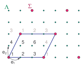
Figure 1: A D2-brane wrapped 6 times around the torus $\mathbb{R}^{2}/\Lambda$ can be represented as a quotient $\mathbb{R}^{2}/\Sigma$ with $\Sigma$ a rank 6 sublattice of $\Lambda$. For the lattice shown here, the classification parameters $m_{ij}$ introduced in the text are $m_{11}=3$, $m_{22}=2$, $m_{21}=1$, $m_{12}=0$. With the indicated sheet labeling $1,\ldots,6$, the closed path $e_{1}$ acts as the permutation $(123)(456)$ on the sheets (so $e_{1}[1]=2$, $e_{1}[2]=3$, $e_{1}[3]=1$ etc.), while $e_{2}$ acts as $(143625)$. From this diagram, one can also read off the winding numbers $\ell_{i}$ that appear further on in the momentum quantization condition: for example the off-diagonal mode generated by $E_{16}$ has $\ell_{1}=2,\ell_{2}=1$.

Consider an arbitrary p-brane wrapped (without branch points) around the torus $T^{p}=\mathbb{R}^{p}/\Lambda$, where $\Lambda=\left\{(i_{1}L_{1},\ldots,i_{p}L_{p})|i_{1},\ldots,i_{p}\in\mathbb{Z}\right\}$. The D-brane, considered as a covering of the torus, can be identified with $\mathbb{R}^{p}/\Sigma$, where $\Sigma$ is a sublattice of $\Lambda$ (see fig 1 for an example). Different possible sublattices correspond to different possible wrappings. Then $N$, the number of times the brane covers the torus is equal to the rank of $\Sigma$ in $\Lambda$, that is, the number of elements in the group $\Lambda/\Sigma$.

The classification of N-fold wrappings is thus equivalent to the classification of sublattices of rank N. A sublattice $\Sigma$ is specified by a basis $\{s_{i}\}_{i}$ with $s_{i}=m_{ij}e_{j}$, where $\{e_{i}\}_{i}$ is the standard basis of $\Lambda$ and $m_{ij}$ is an integral matrix with determinant $N$. Bases that differ by an $SL(p,\mathbb{Z})$ transformation are equivalent as they generate the same lattice $\Sigma$. This equivalence can be used to transform $m_{ij}$ into a lower triangular matrix, i.e. $m_{ij}=0$ for $i<j$. To see this, let us first consider the case $p=2$. An $SL(2,\mathbb{Z})$ transformation acts on $m_{ij}$ as

$$\left(\begin{array}[]{cc}m_{11}&m_{12}\\ m_{21}&m_{22}\end{array}\right)\to\left(\begin{array}[]{cc}a&b\\ c&d\end{array}\right)\left(\begin{array}[]{cc}m_{11}&m_{12}\\ m_{21}&m_{22}\end{array}\right),$$ (6.1)

so in particular $m_{12}\to am_{12}+bm_{22}$. Choosing $a=m_{22}/r$, $b=-m_{12}/r$ with $r=\mbox{gcd}(m_{12},m_{22})$, and $c$, $d$ such that $da-cb=1$ we obtain the desired $SL(2,\mathbb{Z})$ transformation putting $m_{12}=0$. Similarly, for $p>2$, $m_{ij}$ can be put in lower triangular form by repeated application of elements of $SL(2,\mathbb{Z})$ subgroups of $SL(p,\mathbb{Z})$.

Now the residual $SL(p,\mathbb{Z})$ transformations are also lower triangular, with all diagonal elements equal to $\pm 1$. The latter can be taken to be $+1$ by putting all $m_{ii}>0$ (we assume $N>0$, i.e. the brane has positive orientation). The number of times the brane wraps the $x^{i}$ direction is given by $m_{i}\equiv m_{ii}$, and $N=\prod_{i}m_{i}$. The residual equivalence is fixed by requiring $0\leq m_{ij}<m_{ii}$ for all $i,j$ with $i>j$. Indeed, for $p=2$, the residual equivalence acts on $m_{ij}$ as $m_{21}\to m_{21}+c\,m_{11}$, $c\in\mathbb{Z}$ (with the other $m_{ij}$ unchanged), so the equivalence is fixed by requiring $0\leq m_{21}<m_{11}$. For $p>2$, the analogous statement can be deduced by repeated application of the $p=2$ reasoning.

So all in all we find

$$w_{p,N}=\sum_{\{m_{i}\,:\,\prod_{i}m_{i}=N\}}(m_{1})^{p-1}(m_{2})^{p-2}\cdots m_{p-1}$$ (6.2)

inequivalent $N$-fold wrappings of $T^{p}$ by a single $p$-brane, parametrized by $p$ winding numbers $m_{i}$ and $p(p-1)/2$ ‘mixing’ numbers $m_{ij}$, $i>j$.

6.2 Implementation in worldvolume $U(N)$ gauge theory

The low energy dynamics of a Dp-brane wrapped $N$ times around $T^{p}$ is described by a $U(N)$ (Born-Infeld) gauge theory on $T^{p}$ with nontrivial boundary conditions (’t Hooft twists [15]), depending on the structure of the wrapping, which as discussed above is given by a sublattice $\Sigma$ of $\Lambda$. The $U(N)$ indices can be identified with the sheets of the covering $\mathbb{R}^{p}/\Sigma\to\mathbb{R}^{p}/\Lambda$. In general, starting on a sheet $a$ and moving along a closed path $\gamma$ in the torus, one ends up on a different sheet $\gamma[a]$. The sheet permutation $a\to\gamma[a]$ is (up to sheet relabeling) completely determined by $\Sigma$. Indeed, a point on sheet $a$ of the D-brane with coordinate $x$ on $\mathbb{R}^{p}/\Lambda$ is represented by a unique point $x+x(a)$ of the covering space $\mathbb{R}^{p}/\Sigma$. Moving along a closed loop $\gamma$ will move this to the point $x+x(a)+x(\gamma)\mbox{ mod }\Sigma$ of $\mathbb{R}/\Sigma$, which in turn belongs to a certain sheet $\gamma[a]$, uniquely determined by $\Sigma$ (and $\gamma$ of course). Conversely, $\Sigma$ is uniquely determined by the permutations $a\to\gamma[a]$: it is the lattice of points in the covering space $\mathbb{R}^{p}$ reached by paths $\sigma$ that start from $x=0$ and for which $\sigma[a]=a$ for all sheets $a$.

In the case of vanishing background fields, the wrapping structure can be implemented by the following boundary conditions on fields in the fundamental of $U(N)$:

$$\phi(L_{1},x_{2},\ldots,x_{p}) = \Omega_{1}\,\phi(0,x_{2},\ldots,x_{p})$$

$$\phi(x_{1},L_{2},\ldots,x_{p}) = \Omega_{2}\,\phi(x_{1},0,\ldots,x_{p})$$

$$\cdots$$

$$\phi(x_{1},x_{2},\ldots,L_{p}) = \Omega_{p}\,\phi(x_{1},x_{2},\ldots,0),$$

where the $\Omega_{i}$ are the index permutation matrices corresponding to the wrapping structure, that is, identifying the basis element $e_{i}$ of $\Lambda$ with a closed loop in the $x^{i}$ direction:

$${(\Omega_{i})^{a}}_{b}=\delta_{e_{i}[a],b}$$ (6.3)

An equivalent and more invariant description is in terms of parallel transport. Consider an arbitrary path $\gamma$ between points $P_{i}$ and $P_{f}$. Suppose $\gamma$ intersects the coordinate boundary surfaces at the points $P_{1},\ldots,P_{n}$. Then parallel transport of $U(N)$ fundamentals along $\gamma$ is given by $\phi\to U(\gamma)\phi$ with

$$U(\gamma)\equiv\mbox{P}\exp[i\int_{P_{n}}^{P_{f}}A]\,\Omega(P_{n})^{-1}\,\mbox{P}\exp[i\int_{P_{n-1}}^{P_{n}}A]\,\Omega(P_{n-1})^{-1}\cdots\,\mbox{P}\exp[i\int_{P_{i}}^{P_{1}}A],$$ (6.4)

where the path ordered exponentials are over the indicated parts of $\gamma$ and the $\Omega(P_{i})$ are the appropriate $U(N)$ transition functions at the intersection points. On objects $X$ transforming in the adjoint, $U$ acts as $X\to UXU^{-1}$. Note that by construction $U(\gamma_{2}\circ\gamma_{1})=U(\gamma_{2})U(\gamma_{1})$.

Now in the case of zero background field ${\cal A}$, the implementation of the wrapping structure in the gauge theory can be described in terms of $U$ as

$${U(\gamma)^{a}}_{b}=\delta_{\gamma[a],b}$$ (6.5)

for any closed path $\gamma$. In particular for all $\sigma\in\Sigma$ (that is paths starting at 0 and ending at a point of $\Sigma$ when lifted to the covering space $\mathbb{R}^{p}$), we have

$${U(\sigma)^{a}}_{b}=\delta_{a,b}$$ (6.6)

When diagonal background fields are switched on, $U(\gamma)$ and the boundary conditions will in general pick up additional diagonal components (possibly path resp. position dependent), changing (6.5) in

$${U(\gamma)^{a}}_{b}=\delta_{\gamma[a],b}\,e^{i\phi_{b}(\gamma)}.$$ (6.7)

However, parallel transport of a diagonal matrix is insensitive to the phase factors:

$$U(\gamma)\mbox{ diag}(d_{a})_{a}\,U(\gamma)^{-1}=\mbox{ diag}(d_{\gamma[a]})_{a}$$ (6.8)

Note that in general there exist many different equivalent gauge theory descriptions of the same brane system, related by gauge transformations $g(x)$ (not necessarily satisfying the boundary conditions). Such transformations in general change both background fields and boundary conditions. We introduced the description in terms of $U(\gamma)$ here because, unlike boundary conditions and background fields, it is invariant (up to conjugation) under such transformations.

In this paper we only consider backgrounds with diagonal and (covariant) constant field strength ${\cal F}$. This together with (6.8) and the fact that we are considering a single wrapped brane implies that ${\cal F}$ is proportional to the unit matrix $I_{N}$: ${\cal F}=FI_{N}$. Then for a closed contractible path $C$, sweeping out the surface $S$ when contracted to a point, we have

$$U(C)=e^{i\int_{S}F}I_{N},$$ (6.9)

and for two closed paths $\gamma_{1}$, $\gamma_{2}$ with equal base points:

$$U(\gamma_{2})U(\gamma_{1})=e^{i\int_{S(\gamma_{1},\gamma_{2})}F}\,U(\gamma_{1})U(\gamma_{2}),$$ (6.10)

where $S(\gamma_{1},\gamma_{2})$ is the surface swept out by contracting $\gamma_{2}\circ\gamma_{1}\circ\gamma_{2}^{-1}\circ\gamma_{1}^{-1}$. More explicitly, one has

$$\int_{S(\gamma_{1},\gamma_{2})}F=F_{ij}\int_{\gamma_{1}}dx^{i}\,\int_{\gamma_{2}}dx^{j}.$$ (6.11)

Since $U(\sigma)$ is diagonal for $\sigma\in\Sigma$ (cf. equation (6.7)), the relation (6.10) implies that for $\sigma_{1},\sigma_{2}\in\Sigma$ we must have

$$F_{ij}\int_{\sigma_{1}}dx^{i}\,\int_{\sigma_{2}}dx^{j}\in 2\pi\mathbb{Z}.$$ (6.12)

Applying this to the basis elements $s_{i}=m_{ij}e_{j}$ of $\Sigma$ introduced in section 6.1, yields the flux quantization condition

$$F_{ij}=\frac{2\pi}{L_{i}L_{j}}(m^{-1})_{ik}\,(m^{-1})_{jl}\,q_{kl}$$ (6.13)

where the $q_{kl}=-q_{lk}$ are integers.

Note also that parallel transport of objects transforming in the adjoint is invariant under continuous path deformations.

6.3 Fluctuation spectrum

Because the field strength is proportional to the unit matrix, the derivation of the fluctuation spectrum of the non-abelian Born-Infled theory in this background is quite analogous to the derivation in the abelian $U(1)$ case discussed in section 2. The main difference is the modified quantization condition on the momenta. When the brane carries flux, this modification is nontrivial [6]. Below we give a general construction of the spectrum, independent of specific background field and boundary condition choices, which clearly shows the physical origin of the modifications to the momentum quantization condition.

The fluctuation modes of the quadratic Lagrangian (3.9), in the gauge $A_{0}=0$, $D_{i}A^{i}=0$, are of the form $\delta A_{i}=u_{i}\delta A$ with $k^{i}u_{i}=0$ and $\delta A$ a solution of

$$D_{j}\delta A=ik_{j}\delta A,$$ (6.14)

with energy

$$M^{2}={\cal G}^{ij}k_{i}k_{j}$$ (6.15)

where ${\cal G}$ is given by (2.4) as usual. Solutions to (6.14) are of the form

$$\delta A(x)=U(\gamma_{x})\,\delta A_{0}\,U(\gamma_{x})^{-1}\,e^{i\int_{\gamma_{x}}k_{i}dx^{i}},$$ (6.16)

where $\gamma_{x}$ is any path from 0 to $x$. Because $U$ acting in the adjoint is invariant under continuous path deformations, (6.16) gives indeed a well defined globally smooth solution, provided

$$\delta A_{0}=U(\lambda)\,\delta A_{0}\,U(\lambda)^{-1}\,e^{i\int_{\lambda}k_{i}dx^{i}}$$ (6.17)

for any closed path $\lambda$ based at $0$. Such paths can be identified with the points of the lattice $\Lambda$, hence the notation $\lambda$. Note that if condition (6.17) is satisfied, one trivially has

$$\delta A_{0}=\lim_{\Lambda^{\prime}\to\Lambda}\frac{1}{|\Lambda^{\prime}|}\sum_{\lambda^{\prime}\in\Lambda^{\prime}}U(\lambda^{\prime})\,\delta A_{0}\,U(\lambda^{\prime})^{-1}\,e^{i\int_{\lambda^{\prime}}k_{i}dx^{i}},$$ (6.18)

where $\Lambda^{\prime}$ denotes a subset of $\Lambda$ of size $|\Lambda^{\prime}|$. Conversely, any $\delta A_{0}$ defined by

$$\delta A_{0}\equiv\langle E\rangle_{k}\equiv\lim_{\Lambda^{\prime}\to\Lambda}\frac{1}{|\Lambda^{\prime}|}\sum_{\lambda^{\prime}\in\Lambda^{\prime}}U(\lambda^{\prime})\,E\,U(\lambda^{\prime})^{-1}\,e^{i\int_{\lambda^{\prime}}k_{i}dx^{i}},$$ (6.19)

with $E$ an arbitrary matrix, automatically satisfies condition (6.17), as follows from $U(\lambda)U(\lambda^{\prime})=U(\lambda\circ\lambda^{\prime})$ and invariance up to a phase of (6.18) under the shift $\lambda^{\prime}\to\lambda\circ\lambda^{\prime}$.

So the general solution to (6.17) is a linear combination of the matrices $\langle E_{ab}\rangle_{k}$, with the matrix basis $E_{ab}$, $a,b=1,\ldots,N$ as defined under equation (3.13). Now $\langle E_{ab}\rangle_{k}$ is only nonzero for specific values of the momentum $k$. To see this, first note that (6.7) implies we can write $E_{ab}=U(\gamma_{ab})D_{b}$ with $\gamma_{ab}$ a closed path that, lifted to the covering space, runs from 0 lifted to sheet $a$ to 0 lifted to sheet $b$, so $\gamma_{ab}[a]=b$, and with $D_{b}$ the diagonal matrix defined by $(D_{b})_{cc}=e^{-i\phi_{b}(\gamma_{ab})}\delta_{cb}$. Then for $\sigma\in\Sigma$, we have

$$\langle E_{ab}\rangle_{k} = \langle U(\gamma_{ab})D_{b}\rangle_{k}$$

$$= \exp[i\int_{\sigma}k_{i}dx^{i}]\,\langle U(\sigma)U(\gamma_{ab})\,D_{b}\,U(\sigma)^{-1}\rangle_{k}$$

$$= \exp[i\int_{\sigma}k_{i}dx^{i}]\,\langle\exp[i\int_{S(\gamma_{ab},\sigma)}F]\,U(\gamma_{ab})U(\sigma)\,D_{b}\,U(\sigma)^{-1}\rangle_{k}$$

$$= \exp[i\int_{\sigma}k_{i}dx^{i}+i\int_{S(\gamma_{ab},\sigma)}F]\,\langle U(\gamma_{ab})\,D_{b}\,\rangle_{k}$$

$$= \exp[i\int_{\sigma}k_{i}dx^{i}+i\int_{S(\gamma_{ab},\sigma)}F]\,\langle E_{ab}\rangle_{k}.$$

Equation (6.10) was used in going from the second to the third line, and (6.8) together with $\sigma[b]=b$ to go from the third line to the fourth. So $\langle E_{ab}\rangle_{k}$ can only be nonzero if the following momentum quantization condition is satisfied:

$$\int_{\sigma}k_{i}dx^{i}+\int_{S(\gamma_{ab},\sigma)}F\in 2\pi\mathbb{Z}$$ (6.20)

for all $\sigma\in\Sigma$. For diagonal excitations, the flux term is zero and the quantization condition is simply the usual one for a particle on a compact space — here the covering space $\mathbb{R}^{p}/\Sigma$ corresponding to the wrapped brane, as could be expected. However, off-diagonal excitations pick up an additional phase when going around a loop, and the quantization condition is shifted. In the string picture of these excitations, where the off-diagonal fluctuations correspond to open strings with endpoints on different sheets, this additional term is easily understood: it is nothing but the usual coupling of a string running from sheet $a$ to sheet $b$ and going around a loop $\sigma$ of the brane, to the given gauge field background. Also the effective metric ${\cal G}$ appearing in (6.15) can be understood directly in the string theory picture, see e.g. [16]. So here the non-abelian Born-Infeld theory matches nicely with string theory expectations, and in particular we expect the fluctuation spectrum to be reproduced by string theory on an appropriate T-dual system, as in [6], though we did not work out the details for the general case.

Let us make (6.20) more explicit. Using (6.11) and (6.13), and taking $\sigma$ equal to the basis elements $s_{i}=m_{ij}e_{j}$ introduced in section 6.1, the quantization condition can be rewritten as

$$k_{i}=\frac{2\pi}{L_{i}}(m^{-1})_{ij}\,[n_{j}+(m^{-1})_{kl}\,q_{jl}\,\ell_{k}],$$ (6.21)

where the $n_{j}$ are arbitrary integers, $q_{jl}=-q_{lj}$ are the flux quantum numbers from (6.13), and $\ell_{k}$ is the winding number of $\gamma_{ab}$ in the $x^{k}$ direction: $\gamma_{ab}=l_{k}e_{k}$. The precise fractionalization of momentum depends on the details of the different integers involved, but the minimal momentum quantum will never be less than $1/N$.

Note that if the momentum quantization condition is satisfied, the infinite sum in (6.19) can be reduced to a finite sum over $\Lambda/\Sigma$:

$$\langle E_{ab}\rangle_{k}=\frac{1}{N}\sum_{\lambda^{\prime}\in\Lambda/\Sigma}U(\lambda^{\prime})\,E_{ab}\,U(\lambda^{\prime})^{-1}\,e^{i\int_{\lambda^{\prime}}k_{i}dx^{i}},$$ (6.22)

because paths $\lambda^{\prime}$ and $\lambda^{\prime}\circ\sigma$, with $\sigma\in\Sigma$, give the same contribution. This gives an in principle straightforward way to compute the $\langle E_{ab}\rangle_{k}$ explicitly for a given $U(N)$ bundle. It also shows that all modes constructed from $\langle E_{ab}\rangle_{k}$ are nonzero, because all terms in the finite sum are linearly independent matrices. Finally note that all $\langle E_{ab}\rangle_{k}$ with the same $\gamma_{ab}$ (i.e. the same $\ell_{i}$) are actually equal up to a phase factor, as they are mapped to each other by a path shift $\lambda^{\prime}\to\lambda^{\prime}\circ\gamma$ for a certain $\gamma$. This corresponds to the fact that only the relative position (in the covering space) of the sheets is physical. So the quantum numbers $n_{i}$ and $\ell_{i}$ appearing in (6.21) label the modes without degeneracy.

7 Conclusions

The calculation of the mass spectrum is probably the simplest question which can be addressed by means of the effective action. It only probes the effective action through second order in the fluctuations. As we demonstrated in this paper, the non-abelian Born-Infeld action defined using the symmetrized trace prescription is not able to reproduce the spectrum as predicted by string theory. Not surprisingly, the first two terms of the Born-Infeld action, the $F^{2}$ and $F^{4}$ terms, give correct answers. However at order $F^{6}$ and higher, things go wrong. Keeping in mind that the non-abelian Born-Infeld action should reduce to the sum of abelian Born-infeld actions for well separated D-branes, additional corrections should involve commutators of the field strengths. As advocated by Tseytlin, this can be understood as follows. At higher order one expects corrections going as derivatives acting on the fieldstrength [14] which, under the assumption that the velocities vary slowly, are ignored in the effective action. However this is ambiguous in a non-abelian gauge theory as one has that

$$D_{\alpha}D_{\beta}F_{\gamma\delta}=\frac{1}{2}\{D_{\alpha},D_{\beta}\}F_{\gamma\delta}-\frac{i}{2}{[}F_{\alpha\beta},F_{\gamma\delta}{]}.$$ (7.1)

It is clear that the symmetrized product of derivatives acting on a fieldstrength should be viewed as an acceleration term which can safely be neglected. The anti-symmetrized products however should be kept and will contribute to the mass spectrum! Precisely these terms are not captured by the proposal in [5].

The present work clearly demonstrates the need to address this problem. One possible way would be to construct these terms using string field theory along the lines developed in [17]. However in order to make concrete statements about the $F^{6}$ terms, the calculation has to be pushed to an order which is probably unfeasible without the aid of a computer. Another way to get the $F^{6}$ terms would be by calculating a five loop beta function. Due to the fact that for the present purpose it is sufficient to consider trivial gravitational backgrounds, the vertices appearing are rather simple. Despite of this, the calculation remains very involved. Yet another approach could consist of supersymmetrizing the non-abelian Born-Infeld action. It might be that the requirement of invariance under $\kappa$-symmetry favorizes certain ordenings.

Perhaps the simplest way to proceed is by using the mass spectrum as a guideline. As a first step, one would have to make a systematic analysis of possible modifications of the $F^{6}$ terms in the non-abelian Born-Infeld action. In [8], a first attempt was already made but it was clear that the $T^{4}$ case was not sufficient to unambigously determine the $F^{6}$ term. Now, many more examples are available. A priori we expect 5! different permutations of the Lie algebraic factors to be relevant. However, as the mass spectrum automatically narrows the group to a $U(2)$ factor, the number of truly inequivalent permutations is considerably smaller. In fact a closer analysis shows that there are only 15 possibilities. Furthermore, ignoring the Lorentz indices all together, only 5 inequivalent ordenings remain. The two-torus, being a particularly simple case, is the best place to start the analysis.

Additional hints are provided by the BPS configurations on $T^{4}$ for which Tseytlins prescription does provide the correct spectrum. On $T^{6}$ and $T^{8}$ further insights are provided by the fact that in the Yang-Mills case BPS configurations involve linear relations between the backgrounds [10], while for the Born-Infeld theory the backgrounds should satisfy non-linear relations [11]. Indeed, focussing on $T^{6}$ we saw that at the level of the Yang-Mills theory the BPS relation is given by $f_{1}-f_{2}-f_{3}=0$ while in the Born-Infeld theory it becomes

$$f_{1}-f_{2}-f_{3}=(2\pi\alpha^{\prime})^{2}f_{1}f_{2}f_{3}.$$ (7.2)

We reinserted the factors of $2\pi\alpha^{\prime}$ in order to clearly demonstrate that this indeed relates different orders in $F$ in the Born-Infeld theory.

We also know that the Born-Infeld spectrum should have the same form as the Yang-Mills spectrum, but with rescaled backgrounds. As became clear from section 5, this puts strong additional constraints on the possible modifications. Finally, requiring a consistent behaviour of the Born-Infeld action under T-duality further reduces the possibilities. A systematic study of modifications of the non-abelian Born-Infeld action satisfying all requirements will be presented in a separate publication [18].

The initial exploration of general wrappings of D-branes on tori, opens several interesting questions, such as the precise implications of T-duality transformations and D-brane configurations on more involved geometries, which deserve further investigation. We hope to return to this in the future.

Acknowledgments: We would like to thank Walter Troost for several illuminating discussions and Alberto Santambrogio for a useful comment. A.S. and J.T. are supported in part by the FWO and by the European Commission TMR programme ERBFMRX-CT96-0045 in which both are associated to K. U. Leuven.

References

• [1] Good reviews on the subject can be found in W. Taylor, Lectures on D-Branes, Gauge Theory and M(atrices), lectures presented at the Trieste summer school on particle physics and cosmology, June 1997, hep-th/9801182; J. Polchinski, TASI lectures on D-branes, hep/th9611050 and A. A. Tseytlin, Born-Infeld Action, Supersymmetry and String Theory, to appear in the Yuri Golfand memorial volume, hep-th/9908105
• [2] E. Witten, Nucl. Phys. B460 (1996) 35, hep-th/9510135
• [3] D. J. Gross and E. Witten, Nucl. Phys. B277 (1986) 1; A.A. Tseytlin, Nucl. Phys. B276 (1986) 391 and Nucl. Phys. B291 (1987) 876.
• [4] D. Brecher and M.J. Perry, Nucl. Phys. B527 (1998) 121, hep-th/9801127; K. Behrndt, Open Superstring in Non-Abelian Gauge Field, in the procs. of the XXIII Int. Symp. Ahrenshoop 1989, 174, Akademie der Wissenschaften der DDR; Untersuchung der Weyl-Invarianz im Verallgemeinter $\sigma$-Modell fΓΌr Offene Strings, PhD thesis, Humboldt-UniversitΓ€t zu Berlin, 1990
• [5] A.A. Tseytlin, Nucl. Phys. B501 (1997) 41, hep-th/9701125
• [6] A. Hashimoto and W. Taylor, Nucl. Phys. B503 (1997) 193, hep-th/9703217
• [7] Z. Guralnik and S. Ramgoolam, Nucl. Phys. B499 (1997) 241, hep-th/9702099; Nucl. Phys. B521 (1998) 129, hep-th/9708089
• [8] P. Bain, On the Non-Abelian Born-Infeld Action, to appear in the proceedings of the CargΓ¨se ’99 Summer School, hep-th/9909154
• [9] P. van Baal, Comm. Math. Phys. 94 (1984) 397 and 85 (1982) 529
• [10] J. Troost, Constant Field Strengths on $T^{2n}$, to appear in Nucl. Phys. B, hep-th/9909187
• [11] M. Berkooz, M. R. Douglas and R. Leigh, Nucl. Phys. B480 (1996) 265, hep-th/9606139
• [12] A. Abouelsaood, C. Callan, C. Nappi and S. Yost, Nucl. Phys. B280 (1987) 599
• [13] M. Costa and M. Perry, Nucl. Phys. B524 (1998) 333, hep-th/9712160; Nucl. Phys. B520 (1998) 205, hep-th/9712026
• [14] O. D. Andreev and A. A. Tseytlin, Nucl. Phys. B311 (1988) 205
• [15] G. ’t Hooft, Comm. Math. Phys. 81 (1981) 267
• [16] N. Seiberg and E. Witten, JHEP 9909 (1999) 032, hep-th/9908142
• [17] W. Taylor, preprint, D-Brane Effective Field Theory from String Field Theory, hep-th/0001201
• [18] A. Sevrin, J. Troost and W. Troost, work in progress