Abstract

A continuum of monopole, dyon and black hole solutions exist in the Einstein-Yang-Mills theory in asymptotically anti-de Sitter space. Their structure is studied in detail. The solutions are classified by non-Abelian electric and magnetic charges and the ADM mass. The stability of the solutions which have no node in non-Abelian magnetic fields is established. There exist critical spacetime solutions which terminate at a finite radius, and have universal behavior. The moduli space of the solutions exhibits a fractal structure as the cosmological constant approaches zero.

1 Introduction

For a long time, it was believed that no regular particle-like stable solutions (solitons) with finite mass can exist in self gravitating systems unless the stability is guaranteed topologically. The Einstein theory in vacuum and the Einstein-Maxwell system do not admit solitons. It came as quite a surprise when Bartnik and McKinnon (BK) found globally regular solutions to the $SU(2)$ Einstein Yang-Mills (EYM) theory without scalar fields[1]. It was unexpected to find that self gravitating Yang-Mills systems produced solitons. Unfortunately, the BK solutions were shown to be unstable against linear perturbations [2]. Later, other fields such as Higgs scalar fields and dilaton fields were included in the EYM action, but with the exception of the Skyrmions, all turned out to be unstable (see [3] for a review).

Interest in the BK solutions was renewed with the discovery of black hole solutions to the EYM equations [4, 5]. These non-Abelian black holes aparently violate the no-hair conjecture [6]. But these non-Abelian black hole solutions are also unstable, and again other fields were added in the hope of achieving stability without success (see Ref.’s [3, 7]) for a review).

We stress that it is a surprise that there are static solutions to the Einstein Yang-Mills equations at all. There are no static solutions to the Yang-Mills equations in 4 dimensional flat space. We can see this with a simple argument given by Deser [8]. The conservation of the canonical energy momentum tensor, $\partial_{\nu}T^{\mu\nu}=0$, implies that for a static field configuration $\partial_{j}{T_{i}}^{j}=0$. The total divergence of the quantity $x^{i}{T_{i}}^{j}$ must vanish to maintain finite energy and regularity, $\int d^{d-1}x\partial_{j}(x^{i}{T_{i}}^{j})=0$. But $\partial_{j}(x^{i}{T_{i}}^{j})={T_{j}}^{j}+x^{i}\partial_{j}{T_{i}}^{j}={T_{j}}^{j}$ so that

$$\int d^{d-1}x~{}T^{i}_{i}=\int d^{d-1}x\left[\frac{1}{2}(5-d)F^{2}_{ij}+(d-3)F^{2}_{0i}\right]=0.$$ (1)

Since the integrand above is positive definite for $d=4$, $F_{ij}$ and $F_{0i}$ must vanish. Thus there are no regular static solutions.

The argument above cannot be extended to curved spacetime. The conservation law ${T^{\mu\nu}}_{;\nu}=0$ leads to

$$\int d^{d-1}x\,\sqrt{-g}~{}{T_{j}}^{j}=-\int d^{d-1}x\,\sqrt{-g}~{}x^{k}~{}\Gamma_{k\mu\nu}T^{\mu\nu}\not=0~{}.$$ (2)

The failure of Deser’s simple argument in curved space implies the possibility of having static solutions in curved space. Gravity supplies the attractive force needed to balance the repulsive force of Yang-Mills gauge interactions. Indeed, any solution to $SU(2)$ EYM equations in asymptotically Minkowski space which is regular asymptotically is also regular for all $r>0$ [9].

The particle-like and black hole solutions were later studied in a cosmological context. The behavior of static solutions to the Einstein Yang-Mills equations depends considerably on the sign of the cosmological constant. The solutions can be separated into two families; $\Lambda\geq 0$ and $\Lambda<0$. The solutions where $\Lambda=0$ are the BK solutions. Their asymptotically de Sitter analogs ($\Lambda>0$) were discovered independently by Volkov et. al. and Torii et. al. [10]. The BK solutions and the cosmological extensions all share similar behavior, and are unstable [11, 12]. (See Ref. [3] for a review). Recently, asymptotically anti-de Sitter black hole solutions [13] and soliton solutions [14, 15] were found which are strikingly different from the BK type solutions. In particular, the asymptotically anti-de Sitter AdS EYM equations have solutions where the field strengths are non-zero everywhere. These solutions were also shown to be stable against spherically symmetric linear perturbations. These solutions are the only EYM solutions solutions that are stable. This discovery would be very important to cosmology if the universe was ever in a phase where the cosmological constant is negative.

Another new feature of the EYM theory in AdS is the existence of dyon solutions. If $\Lambda\geq 0$ the electric part of the gauge fields is forbidden [16] if the ADM mass is to remain finite. Scalar fields must be added to the theory in order for the boundary conditions at infinity to permit the electric fields and maintain a finite ADM mass [18, 19].

Recently a tremendous amount of interest has evolved in field theories in AdS space. There is the AdS/CFT correspondence [17]. Conformal field theories in $d$ dimensions ($R_{d}$) are described in terms of supergravity or string theory on the product space of AdS_d+1 and a compact manifold. There are intimate relations between data on the boundary $R_{d}$ of AdS_d+1 and data in the bulk AdS_d+1. In the present paper we are examining the Einstein-Yang-Mills theory in asymptotically AdS space. The boundary in space must be playing a crucial role for the existence of stable monopole and dyon solutions, more detailed analysis of which is, however, left for future investigation. We also note that in the three-dimensional AdS space there exist nontrivial black holes [20] and monopole/instanton solutions [21].

When the value of the cosmological constant $\Lambda$ is varied, the space of monopole and dyon solutions, the moduli space, also changes. With a finite negative $\Lambda$, solutions exist in continuum. They are classified in a finite number of families, or branches. With a vanishing or positive $\Lambda$ solution exists only in a discrete set, but there are infinitely many. One natural question emerging is how these finite number of branches of solutions in continuum become infinitely many discrete points as $\Lambda<0$ approaches 0. There is a surprising hidden feature in this limit. We shall find a fractal structure in the moduli space, which seems to explain the transition.

In the next section the general formalism is given and the equations of motion are derived with a spherically symmetric ansatz. Conserved charges in the Yang-Mills theory is defined in section 3. Some general no-go theorems are derived from sum rules in Section 4. New soliton solution in asymptotically anti-de Sitter space are explained in section 5. The critical spacetime which have universality near the edge of the space is also examined. Black hole solutions which have both magnetic and electric non-Abelian charges are presented in Section 6. The dependence of the moduli space on the cosmological constant $\Lambda$ is investigated in Section 7 where the fractal structure is revealed when $\Lambda$ approaches zero from the negative side. The detailed analysis of the stability of the monopole solutions is presented in Section 8. The subtle boundary condition in the problem requires elaboration of the previous argument presented in the $\Lambda=0$ and $\lambda>0$ cases.

2 General Formalism

In non-Abelian gauge theory, the field equations have solutions which exhibit a magnetic charge. In the ’t Hooft-Polyakov monopole solution

$$\begin{array}[]{lcr}\Phi_{a}={\displaystyle x_{a}\over\displaystyle er^{2}}H(er),&A_{a}^{0}=0,&A^{i}_{a}=-\epsilon_{aij}{\displaystyle x_{j}\over\displaystyle er^{2}}(1-K(er)).\end{array}$$ (3)

where $\Phi_{a}$ is a triplet Higgs scalar field. Its stability is guaranteed by the topology of the triplet Higgs scalar field.[22] The $U(1)$ magnetic charge takes a quantized value, $4\pi/e$. Dyon solutions were obtained [23] starting with the above ansatz (3) but with a non-zero value for $A_{a}^{0}$, (i.e. $A_{a}^{0}=(x_{a}/er^{2})J(er)$).

In this paper we look for monopole and dyon solutions in the Einstein-Yang-Mills theory without scalar fields;

$$S=\int d^{4}x\sqrt{-g}\left[\frac{1}{16\pi G}(R-2\Lambda)-{1\over 4}F^{a\mu\nu}{F^{a}}_{\mu\nu}\right].$$ (4)

The Einstein and Yang-Mills equations are given by

$$R^{\mu\nu}-{1\over 2}g^{\mu\nu}(R-2\Lambda)=8\pi G~{}T^{\mu\nu}$$ (5)

$${F^{\mu\nu}}_{;\mu}+e[A_{\mu},F^{\mu\nu}]=0$$ (6)

We suspect that the gravity provides attractive force to balance the equation.

We look for spherically symmetric solutions. The metric takes the form

$$ds^{2}=-{\displaystyle H\over\displaystyle p^{2}}\,dt^{2}+{\displaystyle dr^{2}\over\displaystyle H}+r^{2}(d\theta^{2}+\sin^{2}\theta\,d\phi^{2})$$ (7)

whereas Yang-Mills fields are given [24, 25], in the regular gauge, by

$$A^{(0)} = {\tau^{j}\over 2e}\Bigg{\{}{A_{0}}{x_{j}\over r}dt+{A_{1}}{x_{j}x_{k}\over r^{2}}dx_{k}$$ (9)

$$\hskip 19.91684pt+{\phi_{1}\over r}\bigg{(}\delta_{jk}-{x_{j}x_{k}\over r^{2}}\bigg{)}dx_{k}-\epsilon_{jkl}{1-\phi_{2}\over r^{2}}{x_{k}}dx_{l}\Bigg{\}}$$

Here the Cartesian coordinate $x^{k}$’s are related to the polar coordinates $(r,\theta,\phi)$ as in the flat space. $H$, $p$, $A_{0}$, $A_{1}$, $\phi_{1}$ and $\phi_{2}$ are functions of $r$ for monopole or dyon solutions. In the discussion of the stability of the solutions they depend on both $t$ and $r$. The regularity of solutions at the origin demands that $H$, $p$ are finite, whereas $A_{0}$, $A_{1}$, and $\phi_{1}\rightarrow 0$ and $\phi_{2}\rightarrow 1$ at $r=0$.

2.1 Simplification of the static gauge field ansatz

Let $A=A_{\mu}dx^{\mu}=\frac{1}{2}\tau^{a}A_{\mu}^{a}dx^{\mu}$, where $\tau^{a}$ are the usual Pauli matrices. In terms of the basis in spherical coordinates $(\tau_{r},\tau_{\theta},\tau_{\phi})=(\vec{n}_{r},\vec{n}_{\theta},\vec{n}_{\phi})\vec{\tau}$ which satisfies $[\tau_{i},\tau_{j}]=2i\epsilon_{ijk}\tau_{k}$ ($i=r,\theta,\phi$), the ansatz (9) is written as

$$A^{(0)}=\frac{1}{2e}\Big{[}A_{0}\tau_{r}dt+A_{1}\tau_{r}dr+(\phi_{1}\tau_{\theta}+(\phi_{2}-1)\tau_{\phi})d\theta$$ (10)

$$+(-(\phi_{2}-1)\tau_{\theta}+\phi_{1}\tau_{\phi})\sin\theta d\phi\Big{]}$$ (11)

Note that there are no singularities in this gauge. Next make a gauge transformation $A=SA^{(0)}S^{-1}-(i/e)dS\cdot S^{-1}$ where

$$S=\left(\matrix{+e^{i(\phi+\Omega)/2}\cos{\displaystyle\theta\over\displaystyle 2}&~{}~{}+e^{-i(\phi-\Omega)/2}\sin{\displaystyle\theta\over\displaystyle 2}\cr-e^{i(\phi-\Omega)/2}\sin{\displaystyle\theta\over\displaystyle 2}&~{}~{}+e^{-i(\phi+\Omega)/2}\cos{\displaystyle\theta\over\displaystyle 2}\cr}\right)~{}~{},~{}~{}\Omega=\Omega(t,r)~{}~{}.$$ (12)

Useful identities are

$$S\tau_{r}S^{-1} = \tau_{3}$$ (13)

$$S\tau_{\theta}S^{-1} = \cos\Omega\tau_{1}-\sin\Omega\tau_{2}$$ (14)

$$S\tau_{\phi}S^{-1} = \sin\Omega\tau_{1}+\cos\Omega\tau_{2}$$ (15)

$$2idS\cdot S^{-1} = -(\Omega^{\prime}dr+\dot{\Omega}dt)\tau_{3}-d\theta(\sin\Omega\tau_{1}+\cos\Omega\tau_{2})$$ (17)

$$+d\phi(\sin\theta\cos\Omega\tau_{1}-\sin\theta\sin\Omega\tau_{2}-\cos\theta\tau_{3})$$

The new gauge potential is

$$A=\frac{1}{2e}\,\Big{\{}u\tau_{3}dt+\nu\tau_{3}dr+(w\tau_{1}+\tilde{w}\tau_{2})d\theta+(\cot\theta\tau_{3}+w\tau_{2}-\tilde{w}\tau_{1})\sin\theta d\phi\Big{\}}.$$ (18)

where

$$u = A_{0}+\dot{\Omega}$$ (19)

$$\nu = A_{1}+\Omega^{\prime}$$ (20)

$$w = +\phi_{1}\cos\Omega+\phi_{2}\sin\Omega$$ (21)

$$\tilde{w} = -\phi_{1}\sin\Omega+\phi_{2}\cos\Omega~{}~{}~{}.$$ (22)

Note that the gauge transformation (12) is singular at $\theta=0$ and $\pi$. Eq. (22) is the gauge potential in the singular gauge. It has a Dirac string. One can always choose $\Omega(t,r=0)=\pi/2$ with which the boundary conditions at $r=0$ are $u=\nu=\tilde{w}=0$ and $w=1$. With appropriate $\Omega(t,r)$ one can set $\nu(t,r)=0$ or $u(t,r)=0$.

A straightforward calculation leads to the field strength $F=dA-ieA\wedge A$:

$$F = \frac{1}{2e}\bigg{\{}(\dot{\nu}-u^{\prime})\tau_{3}dt\wedge dr+\Big{[}(\dot{w}-u\tilde{w})\tau_{1}+(\dot{\tilde{w}}+uw)\tau_{2}\Big{]}dt\wedge d\theta$$ (27)

$$\hskip 28.45274pt-\Big{[}(uw+\dot{\tilde{w}})\tau_{1}+(u\tilde{w}-\dot{w})\tau_{2}\Big{]}dt\wedge\sin\theta d\phi$$

$$\hskip 28.45274pt+\Big{[}(w^{\prime}-\nu\tilde{w})\tau_{1}+(\tilde{w}^{\prime}+w\nu)\tau_{2}\Big{]}dr\wedge d\theta$$

$$\hskip 28.45274pt+\Big{[}(w^{\prime}-\nu\tilde{w})\tau_{2}+(-\tilde{w}^{\prime}-\nu w)\tau_{1}\Big{]}dr\wedge\sin\theta d\phi$$

$$\hskip 28.45274pt-(1-w^{2}-\tilde{w}^{2})\tau_{3}d\theta\wedge\sin\theta d\phi\bigg{\}}~{}~{}.$$

The configurations where $\nu=u=0$, $w=\tilde{w}=$constant, and $w^{2}+\tilde{w}^{2}=1$ are pure gauge.

2.2 Equations of motion

In the general spherically symmetric metric (7) tetrads are

$$e_{0}={\sqrt{H}\over p}dt~{}~{}~{},~{}~{}~{}e_{1}={1\over\sqrt{H}}dr~{}~{}~{},~{}~{}~{}e_{2}=rd\theta~{}~{}~{},~{}~{}~{}e_{3}=r\sin\theta d\phi~{}~{}~{}.$$ (28)

In the tetrad basis $F_{ab}=(e_{a})_{\mu}(e_{b})_{\nu}F^{\mu\nu}$ and the energy-momentum tensors are $T_{ab}=F_{ac}^{(i)}F_{b}^{c(i)}-\frac{1}{4}\eta_{ab}F_{de}^{(i)}F^{de(i)}$. The nonvanishing components of the Yang-Mills equations (6) are

$$\left(pr^{2}(u^{\prime}-\dot{\nu})\right)^{\prime}-2\frac{p}{H}\big{\{}w(uw+\dot{\tilde{w}})+\tilde{w}(u\tilde{w}-\dot{w})\big{\}}=0$$ (29)

$$\left(pr^{2}(u^{\prime}-\dot{\nu})\right)_{,\;t}-2\frac{H}{p}\big{\{}-\tilde{w}w^{\prime}+\tilde{w}^{\prime}w+\nu(w^{2}+\tilde{w}^{2})\big{\}}=0$$ (30)

$$\left(\frac{H}{p}(w^{\prime}-\tilde{w}\nu)\right)^{\prime}-\left({p\over H}(\dot{w}-u\tilde{w})\right)_{,\;t}$$ (31)

$$\hskip 56.9055pt+\frac{p}{H}u(uw+\dot{\tilde{w}})+\frac{w(1-w^{2}-\tilde{w}^{2})}{pr^{2}}-\frac{H}{p}\nu(\tilde{w}^{\prime}+w\nu)=0$$ (32)

$$\left(\frac{H}{p}(\tilde{w}^{\prime}+w\nu)\right)^{\prime}-\left({p\over H}(\dot{\tilde{w}}+uw)\right)_{,\;t}$$ (33)

$$\hskip 56.9055pt+\frac{p}{H}u(u\tilde{w}-\dot{w})+\frac{\tilde{w}(1-w^{2}-\tilde{w}^{2})}{pr^{2}}+\frac{H}{p}\nu(w^{\prime}-\tilde{w}\nu)=0~{}~{}.\hskip 28.45274pt$$ (34)

The nonvanishing components of the energy-momentum tensor are given by

$$T_{00} = {1\over e^{2}}(A+B)$$ (35)

$$T_{11} = {1\over e^{2}}(-A+B)$$ (36)

$$T_{22} = T_{33}={1\over e^{2}}A$$ (37)

$$T_{01} = -{1\over e^{2}}\,C$$ (38)

where

$$A = {1\over 2}\,p^{2}(\dot{\nu}-u^{\prime})^{2}+{1\over 2r^{4}}\,(1-w^{2}-\tilde{w}^{2})^{2}$$ (39)

$$B = {p^{2}\over r^{2}H}\Big{\{}(uw+\dot{\tilde{w}})^{2}+(\dot{w}-u\tilde{w})^{2}\Big{\}}+{H\over r^{2}}\Big{\{}(w^{\prime}-\nu\tilde{w})^{2}+(\tilde{w}^{\prime}+\nu w)^{2}\Big{\}}$$ (40)

$$C = {2p\over r^{2}}\Big{\{}(\tilde{w}^{\prime}+\nu w)(uw+\dot{\tilde{w}})+(w^{\prime}-\nu\tilde{w})(\dot{w}-u\tilde{w})\Big{\}}~{}~{}.$$ (41)

The Einstein equations reduce to

$${p^{\prime}\over p}=-{8\pi G\over e^{2}}~{}{rB\over H}$$ (42)

$$-{H^{\prime}\over r}+{1-H\over r^{2}}={8\pi G\over e^{2}}~{}(A+B)+\Lambda$$ (43)

$${p\over 2}\Bigg{\{}\bigg{(}{p\dot{H}\over H^{2}}\bigg{)}_{,t}+\bigg{(}{pH^{\prime}-2p^{\prime}H\over p^{2}}\bigg{)}^{\prime}\Bigg{\}}+{1-H\over r^{2}}={16\pi G\over e^{2}}\,A$$ (44)

$${p\dot{H}\over rH}=-{8\pi G\over e^{2}}\,C$$ (45)

It is convenient to introduce $m(r)$ defined by

$$H(r)=1-{2m(r)\over r}-{\Lambda r^{2}\over 3}~{}~{}.$$ (46)

$m(r)$ is the mass contained inside the radius $r$. $p(r)=$constant and $m(r)=0$ corresponds to the Minkowski, de Sitter, or anti-de Sitter space for $\Lambda=0,>0,$ or $<0$, respectively. Then the second equation in (45) becomes

$$m^{\prime}={4\pi G\over e^{2}}\,r^{2}(A+B)~{}~{}.$$ (47)

The system of the Einstein-Yang-Mills equations contains one redundant equation. The third equation in (45) follows from (34) and the rest of (45).

2.3 Static configurations

It is most convenient to take the $\nu=0$ gauge for static configurations. The second equation in (34) then yields $w\tilde{w}^{\prime}-w^{\prime}\tilde{w}=0$, which leads to $\tilde{w}(r)=Cw(r)$. By a further global rotation $\Omega=$constant in (22) one can set $\tilde{w}=0$. As a result

$$A = \frac{1}{2e}\Big{\{}u\tau_{3}dt+w\tau_{1}d\theta+(\cot\theta\tau_{3}+w\tau_{2})\sin\theta d\phi\Big{\}}$$ (48)

$$F = \frac{1}{2e}\bigg{\{}-u^{\prime}\tau_{3}dt\wedge dr+uwdt\wedge(\tau_{2}d\theta-\tau_{1}\sin\theta d\phi)$$ (50)

$$\hskip 28.45274pt+w^{\prime}dr\wedge(\tau_{1}d\theta+\tau_{2}\sin\theta d\phi)-(1-w^{2})\tau_{3}d\theta\wedge\sin\theta d\phi\bigg{\}}~{}~{}.$$

Then the Einstein-Yang-Mills equations are

$$\left(\frac{H}{p}w^{\prime}\right)^{\prime} = -\frac{p}{H}u^{2}w-\frac{w}{p}\frac{(1-w^{2})}{r^{2}}$$ (51)

$$\left(r^{2}pu^{\prime}\right)^{\prime} = \frac{2p}{H}w^{2}u$$ (52)

$$p^{\prime} = -\frac{2v}{r}p\left[(w^{\prime})^{2}+\frac{u^{2}w^{2}p^{2}}{H^{2}}\right]$$ (53)

$$m^{\prime} = v\left[\frac{(w^{2}-1)^{2}}{2r^{2}}+\frac{1}{2}r^{2}p^{2}(u^{\prime})^{2}+H(w^{\prime})^{2}+\frac{u^{2}w^{2}p^{2}}{H}\right]$$ (54)

where $v={4\pi G}/{e^{2}}$.

These equations are solved with the given boundary conditions. Near the origin solutions must be regular so that

$$u(r) = ar+\frac{a}{5}\big{\{}-2b+\frac{1}{3}\Lambda+2v(a^{2}+4b^{2})\big{\}}r^{3}$$ (55)

$$w(r) = 1-br^{2}$$ (56)

$$m(r) = {1\over 2}v(a^{2}+4b^{2})r^{3}$$ (57)

$$p(r) = 1-v(a^{2}+4b^{2})r^{2}$$ (58)

where $a$ and $b$ are arbitrary constants. The boundary conditions at the origin of the EYM equations are completely determined by the values of the constants $a$ and $b$.

At space infinity the energy-momentum tensors $T_{ab}$ in (38) must approach zero sufficiently fast. Further we expect that the metric must asymptotically (anti-) de Sitter space, depending on the value of $\Lambda$. This, with the equations of motion, leads to the asymptotic expansion at large $r$;

$$u=u_{0}+u_{1}\frac{1}{r}+\cdots~{}~{}~{},~{}~{}~{}w=w_{0}+w_{1}\frac{1}{r}+\cdots$$

$$m=M+m_{1}\frac{1}{r}+\cdots~{}~{}~{},~{}~{}~{}p=p_{0}+p_{4}\frac{1}{r^{4}}+\cdots$$ (59)

where $u_{0}$, $u_{1}$, $w_{0}$, $w_{1}$, $m_{1}$, $p_{0}$ and $p_{4}$ are constants to be determined and $M$ is the ADM mass, $M=m(\infty)-m(0)$.

3 Conserved charges

Solutions to eq.’s (51) to (54) are classified by the ADM mass, $M=m(\infty)-m(0)$, electric and magnetic charges, $Q_{E}$ and $Q_{M}$. From the Gauss flux theorem

$$\pmatrix{Q_{E}\cr Q_{M}\cr}={e\over 4\pi}\int dS_{k}\,\sqrt{-g}\,\pmatrix{F^{k0}\cr\tilde{F}^{k0}\cr}$$ (60)

are conserved. With the ansatz in the singular gauge (18) and the asympotitic behavior (59), the charges are given by

$$\pmatrix{Q_{E}\cr Q_{M}\cr}=\pmatrix{u_{1}p_{0}\cr 1-w_{0}^{2}\cr}{\tau_{3}\over 2}$$ (61)

Notice that the electric charge $Q_{E}$ is determined by $u_{1}$, whereas the magnetic charge $Q_{M}$ by $w_{0}$. If $(u,w,m,p)$ is a solution, then $(-u,w,m,p)$ is also a solution. Dyon solutions come in a pair with $(\pm Q_{E},Q_{M},M)$.

The charges (60) are not gauge invariant, however. Under a local gauge transformation $A\rightarrow UAU^{-1}-(i/e)dUU^{-1}$, $Q_{E}$ and $Q_{M}$ are transformed to

$$\pmatrix{{Q_{E}}^{U}\cr{Q_{M}}^{U}\cr}={e\over 4\pi}\int dS_{k}\,\sqrt{-g}\,U(x)\pmatrix{F^{k0}\cr\tilde{F}^{k0}\cr}U^{-1}(x)$$ (62)

In non-Abelian gauge theory a set of charges $\{{Q_{E}}^{U},{Q_{M}}^{U}\}$ are conserved. In the rest of the paper we use the charges, (61), defined in the singular gauge.

The effective charge $Q_{\rm eff}$ [1] is defined by the asymptotic behavior of $H(r)$;

$$H(r)=1-\frac{2M}{r}+\frac{Q_{\rm eff}^{2}}{r^{2}}-\frac{1}{3}\Lambda r^{2}~{}~{}~{}.$$ (63)

In terms of the coefficients in (59), $Q_{\rm eff}^{2}=-2m_{1}$. This requires that $m_{1}<0$ which indeed is the case. After inserting eq. (59) into eq.’s (51) and (54) we find the relation

$$Q_{\rm eff}^{2}=2v{\rm Tr}(Q_{E}^{2}+Q_{M}^{2})-\frac{4\Lambda}{3}\frac{p_{4}}{p_{0}}.$$ (64)

Eq. (53) implies that $p(r)$ is a monotonically decreasing positive function so that $p_{0}>0$ and $p_{4}>0$. The effective charge is smaller (larger) than $2v{\rm Tr}(Q_{E}^{2}+Q_{M}^{2})$ for $\Lambda>0$ ($<0$). The relation (64) incidentally implies that the charges defined in the singular gauge have physical, gauge invariant meaning.

4 Sum rules

Sum rules are obtained from the equations of motion. First, multiply both sides of (52) by $u$ and integrate in part.

$$pr^{2}uu^{\prime}\Bigg{|}_{r_{1}}^{r_{2}}=\int_{r_{1}}^{r_{2}}dr\,\Bigg{\{}r^{2}p(u^{\prime})^{2}+2\frac{p}{H}u^{2}w^{2}\Bigg{\}}~{}~{}.$$ (65)

Secondly, multiply both sides of (51) by $w$ and integrate in part:

$$\frac{H}{p}ww^{\prime}\Bigg{|}_{r_{1}}^{r_{2}}=\int_{r_{1}}^{r_{2}}dr\,\Bigg{\{}\frac{H}{p}(w^{\prime})^{2}-\frac{p}{H}u^{2}w^{2}-\frac{1}{pr^{2}}w^{2}(1-w^{2})\Bigg{\}}~{}~{}.$$ (66)

Thirdly, divide both sides of (51) by $w$ and integrate in part:

$$-\frac{Hw^{\prime}}{pw}\Bigg{|}_{r_{1}}^{r_{2}}=\int_{r_{1}}^{r_{2}}dr\,\Bigg{\{}\frac{p}{H}u^{2}+\frac{H}{p}\left(\frac{w^{\prime}}{w}\right)^{2}+\frac{1}{pr^{2}}(1-w^{2})\Bigg{\}}~{}~{}.$$ (67)

These relations are valid, provided the integrals on the right hand sides are defined. Several important conclusions follow from (65) - (67).

4.1 In asymptotically flat space

Consider (65) with $r_{1}=0$ and $r_{2}=\infty$. For regular solutions $u(0)=0$. Both $p$ and $H$ approach constant as $r\rightarrow\infty$. The finiteness of the ADM mass requires that $uw\big{|}_{r=\infty}=0$. In the expansion (59), $u_{0}w_{0}=0$. On the other hand, if $u_{0}\not=0$, $w_{0}=0$ and Eq. (52) implies $w_{1}\not=0$ so that Eq. (51) cannot be satisfied. Hence $u(\infty)=0$. Then the left hand side of (65) vanishes, implying that $u(r)$ must vanish identically. There is no regular electrically charged solution. Furthermore, (51) can be solved only if $(w_{0})^{2}=1$ as $H(\infty)=1$, therefore the magnetic charge $Q_{M}$ vanishes.

Suppose that $w(r)$ never vanishes and $w^{2}\leq 1$ for $0<r<\infty$. Consider (67) with $r_{1}=0$ and $r_{2}=\infty$. The l.h.s. vanishes, but the integrand on the r.h.s. is positive definite except for the pure gauge configuration $w(r)=\pm 1$. This implies that non-trivial solutions with $w^{2}\leq 1$ must vanish at least once.

We also note that the singular solution $w(r)=0$, $u^{\prime}(r)=r^{-2}$, and $p(r)=1$ is nothing but the Reissner-Nordström solution.

4.2 In asymptotically de Sitter space

In asymptotically de Sitter space $H(r)\rightarrow-\Lambda r^{2}/3$ as $r\rightarrow\infty$. In this case the finiteness of the ADM mass does not forbid non-vanishing $uw$ at $r=\infty$. However, there arises a cosmological horizon at $r=r_{h}$ where $H(r_{h})=0$.

It follows from (53) and (54) that $u$ or $w$ must vanish at $r=r_{h}$. Now consider (67). Suppose that $w(r_{h})\not=0$, or equivalently $w\not=0$ for $r_{1}\leq r\leq r_{2}=r_{h}$ for some $r_{1}>0$, the left hand side is finite so that $u(r_{h})=0$. However, Eq. (52) implies that $u(r)$ is a monotonically increasing or decreasing function. With the boundary condition $u(0)=0$, the only possibility available is $u(r)=0$. This conclusion remains valid even if $w(r_{h})=0$. In this case the first and second terms on the r.h.s. give positively divergent contributions near $r_{h}$, whereas the l.h.s. remains finite. To summarize, there is no solution with nonvanishing $u(r)$.

If $w>0$ for $0\leq r\leq r_{h}$, then the left hand side vanishes in the $r_{1}\rightarrow 0$ and $r_{2}\rightarrow r_{h}$ limit. If one further assumes that $w^{2}\leq 1$ in the interval, the integrand on the right hand side is positive definite so that the only solution is $w(r)=\pm 1$, which is a pure gauge.

This argument also shows that a nontrivial solution $w(r)$, which satisfies $w^{2}\leq 1$ for $0\leq r\leq r_{h}$, must vanish at least once in this interval. We have numerically looked for solutions in which $w^{2}\geq 1$ for small $r$, but have found that no such solution exists.

4.3 In asymptotically anti-de Sitter space

In asymptotically anti-de Sitter space there exist solutions in which $H(r)>0$ everywhere. As $H(r)\sim|\Lambda|r^{2}/3$ for large $r$, the condition for the finiteness of the ADM mass requires only that $uw\rightarrow$ constant. In other words, both $u$ and $w$ may approach nonvanishing values as $r\rightarrow\infty$. Consequently, with the expansion (59) the l.h.s. of (65) with $r_{1}=0$ and $r_{2}=\infty$ is $-p_{0}u_{0}u_{1}$ and can be non-vanishing. Solutions with $u(r)\not=0$ are allowed.

In critical cases a cosmological horizon appears and $H(r_{h})=0$. In this case the argument above for the asymptotically de Sitter case applies and either $u$ or $w$ must vanish at $r=r_{h}$. We shall find, indeed, $w(r_{h})=0$ below.

5 Soliton solutions

5.1 The BK solution

Particle like solutions of the EYM equations in asymptotically Minkowski space were first found by Bartnik and McKinnon (BK) [1] in 1988. When $u=0$, we can solve the equations (51) to (54) numerically with the boundary condition $a=0$.

As already discussed, $w(r)=1$ and $H(r)=1$ corresponds to a pure gauge configuration. Similarly, if $w=0$ as $r\rightarrow\infty$ we are left with the RN solution which is singular at $r=0$. The Yang-Mills charge (61) vanishes in asymptotically Minkowski space since $w_{0}=\pm 1$. The effective charge $Q_{\rm eff}=0$ in all BK solutions, since $Q_{M}=\Lambda=0$. All solutions possess a metric that is asymptotically Schwarzschild.

There is a discrete set of BK solutions, labeled by the number of nodes in $w$, $n\in[1,\infty)$, and the free shooting parameter $b$. Since all BK solutions have at least one node, $n\geq 1$, the solutions are unstable against spherically symmetric perturbations [2].

5.2 Solutions with a cosmological horizon

Solutions in asymptotically de Sitter space were obtained by adding a cosmological constant ($\Lambda$) term to the Einstein equations. Solutions display the same basic properties as the BK solutions[10]. Just as in the BK solution, these equations are solved numerically, using the shooting method and requiring $a=0$.

In asymptotically de Sitter space, a cosmological horizon, where $H=0$, develops at $r=r_{h}$. At the horizon $H^{\prime}(r_{h})\not=0$. Near the horizon

$$w(r) = w_{0}+w_{1}x+w_{2}x^{2}+\cdots$$ (68)

$$p(r) = p_{0}+p_{1}x+p_{2}x^{2}+\cdots$$ (69)

$$m(r) = m_{0}+m_{1}x+m_{2}x^{2}+\cdots$$ (70)

$$H(r) = h_{1}x+h_{2}x^{2}+\cdots$$ (71)

where $x=r-r_{h}$. $m_{0}$ and $r_{h}$ are related by $1-(2m_{0}/r_{h})-(\Lambda r_{h}^{2}/3)=0$. With given $w_{0}$, $r_{h}$, and $p_{0}$, the equations (51), (53), and (54) (with $u=0$) determine all other coefficients, provided $w_{0}\not=0,\pm 1$ and $p_{0}\not=0$;

$$m_{1} = {v\over 2r_{h}^{2}}~{}(w_{0}^{2}-1)^{2}$$ (72)

$$h_{1} = -{2m_{1}\over r_{h}}+{2m_{0}\over r_{h}^{2}}-{2\over 3}\Lambda r_{h}$$ (73)

$$w_{1} = -{w_{0}(1-w_{0}^{2})\over h_{1}r_{h}^{2}}$$ (74)

$$p_{1} = -{2vw_{1}^{2}p_{0}\over r_{h}}$$ (75)

and so on. This expansion is valid independent of the value of $\Lambda$. The critical case $h_{1}=H^{\prime}(r_{h})=0$ requires a special treatment, and will be analyzed in Section (5.3). Künzle and Masood-ul-Alam [5] have argued that $w(r)$ has $\sqrt{|r-r_{h}|}$ singularity at $r=r_{h}$. However, we have found that the regular expansion (71) is valid.

Just like the BK case, there are a discrete set of solutions labeled by the number of nodes in $w(r)$, $n$ and the parameter $b$. Solutions in $w$ and $m$, have the same form as the BK solutions except that $w(r)$ no longer approaches 1 at infinity. Eq. (64) implies that there is a non-vanishing charge $Q_{M}$ (or $w\neq 1$) if $\Lambda\neq 0$ and that the solutions are all asymptotically Reissner-Nordström type. $|w(\infty)|$ is slightly greater than 1 for the $n=1$ solutions. When $n\geq 2$, $1>w(\infty)>0$ where $w(\infty)\rightarrow 0$ as $n\rightarrow\infty$.

The mass $m(r)$ also stays finite. For all indices $n$, it is small near the origin and does not grow until it approaches the horizon where it quickly climbs to a value near 1. After the horizon it stays almost constant.

The position of the horizon depends on $\Lambda$. As long $\Lambda$ is below some critical value, the geometry approaches Reissner-Nordström-de Sitter space in the asymptotic region as indicated by Eq. (64). Above some critical value the topology changes and a singularity appears. Since the position of the horizon depends on $\Lambda$, there is a value for $\Lambda$ where this singularity and the horizon meet, in which the topology becomes a completely regular manifold. Above this value for $\Lambda$, the solutions are no longer regular. More details of the topology dependence on $\Lambda$ can be found in [10]. All the solutions are unstable [12].

5.3 Solutions in asymptotically anti-de Sitter space

As already discussed, there are no boundary conditions that forbid a solution to the EYM equations in asymptotically anti-de Sitter space with a non-zero electric component, $u(r)$, to the Yang-Mills fields. Solutions to Eqs. (51) to (54) are determined with the cosmological constant $\Lambda$ fixed at some negative value.

(a) Monopole solutions

Monopole solutions are obtained by setting $a=0$ ($u=0$). By varying the initial condition parameter $b$, a continuum of monopole solutions are found which are regular in the entire space. Just as in the BK and dS solutions, $w$ crosses the axis an arbitrary number of times depending on the value of the adjustable shooting parameter $b$. In contrast to the $\Lambda=0$ and $\Lambda>0$ cases which have a discrete set of solutions in $b$ and $n$, there is a continuum of solutions in $b$ for each $n$. Typical solutions are displayed in fig. 1.

Figure 1: Monopole solutions for $\Lambda=-0.01$ and $v=1$. $(a,b)=(0,0.001)$ and $(0,-0.001)$. $(w,m)$ at $r=\infty$ are $(0.318,0.035)$ and $(2.304,0.201)$.

The behavior of $m$ and $p$ is similar to that of the asymptotically dS solutions [10]. In contrast, as shown in fig. 1, there exist solutions where $w$ has no nodes. These solutions are of particular interest because they are shown to be stable against linear perturbations.

(b) Dyon solutions

Dyon solutions to the EYM equations are determined if the adjustable shooting parameter $a$ is chosen to be non-zero for a given negative $\Lambda$. Just as in the monopole solutions, we find a continuum of solutions where $w$ crosses the axis an arbitrary number of times depending on $a$ and $b$. Also similar to the monopole solutions is the existence of solutions where $w$ does not cross the axis. As shown in Fig. 2, the electric component, $u$, of the EYM equations starts at zero and monotonically increases to some finite value. The behavior of $w$, $m$ , $H$, and $p$ is similar to that in the monopole solutions.

Just as for the monopole case, dyon solutions are found for a continuous set of parameters, $a$ and $b$. For some values of $a$ and $b$, solutions blow up, or the function $H(r)$ crosses the axis and becomes negative.

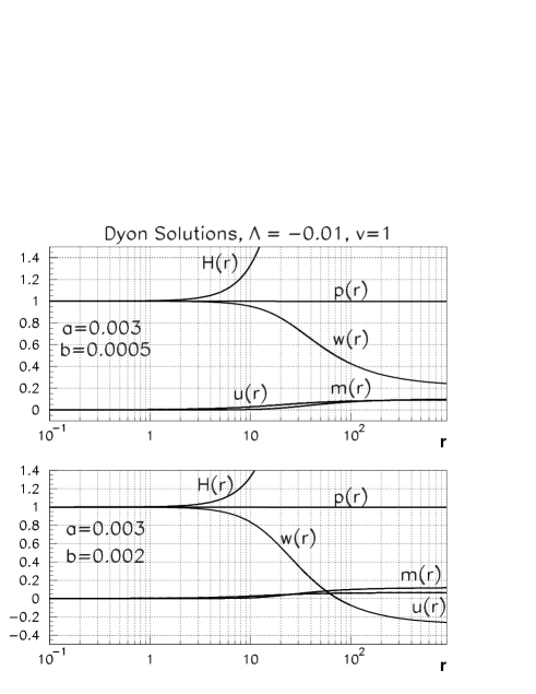
Figure 2: Dyon solutions for $\Lambda=-0.01$ and $v=1$. In the top figure $w(r)$ has no node ($n=0$), whereas in the bottom figure it has one node ($n=1$).

(c) Critical solutions

As the parameter $b$ is increased, the minimum of $H(r)$ hits zero from above, i.e. $H(r_{h})=H^{\prime}(r_{h})=0$. This constitutes a special case and needs careful examination. Numerical studies indicate that this happens in a finite range of the parameter $a$. The critical solution exists for both $u(r)=0$ and $u(r)\not=0$ cases. One example of solutions near the critical value [$(a,b)=(0.01,0.69)$] is displayed in fig. 3. $H(r)$ becomes very close to zero at $r\sim 1$. It has $(Q_{E},Q_{M},M)\sim(0.015,0.998,0.995)$.

When $b=b_{c}$, $w$ and $p$ vanish at $r=r_{h}$ as well. As $p(r_{h})=0$, $p(r)=0$ for $r\geq r_{h}$. The space ends at $r=r_{h}$. There is universality at the critical point.

Figure 3: Dyon solution for $\Lambda=-0.01$, $v=1$, $a=0.01$ and $b=0.69$. At $a=0.01$, the critical value is $b_{c}=0.7104$. $H$ almost hits the axis around $r=1$. At $b_{c}$, $p(r)=0$ for $r\geq r_{h}$. The space ends at $r_{h}$.

The numerical integration of the differential equations indicates that $m(r)$ and $u(r)$ are regular at $r=r_{h}$. The appropriate ansatz for the critical solutions with $H(r_{h})=H^{\prime}(r_{h})=0$ is, for $y=r_{h}-r\geq 0$,

$$u = u_{0}+u_{1}y+u_{2}y^{2}+\cdots$$ (76)

$$w = y^{\alpha}\Big{\{}w_{0}+w_{1}y+w_{2}y^{2}+\cdots\Big{\}}$$ (77)

$$p = y^{\beta}\Big{\{}p_{0}+p_{1}y+p_{2}y^{2}+\cdots\Big{\}}$$ (78)

$$H = y^{\gamma}\Big{\{}h_{0}+h_{1}y+h_{2}y^{2}+\cdots\Big{\}}$$ (79)

$$m = m_{0}+m_{1}y+m_{2}y^{2}+\cdots$$ (80)

Eq. (51) implies that $\gamma=2$. When $u(r)\not=0$, Eq. (52) leads to $\alpha=\hbox{${1\over 2}$}$. When $u(r)=0$, Eq. (53), instead, implies that $\alpha=\hbox{${1\over 2}$}$. Other relations obtained from eqs. (51) - (54) are

$$\Big{(}\beta-{3\over 2}\Big{)}h_{0} = {2\over r_{h}^{2}}$$ (81)

$$\beta r_{h}^{2}u_{1} = {2w_{0}^{2}u_{0}\over h_{0}}$$ (82)

$$\beta = {vw_{0}^{2}\over 2r_{h}}$$ (83)

$$m_{1} = -{v\over 2r_{h}^{2}}~{}~{}~{}.$$ (84)

The value of the index $\beta$ is unconstrained when $u=0$. However, if $u\not=0$, the consistency of eq. (51), for instance, demands that $2\beta$ be an integer. The smallest value for $\beta$ which satisfies the first relation in (84) is $\beta=2$, as $h_{0}>0$. We have confirmed this by numerical studies. The relation (46) further implies that

$${2m_{0}\over r_{h}} = 1-{\Lambda\over 3}r_{h}^{2}$$ (85)

$$m_{1} = {1\over 2}(\Lambda r_{h}^{2}-1)~{}.$$ (86)

From the two relations for $m_{1}$, one in (84) and the other in (86), $r_{h}$ is determined as a function of $v$ and $\Lambda<0$:

$$r_{h}^{2}={1\over 2|\Lambda|}\left(\sqrt{1+4v|\Lambda|}-1\right)~{}~{}.$$ (87)

To summarize, the indices in (80) are given by

$$\alpha={1\over 2}~{}~{},~{}~{}\beta=\gamma=2~{}~{}.$$ (88)

The coefficients $m_{0}$, $m_{1}$, and

$$w_{0}^{2}={4r_{h}\over v}~{}~{},~{}~{}h_{0}={4\over r_{h}^{2}}$$ (89)

are all determined by $v$ and $\Lambda$ only. We are observing the universality in the behavior of the critical solutions. The coefficients $u_{0}$ and $p_{0}$ depend on $a$ or $b$ as well.

For small $v|\Lambda|\ll 1$

$$r_{h}\sim\sqrt{v}~{}~{},~{}~{}m_{0}\sim{1\over 2}\sqrt{v}~{}~{},~{}~{}m_{1}\sim-{1\over 2}$$ (90)

$$w_{0}\sim{2\over v^{1/4}}~{}~{},~{}~{}h_{0}\sim{4\over v}$$ (91)

They are all determined by $v$ only. This universal behavior is clearly seen in the solution in fig. 3 which is very close to the critical one.

The meaning of the critical spacetime is yet to be clarified. The space ends at $r=r_{h}$. It defines a spacetime with a boundary.

Figure 4: Mass $M$ is plotted as a function of magnetic charge $Q_{M}$ for monopole solutions at $\Lambda=-0.01$ and $v=1$. The number of nodes, $n$, in $w(r)$ is also marked. In the lower branch $Q_{M}=1$ at $b=0.00168$.

(d) Spectrum of monopole and dyon solutions

Monopole and dyon solutions permit non-vanishing charges $Q_{M}$ and $Q_{E}$, although there are solutions where $Q_{M}=0$ and $Q_{E}\neq 0$ or where $Q_{E}=0$ but $Q_{M}\neq 0$. Non-zero charges $Q_{M}$ or $Q_{E}$ ensures that $Q_{\rm eff}\neq 0$ (see Eq. (64) ) so that solutions are asymptotically of the AdS Reissner-Nordström type.

In fig. 4 the mass $M$ is plotted as a function of $Q_{M}$ for monopole solutions at $\Lambda=-0.01$ and $v=1$. The behavior of the solutions near t$b=b_{c}=0.7104$ needs more careful analysis.

Figure 5: Magnetic charge $Q_{M}$ of dyon solutions as a function of the parameter $b$ is plotted with various values of the parameter $a$. At $b\sim 0.0061$, $Q_{M}$ is independent of $a$, taking the quantized value $-(4\pi)^{-1/2}=-0.2821$ within numerical errors.

Dyon solutions are found in a good portion of the $Q_{E}$-$Q_{M}$ plane. There are solutions with $Q_{M}=0$ but $Q_{E}\not=0$. Although $Q_{M}=0$, i.e. $w(\infty)=\pm 1$, $w(r)\not=0$. In the shooting parameter space $(a,b)$, these solutions correspond not exactly, but almost to a universal value for $b\sim 0.0054$. See fig. 5. More surprising is the fact that $Q_{M}$ takes a quantized value $-(4\pi)^{-1/2}$ at $b=0.0061$ independent of the value of $a$ within numerical errors. We have not understood why it should be so.

Solutions with no node in $w(r)$ have special importance, as they are stable against small fluctuations. (See section 8.) In fig. 6 the spectrum of nodeless dyon solutions are presented in the parameter space $(a,b)$. Notice that $a$ must be small enough ($a<0.005$) even for $b<0$.

Figure 6: Spectrum of nodeless dyons.

(e) Dependence of the coupling $v$ on the solutions

The ADM mass $M$ depends on the value of the coupling $v=4\pi G/e^{2}$. As shown in fig. 7, $M$ increases as $v$ gets larger and decreases when $v$ gets smaller. With fixed $(a,b)$, roughly $M\propto v$. The Yang-Mills fields $u$ and $w$ are roughly independent of $v$.

Figure 7: A typical solution showing the dependence of $v$ on the mass $m(r)$. $\Lambda=-0.01$, $a=0.003$ and $b=0.001$. $w(r)$ and $u(r)$ do not have much dependence on $v$.

6 Black hole solutions

Not long after the BK solutions were discovered, black hole solutions were also found to be contained in the EYM equations[4] if different boundary conditions were used. These solutions generated a large amount of further study, as they apparently violate the no-hair conjecture [6]. Later, EYM black holes were studied in a cosmological context by including a positive cosmological constant[10]. These black hole solutions share most of the properties as the soliton solutions, including their instability.

Recently, purely magnetic black hole solutions were found in asymptotically anti-de Sitter space [13]. These solutions are drastically different from their asymptotically Minkowski or de Sitter counterparts. There are a continuum of solutions in terms of the adjustable shooting parameter that specifies the initial conditions at the horizon. Furthermore, there exist solutions that have no node in $w$ and are in turn stable against spherically symmetric linear perturbations. Here, we discuss the solutions found by Winstanley [13] and also present new dyon black hole solutions. We also discuss the apparent shrinking of the moduli space when the magnitude of $\Lambda$ is decreased. Similar to the particle-like solutions already discussed, the moduli space becomes discrete in the $\Lambda\rightarrow 0$ limit.

6.1 Boundary conditions at the horizon

Black hole solutions are obtained numerically by specifying the boundary conditions at the horizon and shooting for regular solutions $w$, $u$, $m$ and $p$ for $r_{h}\leq r<\infty$. The location of the horizon, $r_{h}$, and the value $p(r_{h})>0$ can be arbitrarily chosen by scaling of $t$ and $r$. We look for solutions in which $H(r)>0$ for $r>r_{h}$. As $H(r_{h})=0$ but $p(r_{h})\not=0$, Eqs. (51) - (54) require that either $u$ or $w$ vanishes at the horizon. A stronger condition is obtained from the sum rule (67) with $r_{1}=r_{h}$ and $r_{2}=\infty$. Its l.h.s.  is finite so that $u(r_{h})=0$ on its r.h.s. Hence we are led to the expansion

$$w = w_{0}+w_{1}x+\cdots$$ (92)

$$u = u_{1}x+\cdots$$ (93)

$$p = 1+p_{1}x+\cdots$$ (94)

$$H = h_{1}x+\cdots$$ (95)

$$m = m_{0}+m_{1}x+\cdots$$ (96)

where $x=r-r_{h}$. We have chosen $p(r_{h})=1$ without loss of generality.

There are two adjustable shooting parameters, $(a,b)=(u_{1},w_{0})$. After inserting the ansatz into eq.’s (46) to (54) we find

$$m_{0} = \frac{r_{h}}{2}-\frac{\Lambda r_{h}^{3}}{6}$$ (97)

$$m_{1} = {v\over 2}\Bigg{\{}{(1-w_{0}^{2})^{2}\over r_{h}^{2}}+u_{1}^{2}\Bigg{\}}$$ (98)

$$h_{1} = \frac{1}{r_{h}}(1-\Lambda r_{h}^{2}-2m_{1})$$ (99)

$$w_{1} = -\frac{w_{0}(1-w_{0}^{2})}{r_{h}^{2}h_{1}}$$ (100)

$$p_{1} = -\frac{2v}{r_{h}}\Bigg{\{}(w_{1})^{2}+\frac{w_{0}^{2}u_{1}^{2}}{h_{1}^{2}}\Bigg{\}}$$ (101)

$$u_{2} = -\Bigg{\{}{w_{0}^{2}\over r_{h}^{2}h_{1}}+{1\over r_{h}}+{p_{1}\over 2}\Bigg{\}}~{}~{}.$$ (102)

The asymptotic expansion at large $r$ is the same as in (59). The ADM mass is given by $M=m(\infty)$.

6.2 New electrically and magnetically charged black hole solutions

Just as the soliton solutions, purely magnetically charged black hole solutions are obtained by setting the adjustable parameter $a$ to zero. The behavior of the solutions are similar to that of the solitons (see Ref. [13] for more information). The number of nodes $n$ in $w$ can be 0, 1, 2, $\cdots$. The black hole monopole spectrum of mass versus charge is displayed in fig. 8. It shows the spectrum for the $n=0$ and $n=1$ arms.

Figure 8: Black hole mass vs. magnetic charge $Q_{M}$ for the $n=0$ and $n=1$ arms and for different values of $\Lambda$.

Figure 9: Typical dyon black hole solutions with no node and one node. $H(r)$ and $p(r)$ were not plotted for the sake of clarity. The top figure corresponds to $(a,b)=(0.004,0.99998)$, whereas the bottom to $(0.01,0.9998)$.

Solutions with both magnetic and electric charge are obtained by giving $a$ a finite value. Dyon black hole solutions are similar to the monopole solutions except that $u$ is nonzero. At the horizon $u$ starts at zero and monotonically increases asymptotically to a finite value. $H$ starts at one and quickly diverges. $p$ starts at one and remains almost constant. Typical black hole dyon solutions are shown in Fig. 9.

Again black hole dyon solutions with no node in $w(r)$ are stable against small spherically symmetric perturbations. The spectrum of those nodeless black hole dyons in the parameter space $(a,b)$ is plotted in fig. 10. Notice the similarity between fig. 6 and fig. 10. The nodeless solutions exist only for small $a=u_{1}<0.0055$. $b=w_{0}$ must be around 1.

Figure 10: Spectrum of black hole solutions.

7 Dependence on $\Lambda$ – fractal structure

The soliton and black hole solutions depend non-trivially on the value of the cosmological constant $\Lambda$. It has not been well understood why the continuum of solutions for negative $\Lambda$ become a discrete set of solutions in the $\Lambda\rightarrow 0$ limit, and remain discrete for all $\Lambda>0$. Just as fig. 8 shows for the black hole solutions, fig. 4 and fig. 11 shows the spectrum in mass vs. magnetic charge $Q_{M}$ plane for a give $\Lambda$. The width of each branch for a given $\Lambda$ gets smaller as $\Lambda$ approaches zero. Fig. 11 indicates that as $\Lambda\rightarrow 0$, the branches collapse to one point, the BK solution, as the continuum of solutions vanishes. It is still unknown mathematically why and how this occurs.

Figure 11: The appearance and collapse of soliton solutions in $\Lambda\rightarrow 0$. The bottom figure is the blow-up of a part of the top figure near $(Q_{M},M)=(0,1)$, in which the first four Bartnik-McKinnon solutions are also marked. It is seen that as $\Lambda\rightarrow 0$, solutions on a branch collapse to a point. New branches emerge as $|\Lambda|$ becomes smaller, too.

We would like to point out that there is a fractal structure in the moduli space of the solutions. This is most clearly seen in the parameter $b$ v.s. mass $M$ plot as displayed in fig. 12. As $\Lambda$ becomes smaller, a new branch appears. The shape of branches has approximate self-similarity. Similarly, in fig. 13 the magnetic charge $Q_{M}$ is plotted against $b$. Delicate structure is observed near the critical $b=b_{c}$ which signifies the critical solution discussed in Section 5.3 (c). There may be some connection between the limiting point in the monopole spectrum and the critical solution.

Figure 12: The monopole spectrum. $b$ v.s. $M$ (mass) is plotted with various values of $\Lambda$.

Figure 13: The monopole spectrum. $b$ v.s. $Q_{M}$ (magnetic charge) is plotted with various values of $\Lambda$.

8 Stability

It has been shown that the soliton and black hole solutions in asymptotically Minkowski and de Sitter space, which necessarily have at least one node in $w(r)$, are unstable [2][11][10][3]. In contrast, the monopole and black hole solutions in the asymptotically anti-de Sitter space with no node in $w(r)$ are stable for $u=0$. One expects the presence of the electric field not to change the stability of the solitons and black hole configurations.

In this section we give a detailed discussion for establishing the stability. We shall find that in asymptotically anti-de Sitter space the boundary condition for the resultant Schrödinger problem becomes subtle, and that the previous argument given in asymptotically Minkowski space needs elaboration.

8.1 Perturbation equations

We consider small time-dependent perturbations to the static solutions to the coupled EYM equations. In the static solutions $\nu(r)=\tilde{w}(r)=0$. In the general ansatz, (18) and (28) we set

$$u(r,t) = u(r)+\delta u(r,t)$$ (103)

$$w(r,t) = w(r)+\delta w(r,t)$$ (104)

$$\tilde{w}(r,t) = \delta\tilde{w}(r,t)$$ (105)

$$\nu(r,t) = \delta\nu(r,t)$$ (106)

$$p(r,t) = p(r)+\delta p(r,t)$$ (107)

$$H(r,t) = H(r)+\delta H(r,t)$$ (108)

and $m(r,t)=m(r)+\delta m(r,t)$. Substituting (108) into the Yang-Mills equation (34) and retaining only terms linear in perturbations, one finds

$$\hskip-42.67912pt\Big{[}r^{2}u^{\prime}\delta p+r^{2}p(\delta u^{\prime}-\delta\dot{\nu})\Big{]}^{\prime}-{2uw^{2}p\over H}\bigg{(}{\delta p\over p}-{\delta H\over H}\bigg{)}-{2pw\over H}(w\delta u+2u\delta w+\delta\dot{\tilde{w}})=0$$ (109)

$$\hskip-42.67912ptr^{2}p(\delta\dot{u}^{\prime}-\delta\ddot{\nu})+r^{2}u^{\prime}\delta\dot{p}-\frac{2H}{p}\left[w\delta\tilde{w}^{\prime}-w^{\prime}\delta\tilde{w}+w^{2}\delta\nu\right]=0$$ (110)

$$\hskip-42.67912pt\Bigg{[}{w^{\prime}H\over p}\bigg{(}{\delta H\over H}-{\delta p\over p}\bigg{)}+{H\over p}\delta w^{\prime}\Bigg{]}^{\prime}+{pu\over H}(u\delta w+2w\delta u+2\delta\dot{\tilde{w}})-{p\over H}\,\delta\ddot{w}$$ (111)

$$\hskip 56.9055pt+{wu^{2}p\over H}\bigg{(}{\delta p\over p}-{\delta H\over H}\bigg{)}-\frac{w(1-w^{2})}{r^{2}p^{2}}\delta p+{1-3w^{2}\over r^{2}p}\delta w=0$$ (112)

$$\hskip-42.67912pt\Bigg{[}{H\over p}(\delta\tilde{w}^{\prime}+w\delta\nu)\Bigg{]}^{\prime}+{p\over H}(u^{2}\delta\tilde{w}-2u\delta\dot{w}-w\delta\dot{u}-\delta\ddot{\tilde{w}})$$ (113)

$$\hskip 56.9055pt-{uwp\over H}\bigg{(}{\delta\dot{p}\over p}-{\delta\dot{H}\over H}\bigg{)}+\frac{(1-w^{2})}{r^{2}p}\delta\tilde{w}+\frac{H}{p}w^{\prime}\delta\nu=0~{}~{}.$$ (114)

The Einstein equations (45) and (47) yield

$$\hskip-42.67912pt\delta m^{\prime}=v\Bigg{\{}r^{2}p^{2}u^{\prime}(\delta u^{\prime}-\delta\dot{\nu})+\Big{(}r^{2}u^{\prime 2}+{2u^{2}w^{2}\over H}\Big{)}p\delta p+\Big{(}w^{\prime 2}-\frac{p^{2}u^{2}w^{2}}{H^{2}}\Big{)}\delta H$$ (115)

$$\hskip 42.67912pt+2Hw^{\prime}\delta w^{\prime}+\frac{2uwp^{2}}{H}(w\delta u+u\delta w+\delta\dot{\tilde{w}})-\frac{2w(1-w^{2})}{r^{2}}\delta w\Bigg{\}}$$ (116)

$$\hskip-42.67912pt\Bigg{(}{\delta p\over p}\Bigg{)}^{\prime}=-{4v\over r}\Bigg{\{}w^{\prime}\delta w^{\prime}+{p^{2}u^{2}w^{2}\over H^{2}}\bigg{(}{\delta p\over p}-{\delta H\over H}\bigg{)}+{p^{2}uw\over H^{2}}(w\delta u+u\delta w+\delta\dot{\tilde{w}})\Bigg{\}}$$ (117)

$$\hskip-42.67912pt\delta\dot{H}=-{4vH\over r}\Big{\{}w^{\prime}\delta\dot{w}-u(w^{\prime}\delta\tilde{w}-w\delta\tilde{w}^{\prime})+uw^{2}\delta\nu\Big{\}}~{}~{}.$$ (118)

There is residual gauge invariance specified by a gauge function $\Omega(r,t)$ in (12) and (22). Making use of this freedom, one can always set either $\delta u(r,t)=0$ or $\delta\nu(r,t)=0$.

8.2 Stability analysis

In examining time-dependent fluctuations around monopole solutions for which $u(r)=0$, it is convenient to work in the $\delta u(t,r)=0$ gauge. Eqs. (109), (110), and (114) become

$$\hskip-28.45274pt(r^{2}p\delta\nu)^{\prime}=-{2pw\over H}\,\delta\tilde{w}$$ (119)

$$\hskip-28.45274ptr^{2}p\delta\ddot{\nu}+{2H\over p}(w\delta\tilde{w}^{\prime}-w^{\prime}\delta\tilde{w}+w^{2}\delta\nu)=0$$ (120)

$$\hskip-28.45274pt\bigg{[}{H\over p}(\delta\tilde{w}^{\prime}+w\delta\nu)\bigg{]}^{\prime}-{p\over H}\,\delta\ddot{\tilde{w}}+{1-w^{2}\over r^{2}p}\,\delta\tilde{w}+{H\over p}\,w^{\prime}\delta\nu=0~{}~{},$$ (121)

whereas Eqs. (112), (116), (117), and (118) become

$$\hskip-28.45274pt\Bigg{[}{H\over p}\Bigg{\{}w^{\prime}\bigg{(}{\delta H\over H}-{\delta p\over p}\bigg{)}+\delta w^{\prime}\Bigg{\}}\Bigg{]}^{\prime}-{p\over H}\,\delta\ddot{w}-{w(1-w^{2})\over r^{2}p^{2}}\,\delta p+{1-3w^{2}\over r^{2}p}\,\delta w=0$$ (122)

$$\hskip-28.45274pt\delta m^{\prime}=v\Bigg{\{}w^{\prime 2}\delta H+2Hw^{\prime}\delta w^{\prime}-{2w(1-w^{2})\over r^{2}}\,\delta w\Bigg{\}}$$ (123)

$$\hskip-28.45274pt\bigg{(}{\delta p\over p}\bigg{)}^{\prime}=-{4v\over r}\,w^{\prime}\delta w^{\prime}$$ (124)

$$\hskip-28.45274pt\delta H=-{4v\over r}\,Hw^{\prime}\delta w~{}~{}.$$ (125)

Notice that Eqs. (119) - (121) involve only $\delta\nu$ and $\delta\tilde{w}$, defining the odd parity group, whereas Eqs. (122) - (125) involve only $\delta w$, $\delta H$, and $\delta p$, defining the even parity group. The number of the equations is larger than the number of the unknown functions. Indeed, one equation in each group follows from the others.

To derive the equation for each unknown function in a closed form, we introduce the tortoise radial coordinate $\rho$ by

$${d\rho\over dr}={p\over H}$$ (126)

with which the equations for $w$, $p$, and $m$ become

$${d^{2}w\over d\rho^{2}} = -{H\over r^{2}p^{2}}\,w(1-w^{2})$$ (127)

$${dp\over d\rho}~{} = -{2vp^{2}\over rH}\bigg{(}{dw\over d\rho}\bigg{)}^{2}$$ (128)

$${dm\over d\rho} = v\Bigg{\{}p\bigg{(}{dw\over d\rho}\bigg{)}^{2}+{H\over 2r^{2}p}\,(1-w^{2})^{2}\Bigg{\}}~{}~{}.$$ (129)

The range of $\rho$ is finite, $0\leq\rho\leq\rho_{\rm max}$, since $p\rightarrow p_{0}$ and $H\rightarrow|\Lambda|r^{2}/3$ as $r\rightarrow\infty$:

$$\rho=\cases{r&for $r\sim 0$\cr\kern 8.0pt\cr\rho_{\rm max}-{\displaystyle 3p_{0}\over\displaystyle|\Lambda|r}&for $r\sim\infty$\cr}$$ (130)

where $p=p_{0}+{\rm O}(1/r)$.

In the odd parity group Eq. (119) expresses $\delta w$ in terms of $\delta\nu$. Substituting it into Eq. (120) and making use of (127), one finds

$$\hskip-28.45274pt\Bigg{\{}-{d^{2}\over d\rho^{2}}+U_{\beta}(\rho)\Bigg{\}}\beta=\omega^{2}\beta$$ (131)

$$\hskip-28.45274ptU_{\beta}=\frac{H}{r^{2}p^{2}}(1+w^{2})+\frac{2}{w^{2}}\left(\frac{dw}{d\rho}\right)^{2}~{}~{},$$ (132)

$$\hskip-28.45274pt\delta\nu={w\over r^{2}p}\,\beta~{}~{}~{},~{}~{}~{}\delta\tilde{w}=-{1\over 2w}\,{d\over d\rho}(w\beta)~{}~{}.$$ (133)

Here we have supposed fluctuations to be harmonic: $\delta\nu(r,t)=e^{-i\omega t}\delta\nu(\rho)$ and $\delta\tilde{w}(r,t)=e^{-i\omega t}\delta\tilde{w}(\rho)$. Eq. (121) follows from (119), (120), and (127).

In the even parity group, (124) and (125) express $\delta p$ and $\delta H$ ($\delta m$) in terms of $\delta w$. Eq. (123) automatically follows from (124), (125), (127) and (128). Eq. (122) becomes, with the use of (124), (125) and (127),

$$\hskip-28.45274pt\Bigg{\{}-{d^{2}\over d\rho^{2}}+U_{w}(\rho)\Bigg{\}}\delta w=\omega^{2}\delta w~{}~{},$$ (134)

$$\hskip-28.45274ptU_{w}=\frac{H}{r^{2}p^{2}}\,(3w^{2}-1)+4v\frac{d}{d\rho}\bigg{[}\frac{p}{rH}\Bigg{(}{dw\over d\rho}\bigg{)}^{2}\Bigg{]}$$ (135)

Again harmonic fluctuations $\delta w(r,t)=e^{-i\omega t}\delta w(\rho)$ are supposed.

Eqs. (133) and (135) have the same form as the Schrödinger equation on a one-dimensional interval. Both of the potentials $U_{\beta}$ and $U_{w}$ are singular at $\rho=0$, behaving as $+2/\rho^{2}$. $U_{\beta}$ has an additional singularity if $w$ has a zero at $\rho_{k}$; $U_{\beta}\sim+2/(\rho-\rho_{k})^{2}$.

The integrated energy-momentum density $T^{ab}\sqrt{-g}\,d^{3}x$ due to fluctuations must remain finite. At the origin $r=0$ it implies that $\delta w=\delta\tilde{w}=0$ whereas $\delta\nu={\rm O}(1)$. Taking advantage of the general coordinate invariance, one can impose $\delta p=0$ and $\delta H=-2\delta m/r=0$. At $r\sim\infty$, $\delta w^{\prime},\delta\tilde{w}^{\prime},\delta\nu={\rm O}(r^{-2})$. These are mild boundary conditions. One can impose more strict conditions such as the regularity at $r=0$ and vanishing at $r=\infty$. As physical perturbations we demand that all $\delta w$, $\delta\tilde{w}$, $\delta\nu$, $\delta H$, and $\delta p$ vanish at $r=\infty$.

In Eq. (133) the potential $U_{\beta}(\rho)$ is positive definite. However, this does not necessarily mean that the eigenvalue $\omega^{2}$ is positive definite. It depends on the boundary condition. Clearly $\beta(0)=0$. At $\rho=\rho_{\rm max}$, $\delta\nu=\delta\tilde{w}=0$ so that $\beta^{\prime}+h\beta=0$ where $h=w^{\prime}/w$. Note that

$$h={1\over w}{dw\over d\rho}\Bigg{|}_{\rho_{\rm max}}={|\Lambda|\over 3p_{0}}\,{r^{2}\over w}{dw\over dr}\Bigg{|}_{r=\infty}={|\Lambda|w_{1}\over 3p_{0}w_{0}}$$ (136)

where $w_{j}$’s are defined in (59). For the monopole configurations with no nodes in $w$, $h<0$ ($h>0$) when $w$ is monotonically decreasing (increasing).

Following Courant and Hilbert [28], we define

$$\hskip-28.45274pt{\cal D}(\varphi;h)=\int_{0}^{\rho_{\rm max}}d\rho\,\Big{\{}\varphi^{\prime}(\rho)^{2}+U_{\beta}(\rho)\,\varphi(\rho)^{2}\Big{\}}+h~{}\varphi(\rho_{\rm max})^{2}$$ (137)

$$\hskip-28.45274pt{\cal N}(\varphi)=\int_{0}^{\rho_{\rm max}}d\rho\,\varphi(\rho)^{2}~{}~{}.$$ (138)

If $w(r)$ is nodeless, then $U_{\beta}(\rho)$ is regular on the interval except at $\rho=0$. The equation implies that $\beta={\rm O}(\rho^{2})$ near the origin. In this case, for an eigenfunction $\beta(\rho)$ in (133) satisfies

$$\omega^{2}={{\cal D}(\beta)\over{\cal N}(\beta)}~{}~{}.$$ (139)

It follows immediately that all eigenvalues $\omega^{2}$ are positive definite if $h\geq 0$ so that the solution is stable against small odd-parity perturbations.

For $h<0$ more careful analysis is necessary. The lowest eigenvalue $\omega^{2}\equiv\lambda_{1}$ in the eigenvalue equation (133) is exactly the lower bound of the set of values assumed by the functional ${\cal D}(\varphi,h)$, where $\varphi$ is any function continuous on the interval $[0,\rho_{\rm max}]$ with piecewise continuous derivatives satisfying $\varphi(0)=1$ and ${\cal N}(\varphi)=1$.

$$\lambda_{1}(h)={\rm min}_{\varphi}~{}{\cal D}(\varphi;h)~{}~{}.$$ (140)

If $\lambda_{1}>0$, then the solution is stable against odd-parity perturbations. Suppose that $\varphi_{1}(\rho)$ saturates the lower bound for $h_{1}$: $\lambda_{1}(h_{1})={\cal D}(\varphi_{1};h_{1})$. As

$$\lambda_{1}(h_{1}) = {\cal D}(\varphi_{1};h_{2})+(h_{1}-h_{2})\varphi_{1}(\rho_{\rm max})^{2}$$ (141)

$$\geq \lambda_{1}(h_{2})+(h_{1}-h_{2})\varphi_{1}(\rho_{\rm max})^{2}~{},$$ (142)

$\lambda_{1}(h)$ is a monotonically increasing function of $h$. Hence, if $\lambda_{1}(h_{1})>0$, then $\lambda_{1}(h)>0$ for $h\geq h_{1}$.

To establish the stability we utilize the residual gauge invariance. There is a zero-mode (with $\omega^{2}=0$) for Eq.  (133) with an appropriate boundary condition $h_{0}$. In the $\Lambda=0$ case the existence of the zero-mode was utilized to prove the instability of the BK and black hole solutions which has at least one node in $w(r)$ [26][27]. Consider the time-independent gauge function $\Omega(r)$ in (12). For $|\Omega|\ll 1$, $\delta\nu=d\Omega/dr$ and $\delta\tilde{w}=-w\Omega$. Eq. (119) is satisfied if

$${d\over d\rho}\bigg{(}{r^{2}p^{2}\over H}{d\Omega\over d\rho}\bigg{)}=2w^{2}\Omega~{}~{}.$$ (143)

As $\Omega(0)=0$, $\Omega\sim a\rho+{\rm O}(\rho^{3})$ for $\rho\sim 0$. Hence Eq. (143) determines $\Omega(r)$ up to an over-all constant. $\beta_{0}=(r^{2}p^{2}/wH)(d\Omega/d\rho)$ is the zero mode of Eq. (133) and $U_{\beta}=\beta_{0}^{\prime\prime}/\beta_{0}$, where $\Omega^{\prime}\equiv d\Omega/d\rho$ etc. In this case $\Omega(\rho_{\rm max})\not=0$ and $h_{0}=-\beta_{0}^{\prime}/\beta_{0}|_{\rho_{\rm max}}$ differs from $h$ in the eigenvalue problem under consideration. If $h>h_{0}$, then $\lambda_{1}(h)>0$, establishing the stability. As $d(w\beta_{0})/d\rho=2w^{2}\Omega$,

$$h=h_{0}+{2w^{2}H\Omega\over r^{2}p^{2}\Omega^{\prime}}~{}~{}.$$ (144)

Nodeless solutions ($w>0$) are stable if $\Omega/\Omega^{\prime}>0$ at $\rho_{\rm max}$.

Solving (143) numerically, we have determined $\Omega(\rho)$ to find that indeed $h>h_{0}$ for nodeless solutions. This analysis also shows that $h$ becomes exactly $h_{0}$ for the configuration with $w(r=\infty)=0$. In this limiting case the zero mode is not normalizable; it diverges as $(\rho-\rho_{\rm max})^{-1}$.

This is a general behavior. When $w$ has a node at $\rho_{k}<\rho_{\rm max}$, there appears a negative $\omega^{2}$ mode which behaves as $(\rho-\rho_{k})^{-1}$ near $\rho_{k}$.

If $w(r)$ has $n$ nodes, i.e. $w(r_{j})=0$ ($j=1,\cdots,n$), the potential $U_{\beta}$ develops $(\rho-\rho_{j})^{-2}$ singularities. Volkov et al. have shown for the BK solutions in the $\Lambda=0$ case that there appear exactly $n$ negative eigenmodes ($\omega^{2}<0$) if $w$ has $n$ nodes [26]. A similar conclusion has been obtained for black hole solutions as well [27]. Their argument needs elaboration in the $\Lambda<0$ case, however.

To investigate the eigenvalue spectrum of (133) in this case, it is convenient to consider the dual equation as was done in [26]. One can write the Schrödinger equation in (133) as

$$\hskip-28.45274ptQ_{+}Q_{-}\varphi_{n}=\lambda_{n}\varphi_{n}$$ (145)

$$\hskip-28.45274ptQ_{\pm}=\pm{d\over d\rho}+{\beta_{0}^{\prime}\over\beta_{0}}$$ (146)

where $\beta_{0}(\rho)$ is the zero mode described above. $\varphi_{n}={\rm O}(\rho^{2})$ near $\rho=0$ and $\varphi_{n}^{\prime}+h\varphi_{n}=0$ at $\rho_{\rm max}$. The dual equation is given by

$$\hskip-28.45274ptQ_{-}Q_{+}\tilde{\varphi}_{n}=\bigg{\{}-{d^{2}\over d\rho^{2}}+\tilde{U}_{\beta}\bigg{\}}\tilde{\varphi}_{n}=\lambda_{n}\tilde{\varphi}_{n}$$ (147)

$$\hskip-28.45274pt\tilde{U}_{\beta}=-{H\over r^{2}p^{2}}(1+w^{2})-{8ww^{\prime}H\Omega\over r^{2}p^{2}\Omega^{\prime}}+8\bigg{(}{w^{2}H\Omega\over r^{2}p^{2}\Omega^{\prime}}\bigg{)}^{2}~{}~{}.$$ (148)

$\varphi_{n}$ and $\tilde{\varphi}_{n}$ are related to each other by

$$\tilde{\varphi}_{n}=\cases{Q_{-}\varphi_{n}&for $\lambda_{n}\not=0$\cr{\varphi_{n}}^{-1}={\beta_{0}}^{-1}&for $\lambda_{n}=0$\cr}$$ (149)

However, the boundary condition for $\tilde{\varphi}_{n}(\rho)$ depends on $\lambda_{n}$:

$$\hskip-28.45274pt\tilde{\varphi}_{n}(0)=0$$ (150)

$$\hskip-28.45274pt\tilde{\varphi}_{n}^{\prime}(\rho_{\rm max})+\tilde{h}_{n}\tilde{\varphi}_{n}(\rho_{\rm max})=0$$ (151)

$$\hskip-28.45274pt\tilde{h}_{n}=-h_{0}-{\lambda_{n}\over h-h_{0}}~{}~{}.$$ (152)

Figure 14: Eigenvalues $\lambda_{n}$ ($n=1,2,3$) in the dual Schrödinger equation (148) with the boundary condition (152) are displayed for monopole configurations with varying value of $b$. $\Lambda=-0.01$ and $v=1$. When $w(\infty)$ develops a node, the negative eigenvalue mode arises, signaling the instability of the solution. $w(\infty)=0$ at $b=0.00168$, where the numerical evaluation of $\lambda_{1}$ becomes difficult.

The advantage of considering the dual equation is that the dual potential $\tilde{U}_{\beta}(\rho)$ is regular except at $\rho=0$ where it behaves as $+6/\rho^{2}$. However, the eigenvalue $\lambda_{n}$ has to be determined self-consistently such that the boundary condition (152) is satisfied. We have determined $\lambda_{n}$’s numerically for the monopole configurations in the lower branch in fig. 4. The first, second and third eigenvalues are displayed in fig. 14. One sees that $\lambda_{1}>0$ for the nodeless configurations, but the unstable mode develops when $w$ has a node.

The wave function of the unstable mode in the original equation, not in the dual equation, diverges at the zeroes of $w(r)$. In other words, the instability sets in around the zeroes of $w(r)$. The potential $U_{\beta}(\rho)$ and $\tilde{U}_{\beta}(\rho)$ for the solution at $b=0.0025$ are plotted in fig. 15. At the node of $w$, $U_{\beta}$ diverges, but $\tilde{U}_{\beta}$ remains finite. The wave function $\tilde{\varphi}_{1}(\rho)$ of the lowest eigenvalue ($\lambda_{1}=-0.0033)$ and the corresponding $\varphi_{1}(\rho)$ also have been plotted in fig. 15.

Figure 15: $U_{\beta}(\rho)$ and $\tilde{U}_{\beta}(\rho)$ for the monopole solution at $b=0.0025$, $\Lambda=-0.01$, and $v=1$. The wave function of the unstable mode ($\lambda=-0.0033$) are also plotted. $\tilde{\varphi}_{1}(\rho)$ in the dual equation (148) is a regular smooth function, but $\varphi_{1}(\rho)$ in the original equation (146) diverges at the zero of $w$.

For even-parity perturbation the potential $U_{w}(\rho)$ in Eq. (135) is not positive definite. The first term in $U_{w}$ becomes negative for $w^{2}<1/3$. The second term also can become negative when $w^{\prime}$ vanishes at finite $r$. We have solved the Schrödinger equation (135) numerically for typical monopole solutions, and found that for the solutions with no node in $w(r)$, the eigenvalues $\omega^{2}$ are always positive even if $w(r=\infty)<1/\sqrt{3}$.

Hence we have established the stability of the monopole solutions with no node in $w(r)$.

9 Summary

New monopole, dyon, and black hole solutions to the Einstein-Yang-Mills equations have been found in asymptotically anti-de Sitter space. The solutions with no node in the non-Abelian field strengths are shown to be stable against spherically symmetric perturbations. The non-trivial boundary condition plays a crucial role in developing the instability for solutions with nodes. The stability of nodeless dyon solutions need to be established.

Though electric and magnetic charges of monopole and dyon solutions are not quantized in classical theory, they are expected to be quantized in quantum theory. If this is the case, then at least solutions with the smallest charge would become absolutely stable.

We have also found the critical spacetime solutions which end at finite $r$. These solutions may have connections to black hole solutions, though more detailed study is necessary.

The solutions found in the present paper may have profound consequences in the evolution of the early universe which may have gone through the anti-de Sitter phase. We hope to report on these subjects in future publications.

Acknowledgments

This work was supported in part by the U.S. Department of Energy under contracts DE-FG02-94ER-40823, DE-FG02-87ER40328 and DE-AC02-98CH10886.

References

• [1] R. Bartnik and J. McKinnon, Phys. Rev. Lett 61 , 141 (1988).
• [2] N. Straumann and Z. Zhou, Phys. Lett. B237 353 (1990); Phys. Lett. B243 33 (1990); Z. Zhou and N. Straumann, Nucl. Phys. B360, 180 (1991).
• [3] M. S. Volkov and D. Gal’tsov, (preprint) hep-th/9810070 (1998).
• [4] P. Bizon, Phys. Rev. Lett. 64 , 2844 (1990).
• [5] H. KΓΌnzle and A. Masood-ul-Alam, J. Math. Phys. 31 No. 4 928 (1990).
• [6] M. Heusler, Black Hole Uniqueness Theorems. Cambridge University Press, (1996).
• [7] P. Breitenlohner, G. Lavrelashvili and D. Maison, preprint, gr-qc/9708036 (1997).
• [8] S. Deser, Phys. Lett. B64 463 (1976).
• [9] J.A. Smoller and A. G. Wasserman, Comm. Math. Phys. 194, 707 (1998).
• [10] M.S. Volkov, N. Straumann, G. Lavrelashvili, M. Huesler and O. Brodbeck, Phys. Rev. D 54 7243 (1996); T. Torii, K. Maeda and T. Tachizawa, Phys. Rev. D 52 R4272 (1995).
• [11] B. Greene, S. Mathur, and C. O’Niell, Phys. Rev. D 47 2242 (1993); K. Lee, V. Nair and E. Weinberg, Phys. Rev. Lett. 68 , 1100 (1992).
• [12] O. Brodbeck, M. Huesler, G. Lavrelashvili, N. Straumann and M.S. Volkov, Phys. Rev. D 54 7338 (1996).
• [13] E. Winstanley, Class. Quant. Grav 16, 1963, (1999).
• [14] J. Bjoraker and Y. Hosotani, gr-qc/9906091 (1999), to appear in Phys.Β Rev.Β Lett.
• [15] Y.Β Hosotani and J.Β Bjoraker, gr-qc/9907091, in the Proceedings of the 8th Canadian Conference on β€œGeneral Relativity and Relativistic Astrophysics”, page 285 (AIP, 1999); gr-qc/0001105, β€œMonopoles and dyons in the pure Einstein-Yang-Mills theory”.
• [16] A. Ershov and D. Galt’sov, Phys. Lett. A 138 , 160 (1989); Phys. Lett. A 150 , 159 (1990).
• [17] J.Β Maldacena, Adv.Β Theoret.Β Math.Β Phys.Β 2, 231 (1998); E. Witten, Adv.Β Theoret.Β Math.Β Phys.Β 2, 253 (1998); ibid. 2, 505 (1998).
• [18] Y. Brihaye, B. Hartmann, and J. Kunz, Phys. Lett. B441 77 (1998); Y. Brihaye, B. Hartmann, J. Kunz and N. Tell, Phys. Rev. D60 10416 (1999).
• [19] A. Lugo and F. Schaposnik, Phys. Lett. B467 43 (1999); A.Β Lugo, E.F.Β Moreno and F.Β Schaposnik, hep-th/9911209.
• [20] M. Banados, C. Teitelboim, and J. Zanelli, Phys. Rev. Lett. 69 1849 (1992); M. Banados, M. Henneaux, C. Teitelboim, and J. Zanelli, Phys. Rev. D48 1506 (1993);
• [21] B.Β Tekin, hep-th/9902090; A.Β Ferstl, B.Β Tekin, and V.Β Weir, hep-th/0002019.
• [22] G. ’t Hooft, Nucl, Phys. B 79, 276 (1974); A. Polyakov, JETP Lett. 20 194 (1974).
• [23] B. Julia and A. Zee, Phys. Rev. D 11, 2227 (1975).
• [24] E. Witten, Phys. Rev. Lett. 38 121 (1977).
• [25] P. ForgΓ‘cs and N.S. Manton, Comm. Math. Phys. 72, 15 (1980).
• [26] M.S. Volkov, O. Brodbeck, G. Lavrelashvili, and N. Straumann, Phys. Lett. B349, 438 (1995); O. Brodbeck and N. Straumann, J. Math. Phys. 37, 1414 (1996).
• [27] P.Β Kanti and E.Β Winstanley, gr-qc/9910069.
• [28] R.Β Courant and D.Β Hilbert, in β€œMethods of Mathematical Physics”, Volume 1, Chapter 6, (Interscience Publishers, New York, 1953).