Abstract

The finite temperature Casimir free energy is calculated for a dielectric ball of radius $a$ embedded in an infinite medium. The condition $\epsilon\mu=1$ is assumed for the inside/outside regions. Both the Green function method and the mode summation method are considered, and found to be equivalent. For a dilute medium we find, assuming a simple ”square” dispersion relation with an abrupt cutoff at imaginary frequency $\hat{\omega}=\omega_{0}$, the high temperature Casimir free energy to be negative and proportional to $x_{0}\equiv\omega_{0}a$. Also, a physically more realistic dispersion relation involving spatial dispersion is considered, and is shown to lead to comparable results.

1 Introduction

The Casimir effect has in recent years attracted considerable interest. For reviews on this topic see, for example, Plunien et al.[1], Mostepanenko and Trunov[2], and Milton [3]. The problem has been rather difficult to solve, once curved boundaries are present, because of divergences in the formalism and insufficient contact with experiments. In this paper we will consider a compact ball of radius a, permittivity $\epsilon_{1}$ and permeability $\mu_{1}$, situated in an infinite medium whose corresponding material constants are $\epsilon_{2}$ and $\mu_{2}$.

We shall take

$$\epsilon_{1}\mu_{1}=\epsilon_{2}\mu_{2}=1$$ (1)

so that the photon velocity is everywhere equal to $c$.

The relativistic condition (1) was, in the context of the Casimir effect, to our knowledge first introduced by Brevik and Kolbenstvedt [4, 5]. The reason why this particular condition was imposed was that when calculating the Casimir surface force density on the sphere, in this paper called $f$, one avoids thereby the subtraction of a contact term: the contact term turns out to be zero just as in the case of a singular spherical conducting sphere in a vacuum [6]. Later, this kind of medium has been considered from various viewpoints [7 - 19]. A common feature of most of these papers is the use of macroscopic electrodynamics of continuous media.

The main purpose of the present paper is to consider the Casimir effect for a compact ball satisfying the condition (1), at finite temperatures. Finite temperature Casimir theory has been considered previously by several authors, e.g., Lifshitz [20], Fierz [21], Sauer [22], Mehra [23], Brown and Maclay [24], Milton et al. [25], Revzen et al. [26], and Klich [19]. Also the very recent extensive treatise of Feinberg et al. [27] ought to be mentioned, since it describes in detail the characteristic properties of the high temperature limit, and contains also an extensive reference list.

We start in the next section by considering, as a first step, the $T=0$ theory, and demonstrate the equivalence between the Green function method and the mode summation method. The equivalence has of course to hold if the theory is to make sense physically, but the equivalence is not so easy to see by a mere inspection of the mathematics. A detailed calculation is desirable. In section 3 we generalize the Casimir energy expression obtained in [15] to the fourth order in the diluteness parameter $\xi$; cf. Eq. (15) and the definition in Eq. (7). In section 4 we consider the Casimir free energy $F(T)$ at finite $T$, emphasizing the difference between $F(T)$ and the Casimir energy $E(T)$, and give an order of magnitude estimate of $F(T)$ in the case of a dilute medium endowed with a ”square” dispersion relation implying a sharp high frequence cutoff at imaginary frequency $\hat{\omega}=\omega_{0}$. The presence of a dispersion-induced strong, negative, cutoff-dependent contribution to the Casimir energy (or free energy, for finite $T$), seems first to have been pointed out by Candelas [28], for the case of a perfectly conducting shell.

At high temperatures we find $F(T)$ to be negative, decreasing linearly with $T$. This agrees with results found previously in [26] and [27]. The Casimir energy $E(T)$ itself tends to zero at high temperatures.

2 Equivalence between the Green function approach and the mode sum approach when $T=0$. Nondispersive medium

In this section we consider first the Casimir surface force density $f$ at zero temperature, for a nondispersive medium. There are in principle two different methods for calculating $f$ (more precisely, the part of $f$ that is independent of the high frequency cutoff):

The first method is to make use of the Green functions. There are two scalar Green functions, corresponding to two different electromagnetic modes. Again, this method can be carried out in one of two different ways:

1. First, one can evaluate $f$ as the difference between the radial Maxwell stress tensor components on the outside and inside of the surface $r=a$. We have to subtract off the volume terms in the scalar Green functions, so that only the boundary dependent terms are left. This regularization ensures that the surface force goes to zero when $a\to\infty$, which is as we expect on physical grounds. Also, this regularization permits us to calculate the Casimir energy $E$ once $f$ is known, by the formula $\partial E/\partial a=-4\pi a^{2}f$. (At $T=0$, $E$ is the same as the free energy $F$.)

2. Alternatively, one can calculate the energy $E$ by integrating the Maxwell energy density over the volume, retaining, as above, only the boundary dependent terms in the Green functions. The outcome of these two approaches are of course in agreement.

The Green function method was first employed by Milton, for the case of an ordinary dielectric ball [29], and was later applied to the case of an $\epsilon\mu=1$ ball in Ref. [4].

The result of the calculation can be given as follows. After a complex frequency rotation $\omega\to i\hat{\omega}$ we can express all physical quantities as integrals over frequencies $\hat{\omega}$ along the imaginary frequency axis. The cutoff dependence is omitted (it disappears in the regularization procedure). We define Riccati-Bessel functions $s_{l}$ and $e_{l}$ by ($x=\hat{k}a)$

$$s_{l}(x)=\sqrt{\frac{\pi x}{2}}I_{\nu}(x),\qquad e_{l}(x)=\sqrt{\frac{2x}{\pi}}K_{\nu}(x),$$ (2)

corresponding to the Wronskian $W\{s_{l},e_{l}\}=-1$. Here $\nu=l+\frac{1}{2}$; $I_{\nu}$ and $K_{\nu}$ are modified Bessel functions. We introduce two dispersion functions $\Delta_{l}^{\mathrm{\!TE}}$and $\Delta_{l}^{\mathrm{\!TM}}$corresponding to the TE and TM modes:

$$\Delta_{l}^{\mathrm{\!TE}}(x)=\sqrt{\epsilon_{1}\mu_{2}}s_{l}^{\prime}(x)e_{l}(x)-\sqrt{\epsilon_{2}\mu_{1}}s_{l}(x)e_{l}^{\prime}(x),$$ (3)

$$\Delta_{l}^{\mathrm{\!TM}}(x)=\sqrt{\epsilon_{2}\mu_{1}}s_{l}^{\prime}(x)e_{l}(x)-\sqrt{\epsilon_{1}\mu_{2}}s_{l}(x)e_{l}^{\prime}(x).$$ (4)

The Casimir energy as derived in [4] on the basis of the Green function can be written as

$$E=\frac{1}{2a}\frac{(\mu_{1}-\mu_{2})^{2}}{\mu_{1}\mu_{2}}\int_{-\infty}^{\infty}\frac{dy}{2\pi}\,e^{i\delta y}\sum_{l=1}^{\infty}\frac{2l+1}{4}\frac{x}{\Delta_{l}^{\mathrm{\!TE}}(x)\Delta_{l}^{\mathrm{\!TM}}(x)}\left[\lambda_{l}^{2}(x)\right]^{\prime}.$$ (5)

Here $y=\hat{\omega}a$, $x=|y|$; the time difference $\tau=t-t^{\prime}$ has been Euclidean rotated, $\tau\to i\hat{\tau}$, and $\delta=\hat{\tau}/a$ is the time-splitting parameter. Moreover, we have defined the function $\lambda_{l}(x)$ as $\lambda_{l}(x)=[s_{l}(x)e_{l}(x)]^{\prime}$ [In Ref [4] we used the symbols $D_{l}(x)$ and $\tilde{D}_{l}(x)$; the relations between these quantities and those defined by (3) and (4) are $D_{l}(x)=-\sqrt{\mu_{1}\mu_{2}}\Delta_{l}^{\mathrm{\!TE}}(x)$ and $\tilde{D}_{l}(x)=-\sqrt{\mu_{1}\mu_{2}}\Delta_{l}^{\mathrm{\!TM}}(x)$. ]

Consider next the second method, which consists in summing over the modes by means of contour integration. This method was recently used in Ref. [15], and is in turn based on the technique developed by Lambiase and Nesterenko [31] and Nesterenko and Pirozhenko [32]. One gets (when we supply the same parameter $\delta$ as above)

$$E=-\frac{1}{2a}\sum_{l=1}^{\infty}(2l+1)\int_{-\infty}^{\infty}\frac{dy}{2\pi}\,e^{i\delta y}x\frac{d}{dx}\ln\left[\Delta_{l}^{\mathrm{\!TE}}(x)\Delta_{l}^{\mathrm{\!TM}}(x)\right].$$ (6)

Introducing the parameter $\xi$ by

$$\xi=\frac{\epsilon_{1}-\epsilon_{2}}{\epsilon_{1}+\epsilon_{2}}=\frac{\mu_{2}-\mu_{1}}{\mu_{2}+\mu_{1}},$$ (7)

the expression (6) can alternatively be written as

$$E=-\frac{1}{2a}\sum_{l=1}^{\infty}(2l+1)\int_{-\infty}^{\infty}\frac{dy}{2\pi}\,e^{i\delta y}x\frac{d}{dx}\ln\left[1-\xi^{2}\lambda_{l}^{2}(x)\right].$$ (8)

The two methods thus lead to two expressions for the Casimir energy, given by Eqs. (5) and (6). The expressions, of course, have to be equal, but to see the equality is not quite trivial by mere inspection. The equality is tantamount to the equality

$$\left[\Delta_{l}^{\mathrm{\!TE}}(x)\Delta_{l}^{\mathrm{\!TM}}(x)\right]^{\prime}=-\frac{(\mu_{1}-\mu_{2})^{2}}{4\mu_{1}\mu_{2}}\left[\lambda_{l}^{2}(x)\right]^{\prime}.$$ (9)

Now it turns out that this equality is not so difficult to prove after all if we insert the expressions (3) and (4) on the left hand side and take into account the above mentioned Wronskian between $s_{l}$ and $e_{l}$. Actually, the expression (6) was also made use of in the Green-function calculation of Milton and Ng [13].

3 A remark on the dilute ball when T=0

Before leaving the zero temperature theory let us make a brief remark on the nondispersive dilute ball, meaning that

$$|\xi|\ll 1.$$ (10)

The most practical expression to make use of for the Casimir energy, is that of Eq.(8). We expand the logarithm to fourth order in $\xi$:

$$\ln(1-\xi^{2}\lambda_{l}^{2})=-\xi^{2}\lambda^{2}_{l}(x)-\frac{1}{2}\xi^{4}\lambda_{l}^{4}+{\cal O}(\xi^{6}),$$ (11)

and make the following steps:

1. put $\delta=0$;

2. perform a partial integration in Eq.(8);

3. interchange summation and integration signs.

Then, omitting the $\mathcal{O}(\xi^{6})$ terms in (11),

$$E=-\frac{\xi^{2}}{\pi a}\sum_{l=1}^{\infty}\nu\int_{0}^{\infty}dx\,\lambda_{l}^{2}(x)-\frac{\xi^{4}}{2\pi a}\sum_{l=1}^{\infty}\nu\int_{0}^{\infty}dx\,\lambda_{l}^{4}(x),$$ (12)

which can be processed further using the uniform asymptotic expansion for $s_{l}$ and $e_{l}$ up to $\mathcal{O}(1/\nu^{4})$, in the same way as in Refs. [15, 9]. There is one single divergent term in Eq. (12), which can be regularized by means of the Riemann zeta function, $\zeta(s)$. The only formula needed in practice is

$$\sum_{l=1}^{\infty}\nu^{-s}=\left(2^{s}-1\right)\zeta(s)-2^{s}.$$ (13)

Moreover, we use the summations $\sum_{1}^{\infty}\nu^{-2}=\frac{1}{2}\pi^{2}-4$,   $\sum_{1}^{\infty}\nu^{-4}=\frac{1}{6}\pi^{4}-16$, as well as the integral

$$\int_{0}^{\infty}(1+z^{2})^{-p/2}\,dz=\frac{1}{2}\,\mathrm{B}\left(\frac{1}{2},\frac{p-1}{2}\right)$$ (14)

($\mathrm{B}$ is the beta function), to get

$$\begin{split}E=&\frac{3\xi^{2}}{64a}\left[1+\frac{9}{128}\left(\frac{1}{2}\pi^{2}-4\right)-\frac{423}{16384}\left(\frac{1}{6}\pi^{4}-16\right)\right]\\ &-\frac{63\xi^{4}}{16384a}\left[\left(\frac{1}{2}\pi^{2}-4\right)-\frac{351}{1792}\left(\frac{1}{6}\pi^{4}-16\right)\right].\end{split}$$ (15)

This expression generalizes that of equation (3.10) in [15] up to the fourth order in $\xi$. Numerically, the expressions between square parentheses in (15) are respectively 1.05966 and 0.88880. The fourth order contribution to the Casimir energy is thus weak and negative, corresponding to an attractive force component.

In connection with this calculation, we wish to emphasise two points. First, we may avoid the time-splitting parameter $\delta$ from the beginning, using zeta function regularization (here the Riemann function) instead. Secondly, the convergence parameter $s$ that was for mathematical reasons introduced in [15], can simply be omitted. At least from a pragmatic point of view, the nondispersive medium becomes quite simple.

4 Dispersive medium: Finite temperatures

We now take into account dispersive properties of the two media, meaning that $\epsilon=\epsilon(\omega)$, $\mu=\mu(\omega)$. We shall still assume that $\epsilon(\omega)\mu(\omega)=1$, so that the velocity of photons in either medium is equal to the velocity of light. After frequency rotation, along the imaginary frequency axis, $\epsilon=\epsilon(i\hat{\omega})$, $\mu=\mu(i\hat{\omega})$.

Some care ought to be taken when considering the dispersive formalism, since frequency derivatives of the material constants are no longer ignorable straightaway. Let us first consider the $T=0$ total zero-point energy, which we shall call $E_{I+II}$, of the inner (I) and the outer (II) regions. This energy is simply given by Eq. (6), which we repeat here with a slightly generalized notation:

$$E=-\frac{1}{2a}\sum_{l=1}^{\infty}(2l+1)\int_{-\infty}^{\infty}\frac{dy}{2\pi}\,e^{i\delta y}x\frac{d}{dx}\ln\left[\Delta_{l}^{\mathrm{\!TE}}(i\hat{\omega},a)\Delta_{l}^{\mathrm{\!TM}}(i\hat{\omega},a)\right].$$ (16)

The reason for this equality is that the two dispersion functions $\Delta_{l}^{TE}$ and $\Delta_{l}^{TM}$, as given by the dispersive generalization of Eqs. (3) and (4), retain their physical meaning also in the presence of dispersion. Thus the TE and TM modes are still determined by $\Delta_{l}^{TE}=0$ and $\Delta_{l}^{TM}=0$ respectively. The expression (16) needs to be regularized: we subtract off the zero-point energy $E_{uniform}$ corresponding to the limit $a\rightarrow\infty$; cf. [15]. As $s_{l}(x)=\frac{1}{2}e^{x}$ and $e_{l}(x)=e^{-x}$ for large $x$, we get from (3) and (4)

$$\Delta_{l}^{TE}(i\hat{\omega},a\rightarrow\infty)=\Delta_{l}^{TM}(i\hat{\omega},a\rightarrow\infty)=\frac{1}{2}(\sqrt{\epsilon_{1}\mu_{2}}+\sqrt{\epsilon_{2}\mu_{1}}).$$ (17)

The Casimir energy $E=E_{I+II}-E_{uniform}$ becomes accordingly, at $T=0$,

$$E=-\frac{1}{2a}\sum_{l=1}^{\infty}(2l+1)\int_{-\infty}^{\infty}\frac{dy}{2\pi}\,e^{i\delta y}x\frac{d}{dx}\ln\left[\frac{4\Delta_{l}^{\mathrm{\!TE}}(i\hat{\omega},a)\Delta_{l}^{\mathrm{\!TM}}(i\hat{\omega},a)}{(\sqrt{\epsilon_{1}\mu_{2}}+\sqrt{\epsilon_{2}\mu_{1}})^{2}}\right].$$ (18)

Observing that $1+\lambda_{l}=2s_{l}^{\prime}e_{l}$, $1-\lambda_{l}=-2s_{l}e_{l}^{\prime}$ we find (when reverting to the notation $\Delta_{l}^{TE,TM}(x)$ instead of $\Delta_{l}^{TE,TM}(i\hat{\omega},a)$) that

$$\Delta_{l}^{TE}(x)\Delta_{l}^{TM}(x)=\frac{1}{4}(\sqrt{\epsilon_{1}\mu_{2}}+\sqrt{\epsilon_{2}\mu_{1}})^{2}[1-\xi^{2}\lambda_{l}^{2}(x)],$$ (19)

which finally means that, at $T=0$,

$$E=-\frac{1}{2a}\sum_{l=1}^{\infty}(2l+1)\int_{-\infty}^{\infty}\frac{dy}{2\pi}\,x\frac{d}{dx}\ln\left[1-\xi^{2}(x)\lambda_{l}^{2}(x)\right].$$ (20)

It is rather remarkable that this simple formula continues to hold even in the presence of arbitrary frequency dispersion. Since dispersion implies that we introduce a physically based high frequency cutoff, we expect that there is no longer any need for a time splitting parameter. We have therefore put $\delta=0$ in the expression (20). We will henceforth restrict ourselves to the first ( i. e., the second order) term in the expansion (11).

In this section we adopt the simplest imaginable dispersion relation (a ”square” form): we let the inner medium (a ball) correspond to

$$\mu(i\hat{\omega})=\begin{cases}\mu=\text{const},\qquad&\hat{\omega}\leq\omega_{0}\\ 1,\qquad&\hat{\omega}>\omega_{0},\end{cases}$$ (21)

whereas the outer medium is a vacuum. It is to be noted here that the general thermodynamic law saying that the susceptibility has to decrease monotonically along the positive imaginary frequency axis [33], is satisfied by this curve for $\epsilon(i\hat{\omega})=1/\mu(i\hat{\omega})$ if it is given a small negative slope for $\hat{\omega}<\omega_{0}$. We still assume dilute media, $|\xi|\ll 1$, as above.

Consider now the case of finite temperatures. Since the thermal Green function is periodic in imaginary time, we can replace the Fourier transform in the $T=0$ theory with Fourier series in imaginary time. The transition to finite temperature theory is accomplished by means of a discretization of the frequencies,

$$\hat{\omega}\to\hat{\omega}_{n}=2\pi n/\beta,\qquad x\to x_{n}=\hat{\omega}_{n}a,$$ (22)

where $n$ is an integer and $\beta=1/T$ (we put $k_{\mathrm{B}}=1$). The rule for going from frequency integral to sum over Matsubara frequencies is

$$\int_{0}^{\infty}dx\to t\sideset{}{{}^{\prime}}{\sum}_{n=0}^{\infty}\quad,\qquad t=2\pi a/\beta.$$ (23)

Here $t$ is a nondimensional temperature, and the prime on the summation sign in (23) means that the $n=0$ term is counted with half weight.

Since $x_{n}$ can be written as $nt$, we can express the Casimir free energy at finite temperatures as

$$F(T)=-\frac{\xi^{2}t}{\pi a}\sum_{l=1}^{\infty}\nu\sideset{}{{}^{\prime}}{\sum}_{n=0}^{\infty}\lambda^{2}_{l}(nt)$$ (24)

to $\mathcal{O}(\xi^{2})$. The corresponding zero temperature expression, still to be called $E$, is given by the first term to the right in Eq. (12).

The following delicate point ought to be noted. We know that the mean energy per mode of the electromagnetic field is $\varphi(\omega,\beta)=\frac{1}{2}\omega\coth(\frac{1}{2}\beta\omega)$. The function $\varphi(\omega,\beta)$ is to replace $\frac{1}{2}\omega$, when we construct the general contour integral for the Casimir energy $E(T)$ at finite temperatures. It is the function $\coth(\frac{1}{2}\beta\omega)$ which is responsible for the occurrence of the Matsubara frequencies along the imaginary frequency axis. Now, our formalism implies morover a transition from the energy $E(T)$ to the free energy $F(T)$. This is accomplished by means of a partial integration, making use of the relations

$$\frac{\partial\varphi(\omega,\beta)}{\partial\omega}=\frac{\partial}{\partial\beta}\left(\frac{\beta}{\omega}\varphi(\omega,\beta)\right),~{}~{}~{}~{}E(T)=\frac{\partial}{\partial\beta}\left(\beta F(T)\right).$$

For this reason we have changed the energy symbol from E to $F$ in Eq. (24). At $T=0$, obviously $F(T=0)=E(T=0)\equiv E$. We thank I. Klich (personal communication) for helpful comments regarding this point.

Let us in this context also recall how the surface force density $f$ is calculated. Generally, as mentioned in section 2, $f$ can be found as the difference between the radial Maxwell stress tensor components on the outside and inside of the surface $r=a$. The stress components are in turn constructed from the two-point functions like $\langle E_{i}({\bf r})E_{k}({\bf r^{\prime}})\rangle$ when ${\bf r}$ and ${\bf r^{\prime}}$ are close together, at a given temperature $T$. The appropriate energy function is found by integrating $4\pi a^{2}f$ over $a$, from initial position $a=\infty$, to the final position where the radius of the sphere terminates at the fixed value $a$. This process is to take place at constant temperature. The appropriate energy function is accordingly the free energy $F(T)$. Thus we see that, whereas in force considerations at finite temperatures one is lead naturally to the free energy, while starting from energy considerations one has instead to make use of thermodynamical considerations to calculate $F(T)$.

Mathematically, the case $n=0$ requires special attention. For this purpose we observe the approximate expression for $s_{l}$ and $e_{l}$ at low $x$:

$$s_{l}(x)=\frac{\sqrt{\pi}}{\Gamma(\nu+1)}\left(\frac{x}{2}\right)^{\left(\nu+\frac{1}{2}\right)},\qquad e_{l}(x)=\frac{\Gamma(\nu)}{\sqrt{\pi}}\left(\frac{x}{2}\right)^{\left(-\nu+\frac{1}{2}\right)}.$$ (25)

From this it follows that $s_{l}(x)e_{l}(x)=x/2\nu$, $\lambda_{l}(x)=1/2\nu$, implying that the contribution to (24) from $n=0$ is

$$F(T,n=0)=-\frac{\xi^{2}t}{8\pi a}\sum_{l=1}^{\infty}\frac{1}{\nu}.$$ (26)

We add the contribution from $n\geq 1$, restricting ourselves to the dominant term in the uniform asymptotic expansion of $\lambda_{l}$ [15]:

$$\lambda_{l}(x)=\frac{(1+x^{2}/\nu^{2})^{-3/2}}{2\nu}\left[1+{\cal O}\left(\frac{1}{\nu^{2}}\right)\right].$$ (27)

Thereby

$$F(T)=-\frac{\xi^{2}t}{8\pi a}\sum_{l=1}^{l_{0}}\frac{1}{\nu}\left[1+\sum_{n=1}^{\infty}\frac{2\nu^{6}}{(\nu^{2}+n^{2}t^{2})^{3}}\right].$$ (28)

We have here truncated the sum over $l$ at $l=l_{0}$ in order to avoid divergences. It is easy to give an order-of-magnitude estimate of $l_{0}$: Our dispersion relation (21) implies that photons having frequencies $\omega$ higher than $\omega_{0}$ do not “see” the sphere at all. A photon of limiting frequency $\omega_{0}$ just touching the surface of the sphere has an angular momentum equal to $\omega_{0}a=x_{0}$. This type of argument has repeatedly been used in Casimir calculations [28, 10, 11]. One might put $l_{0}=cx_{0}$ where $c$ is a coefficient of order unity. However, in view if simplicity, and since we are able to give only an estimate of the order of magnitude anyhow, we put henceforth $c=1$. As upper limit in the summation we thus take

$$l_{0}=x_{0}.$$ (29)

Now taking into account the exact summation formula derived in Eq.(A3) in [8] ( with $p$ an arbitrary constant):

$$\begin{split}\sum_{n=1}^{\infty}\frac{1}{(n^{2}+p^{2})^{3}}=&-\frac{1}{2p^{6}}+\frac{3\pi}{16p^{5}}\coth\pi p\\ &+\frac{3\pi^{2}}{16p^{4}}\frac{1}{\sinh^{2}\pi p}+\frac{\pi^{3}}{8p^{3}}\frac{\coth\pi p}{\sinh^{2}\pi p},\end{split}$$ (30)

we can write Eq. (28) as

$$F(T)=-\frac{3\xi^{2}}{64a}\sum_{l=1}^{x_{0}}\left[\coth\frac{\pi\nu}{t}+\frac{\pi\nu/t}{\sinh^{2}\pi\nu/t}+\frac{2}{3}\left(\frac{\pi\nu}{t}\right)^{2}\frac{\coth\pi\nu/t}{\sinh^{2}\pi\nu/t}\right];$$ (31)

the first term on the right hand side of (30) drops out.

This expression can be calculated, with $x_{0}$ as an input parameter, to show how $F(T)$ varies with $t$. It is of interest first to examine the case of low temperatures. Let us assume that

$$t\ll 1,$$ (32)

implying that $\pi\nu/t\gg 1$. Then the first term in (31) dominates, and can be replaced by unity. We obtain approximately

$$F(t\to 0)=-\frac{3\xi^{2}}{64a}x_{0}.$$ (33)

This negative expression establishes a constant low-temperature plateau for the Casimir free energy.

It is of interest to compare this result with that obtained from the slightly more complicated though physically more realistic Lorentz (or Sellmeir) dispersion relation. The latter, when taken only along the imaginary frequency axis, can be written as

$$\mu(i\hat{\omega})-1=\frac{\chi_{0}}{1+\hat{\omega}^{2}/\omega_{0}^{2}}=\frac{\chi_{0}}{1+x^{2}/x_{0}^{2}},$$ (34)

where $\chi_{0}$ is the zero frequency magnetic susceptibility. (The damping term is omitted.) Here $\hat{\omega}=\omega_{0}$ represents a “soft” cutoff. This case was considered in [7], for the zero-temperature case. For a dilute medium, $|\chi_{0}|\ll 1$, the result of the calculation in [7] can be written

$$F(t\to 0)\rightarrow E=-\frac{\xi^{2}}{16a}\left(x_{0}-\frac{3}{4}\right).$$ (35)

This formula assumes mathematically, strictly speaking, that $x_{0}\gg 1$ in addition to $t\ll 1$. The first condition is however not very stringent; it turns out numerically that (35) holds to better than 1 percent accuracy even when $x_{0}$ is as low as about 4. We thus see that the dominant first term in Eq. (35) agrees qualitatively well with Eq. (33), the latter obtained on basis of the “square” dispersion relation (21). The latter expression is $3/4$ of the Lorentz-based expression $E\simeq-(\xi^{2}/16a)x_{0}$. This is a satisfactory result, in view of the semi-quantitative agreement between the meaning of the parameters $x_{0}$ occuring in (16) and in (34).

The second term in Eq. (35), $E(\rm{nondisp})=(3/64)\xi^{2}$, is the characteristic positive Casimir energy (corresponding to a repulsive force component) for a nondispersive dilute ball satisfying the condition $\epsilon\mu=1$, at zero temperature. Cf., for instance, [12].

The other limiting case of interest is that of high temperatures. Let us assume that

$$t\gg x_{0},$$ (36)

implying that $\pi\nu/t\ll 1$ for all values of $l$ in Eq. (31). Making use of $\sinh z=z$ and $\cosh z=1$ for small $z$, we obtain as leading term

$$F(t\gg x_{0})=-\frac{\xi^{2}t}{8\pi a}\sum_{l=1}^{x_{0}}\frac{1}{\nu}=-\frac{\xi^{2}}{4\beta}\sum_{l=1}^{\infty}\frac{1}{\nu}.$$ (37)

This expression is independent of $a$. The high - temperature Casimir free energy, still negative, thus decreases proportionally with $t$. This is qualitatively in agreement with [26] and [27].

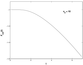
Figure 1: Using the ”square” dispersion relation (21): Nondimensional free energy $F_{red}(t)$ as defined by equation (38), versus nondimensional temperature $t=2\pi a/\beta$ when $x_{0}=10$.

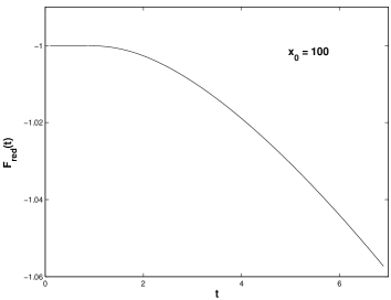
Figure 2: Same as figure 1, but with $x_{0}=100$.

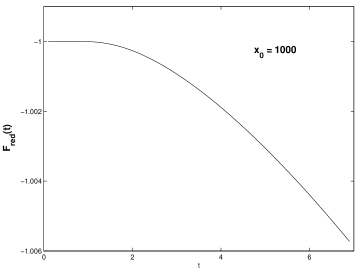
Figure 3: Same as figure 1, but with $x_{0}=1000$.

Figures 1 - 3 show how the nondimensional reduced Casimir free energy $F_{red}(t)$, defined by

$$F_{red}(t)\equiv\frac{F(T)}{3\xi^{2}x_{0}/(64a)},$$ (38)

varies with $t$, in the cases when $x_{0}=\{10,~{}100,~{}1000\}$. The low-temperature plateaus evidently lie at $F_{red}(0)=-1$. These figures are given on a linear scale, thus exhibiting the linear behaviour predicted by Eq. (37) at high temperatures. It is of interest to check the accuracy of (37) in cases when the condition (36) is reasonably well, but not extremely well, satisfied. Let us choose $x_{0}=10,~{}t=100$ as an example. From the expression

$$F_{red}(t\gg x_{0})=-\frac{8t}{3\pi x_{0}}\sum_{l=1}^{x_{0}}\frac{1}{\nu}$$ (39)

we obtain, taking into account that $\sum_{1}^{10}1/{\nu}=2.361749$, that $F_{red}(x_{0}=10,t=100)=-20.047149.$ The full series solution yields the number -20.047154. The approximate formula (39) is thus in this case extremely accurate. Choosing $t=10$, we get from Eq. (39) that $F_{red}(x_{0}=10,t=10)=-2.005$, whereas the series (31) yields -2.091. Even in this case, where the condition (36) obviously is broken, the error in the formula (39) is thus only about 4 per cent. Generally speaking, at high temperatures when the diluteness of the medium becomes more pronounced, the Casimir free energy becomes small, as we would expect.

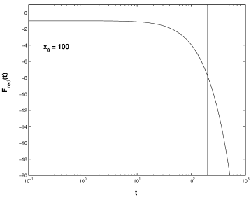
Figure 4: Same as figure 2, but with a logarithmic temperature scale. Vertical line represents $t=2x_{0}$.

In connection with the temperature dependence of the free energy the following physical argument should be noticed. From the dispersion relations (21) or (34) we would expect that the influence from the dispersion effect becomes important when the temperature becomes so high that the most significant frequencies in the thermal radiation field are of the same order as $\omega_{0}$. And as most significant thermal frequency, it is natural to take the value $\omega=\omega_{m}$ corresponding to the maximum of the blackbody distribution. From Wien’s dispacement law we know that $\omega_{m}=2.8/\beta$. Thus, we expect that dispersion becomes significant when $\omega\sim\omega_{0}\sim 2.8/\beta$ which, in view of the definition $t=2\pi a/\beta$, means that $t\sim 2x_{0}$. Now, in Figs. 1-3 the linear scale chosen for the temperature implies that the intervals covered on the ordinate axes are small, and the mentioned effect becomes hidden (the ”shoulder” in each diagram appears to lie at a lower value of $t$). The effect becomes however clear if we replace the linear temperature scale by a logarithmic scale. Figure 4 shows, as an example, such a diagram for the case $x_{0}=100$. Then the ordinate interval becomes considerably larger, and we see that the prediction $t\sim 2x_{0}$ for the position of the ”shoulder turns out to be reasonable. (In the diagram we have drawn the line $t=2x_{0}$ to emphasize the transitional region.) The same behaviour was previously found to hold in [8].

We note in passing that the high temperature entropy $S$ turns out to be constant: from Eq. (37) we get

$$S(t\gg x_{0})=-\frac{\partial F(T)}{\partial T}=\frac{\xi^{2}}{4}\sum_{l=1}^{x_{0}}\frac{1}{\nu}.$$ (40)

5 An improved dispersion relation

Instead of the formal divergence encountered in the previous section and the necessity to truncate the sum over $l$ in Eq. (28) at an upper limit $l=l_{0}$, it is of interest to consider a mathematically more involved but physically more correct dispersion relation, that leads to a finite result for the free energy even after summing over all $l$ up to infinity.

Let us consider the following dispersion relation, being essentially of the Lorentz form but augmented by a term in the denominator that describes spatial dispersion:

$$\mu(i\hat{\omega},l)-1=\frac{\chi_{0}}{1+(x^{2}+l^{2})/x_{0}^{2}},$$ (41)

$\chi_{0}$ being a constant. As in the previous section we assume that the ball of radius $a$ is dilute ($|\chi_{0}|\ll 1$), and that the exterior region is a vacuum. The spatial dispersion term $l^{2}/x_{0}^{2}$ ensures convergence when summing over all $l$. Since $\xi=(1-\mu)/(1+\mu)$ according to (7), we obtain to first order in $\chi_{0}$, at finite temperatures,

$$\xi\to\xi_{ln}=\frac{-\chi_{0}/2}{1+(n^{2}t^{2}+l^{2})/x_{0}^{2}}.$$ (42)

Instead of the expression (28) we now get

$$F(T)=-\frac{\xi_{0}^{2}x_{0}^{4}t}{8\pi a}\sum_{l=1}^{\infty}\left[\frac{1}{\nu(x_{0}^{2}+l^{2})^{2}}+\sum_{n=1}^{\infty}\frac{2\nu^{5}}{(x_{0}^{2}+l^{2}+n^{2}t^{2})^{2}(\nu^{2}+n^{2}t^{2})^{3}}\right],$$ (43)

where we have introduced the symbol $\xi_{0}=\chi_{0}/2$. We resolve the last term into partial fractions, and introduce the symbol $S(p;k)$:

$$S(p;k)=\sum_{n=1}^{\infty}(n^{2}+p^{2})^{-k}$$ (44)

Then, if $p$ and $q$ are arbitrary constants, we get

$$\sum_{n=1}^{\infty}\frac{1}{(n^{2}+p^{2})^{2}(n^{2}+q^{2})^{3}} = -\frac{3}{(p^{2}-q^{2})^{4}}S(p;1)-\frac{1}{(p^{2}-q^{2})^{3}}S(p;2)$$ (45)

$$+ \frac{3}{(p^{2}-q^{2})^{4}}S(q;1)-\frac{2}{(p^{2}-q^{2})^{3}}S(q;2)$$

$$+ \frac{1}{(p^{2}-q^{2})^{2}}S(q;3).$$

From Appendix A in [8] we write down the expressions for $S(p;k)$; $k=1,2$:

$$S(p;1)=-\frac{1}{2p^{2}}+\frac{\pi}{2p}\coth\pi p,$$ (46)

$$S(p;2)=-\frac{1}{2p^{4}}+\frac{\pi}{4p^{3}}\coth\pi p+\frac{\pi^{2}}{4p^{2}}\frac{1}{\sinh^{2}\pi p}$$ (47)

($S(p;3)$ was given in Eq. (30)). We define, in analogy with Eq. (38), the nondimensional reduced free energy to be

$$F_{red}(t)\equiv\frac{F(T)}{3\xi_{0}^{2}x_{0}/(64a)},$$ (48)

and obtain after some manipulations the following expression:

$$\begin{split}F_{red}(t)&=-\frac{16x_{0}^{3}t}{3\pi}\sum_{l=1}^{\infty}\left\{\frac{1}{2\nu(x_{0}^{2}+l^{2})^{2}}\right.\\ &-\frac{3\nu^{5}}{t^{2}(x_{0}^{2}-l-\frac{1}{4})^{4}}\left[S(\frac{\sqrt{x_{0}^{2}+l^{2}}}{t};1)\,-\;S(\frac{\nu}{t};1)\right]\\ &-\frac{\nu^{5}}{t^{4}(x_{0}^{2}-l-\frac{1}{4})^{3}}\left[S(\frac{\sqrt{x_{0}^{2}+l^{2}}}{t};2)+2S(\frac{\nu}{t};2)\right]\\ &+\left.\frac{\nu^{5}}{t^{6}(x_{0}^{2}-l-\frac{1}{4})^{2}}S(\frac{\nu}{t};3)\right\}.\end{split}$$ (49)

This expression is calculated numerically for two of the cases above, viz. $x_{0}=\{10,~{}100\}$. The results are shown in Fig. 5.

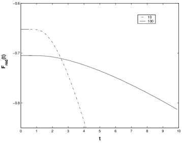
Figure 5: Using the spatial-dispersion relation (41): Nondimensional free energy $F_{red}(t)$ as defined by Eq. (48), versus nondimensional temperature $t=2\pi a/\beta$ when $x_{0}=\{10,~{}100\}$. The low-temperature plateau is in accordance with Eq. (54).

It is seen that the curves have roughly the same form as in Figs. 1 - 2. There is a definite low - temperature plateau, and for high values of $t$ the curves tend towards a linear form. In any case, whatever we adopt a square dispersion relation or a spatial - dispersion relation, the sensitivity with respect to increasing values of $t$ is most pronounced when $x_{0}$ is smallest. The limiting values for $t\rightarrow 0$ in Fig. 5 are in agreement with those of Figs. 1 and 2 to within about 70 per cent. This is the order of magnitude - agreement that we might expect, since the parameter $\xi_{0}$ made use of in Eq. (48) is similar to, but not identical with, the nondispersive quantity $\xi$ made use of in Eq. (38).

It is of interest to give analytic approximations for the case of low temperatures, $t\ll 1$. Then the quantities $p=\sqrt{x_{0}^{2}+l^{2}}/t$ and $q=\nu/t$ are large, and it becomes convenient to make use of the approximate formula [8, 34]

$$\sum_{n=1}^{\infty}\frac{1}{(n^{2}+p^{2})^{k}}=\frac{\sqrt{\pi}\Gamma(k-\frac{1}{2})}{2\Gamma(k)p^{2k-1}}-\frac{1}{2p^{2k}}+\left(\frac{\pi}{p}\right)^{k}\frac{e^{-2\pi p}}{\Gamma(k)},$$ (50)

from which it follows, in our notation, that

$$S(p;1)=\frac{\pi}{2p}-\frac{1}{2p^{2}}+\frac{\pi}{p}e^{-2\pi p},$$ (51)

$$S(p;2)=\frac{\pi}{4p^{3}}-\frac{1}{2p^{4}}+\left(\frac{\pi}{p}\right)^{2}e^{-2\pi p},$$ (52)

$$S(p;3)=\frac{3\pi}{16p^{5}}-\frac{1}{2p^{6}}+\frac{1}{2}\left(\frac{\pi}{p}\right)^{3}e^{-2\pi p}.$$ (53)

Inserting Eqs. (51)-(53) into Eq. (49) we obtain a reasonable simple series expression for $F_{red}(t)$, at low temperatures. A further simplification can be obtained if we keep only the leading order terms in Eqs. (51)-(53). For $p\gg 1$ this means that we keep only the first term in each equation. We then get in this limit

$$F_{red}(t\rightarrow 0) = x_{0}^{3}\sum_{l=1}^{\infty}\left\{\frac{8\nu^{5}}{(x_{0}^{2}-l-\frac{1}{4})^{4}}\left(\frac{1}{\sqrt{x_{0}^{2}+l^{2}}}-\frac{1}{\nu}\right)\right.$$ (54)

$$+ \left.\frac{8\nu^{5}}{3(x_{0}^{2}-l-\frac{1}{4})^{3}}\left(\frac{1}{2(x_{0}^{2}+l^{2})^{3/2}}+\frac{1}{\nu^{3}}\right)-\frac{1}{(x_{0}^{2}-l-\frac{1}{4})^{2}}\right\}.$$

In this expression, the temperature $t$ is no longer present. Numerical trials show that Eq. (54) is very accurate for $t\ll 1$. Choosing $x_{0}=10,~{}t=1$, we obtain from Eq. (54) $F_{red}(x_{0}=10,~{}t=1)=-0.6526$, whereas the full formula (49) yields the number -0.6530, i. e., an error of 0.06 per cent. Even with $t=2$, where Eq. (49) yields the number -0.678, the error in Eq. (54) is increased to only about 3 per cent.

6 Conclusion and final remarks

Let us summarize as follows:

(1) For a relativistic medium, i.e., a medium satisfying the condition $\epsilon\mu=1$, the $T=0$ result for the Casimir energy is most conveniently written in the form (8). This expression holds for a nondispersive medium, $\delta=\hat{\tau}/a$ being the time-splitting parameter. The permittivity is here arbitrary; the medium need not be dilute. The regularization is made by subtracting off the volume terms in the two scalar Green functions. This regularization is natural, among else things because it permits one to relate $E$ to the surface force density $f$ by the relation $\partial E/\partial a=-4\pi a^{2}f$. The equivalence between the Green function approach and the mode sum approach is demonstrated explicitly.

(2) As an additional by-result at $T=0$, the expression (15) generalizes the second order result for $E$ found in [15] up to the fourth order in the parameter $\xi$.

(3) Including the dispersive effect, the simplest dispersion relation one can imagine is the ”square” relation given in Eq. (21). The finite-temperature expression for the free energy on the basis of this dispersion relation is given in Eq. (31), with $x_{0}=\omega_{0}a$ being a high frequency cutoff which is in practice dependent on the detailed structure of the medium. With reasonable accuracy $x_{0}$ can represent the maximum $l_{0}$ of the angular momentum variable $l$. Typical results are shown in Figs. 1 - 4. In the limiting case $t\rightarrow 0$ they are in accordance with Eq. (33), and for $t\gg x_{0}$ they are in accordance with Eq. (39). In particular, the free energy is for high temperatures negative, and is a linear function of $t$. The entropy is correspondingly a (positive) constant. These results are in accordance with those of Refs. [26] and [27]. The transition region between low-temperature and high-temperature theory can be determined with reasonable accuracy from a simple physical argument.

These results are similar to those obtained on the basis of the Lorentz dispersion relation in [8].

(4) One can take spatial dispersion into account, as we have done in section 5. The basic dispersion relation is then Eq. (41). A physically appealing feature of this kind of approach is that the sum over angular momenta does not have to be truncated. Typical results for this case are shown in Fig. 5.

(5) The condition $\epsilon\mu=1$ simplifies the theory, as noted already in Ref. [4]. For an ordinary dielectric ball ($\mu=1$) the calculation becomes more complex and difficult to interpret [35].

(6) A final remark is called for, as regards the numerical computation of the series in the case of spatial dispersion. The evaluation of the expression (49) turned out to be more difficult than one might expect beforehand. Thus, a simple use of Matlab turned out to be insufficient. The problems seem to be associated with numerical noise, caused by the ”critical” terms for which $l\simeq x_{0}^{2}$. There are relatively large individual terms that almost, but not quite, compensate each other in the sum. We managed to do the calculation making use of double - precision MS-DOS Quick Basic. In practice, adequate precision was found with inclusion of less than $x_{0}^{2}$ terms.

Acknowledgment

We thank Michael Revzen and Israel Klich for valuable information about the finite temperature problem.

References

- [1] Plunien, G., Müller, B. and Greiner, W. 1986 Phys. Reports 134, 87.
- [2] Mostepanenko, V. M. and Trunov, N. N. 1997 The Casimir Effect and its Applications (London: Clarendon).
- [3] Milton, K. A. 1999 hep-th/9901011. Also in Applied Field Theory, Proc. 17th Symposium on Theoretical Physics, eds. C. Lee, H. Min and Q.-H. Park (Seoul: Chungburn, 1999).
- [4] Brevik, I. and Kolbenstvedt, H. 1982 Ann. Phys. NY 143, 179. Brevik, I. and Kolbenstvedt, H. 1983 Ann. Phys. NY 149, 237.
- [5] Brevik, I. and Kolbenstvedt, H. 1984 Can. J. Phys. 62, 805. Brevik, I. and Kolbenstvedt, H. 1985 Can. J. Phys. 63, 1409.
- [6] Milton, K. A., DeRaad, L. L., Jr. and Schwinger, J. 1978 Ann. Phys. NY 115, 388.
- [7] Brevik, I. and Einevoll, G. 1988 Phys. Rev. D 37, 2977.
- [8] Brevik, I. and Clausen, I. 1989 Phys. Rev. D 39, 603.
- [9] Brevik, I. 1987 J. Phys. A: Math. Gen. 20, 5189.
- [10] Brevik, I. and Sollie, R. 1990 J. Math. Phys. 31, 1445.
- [11] Brevik, I. and Nyland, G. H. 1994 Ann. Phys. NY 230, 321.
- [12] Milton, K. A. 1996 Proc. 3rd Workshop on Quantum Field Theory Under the Influence of External Conditions (Leipzig 1995), ed. M. Bordag (Stuttgart: Teubner) p. 13.
- [13] Milton, K. A. and Ng, Y. J. 1997 Phys. Rev. E 55, 4207.
- [14] Nesterenko, V. V. and Pirozhenko, I. G. 1997 Phys. Rev. D 57, 1284.
- [15] Brevik, I., Nesterenko, V. V. and Pirozhenko, I. G. 1998 J. Phys. A: Math. Gen. 31, 8661.
- [16] Lambiase, G., Nesterenko, V. V. and Bordag, M. 1999 J. Math. Phys. 40, 6254. Lambiase, G., Scarpetta, G. and Nesterenko, V. V. 1999 hep-th/9912176.
- [17] Nesterenko, V. V. and Pirozhenko, I. G. 1999 Phys. Rev. D. 60, 125007.
- [18] Klich, I. 2000 Phys. Rev. D 61, 025004.
- [19] Klich, I. 2000 Casimir Energy for Spherical and Cylindrical Boundary Conditions, MSc Thesis (Haifa: Israel Institute of Technology).
- [20] Lifshitz, E. M. 1955 Zh. Eksp. Teor. Fiz. 29, 94 [Sov. Phys. - JETP (USA) 2, 73 (1956)].
- [21] Fierz, M. 1960 Helv. Phys. Acta 33, 855.
- [22] Sauer, F. 1962 Ph.D. thesis (University of Göttingen).
- [23] Mehra, J. 1967 Physica 37, 145.
- [24] Brown, L. S. and Maclay, G. J. 1969 Phys. Rev. 184, 1272.
- [25] Milton, K. A., DeRaad, L. L., Jr. and Schwinger, J. 1978 Ann. Phys. NY 115, 1.
- [26] Revzen, M., Opher, R., Opher, M. and Mann, A. 1997 J. Phys. A: Math. Gen. 30, 7783.
- [27] Feinberg, J., Mann, A. and Revzen, M. 1999 hep-th/9908149.
- [28] Candelas, P. 1982 Ann. Phys. NY 143, 241.
- [29] Milton, K. A. 1980 Ann. Phys. NY 127, 49.
- [30] Brevik, I., Jensen, B. and Milton, K. A. 2000 hep-th/0004041.
- [31] Lambiase, G. and Nesterenko, V. V. 1996 Phys. Rev. D 54, 6387.
- [32] Nesterenko, V. V. and Pirozhenko, I. G. 1997 J. Math. Phys. 38, 6265.
- [33] Landau, L. D. and Lifshitz, E. M. 1984 Electrodynamics of Continuous Media, 2nd ed. (Oxford: Pergamon) p. 280.
- [34] Elizalde, E. 1995 Ten Physical Applications of Spectral Zeta Functions (Berlin: Springer).
- [35] Brevik, I. and Marachevsky, V. N. 1999 Phys. Rev. D 60, 085006.